2.29 numerical fluid mechanics lecture 17 slides · computational fluid dynamics for engineers....
TRANSCRIPT

2.29 Numerical Fluid Mechanics
Spring 2015 – L
2.29 Numerical Fluid Mechanics PFJL Lecture 17, 1
ecture 17
REVIEW Lecture 16: Finite Volume Methods
– Review: Basic elements of a FV scheme and steps to step-up a FV scheme
– One Dimensional examples
• Generic equation:
• Linear Convection (Sommerfeld eqn): convective fluxes
– 2nd order in space, then 4th order in space, links to CDS
• Unsteady Diffusion equation: diffusive fluxes
– Two approaches for 2nd order in space, links to CDS
– Two approaches for the approximation of surface integrals (and volume integrals)
– Interpolations and differentiations (express symbolic values at surfaces as a function of nodal variables)
• Upwind interpolation (UDS): (first-order and diffusive)
• Linear Interpolation (CDS): (2nd order, can be oscillatory)
• Quadratic Upwind interpolation (QUICK), convective flux
• Higher order (interpolation) schemes
if . 0
if . 0P e
eE e
v n
v n
(express symbolic values at surfaces as a function of nodal variables)
if . 0 if . 0 if . 0 v n if . 0 if . 0 if . 0UDS):
UDS):
UDS): UDS): UDS):
if . 0 if . 0
if . 0UDS): if . 0UDS): if . 0 UDS): UDS): if . 0UDS): UDS): e
UDS): e
UDS): if . 0 v n if . 0
if . 0 v n if . 0 UDS): UDS): if . 0UDS): UDS): v nUDS): UDS): if . 0UDS): UDS): if . 0 if . 0
if . 0 if . 0UDS): if . 0UDS): UDS): if . 0UDS):
(1 ) where e Pe E e P e e
E P
x xx x
1 2( ) ( )e U D U U UUg g
3 3
33
6 3 1 38 8 8 48e U D UU
D
x Rx
1/ 2
1/ 21/ 2 1/ 2 ( , )j
j
xjj j x
d xf f s x t dx
dt
E P
e E Px x x
PFJL Lecture 17, 2Numerical Fluid Mechanics2.29
TODAY (Lecture 17):
Numerical Methods for the Navier-Stokes Equations
• Solution of the Navier-Stokes Equations– Discretization of the convective and viscous terms– Discretization of the pressure term– Conservation principles– Choice of Variable Arrangement on the Grid– Calculation of the Pressure– Pressure Correction Methods
• A Simple Explicit Scheme• A Simple Implicit Scheme
– Nonlinear solvers, Linearized solvers and ADI solvers
• Implicit Pressure Correction Schemes for steady problems– Outer and Inner iterations
• Projection Methods– Non-Incremental and Incremental Schemes
• Fractional Step Methods: – Example using Crank-Nicholson

PFJL Lecture 17, 3Numerical Fluid Mechanics2.29
References and Reading Assignments
• Chapter 7 on “Incompressible Navier-Stokes equations” of “J. H. Ferziger and M. Peric, Computational Methods for Fluid Dynamics. Springer, NY, 3rd edition, 2002”
• Chapter 11 on “Incompressible Navier-Stokes Equations” of T. Cebeci, J. P. Shao, F. Kafyeke and E. Laurendeau, Computational Fluid Dynamics for Engineers. Springer, 2005.
• Chapter 17 on “Incompressible Viscous Flows” of Fletcher, Computational Techniques for Fluid Dynamics. Springer, 2003.

PFJL Lecture 17, 4Numerical Fluid Mechanics2.29
= Symmetric formula for e: no need for “upwind” as with 0th or 2nd order polynomials (donor-cell & QUICK)
– With (x), one can insert e= (xe) in symbolic integral formula. For a uniform Cartesian grid:
• Convective Fluxes: (similar formulas used for ϕ values at corners)
• For Diffusive Fluxes (1st derivative):
– This FV approximation often called a 4th-order CDS (linear poly. interpol. was 2nd-order CDS)
– Polynomials of higher-degree or of multi-dimensions can be used, as well as cubic splines (to ensure continuity of first two derivatives at the boundaries). This increases the cost.
Interpolations and Differentiations(to obtain fluxes “Fe= f (e)” as a function of cell-average values)
• Higher Order Schemes (for convective/diffusive fluxes)
– Interpolations of order of accuracy higher than 3 make sense if
yj+1
xi-1 xi xi+1
yj-1
y
ji
x
yj
NW
WW W
SW S SE
E EE
N NE
∆y
∆x
nw
s
nw neneP
sw se
e
yj+1
xi-1 xi xi+1
yj-1
y
ji
x
yj
NW
WW W
SW S SE
E EE
N NE
∆y
∆x
nw
s
nw neneP
sw se
eintegrals are also approximated with higher order formulas
– In 1D problems, if Simpson’s rule (4th order error) is used for the integral, a polynomial interpolation of order 3 can be used:
=> 4 unknowns, hence 4 nodal values (W, P, E and EE) needed
2 30 1 2 3( )x a a x a x a x
21 2 3
27 272 3 for a uniform Cartesian grid: 24
E P W EE
e e
a a x a xx x x
27 27 3 348
P E W EEe
( Note: higher-order, approach 1 →≈ approach 2 ! )
Notation used for a Cartesian 2D and 3D grid.Image by MIT OpenCourseWare.

PFJL Lecture 17, 5Numerical Fluid Mechanics2.29
– Ex. 2: use a parabola, fit the values on either side of the cell face and the derivative on the upstream side (equivalent to the QUICK scheme, 3rd order)
– Similar schemes are obtained for derivatives (diffusive fluxes), see Ferziger and Peric (2002)
• Other Schemes: more complex and difficult to program
– Large number of approximations used for “convective” fluxes: Linear Upwind Scheme, Skewed Upwind schemes, Hybrid. Blending schemes to eliminate oscillations at higher order.
Interpolations and Differentiations(to obtain fluxes “Fe= f (e)” as a function of cell-average values)
• Compact Higher Order Schemes
– Polynomial of higher order lead too large computational
molecules => use deferred-correction schemes and/or
compact (Pade’) schemes
– Ex. 1: obtain the coefficients of by
yj+1
xi-1 xi xi+1
yj-1
y
ji
x
yj
NW
WW W
SW S SE
E EE
N NE
∆y
∆x
nw
s
nw neneP
sw se
e
yj+1
xi-1 xi xi+1
yj-1
y
ji
x
yj
NW
WW W
SW S SE
E EE
N NE
∆y
∆x
nw
s
nw neneP
sw se
e
fitting two values and two 1st derivatives at the two nodes on
either side of the cell face. With evaluation at xe:
• 4th order scheme:
• If we use CDS to approximate derivatives, result retains 4th order:
2 30 1 2 3( )x a a x a x a x
3 1 x+ 4 4 4e U D
Ux
4( )2 8
P Ee
P E
x O xx x
4( )2 16
P E P E W EEe O x
Notation used for a Cartesian 2D and 3D grid.Image by MIT OpenCourseWare.
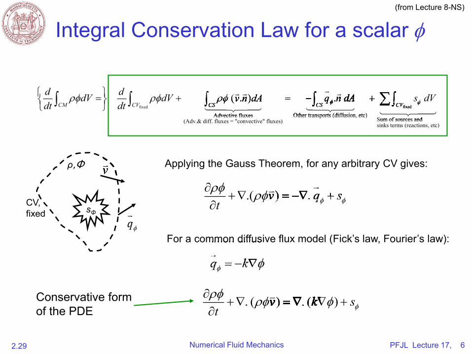
Integral Conservation Law for a scalar
2.29 Numerical Fluid Mechanics PFJL Lecture 17, 6
fixed fixed
Advective fluxes Other transports (diffusion, etc)Sum of sources and(Adv.& diff. fluxes = "convective" fluxes)sinks
( . ) .CM CV CS CS CV
d ddV dV v n dA q n dA s dVdt dt
v n dA( . )v n dA( . ) q n dA q n dA q n dA q n dA
Advective fluxes Other transports (diffusion, etc)
( . )CS CS
v n dA( . )v n dA( . ) CS CS CS CSq n dA q n dA q n dA q n dA q n dA q n dA.q n dA. .q n dA. .q n dA. .q n dA. v n dA( . )v n dA( . ) q n dA q n dA q n dA q n dA q n dA q n dA.q n dA. .q n dA. .q n dA. .q n dA.
terms (reactions, etc)
fixed
Sum of sources and
CVfixedCVfixed CV CV
. ( ) . ( )v k st
. ( ) . ( )v k s. ( ) . ( ) . ( ) . ( )v k s. ( ) . ( ). ( ) . ( )v k s. ( ) . ( ) . ( ) . ( )v k s. ( ) . ( ) . ( ) . ( )v k s. ( ) . ( ) . ( ) . ( )v k s. ( ) . ( )
CV,fixed sΦ
ρ,Φ vv
.( ) .v q st
v q s v q s v q s.( ) ..( ) ..( ) . .( ) . .( ) .v q s v q s.( ) .v q s.( ) . .( ) .v q s.( ) ..( ) ..( ) . .( ) ..( ) ..( ) .v q s.( ) ..( ) .v q s.( ) . .( ) .v q s.( ) ..( ) .v q s.( ) . v q s v q s
Applying the Gauss Theorem, for any arbitrary CV gives:
For a common diffusive flux model (Fick’s law, Fourier’s law):
q k
ommon diffusffusf
q k q k q k
Conservative form of the PDE
(from Lecture 8-NS)

Strong-Conservative form
of the Navier-Stokes Equations ( v)
2.29 Numerical Fluid Mechanics PFJL Lecture 17, 7
CV,fixed sΦ
ρ,Φ vv.( ) .v v v p g
t
.( ) .v .( ) .v v p gv v p g v v p g .( ) . .( ) .v v p g v v p g.( ) .v v p g.( ) . .( ) .v v p g.( ) . v v p g v v p g v v p g v v p g.( ) .v v p g.( ) . .( ) .v v p g.( ) . .( ) .v v p g.( ) . .( ) .v v p g.( ) ..( ) .v v p g v v p g v v p g v v p g v v p g v v p g v v p g.( ) .v v p g.( ) . .( ) .v v p g.( ) ..( ) ..( ) . .( ) ..( ) .v v p g.( ) . .( ) .v v p g.( ) .
Applying the Gauss Theorem gives:
Equations are said to be in “strong conservative form” if all terms have the form of the divergence of a vector or a tensor. For the i th Cartesian component, in the general Newtonian fluid case:
( . ) .
.
CV CS CS CS CV
F
CV
d vdV v v n dA p ndA ndA gdVdt
p g dV
F
vdV v v n dA p ndA ndA gdVvdV v v n dA p ndA ndA gdV vdV v v n dA p ndA ndA gdV vdV v v n dA p ndA ndA gdV vdV v v n dA p ndA ndA gdV( . )vdV v v n dA p ndA ndA gdV( . ) ( . )vdV v v n dA p ndA ndA gdV( . )vdV v v n dA p ndA ndA gdV vdV v v n dA p ndA ndA gdV vdV v v n dA p ndA ndA gdV vdV v v n dA p ndA ndA gdVvdV v v n dA p ndA ndA gdV vdV v v n dA p ndA ndA gdV vdV v v n dA p ndA ndA gdV vdV v v n dA p ndA ndA gdVvdV v v n dA p ndA ndA gdVvdV v v n dA p ndA ndA gdV vdV v v n dA p ndA ndA gdVvdV v v n dA p ndA ndA gdVvdV v v n dA p ndA ndA gdV vdV v v n dA p ndA ndA gdVvdV v v n dA p ndA ndA gdV vdV v v n dA p ndA ndA gdV vdV v v n dA p ndA ndA gdV vdV v v n dA p ndA ndA gdVvdV v v n dA p ndA ndA gdV vdV v v n dA p ndA ndA gdVvdV v v n dA p ndA ndA gdV vdV v v n dA p ndA ndA gdV vdV v v n dA p ndA ndA gdV vdV v v n dA p ndA ndA gdVvdV v v n dA p ndA ndA gdV vdV v v n dA p ndA ndA gdV vdV v v n dA p ndA ndA gdV vdV v v n dA p ndA ndA gdV vdV v v n dA p ndA ndA gdV vdV v v n dA p ndA ndA gdV vdV v v n dA p ndA ndA gdV vdV v v n dA p ndA ndA gdVvdV v v n dA p ndA ndA gdVvdV v v n dA p ndA ndA gdV vdV v v n dA p ndA ndA gdV vdV v v n dA p ndA ndA gdV vdV v v n dA p ndA ndA gdVvdV v v n dA p ndA ndA gdV vdV v v n dA p ndA ndA gdV vdV v v n dA p ndA ndA gdV vdV v v n dA p ndA ndA gdVvdV v v n dA p ndA ndA gdV vdV v v n dA p ndA ndA gdV vdV v v n dA p ndA ndA gdV vdV v v n dA p ndA ndA gdVvdV v v n dA p ndA ndA gdV vdV v v n dA p ndA ndA gdV vdV v v n dA p ndA ndA gdV vdV v v n dA p ndA ndA gdV vdV v v n dA p ndA ndA gdV vdV v v n dA p ndA ndA gdV vdV v v n dA p ndA ndA gdV vdV v v n dA p ndA ndA gdVCS CS CV
F
vdV v v n dA p ndA ndA gdVvdV v v n dA p ndA ndA gdV vdV v v n dA p ndA ndA gdVCV
vdV v v n dA p ndA ndA gdVCV
CV
vdV v v n dA p ndA ndA gdVCV
CS CS CS CS CV CVvdV v v n dA p ndA ndA gdV vdV v v n dA p ndA ndA gdV
CSvdV v v n dA p ndA ndA gdV
CS CSvdV v v n dA p ndA ndA gdV
CS CSvdV v v n dA p ndA ndA gdV
CS CSvdV v v n dA p ndA ndA gdV
CSvdV v v n dA p ndA ndA gdV vdV v v n dA p ndA ndA gdV vdV v v n dA p ndA ndA gdV vdV v v n dA p ndA ndA gdV.vdV v v n dA p ndA ndA gdV. .vdV v v n dA p ndA ndA gdV. .vdV v v n dA p ndA ndA gdV. .vdV v v n dA p ndA ndA gdV.
CVvdV v v n dA p ndA ndA gdV
CV
CVvdV v v n dA p ndA ndA gdV
CV CVvdV v v n dA p ndA ndA gdV
CV
CVvdV v v n dA p ndA ndA gdV
CVvdV v v n dA p ndA ndA gdV vdV v v n dA p ndA ndA gdV vdV v v n dA p ndA ndA gdV vdV v v n dA p ndA ndA gdVvdV v v n dA p ndA ndA gdV vdV v v n dA p ndA ndA gdV vdV v v n dA p ndA ndA gdV vdV v v n dA p ndA ndA gdV vdV v v n dA p ndA ndA gdV vdV v v n dA p ndA ndA gdV vdV v v n dA p ndA ndA gdV vdV v v n dA p ndA ndA gdV.vdV v v n dA p ndA ndA gdV. .vdV v v n dA p ndA ndA gdV. .vdV v v n dA p ndA ndA gdV. .vdV v v n dA p ndA ndA gdV. .vdV v v n dA p ndA ndA gdV. .vdV v v n dA p ndA ndA gdV. .vdV v v n dA p ndA ndA gdV. .vdV v v n dA p ndA ndA gdV.
F
vdV v v n dA p ndA ndA gdVvdV v v n dA p ndA ndA gdV vdV v v n dA p ndA ndA gdVvdV v v n dA p ndA ndA gdV vdV v v n dA p ndA ndA gdV vdV v v n dA p ndA ndA gdV vdV v v n dA p ndA ndA gdVvdV v v n dA p ndA ndA gdV vdV v v n dA p ndA ndA gdV vdV v v n dA p ndA ndA gdV vdV v v n dA p ndA ndA gdVvdV v v n dA p ndA ndA gdV vdV v v n dA p ndA ndA gdV vdV v v n dA p ndA ndA gdV vdV v v n dA p ndA ndA gdV vdV v v n dA p ndA ndA gdV vdV v v n dA p ndA ndA gdV vdV v v n dA p ndA ndA gdV vdV v v n dA p ndA ndA gdV.vdV v v n dA p ndA ndA gdV. .vdV v v n dA p ndA ndA gdV. .vdV v v n dA p ndA ndA gdV. .vdV v v n dA p ndA ndA gdV. .vdV v v n dA p ndA ndA gdV. .vdV v v n dA p ndA ndA gdV. .vdV v v n dA p ndA ndA gdV. .vdV v v n dA p ndA ndA gdV.
F
p g dVp g dVp g dV p g dVp g dV p g dV p g dV p g dVp g dVp g dVp g dV p g dV
p g dV p g dVp g dV p g dV p g dV p g dV
With Newtonian fluid + incompressible + constant μ:
For any arbitrary CV gives:
2.( )
. 0
v v v p v gtv
.( )v 2.( )v v p v g v v p v g v v p v g 2 2.( ) .( )v v p v g v v p v g.( )v v p v g.( ) .( )v v p v g.( ) 2 2 2 2v v p v g v v p v g v v p v g v v p v g.( )v v p v g v v p v g.( )v v p v g.( ) .( )v v p v g.( ).( ) .( ) .( )v v p v g v v p v g.( )v v p v g.( ) .( )v v p v g.( )
. 0t
. 0 . 0. 0v. 0 . 0v. 0
Momentum:
Mass:
2.( ) .3
j ji ii i j i i i i
j i j
u uv uv v p e e e g x et x x x
u u u u v u v u v u v u 2 2 2 2u u u u u u u u2u u2 2u u2 2u u2 2u u2 u u u u u u u u u u u u u u u u v u v u v u v u v u v u v u v u v u v u v u v u
j j
j j2j j2
2j j2j ju uj j
j ju uj je e g x e e e g x e e e g x e e e g x e e e g x e e e g x e
j j
j j
j j
j ju u u u
u u u uj ju uj j
j ju uj j
j ju uj j
j ju uj j
v u v u
v u v u v u v u v u v u
v u v u v u v u j j j j
j j j j2j j2 2j j2
2j j2 2j j2j ju uj j j ju uj j
j ju uj j j ju uj j2j j2u u2j j2 2j j2u u2j j2
2j j2u u2j j2 2j j2u u2j j2u u u u u u u u
u u u u u u u u2u u2 2u u2 2u u2 2u u2
2u u2 2u u2 2u u2 2u u2j ju uj j
j ju uj j j ju uj j
j ju uj j
j ju uj j
j ju uj j j ju uj j
j ju uj j2j j2u u2j j2 2j j2u u2j j2 2j j2u u2j j2 2j j2u u2j j2
2j j2u u2j j2 2j j2u u2j j2 2j j2u u2j j2 2j j2u u2j j2
u u u u u u u u
u u u u u u u uj ju uj j j ju uj j j ju uj j j ju uj j
j ju uj j j ju uj j j ju uj j j ju uj j u u u u u u u u u u u u u u u u
u u u u u u u u u u u u u u u uj ju uj j
j ju uj j j ju uj j
j ju uj j j ju uj j
j ju uj j j ju uj j
j ju uj j
j ju uj j
j ju uj j j ju uj j
j ju uj j j ju uj j
j ju uj j j ju uj j
j ju uj jv u v u
v u v ui iv ui i i iv ui i i iv ui i i iv ui iv u v u v u v u
v u v u v u v uv u v u v u v u
v u v u v u v uv u v u v u v u v u v u v u v u
v u v u v u v u v u v u v u v u
j j
j j
j j
j j2j j2
2j j2
2j j2
2j j2i i i i i i i iv v p e v v p e v v p e v v p ei iv v p ei i i iv v p ei i i iv v p ei i i iv v p ei i e e g x e e e g x e e e g x e e e g x ej je e g x ej j
j je e g x ej j
j je e g x ej j
j je e g x ej j i ii i i ii i i ii i i ii i j j j j
j j j j
j j j j
j j j je e g x e e e g x e e e g x e e e g x e e e g x e e e g x e e e g x e e e g x ej je e g x ej j j je e g x ej j
j je e g x ej j j je e g x ej j
j je e g x ej j j je e g x ej j
j je e g x ej j j je e g x ej ji i i i i i i i i i i i i i i ii iv ui i i iv ui i i iv ui i i iv ui i i iv ui i i iv ui i i iv ui i i iv ui i j j
j j
j j
j ji i i i
i i i ii iv ui i i iv ui i
i iv ui i i iv ui i
j j j j
j j j j
j j j j
j j j ji i
i i i i
i i
i i
i i i i
i iv u v u
v u v u
v u v u
v u v ui iv ui i
i iv ui i i iv ui i
i iv ui i
i iv ui i
i iv ui i i iv ui i
i iv ui i
j j j j j j j j
j j j j j j j j
j j j j j j j j
j j j j j j j ju u u u u u u u
u u u u u u u u
u u u u u u u u
u u u u u u u uj ju uj j j ju uj j j ju uj j j ju uj j
j ju uj j j ju uj j j ju uj j j ju uj j
j ju uj j j ju uj j j ju uj j j ju uj j
j ju uj j j ju uj j j ju uj j j ju uj ji iv ui i i iv ui i i iv ui i i iv ui i
i iv ui i i iv ui i i iv ui i i iv ui iv u v u v u v u
v u v u v u v u
v u v u v u v u
v u v u v u v ui iv ui i
i iv ui i i iv ui i
i iv ui i i iv ui i
i iv ui i i iv ui i
i iv ui i
i iv ui i
i iv ui i i iv ui i
i iv ui i i iv ui i
i iv ui i i iv ui i
i iv ui i
j j
j j
j j
j j
j j
j j
j j
j ji i i i i i i i
i i i i i i i ii iv ui i i iv ui i i iv ui i i iv ui i
i iv ui i i iv ui i i iv ui i i iv ui ii i i i i i i i i i i i i i i i
i i i i i i i i i i i i i i i ii iv ui i i iv ui i i iv ui i i iv ui i i iv ui i i iv ui i i iv ui i i iv ui i
i iv ui i i iv ui i i iv ui i i iv ui i i iv ui i i iv ui i i iv ui i i iv ui i
j j
j j
j j
j j
j j
j j
j j
j j
j j
j j
j j
j j
j j
j j
j j
j ji i i i i i i i
i i i i i i i i
i i i i i i i i
i i i i i i i i
i i i i i i i i i i i i i i i ie e g x e e e g x e
e e g x e e e g x ei i i ie e g x ei i i i i i i ie e g x ei i i i i i i ie e g x ei i i i i i i ie e g x ei i i ie e g x e e e g x e e e g x e e e g x e
e e g x e e e g x e e e g x e e e g x ei i i ie e g x ei i i i i i i ie e g x ei i i i i i i ie e g x ei i i i i i i ie e g x ei i i i i i i ie e g x ei i i i i i i ie e g x ei i i i i i i ie e g x ei i i i i i i ie e g x ei i i i
e e g x e e e g x e e e g x e e e g x e
e e g x e e e g x e e e g x e e e g x ee e g x e e e g x e e e g x e e e g x e
e e g x e e e g x e e e g x e e e g x eje e g x ej je e g x ej je e g x ej je e g x ej je e g x ej je e g x ej je e g x ej je e g x eje e g x e e e g x e e e g x e e e g x e e e g x e e e g x e e e g x e e e g x e
e e g x e e e g x e e e g x e e e g x e e e g x e e e g x e e e g x e e e g x ee e g x e e e g x e e e g x e e e g x e e e g x e e e g x e e e g x e e e g x e
e e g x e e e g x e e e g x e e e g x e e e g x e e e g x e e e g x e e e g x ei i i ie e g x ei i i i i i i ie e g x ei i i i i i i ie e g x ei i i i i i i ie e g x ei i i i i i i ie e g x ei i i i i i i ie e g x ei i i i i i i ie e g x ei i i i i i i ie e g x ei i i i i i i ie e g x ei i i i i i i ie e g x ei i i i i i i ie e g x ei i i i i i i ie e g x ei i i i i i i ie e g x ei i i i i i i ie e g x ei i i i i i i ie e g x ei i i i i i i ie e g x ei i i i
i i i i i i i iv v p e v v p e v v p e v v p e
v v p e v v p e v v p e v v p eiv v p ei iv v p ei iv v p ei iv v p ei iv v p ei iv v p ei iv v p ei iv v p ei
v u v ui iv ui i i iv ui i.( ) .i i.( ) .v u.( ) .i i.( ) . .( ) .i i.( ) .v u.( ) .i i.( ) . v u v u v u v ui i i i.( ) .i i.( ) . .( ) .i i.( ) .v v p e v v p e.( ) .v v p e.( ) . .( ) .v v p e.( ) .i iv v p ei i i iv v p ei i.( ) .i i.( ) .v v p e.( ) .i i.( ) . .( ) .i i.( ) .v v p e.( ) .i i.( ) .i i i i i i i i.( ) .i i.( ) . .( ) .i i.( ) . .( ) .i i.( ) . .( ) .i i.( ) .i iv ui i i iv ui i i iv ui i i iv ui i.( ) .i i.( ) .v u.( ) .i i.( ) . .( ) .i i.( ) .v u.( ) .i i.( ) . .( ) .i i.( ) .v u.( ) .i i.( ) . .( ) .i i.( ) .v u.( ) .i i.( ) .v u v u
v u v ui iv ui i i iv ui i i iv ui i i iv ui iv u v u v u v u
v u v u v u v ui i i i i i i iv v p e v v p e v v p e v v p ei iv v p ei i i iv v p ei i i iv v p ei i i iv v p ei ii i i i i i i i i i i i i i i ii iv ui i i iv ui i i iv ui i i iv ui i i iv ui i i iv ui i i iv ui i i iv ui iv v p e v v p e v v p e v v p e
v v p e v v p e v v p e v v p eWith Newtonian fluid only:
Cons. of Momentum:
Cauchy Mom. Eqn.
(from Lecture 8-NS)

Solution of the Navier-Stokes Equations
• In the FD and FV schemes, we dealt with the discretization of the generic conservation equation
• These results apply to the momentum and continuity equations (the NS equations), e.g. for incompressible flows, constant viscosity
• Terms that are discretized similarly
– Unsteady and advection terms: they have the same form for scalar than for ⇒ v
• Terms that are discretized differently
– Momentum (vector) diffusive fluxes need to be treated in a bit more details
– Pressure term has no analog in the generic conservation equation => needs special attention. It can be regarded either as a
• source term (treated non-conservatively as a body force), or as,
• surface force (conservative treatment)
– Finally, main variable v is a vector gives more freedom to the choice of grids
2.29 Numerical Fluid Mechanics PFJL Lecture 17, 8
.( ) .v q st
v q s v q s v q s.( ) ..( ) ..( ) . .( ) . .( ) .v q s v q s.( ) .v q s.( ) . .( ) .v q s.( ) ..( ) ..( ) . .( ) ..( ) ..( ) .v q s.( ) ..( ) .v q s.( ) . .( ) .v q s.( ) ..( ) .v q s.( ) . v q s v q s
2.( )
. 0
v v v p v gtv
equations), e.g. for incompressible flows, constant viscosity
.( )vflows, constant viscosity
2.( )v v p v g v v p v g v v p v g 2 2v v p v g v v p v g.( ) .( ).( )v v p v g.( ) .( )v v p v g.( ) 2 2 2 2v v p v g v v p v g v v p v g v v p v g
flows, constant viscosity
.( )v v p v g v v p v g.( )v v p v g.( ) .( )v v p v g.( )
flows, constant viscosity
.( ) .( ) .( )v v p v g v v p v g.( )v v p v g.( ) .( )v v p v g.( )
. 0t
. 0 . 0. 0v. 0 . 0v. 0

Discretization of the
Convective and Viscous Terms
• Convective term:
– Use any of the schemes (FD or FV) that we have seen (including complex geometries)
• Viscous term:
– For a Newtonian Fluid and incompressible flows:
• If μ is constant, the viscous term is as in the general conservation eqn. for
• If μ varies, its derivative needs to be evaluated (FD scheme) or its variations accounted for in the integrals (for a FV scheme)
– For a Newtonian fluid and compressible flow:
• Additional terms need to be treated, e.g.
– Note that in non-Cartesian coordinate systems, new terms also arise that behave as a “body force”, and can thus be treated explicitly or implicitly
• e.g2.29 Numerical Fluid Mechanics PFJL Lecture 17, 9
( ).( ) and ( . ) and ( . )i j
iS Sj
u uv v v v n dS u v n dS
x
Convective term: Convective term: v v v v n dSConvective term: Convective term: .( ) and ( . )Convective term: v v v v n dSConvective term: .( ) and ( . )Convective term:
( ) ( )( )u u( ) ( )u u( )( )( ) ( )( ) and ( . ) and ( . )u v n dS u v n dS and ( . )u v n dS and ( . ) and ( . )u v n dS and ( . ) and ( . ) and ( . ) and ( . ) and ( . ) and ( . ) and ( . )
and ( . ) and ( . )u v n dS u v n dS
u v n dS u v n dS and ( . )u v n dS and ( . ) and ( . )u v n dS and ( . )
and ( . )u v n dS and ( . ) and ( . )u v n dS and ( . ) and ( . )i and ( . )u v n dS and ( . )i and ( . ) and ( . )i and ( . )u v n dS and ( . )i and ( . )
and ( . )i and ( . )u v n dS and ( . )i and ( . ) and ( . )i and ( . )u v n dS and ( . )i and ( . ) and ( . ) and ( . ) and ( . ) and ( . )
and ( . ) and ( . ) and ( . ) and ( . ) Convective term: Convective term: v v v v n dS v v v v n dSConvective term: v v v v n dSConvective term: Convective term: v v v v n dSConvective term: Convective term: .( ) and ( . )Convective term: v v v v n dSConvective term: .( ) and ( . )Convective term: Convective term: .( ) and ( . )Convective term: v v v v n dSConvective term: .( ) and ( . )Convective term: Convective term: .( ) and ( . )Convective term: v v v v n dSConvective term: .( ) and ( . )Convective term: Convective term: .( ) and ( . )Convective term: v v v v n dSConvective term: .( ) and ( . )Convective term: Convective term: .( ) and ( . )Convective term: v v v v n dSConvective term: .( ) and ( . )Convective term: Convective term: .( ) and ( . )Convective term: v v v v n dSConvective term: .( ) and ( . )Convective term:
( ) ( )
( ) ( )( )i j( ) ( )i j( )
( )i j( ) ( )i j( )( )u u( ) ( )u u( )
( )u u( ) ( )u u( )( )i j( )u u( )i j( ) ( )i j( )u u( )i j( )
( )i j( )u u( )i j( ) ( )i j( )u u( )i j( )( )( ) ( )( )
( )( ) ( )( )
( )
( )
( )
( ) and ( . ) and ( . ) and ( . ) and ( . )i j
i j
i j
i j( )i j( )
( )i j( )
( )i j( )
( )i j( )
( )( )
( )( )
( )( )
( )( )
( ) ( )
( ) ( )
( ) ( )
( ) ( )( )i j( ) ( )i j( )
( )i j( ) ( )i j( )
( )i j( ) ( )i j( )
( )i j( ) ( )i j( )( )u u( ) ( )u u( )
( )u u( ) ( )u u( )
( )u u( ) ( )u u( )
( )u u( ) ( )u u( )( )i j( )u u( )i j( ) ( )i j( )u u( )i j( )
( )i j( )u u( )i j( ) ( )i j( )u u( )i j( )
( )i j( )u u( )i j( ) ( )i j( )u u( )i j( )
( )i j( )u u( )i j( ) ( )i j( )u u( )i j( )( )( ) ( )( )
( )( ) ( )( )
( )( ) ( )( )
( )( ) ( )( )
and ( . ) and ( . )
and ( . ) and ( . ) and ( . ) and ( . )
and ( . ) and ( . )i j
i j
i j
i j
i j
i j
i j
i j.( ) and ( . )v v v v n dS.( ) and ( . )Convective term: .( ) and ( . )Convective term: v v v v n dSConvective term: .( ) and ( . )Convective term: .( ) and ( . )v v v v n dS.( ) and ( . ) .( ) and ( . )v v v v n dS.( ) and ( . )Convective term: .( ) and ( . )Convective term: v v v v n dSConvective term: .( ) and ( . )Convective term: Convective term: .( ) and ( . )Convective term: v v v v n dSConvective term: .( ) and ( . )Convective term: Convective term: Convective term: v v v v n dSConvective term: Convective term: .( ) and ( . )Convective term: v v v v n dSConvective term: .( ) and ( . )Convective term: Convective term: Convective term: Convective term: v v v v n dSConvective term: Convective term: v v v v n dSConvective term: Convective term: .( ) and ( . )Convective term: v v v v n dSConvective term: .( ) and ( . )Convective term: Convective term: .( ) and ( . )Convective term: v v v v n dSConvective term: .( ) and ( . )Convective term:
. and . and .ijij jS S
j
ndA e n dSx
and . and .e n dS e n dS and .e n dS and . and .e n dS and . and . and . and . and .
. and . . and . and . and .
and . and . and .ij j and . and .ij j and .
and .ij j and . and .ij j and .e n dS e n dS
e n dS e n dS and .e n dS and . and .e n dS and .
and .e n dS and . and .e n dS and . and .ij j and .e n dS and .ij j and . and .ij j and .e n dS and .ij j and .
and .ij j and .e n dS and .ij j and . and .ij j and .e n dS and .ij j and . and . and . and . and .
and . and . and . and .
ij ij
ij ij
and . and . and . and .ij
ij
ij
ij
ij ij
ij ij
ij ij
ij ij
. and . . and .ndA ndA. and . . and . . and . . and . and . and .
and . and . and . and .
and . and .ij
ij
ij
ij
ij
ij
ij
ij. and .. and . . and .
. and . . and .ndA ndA. and . . and . . and . . and .
jiij
j i
uux x
22 rur
23
ji
j
ue
x
ie

Discretization of the Pressure term
– For conservative NS schemes, gravity/body-force terms often included in the “pressure” term, giving:
• “Pressure” then part of the stress tensor (shows up as divergence in NS eqns.)
• Last term is null for incompressible flows
– In non-conservative NS forms, the pressure gradient is discretized
• FD schemes
– FD schemes seen earlier are directly applicable, but pressure can be discretized on a different grid than the velocity grid (staggered grid)
• FV schemes
– Pressure usually treated as a surface force (conservative form):
• For the u equation:i
• Again, schemes seen in previous lectures are applicable, but pressure nodes can be on a different CV grid
– Pressure can also be treated non-conservatively:
• Discretization then introduces a global non-conservative error
2.29 Numerical Fluid Mechanics PFJL Lecture 17, 10
2 2. . ( )3 3
ji i i i i
j
up p p e g x e e
x
g r u
terms often included in 2 2 )j
i
up e g x e ep e g x e ejp e g x e ej
ip e g x e ei p e g x e e p e g x e ep e g x e e p e g x e e
2 2
2 2p e g x e e p e g x e ei i i ip e g x e ei i i i i i i ip e g x e ei i i i p e g x e e p e g x e e p e g x e e p e g x e ei i i ip e g x e ei i i i i i i ip e g x e ei i i i i i i ip e g x e ei i i i i i i ip e g x e ei i i ip p p p p p g r u g r u g r u
.iSp e ndS
as a surface force (conservative form):
p e ndS.p e ndS.ip e ndSi
. iVp e dV p e dVip e dVi

PFJL Lecture 17, 11Numerical Fluid Mechanics2.29
Conservation Principles for NS
• Momentum and Mass Conservation
– Momentum is conserved in any control volume in the sense that “it can only change because of flow through the CV surfaces, forces acting on these surfaces or volumetric body forces”
– This property is inherited in the CV formulation (if surface fluxes are identical on both sides)
– Similar statements for Mass conservation
• Conservation of important secondary quantities, e.g. energy
– More complex issues
– In heat transfer, thermal energy equation can be solved after momentum equation has been solved if properties don’t vary much with temperature T T is then a passive scalar, with one way coupling
– In incompressible, isothermal flows: kinetic energy is the significant energy
– In compressible flows: energy includes compressible terms
total energy is then a separate equation (1st law) but a second derived equation can still be written, either for kinetic or internal energy

Conservation Principles for NS: Cont’dKinetic Energy Conservation
• Derivation of Kinetic energy equation
– Take dot product of momentum equation with velocity
– Integrate over a control volume CV or full volume of domain of interest
– This gives
where is the viscous component of the stress tensor
– In the volume integral of the RHS, the three terms are zero if the flow is inviscid
(term 1 = dissipation), incompressible (term 2) and there are no body forces (term 3)
– Other terms are surface terms and kinetic energy is conserved in this sense:
discretization on CV should ideally lead to no contribution over the volume
• Some observations
– Guaranteeing global conservation of the discrete kinetic energy is not automatic
since the kinetic energy equation is a consequence of the momentum equation.
– Discrete momentum and kinetic energy conservations cannot be enforced
separately (the latter can only be a consequence of the former)2.29 Numerical Fluid Mechanics PFJL Lecture 17, 12
2 2
( . ) . ( . ). : . .2 2CV CS CS CS CV
v vdV v n dA p v n dA v n dA v p v g v dV
t
This gives
2 22 22 22 22 2v vv vv vv vv v
v v
v vv v
v vv v
v vv v
v vv v
v vv n dA p v n dA v n dA v p v g v dVv n dA p v n dA v n dA v p v g v dV: . .v n dA p v n dA v n dA v p v g v dV: . .: . .v n dA p v n dA v n dA v p v g v dV: . .: . .v n dA p v n dA v n dA v p v g v dV: . .: . .v n dA p v n dA v n dA v p v g v dV: . .v n dA p v n dA v n dA v p v g v dV v n dA p v n dA v n dA v p v g v dVv n dA p v n dA v n dA v p v g v dV v n dA p v n dA v n dA v p v g v dV : . .v n dA p v n dA v n dA v p v g v dV: . . : . .v n dA p v n dA v n dA v p v g v dV: . .v n dA p v n dA v n dA v p v g v dVv n dA p v n dA v n dA v p v g v dV v n dA p v n dA v n dA v p v g v dVv n dA p v n dA v n dA v p v g v dV v n dA p v n dA v n dA v p v g v dV v n dA p v n dA v n dA v p v g v dV( . ) . ( . ).v n dA p v n dA v n dA v p v g v dV( . ) . ( . ). ( . ) . ( . ).v n dA p v n dA v n dA v p v g v dV( . ) . ( . ).( . ) . ( . ).v n dA p v n dA v n dA v p v g v dV( . ) . ( . ).( . ) . ( . ).v n dA p v n dA v n dA v p v g v dV( . ) . ( . ). ( . ) . ( . ).v n dA p v n dA v n dA v p v g v dV( . ) . ( . ).( . ) . ( . ).v n dA p v n dA v n dA v p v g v dV( . ) . ( . ).( . ) . ( . ).v n dA p v n dA v n dA v p v g v dV( . ) . ( . ). ( . ) . ( . ).v n dA p v n dA v n dA v p v g v dV( . ) . ( . ). ( . ) . ( . ).v n dA p v n dA v n dA v p v g v dV( . ) . ( . ). ( . ) . ( . ).v n dA p v n dA v n dA v p v g v dV( . ) . ( . ).v n dA p v n dA v n dA v p v g v dV v n dA p v n dA v n dA v p v g v dV v n dA p v n dA v n dA v p v g v dV v n dA p v n dA v n dA v p v g v dV : . .v n dA p v n dA v n dA v p v g v dV: . .: . .v n dA p v n dA v n dA v p v g v dV: . .: . .v n dA p v n dA v n dA v p v g v dV: . .v n dA p v n dA v n dA v p v g v dV v n dA p v n dA v n dA v p v g v dVv n dA p v n dA v n dA v p v g v dV v n dA p v n dA v n dA v p v g v dV : . .v n dA p v n dA v n dA v p v g v dV: . . : . .v n dA p v n dA v n dA v p v g v dV: . .v n dA p v n dA v n dA v p v g v dVv n dA p v n dA v n dA v p v g v dV v n dA p v n dA v n dA v p v g v dVv n dA p v n dA v n dA v p v g v dVv n dA p v n dA v n dA v p v g v dV v n dA p v n dA v n dA v p v g v dV( . ) . ( . ).v n dA p v n dA v n dA v p v g v dV( . ) . ( . ). ( . ) . ( . ).v n dA p v n dA v n dA v p v g v dV( . ) . ( . ).( . ) . ( . ).v n dA p v n dA v n dA v p v g v dV( . ) . ( . ).( . ) . ( . ).v n dA p v n dA v n dA v p v g v dV( . ) . ( . ). ( . ) . ( . ).v n dA p v n dA v n dA v p v g v dV( . ) . ( . ).( . ) . ( . ).v n dA p v n dA v n dA v p v g v dV( . ) . ( . ).v n dA p v n dA v n dA v p v g v dV v n dA p v n dA v n dA v p v g v dV v n dA p v n dA v n dA v p v g v dV v n dA p v n dA v n dA v p v g v dVv n dA p v n dA v n dA v p v g v dVv n dA p v n dA v n dA v p v g v dV : . .v n dA p v n dA v n dA v p v g v dV: . .: . .v n dA p v n dA v n dA v p v g v dV: . .: . .v n dA p v n dA v n dA v p v g v dV: . .v n dA p v n dA v n dA v p v g v dV v n dA p v n dA v n dA v p v g v dVv n dA p v n dA v n dA v p v g v dV v n dA p v n dA v n dA v p v g v dV : . .v n dA p v n dA v n dA v p v g v dV: . . : . .v n dA p v n dA v n dA v p v g v dV: . .v n dA p v n dA v n dA v p v g v dVv n dA p v n dA v n dA v p v g v dV v n dA p v n dA v n dA v p v g v dVv n dA p v n dA v n dA v p v g v dV v n dA p v n dA v n dA v p v g v dV v n dA p v n dA v n dA v p v g v dV( . ) . ( . ).v n dA p v n dA v n dA v p v g v dV( . ) . ( . ). ( . ) . ( . ).v n dA p v n dA v n dA v p v g v dV( . ) . ( . ).( . ) . ( . ).v n dA p v n dA v n dA v p v g v dV( . ) . ( . ).( . ) . ( . ).v n dA p v n dA v n dA v p v g v dV( . ) . ( . ). ( . ) . ( . ).v n dA p v n dA v n dA v p v g v dV( . ) . ( . ).( . ) . ( . ).v n dA p v n dA v n dA v p v g v dV( . ) . ( . ).v n dA p v n dA v n dA v p v g v dV v n dA p v n dA v n dA v p v g v dV v n dA p v n dA v n dA v p v g v dV v n dA p v n dA v n dA v p v g v dV
ij ij ijp

PFJL Lecture 17, 13Numerical Fluid Mechanics2.29
• Some observations, Cont’d
– If a numerical method is (kinetic) energy conservative, it guarantees that the total (kinetic) energy in the domain does not grow with time (if the energy fluxes at boundaries are null/bounded)
• This ensures that the velocity at every point in the domain is bounded: important stability-related property
– Since kinetic energy conservation is a consequence of momentum conservation, global discrete kinetic energy conservation must be a consequence of the discretized momentum equations
• It is thus a property of the discretization method and it is not guaranteed
• One way to ensure it is to impose that the discretization of the pressure gradient and divergence of velocity are “compatible”, i.e. lead to discrete energy conservation directly
– A Poisson equation is often used to compute pressure
• It is obtained from the divergence of momentum equations, which contains the pressure gradient (see next)
• Divergence and gradient operators must be such that mass conservation is satisfied (especially for incompressible flows), and ideally also kinetic energy
Conservation Principles for NS, Cont’d
PFJL Lecture 17, 14Numerical Fluid Mechanics2.29
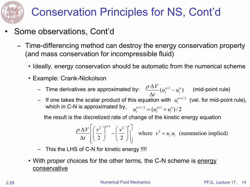
Conservation Principles for NS, Cont’d
• Some observations, Cont’d
– Time-differencing method can destroy the energy conservation property
(and mass conservation for incompressible fluid)
• Ideally, energy conservation should be automatic from the numerical scheme
• Example: Crank-Nickolson
– Time derivatives are approximated by: (mid-point rule)
– If one takes the scalar product of this equation with (vel. for mid-point rule),
which in C-N is approximated by,
the result is the discretized rate of change of the kinetic energy equation
– This the LHS of C-N for kinetic energy !!!!
• With proper choices for the other terms, the C-N scheme is energy
conservative
1( )n ni i
V u ut
1/ 2n
iu
1/ 2 1( ) / 2n n ni i iu u u
12 22where (summation implied)
2 2
n n
i iV v v v u ut

PFJL Lecture 17, 15Numerical Fluid Mechanics2.29
Parabolic PDE: Implicit SchemesLeads to a system of equations to be solved at each time-step
B-C (Backward-Centered):
,
1st order accurate in time,2nd order in space
Unconditionally stable
Crank-Nicolson:2nd order accurate in time
2nd order in space
Unconditionally stable
• Time: centered FD, but evaluated at mid-point
• 2nd derivative in space determined at mid-point by averaging at t and t+1
B-C:• Backward in time • Centered in space
• Evaluates RHS at time t+1 instead of time t (for the explicit scheme)
(review Lecture 14)
tl+1
tl
xi xi+1xi-1
tl+1/2
tl+1
tl
xi xi+1xi-1
Grid point involved in space difference
Grid point involved in time difference
Grid point involved in space difference
Grid point involved in time difference
Simple implicit method
Crank-Nicolson method
Image by MIT OpenCourseWare. After Chapra, S., and R. Canale.Numerical Methods for Engineers. McGraw-Hill, 2005.

PFJL Lecture 17, 16Numerical Fluid Mechanics2.29
Conservation Principles for NS, Cont’d
• Some observations, Cont’d
– Since momentum and kinetic energy (and mass cons.) are not
independent, satisfying all of them is not direct: trial and error in deriving
schemes that are conservative
– Kinetic energy conservation is particularly important in unsteady flows
(e.g. weather, ocean, turbulence, etc)
• Less important for steady flows
– Kinetic energy is not the only quantity whose discrete conservation is
desirable (and not automatic)
• Angular momentum is another one
• Important for flows in rotating machinery, internal combustion engines and
any other devices that exhibit strong rotations/swirl
– If numerical schemes do not conserve these “important” quantities,
numerical simulation is likely to get into trouble, even for stable schemes

PFJL Lecture 17, 17Numerical Fluid Mechanics2.29
Choice of Variable Arrangement on the Grid
• Because the Navier-Stokes equations are coupled equations
for vector fields, several variants of the arrangement of the
computational points/nodes are possible
• Collocated arrangement
– Obvious choice: store all the variables at the same grid points and use
the same grid points or CVs for all variables: Collocated grid
– Advantages:
• All (geometric) coefficients evaluated at the same points
• Easy to apply to multigrid procedures (collocated refinements of the grid)
wWnP e
Ss
N
E
N
W P E
S
ewn
s
Collocated arrangement of velocity components and pressure on FD and FV grids.
Image by MIT OpenCourseWare.

PFJL Lecture 17, 18Numerical Fluid Mechanics2.29
Choice of Variable Arrangement on the Grid
• Collocated arrangement: Disadvantages
– Was out of favor and not used much until the 1980s because of:
• Occurrence of oscillations in the pressure
• Difficulties with pressure-velocity coupling, and requires more interpolations
– However, when non-orthogonal grids started to be used over complex
geometries, the situation changed
• This is because the non-collocated (staggered) approach on non-
orthogonal grids is based on grid-oriented components of the (velocity)
vectors and tensors.
• This implies using curvature terms, which are more difficult to treat numerically and can create non-conservative errors
• Hence, collocated grids became more popular with complex geometries
Variable arrangements on a non-orthogonal grid. Illustrated are a staggered arrangement with (i) contravarient velocity components and (ii) Cartesian velocity components, and (iii) a colocated arrangement with Cartesian velocity components.
Velocities Pressure
(I) (II) (III)
Image by MIT OpenCourseWare.

PFJL Lecture 17, 19Numerical Fluid Mechanics2.29
Choice of Variable Arrangement on the Grid
• Staggered arrangements
– No need for all variables to share the same grid
– “Staggered” arrangements can be advantageous (couples p and v)
• For example, consider the Cartesian coordinates
–Advantages of staggered grids• Several terms that require interpolation
Fully and partially staggered arrangements of velocity components and pressure.
in collocated grids can be evaluated (to 2nd order) without interpolation
• This applies to the pressure term (located at CV centers) and the diffusion term (first derivative needed at CS centers), when obtained by central differences
• Can be shown to directly conserve kinetic energy
• Many variations: partially staggered, etc
N
EW
S
new
s
nw neP
sw se
xi-1 xi
N
EW
S
new
s
nw ne
sw se
xi-1 xi+1xi
N
EW
S
new
s
nw ne
PP
sw se
xi-1
yj-1
yj
yj+1
xi
X
y
Control volumes for a staggered grid for (a) mass conservation and scalar quantities, (b) x-momentum, and (c) y-momentum
(a) (b) (c)
∆
Image by MIT OpenCourseWare.
Image by MIT OpenCourseWare.
PFJL Lecture 17, 20Numerical Fluid Mechanics2.29
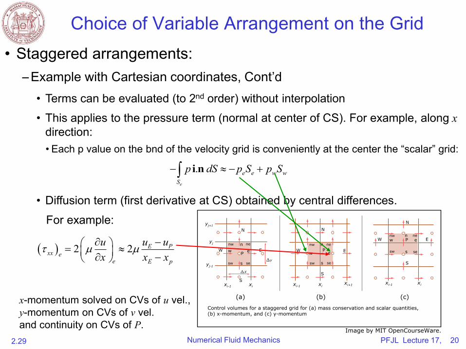
Choice of Variable Arrangement on the Grid
• Staggered arrangements:
– Example with Cartesian coordinates, Cont’d
• Terms can be evaluated (to 2nd order) without interpolation
• This applies to the pressure term (normal at center of CS). For example, along xdirection:• Each p value on the bnd of the velocity grid is conveniently at the center the “scalar” grid:
• Diffusion term (first derivative at CS) obtained by central differences.
For example:
.e
e e w wS
p dS p S p S i n
2 2 E Pxx e
e E p
u u ux x x
x-momentum solved on CVs of u vel., y-momentum on CVs of v vel.and continuity on CVs of P.
N
EW
S
new
s
nw neP
sw se
xi-1 xi
N
EW
S
n
ew
s
nw ne
sw se
xi-1xi+1xi
N
EW
S
new
s
nw ne
PP
sw se
xi-1
yj-1
yj
yj+1
xi
X
y
Control volumes for a staggered grid for (a) mass conservation and scalar quantities, (b) x-momentum, and (c) y-momentum
(a) (b) (c)
Image by MIT OpenCourseWare.

MIT OpenCourseWarehttp://ocw.mit.edu
2.29 Numerical Fluid MechanicsSpring 2015
For information about citing these materials or our Terms of Use, visit: http://ocw.mit.edu/terms.