2.29 numerical fluid mechanics fall 2011 – lecture 20

2.29 Numerical Fluid MechanicsFall 2011 – Lecture 20

REVIEW Lecture 19: Finite Volume Methods – Review: Basic elements of a FV scheme and steps to step-up a FV scheme – One Dimensional examples

xd j x j 1/ 2 x t dx • Generic equation: f j1/ 2 f j1/ 2 s ( , ) xdt j1/ 2

• Linear Convection (Sommerfeld eqn): convective fluxes– 2nd order in space, then 4th order in space, links to CDS

• Unsteady Diffusion equation: diffusive fluxes – Two approaches for 2nd order in space, links to CDS

– Two approaches for the approximation of surface integrals (and volume integrals)– Interpolations and differentiations (express symbolic values at surfaces as a function of nodal variables)

P if v n. 0

e• Upwind interpolation (UDS): e (first-order and diffusive) E if v n. 0 e

x x• Linear Interpolation (CDS): (1 ) where e P (2nd order, can be oscillatory) e E e P e e xE xP E Px x xe E P

g ( ) g ( )e U 1 D U 2 U UU

• Quadratic Upwind interpolation (QUICK) 6 3 1 3 x3 3

R3e U D UU 8 8 8 48 x3 D• Higher order (interpolation) schemes

2.29 Numerical Fluid Mechanics PFJL Lecture 20, 1 1

TODAY (Lecture 20): Time-Marching Methods and ODEs – Initial Value Problems

• Time-Marching Methods and Ordinary Differential Equations – Initial Value Problems

– Euler’s method – Taylor Series Methods

• Error analysis

– Simple 2nd order methods • Heun’s Predictor-Corrector and Midpoint Method

– Runge-Kutta Methods

– Multistep/Multipoint Methods: Adams Methods

– Practical CFD Methods

– Stiff Differential Equations

– Error Analysis and Error Modifiers

– Systems of differential equations

2.29 Numerical Fluid Mechanics PFJL Lecture 20, 22

References and Reading Assignments

• Chapters 25 and 26 of “Chapra and Canale, Numerical Methods for Engineers, 2010/2006.”

• Chapter 6 on “Methods for Unsteady Problems” of “J. H. Ferziger and M. Peric, Computational Methods for Fluid Dynamics. Springer, NY, 3rd edition, 2002”

• Chapter 6 on “Time-Marching Methods for ODE’s” of “H. Lomax, T. H. Pulliam, D.W. Zingg, Fundamentals of Computational Fluid Dynamics (Scientific Computation).Springer, 2003”

• Chapter 5.6 on “Finite-Volume Methods” of T. Cebeci, J. P. Shao, F. Kafyeke and E. Laurendeau, Computational Fluid Dynamics for Engineers. Springer, 2005.


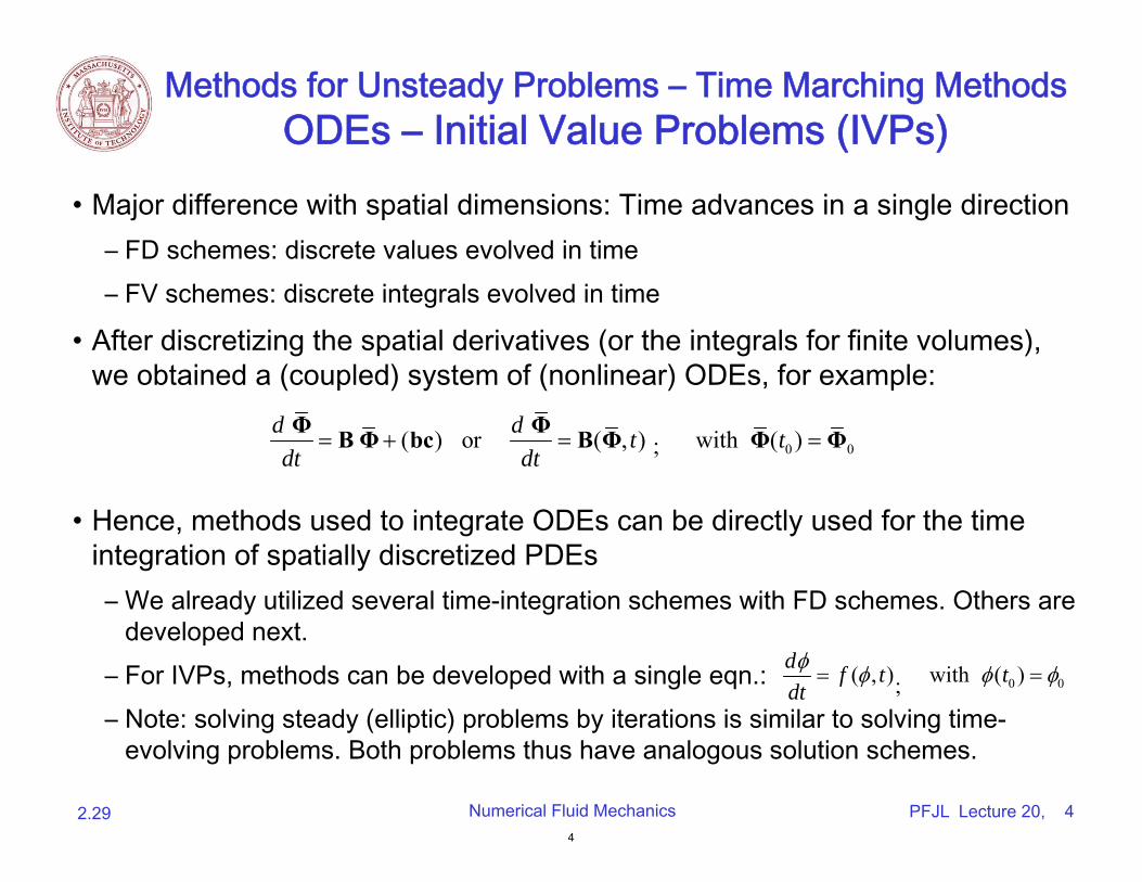
Methods for Unsteady Problems – Time Marching Methods ODEs – Initial Value Problems (IVPs)

• Major difference with spatial dimensions: Time advances in a single direction– FD schemes: discrete values evolved in time – FV schemes: discrete integrals evolved in time

• After discretizing the spatial derivatives (or the integrals for finite volumes), we obtained a (coupled) system of (nonlinear) ODEs, for example:

d Φ d Φ B Φ (bc) or B(Φ t with Φ t0 0, ) ; ( ) Φ

dt dt

• Hence, methods used to integrate ODEs can be directly used for the time integration of spatially discretized PDEs – We already utilized several time-integration schemes with FD schemes. Others are

developed next. – For IVPs, methods can be developed with a single eqn.: d f (, )t ; with ( ) t0 0dt – Note: solving steady (elliptic) problems by iterations is similar to solving time-

evolving problems. Both problems thus have analogous solution schemes.


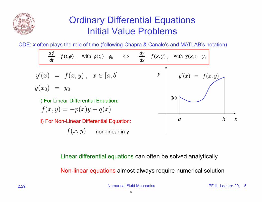
Ordinary Differential EquationsInitial Value Problems

ODE: x often plays the role of time (following Chapra & Canale’s and MATLAB’s notation)

y

0 0 0 0( , ) ; with ( ) ( , ) ; with y( )d dy f t t f x y x ydt dx

non-linear in y

ii) For Non-Linear Differential Equation:

i) For Linear Differential Equation:

a b x

Linear differential equations can often be solved analytically

Non-linear equations almost always require numerical solution


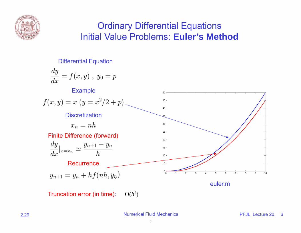
Ordinary Differential EquationsInitial Value Problems: Euler’s Method

Differential Equation

Example

Discretization

Finite Difference (forward)

Recurrence

euler.m

Truncation error (in time): O(h2)


(from Lecture 1)

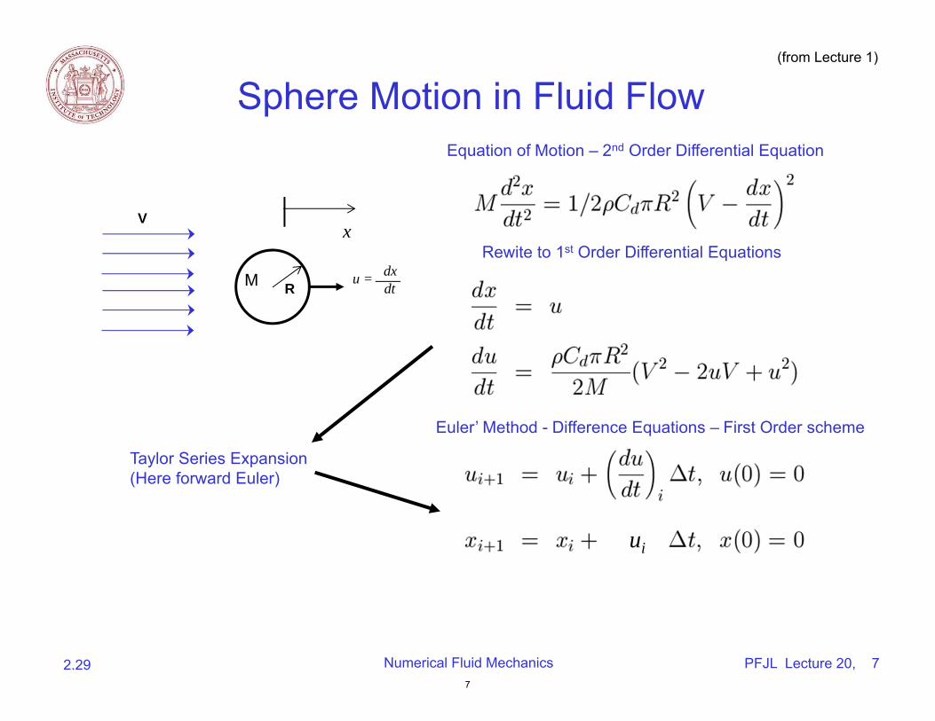
Sphere Motion in Fluid Flow Equation of Motion – 2nd Order Differential Equation

V x

RM dx u = dt

Taylor Series Expansion (Here forward Euler)

Rewite to 1st Order Differential Equations

Euler’ Method - Difference Equations – First Order scheme

ui


(from Lecture 1)

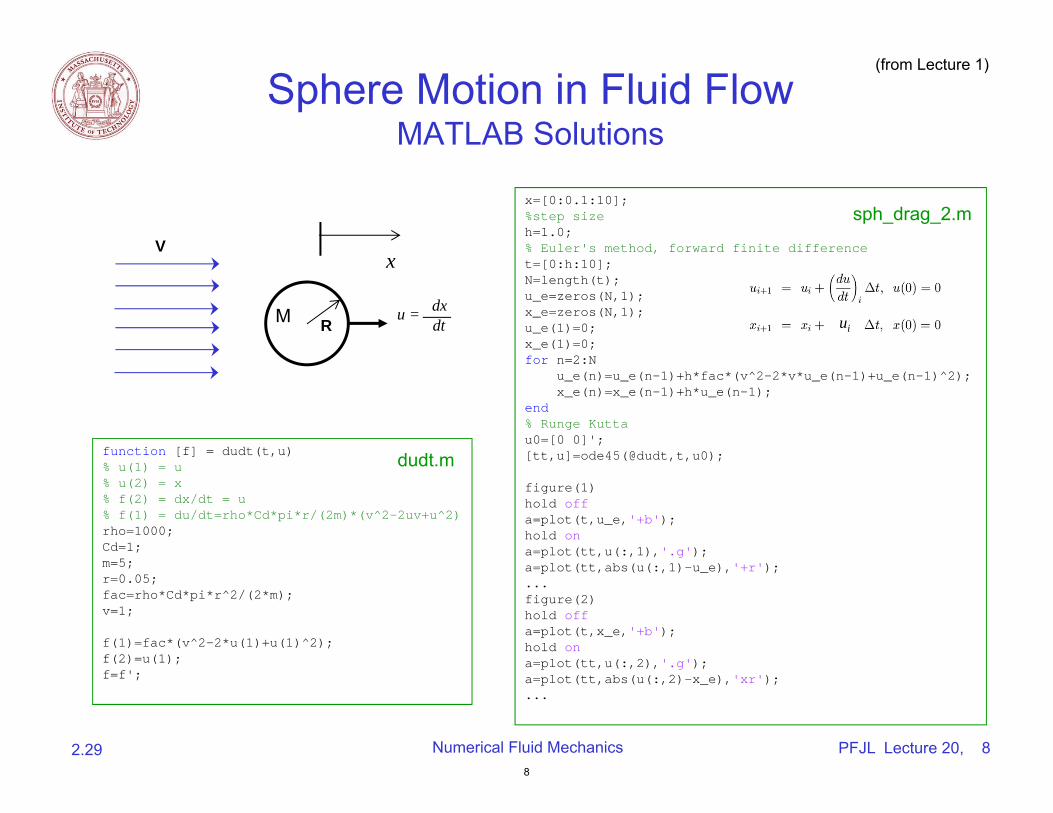
Sphere Motion in Fluid Flow MATLAB Solutions

V x

RM dx u = dt

function [f] = dudt(t,u)% u(1) = u% u(2) = x% f(2) = dx/dt = u% f(1) = du/dt=rho*Cd*pi*r/(2m)*(v^2-2uv+u^2)rho=1000;Cd=1;m=5;r=0.05;fac=rho*Cd*pi*r^2/(2*m);v=1;

f(1)=fac*(v^2-2*u(1)+u(1)^2);f(2)=u(1);f=f';

dudt.m

x=[0:0.1:10];%step sizeh=1.0;% Euler's method, forward finite differencet=[0:h:10];N=length(t);u_e=zeros(N,1);x_e=zeros(N,1);u_e(1)=0;x_e(1)=0;for n=2:N

u_e(n)=u_e(n-1)+h*fac*(v^2-2*v*u_e(n-1)+u_e(n-1)^2);x_e(n)=x_e(n-1)+h*u_e(n-1);

end % Runge Kuttau0=[0 0]';[tt,u]=ode45(@dudt,t,u0);

figure(1)hold off a=plot(t,u_e,'+b');hold on a=plot(tt,u(:,1),'.g');a=plot(tt,abs(u(:,1)-u_e),'+r'); ... figure(2)hold off a=plot(t,x_e,'+b');hold on a=plot(tt,u(:,2),'.g');a=plot(tt,abs(u(:,2)-x_e),'xr'); ...

sph_drag_2.m

ui


(from Lecture 1)

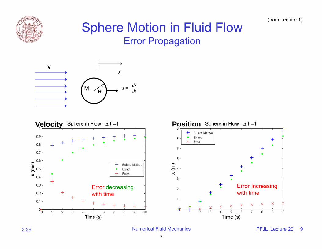
Sphere Motion in Fluid Flow Error Propagation

V x

dx u = dtRM

Error Increasing with time

Error decreasing with time

Velocity Position


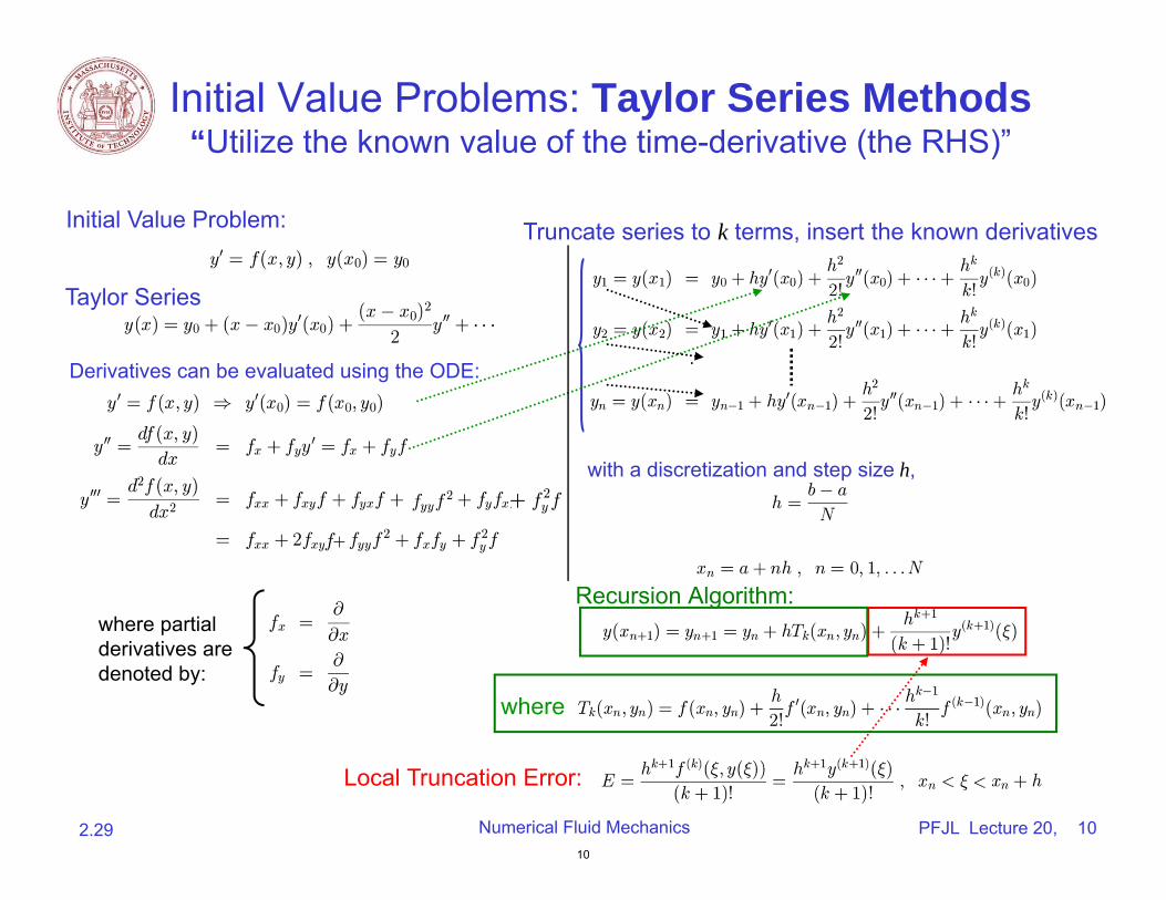
Initial Value Problems: Taylor Series Methods “Utilize the known value of the time-derivative (the RHS)”

Taylor Series

where partial derivatives are denoted by:

Derivatives can be evaluated using the ODE:

+

Truncate series to k terms, insert the known derivatives Initial Value Problem:

with a discretization and step size h,

Recursion Algorithm:

where

Local Truncation Error:

+


Initial Value Problems: Taylor Series Methods

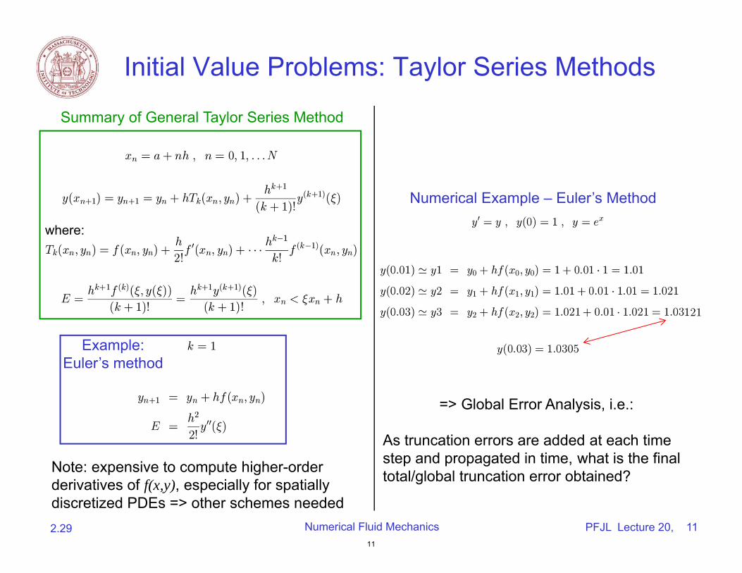
Summary of General Taylor Series Method

Example: Euler’s method

where:

Note: expensive to compute higher-order derivatives of f(x,y), especially for spatially discretized PDEs => other schemes needed

Numerical Example – Euler’s Method

=> Global Error Analysis, i.e.:

As truncation errors are added at each time step and propagated in time, what is the final total/global truncation error obtained?


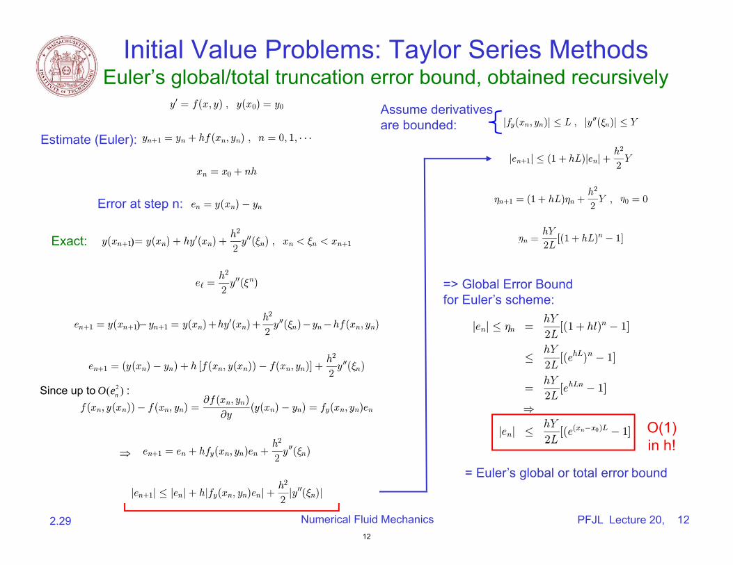
Initial Value Problems: Taylor Series MethodsEuler’s global/total truncation error bound, obtained recursively

Assume derivatives are bounded:

=> Global Error Bound Euler’s

Truncation error

)Exact:

Estimate (Euler):

)

Error at step n:

Since up to :

2( )nO e


O(1) in h!

for Euler’s scheme:

= Euler’s global or total error bound

12

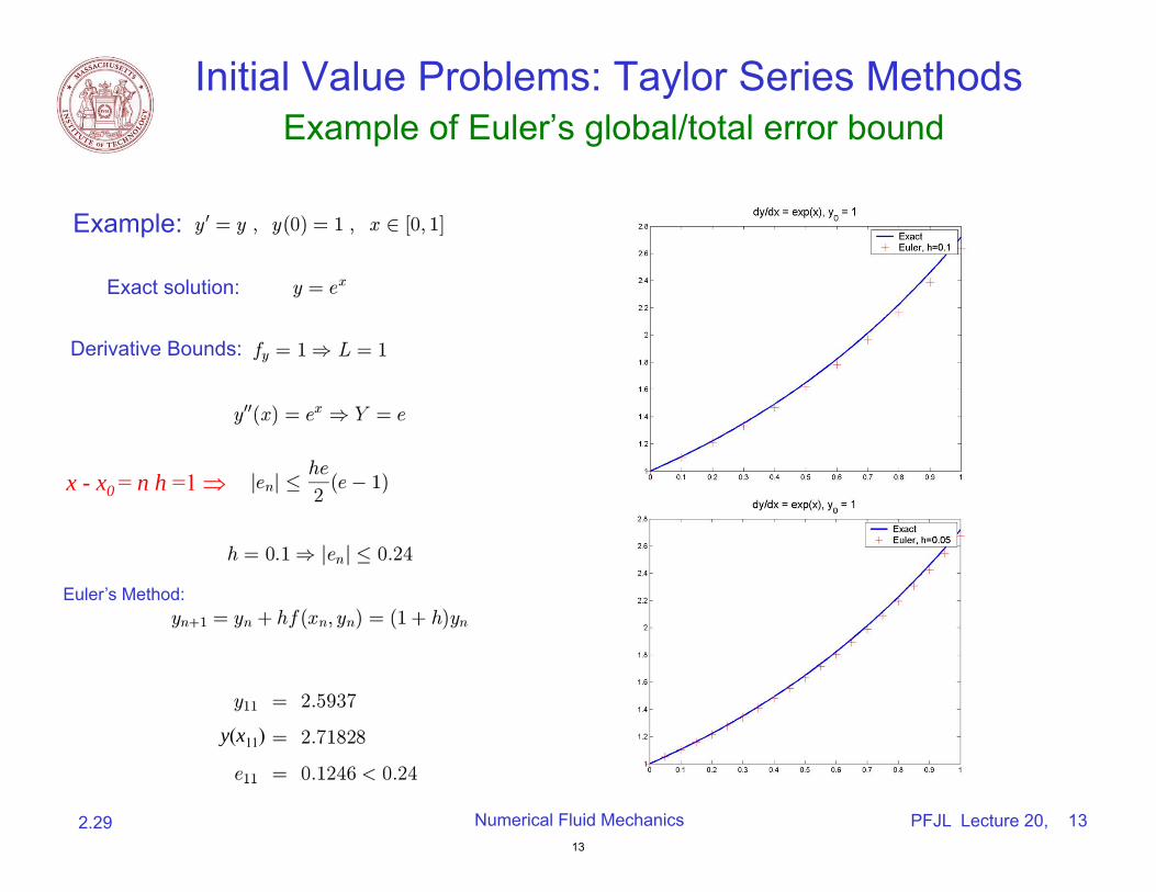
Initial Value Problems: Taylor Series MethodsExample of Euler’s global/total error bound

Example:

Exact solution:

Derivative Bounds:

x - x0 = n h =1

y(x11)

Euler’s Method:


Improving Euler’s Method

• For one-step (two-time levels) methods, the global error result for Euler can be generalized to any method of nth order: – If the truncation error is of O(hn), the global error is of O(hn-1)

• Euler’s method assumes that the (initial) derivative applies to the whole time interval => 1st order global error

• Two simple methods modify Euler’s method by estimating the derivatives within the time-interval – Heun’s method – Midpoint rule

• The intermediate estimates of the derivative lead to 2nd order global errors • Heun’s and Midpoint methods belong to the general class of Runge-Kutta

methods – introduced now since they are also linked to classic PDE integration schemes


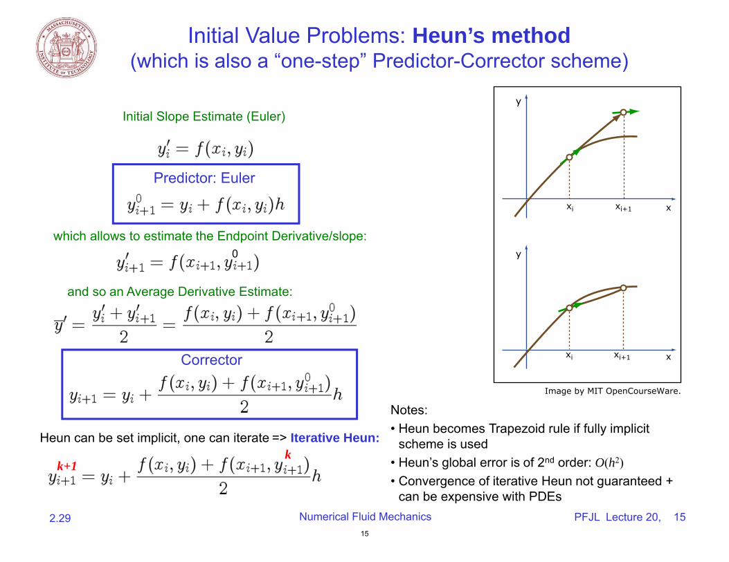
Initial Value Problems: Heun’s method which is also a “one-step” Predictor-Corrector scheme)(

Initial Slope Estimate (Euler)

Predictor: Euler

which allows to estimate the Endpoint Derivative/slope:

and so an Average Derivative Estimate:

Corrector

0

Notes: • Heun becomes Trapezoid rule if fully implicit

scheme is used • Heun’s global error is of 2nd order: O(h2)• Convergence of iterative Heun not guaranteed +

can be expensive with PDEs

Heun can be set implicit, one can iterate => Iterative Heun: k

k+1


xi xi+1

y

x

xi xi+1

y

x

Image by MIT OpenCourseWare.

nkum43

Line

nkum43

Line

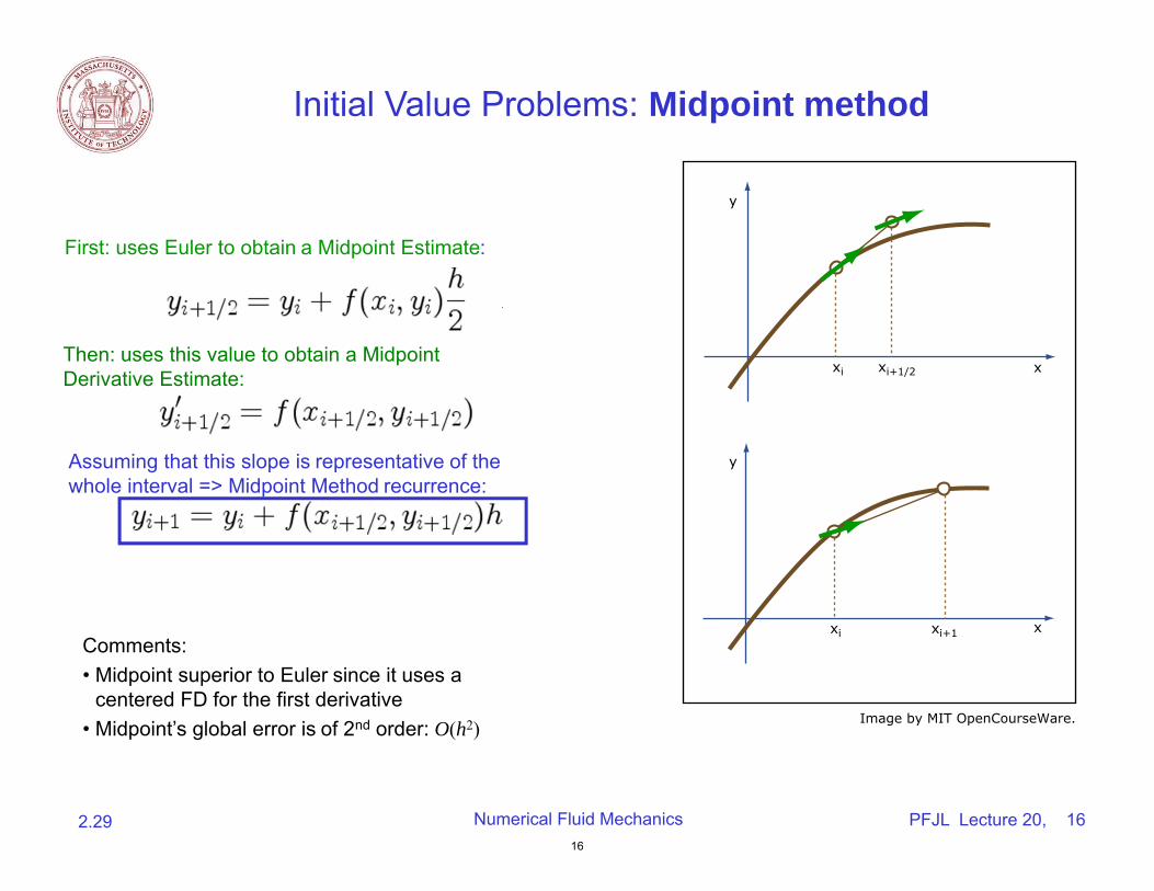
Initial Value Problems: Midpoint method

First: uses Euler to obtain a Midpoint Estimate:

Then: uses this value to obtain a Midpoint Derivative Estimate:

Assuming that this slope is representative of the whole interval => Midpoint Method recurrence:

Comments: • Midpoint superior to Euler since it uses a

centered FD for the first derivative • Midpoint’s global error is of 2nd order: O(h2)


xi

xi

xi+1/2

xi+1

y

y

x

x


ndhami

Line

ndhami

Line

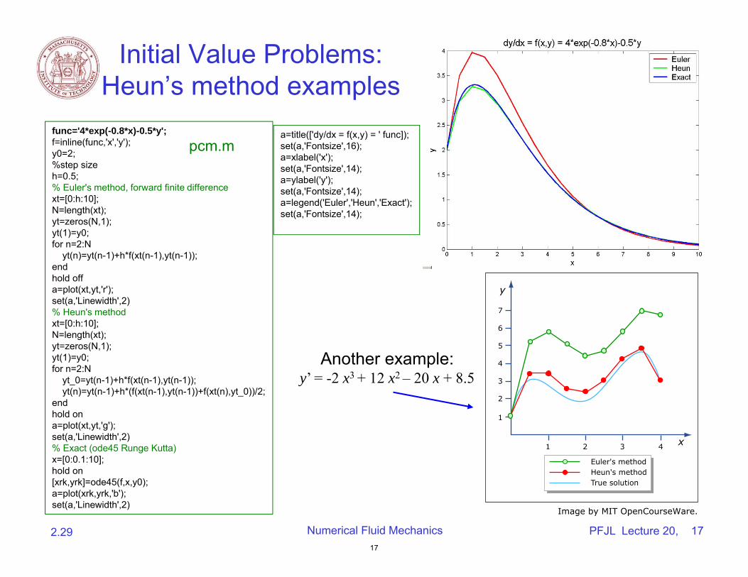
Initial Value Problems: Heun’s method examples

func='4*exp(-0.8*x)-0.5*y'; f=inline(func,'x','y'); y0=2; %step size h=0.5; % Euler's method, forward finite difference xt=[0:h:10]; N=length(xt); yt=zeros(N,1); yt(1)=y0; for n=2:N

yt(n)=yt(n-1)+h*f(xt(n-1),yt(n-1)); end hold off a=plot(xt,yt,'r'); set(a,'Linewidth',2) % Heun's method xt=[0:h:10]; N=length(xt); yt=zeros(N,1); yt(1)=y0; for n=2:N

yt_0=yt(n-1)+h*f(xt(n-1),yt(n-1)); yt(n)=yt(n-1)+h*(f(xt(n-1),yt(n-1))+f(xt(n),yt_0))/2;

end hold on a=plot(xt,yt,'g'); set(a,'Linewidth',2) % Exact (ode45 Runge Kutta) x=[0:0.1:10]; hold on [xrk,yrk]=ode45(f,x,y0); a=plot(xrk,yrk,'b'); set(a,'Linewidth',2)

a=title(['dy/dx = f(x,y) = ' func]); pcm.m set(a,'Fontsize',16);

a=xlabel('x'); set(a,'Fontsize',14); a=ylabel('y'); set(a,'Fontsize',14); a=legend('Euler','Heun','Exact'); set(a,'Fontsize',14);

Another example: y’ = -2 x3 + 12 x2 – 20 x + 8.5

1

1

2

2

3

3 4

4

5

6

7

y

x

True solutionHeun's methodEuler's method

17



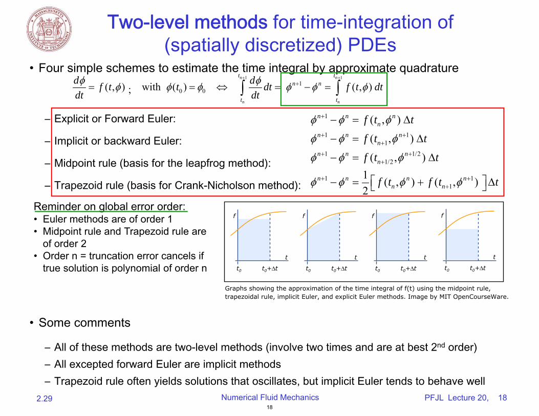
Two-level methods for time-integration of (spatially discretized) PDEs

• Four simple schemes to estimate the time integral by approximate quadraturen 1 n 1d t d n1 n

t

( , t ) ; with t0 0 dt f ( , ) f ( ) t dt dt dttn tn

Reminder on global error order: • Euler methods are of order 1 • Midpoint rule and Trapezoid rule are

of order 2• Order n = truncation error cancels if

true solution is polynomial of order n

– Explicit or Forward Euler:

– Implicit or backward Euler:

– Midpoint rule (basis for the leapfrog method):

– Trapezoid rule (basis for Crank-Nicholson method):

1

1 1 1

1 1/2 1/2

1 1 1

)

( , )

( , ) 1 ( , ) ( , )2

n n n n

n n n n

n n n n

n n n n n n

t

f t t

( ,f t

f t t

f t f t t

• Some comments

– All of these methods are two-level methods (involve two times and are at best 2nd order) – All excepted forward Euler are implicit methods

– Trapezoid rule often yields solutions that oscillates, but implicit Euler tends to behave well 2.29 Numerical Fluid Mechanics PFJL Lecture 20, 18

18

f

t0 t0+∆t

t

f

t0 t0+∆t

t

f

t0 t0+∆t

t

f

t0 t0+∆t

t

Graphs showing the approximation of the time integral of f(t) using the midpoint rule, trapezoidal rule, implicit Euler, and explicit Euler methods. Image by MIT OpenCourseWare.

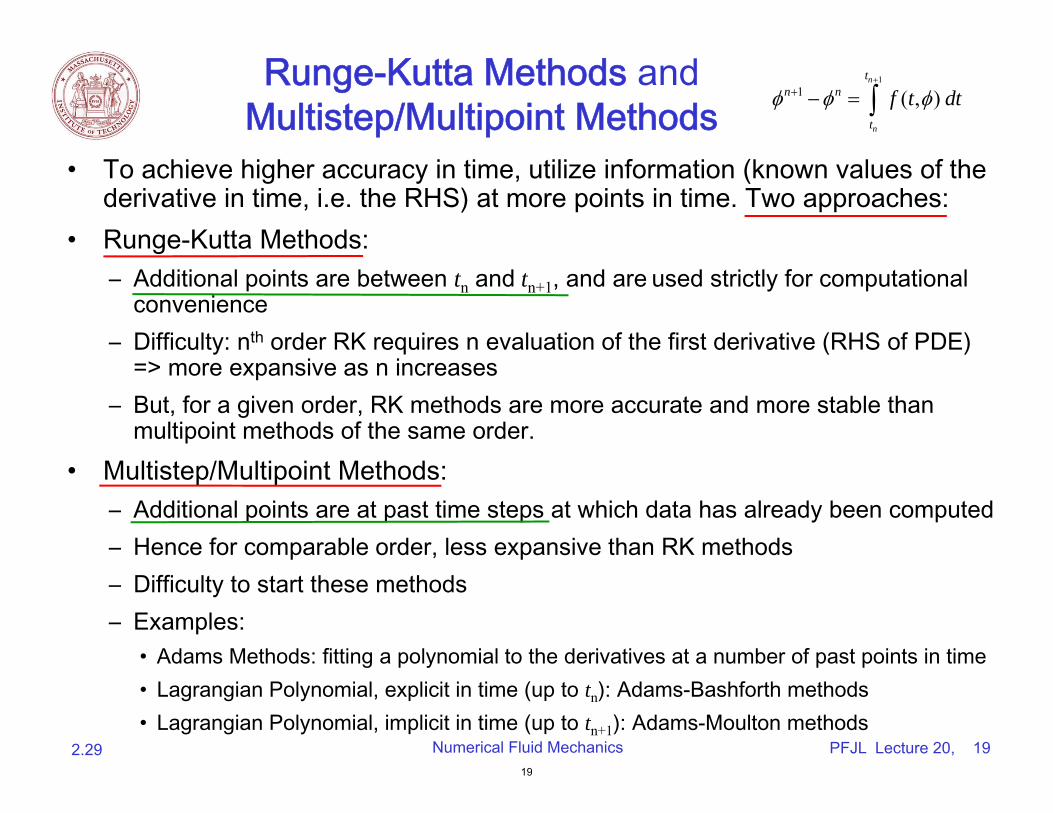
tn1Runge-Kutta Methods and n1 n f ( , ) t dt Multistep/Multipoint Methods tn

• To achieve higher accuracy in time, utilize information (known values of the derivative in time, i.e. the RHS) at more points in time. Two approaches:

• Runge-Kutta Methods: –Additional points are between tn and tn+1, and are used strictly for computational

convenience –Difficulty: nth order RK requires n evaluation of the first derivative (RHS of PDE)

=> more expansive as n increases –But, for a given order, RK methods are more accurate and more stable than

multipoint methods of the same order. • Multistep/Multipoint Methods:

–Additional points are at past time steps at which data has already been computed –Hence for comparable order, less expansive than RK methods –Difficulty to start these methods –Examples:

• Adams Methods: fitting a polynomial to the derivatives at a number of past points in time • Lagrangian Polynomial, explicit in time (up to tn): Adams-Bashforth methods • Lagrangian Polynomial, implicit in time (up to tn+1): Adams-Moulton methods


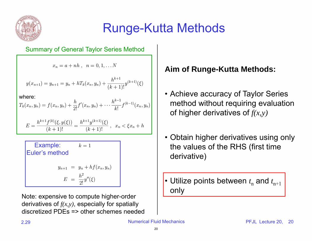
Runge-Kutta MethodsSummary of General Taylor Series Method

Example: Euler’s method

where:

Note: expensive to compute higher-order derivatives of f(x,y), especially for spatially discretized PDEs => other schemes needed

Aim of Runge-Kutta Methods:

• Achieve accuracy of Taylor Series method without requiring evaluation of higher derivatives of f(x,y)

• Obtain higher derivatives using only the values of the RHS (first time derivative)

• Utilize points between tn and tn+1 only


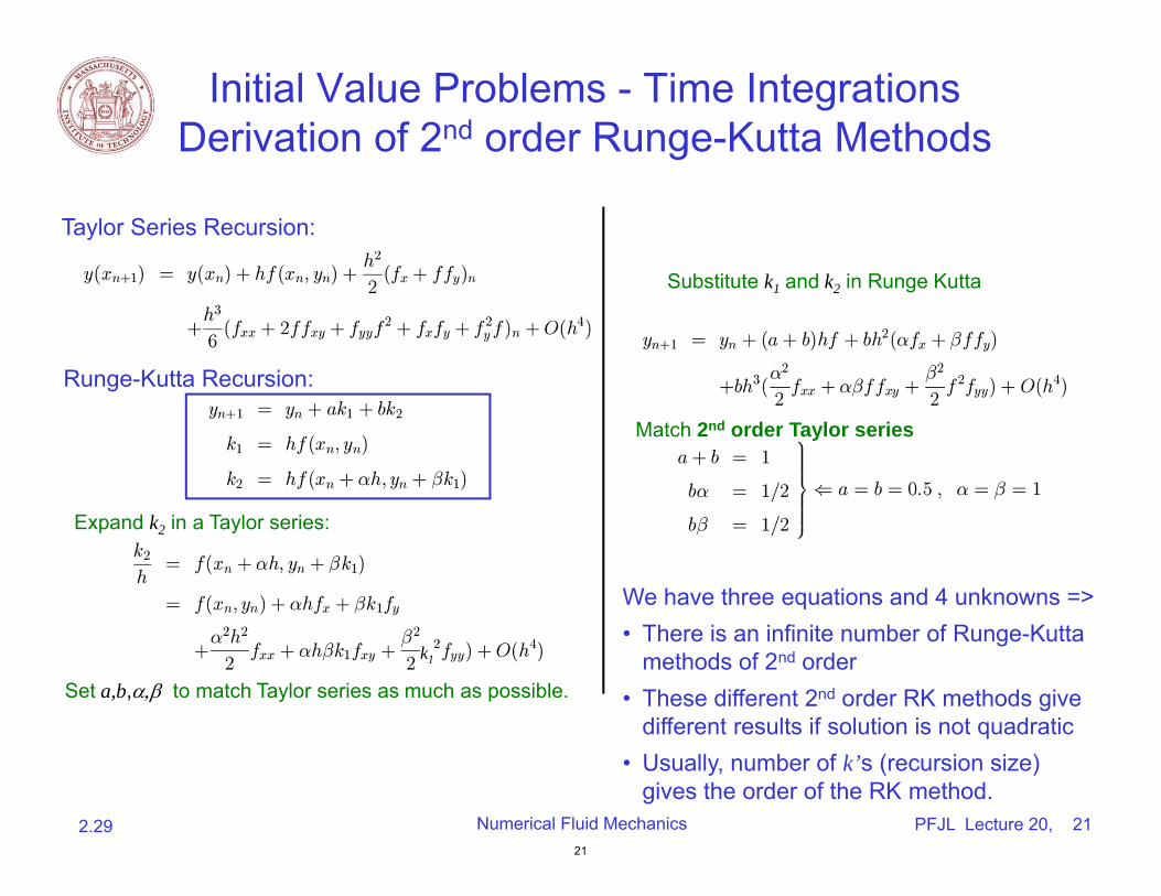
Initial Value Problems - Time IntegrationsDerivation of 2nd order Runge-Kutta Methods

Taylor Series Recursion:

Runge-Kutta Recursion:

Set a,b, to match Taylor series as much as possible.

Expand k2 in a Taylor series:

k1

Substitute k1 and k2 in Runge Kutta

Match 2nd order Taylor series

We have three equations and 4 unknowns => • There is an infinite number of Runge-Kutta

methods of 2nd order • These different 2nd order RK methods give

different results if solution is not quadratic • Usually, number of k’s (recursion size)

gives the order of the RK method. 2.29 Numerical Fluid Mechanics PFJL Lecture 20, 21

21

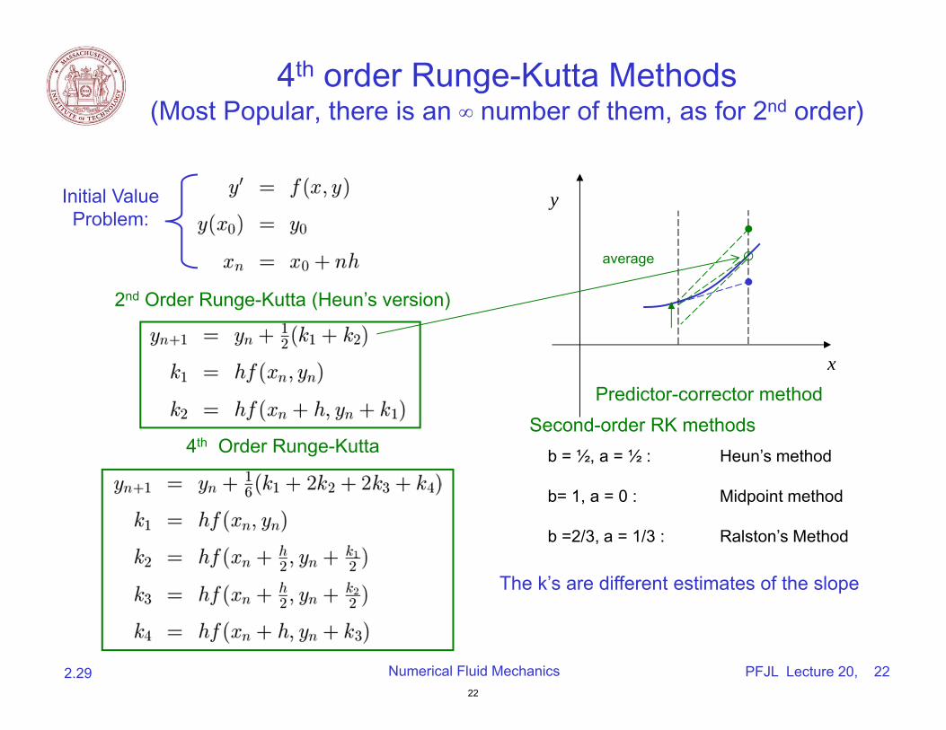
4th order Runge-Kutta Methods(Most Popular, there is an ∞ number of them, as for 2nd order)

x Predictor-corrector method

Second-order RK methods b = ½, a = ½ : Heun’s method

b= 1, a = 0 : Midpoint method

b =2/3, a = 1/3 : Ralston’s Method

The k’s are different estimates of the slope

Initial Value Problem:

2nd Order Runge-Kutta (Heun’s version)

4th Order Runge-Kutta

y

average


PFJL Lecture 20,

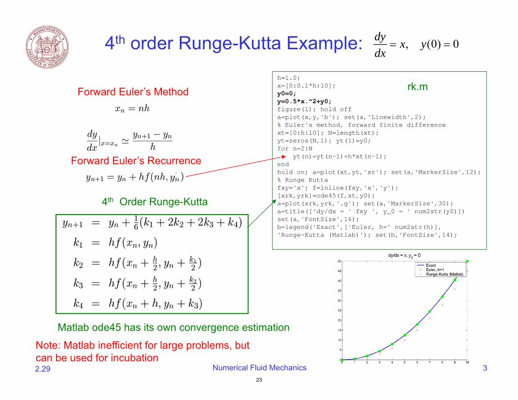
Forward Euler’s Method

Forward Euler’s Recurrence

4th Order Runge-Kutta

Matlab ode45 has its own convergence estimation

Note: Matlab inefficient for large problems, but can be used for incubation 2.29 Numerical Fluid Mechanics 23

4th order Runge-Kutta Example: dy x, y(0) 0

dx

h=1.0;x=[0:0.1*h:10]; rk.my0=0;y=0.5*x.^2+y0;figure(1); hold off a=plot(x,y,'b'); set(a,'Linewidth',2); % Euler's method, forward finite difference xt=[0:h:10]; N=length(xt); yt=zeros(N,1); yt(1)=y0; for n=2:N

yt(n)=yt(n-1)+h*xt(n-1);end hold on; a=plot(xt,yt,'xr'); set(a,'MarkerSize',12);% Runge Kuttafxy='x'; f=inline(fxy,'x','y');[xrk,yrk]=ode45(f,xt,y0);a=plot(xrk,yrk,'.g'); set(a,'MarkerSize',30);a=title(['dy/dx = ' fxy ', y_0 = ' num2str(y0)])set(a,'FontSize',16);b=legend('Exact',['Euler, h=' num2str(h)],'Runge-Kutta (Matlab)'); set(b,'FontSize',14);

23

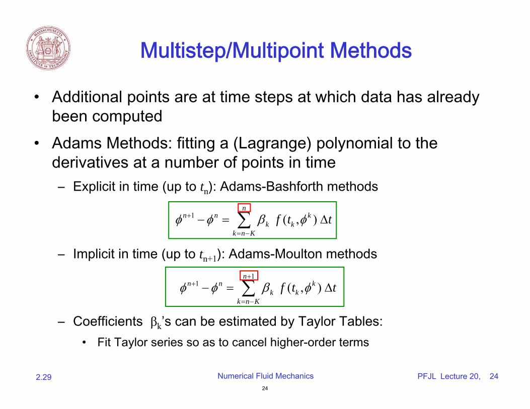
Multistep/Multipoint Methods

• Additional points are at time steps at which data has already been computed

• Adams Methods: fitting a (Lagrange) polynomial to the derivatives at a number of points in time –Explicit in time (up to tn): Adams-Bashforth methods

1 ( , ) n

n n k k k

k n K

f t t

– Implicit in time (up to tn+1): Adams-Moulton methods 1

1 ( , ) n

n n k k k

k n K

f t t

– Coefficients βk’s can be estimated by Taylor Tables:

• Fit Taylor series so as to cancel higher-order terms


MIT OpenCourseWarehttp://ocw.mit.edu

2.29 Numerical Fluid Mechanics Fall 2011

For information about citing these materials or our Terms of Use, visit: http://ocw.mit.edu/terms.

http://ocw.mit.edu

http://ocw.mit.edu/terms

2.29 numerical fluid mechanics fall 2011 – lecture 20

Documents