2019 spring prof. d. j. lee, snu

Engineering Economic Analysis2019 SPRING

Prof. D. J. LEE, SNU

Chap. 5

CHOICE

Economic Rationality

§ The principal behavioral postulate is that a decision maker chooses its most preferred alternative from those available to it.

§ Utility maximization with budget constraint

1

Optimal Choice

Affordablebundles

x1

x2

More preferredbundles

2

Optimal Choice

x1

x2

x1*

x2*

(x1*,x2*) is the mostpreferred affordablebundle.

3

Optimal Choice

x1

x2

x1*

x2*

Note that x1*>0, x2*>0 (Interior solution) I.C. is tangent to budget line

4

Optimal Choice

§ (x1*,x2*) satisfies two conditions:• the budget is exhausted;

p1x1* + p2x2* = m• the slope of the budget constraint, -p1/p2, and the

slope of the indifference curve containing (x1*,x2*) are equal at (x1*,x2*).

* *2 1 11 2

1 2 2

at ( , )dx MU pMRS x x

dx MU p= = =

§ Are these conditions always hold at the optimal choice? (Necessary & sufficient condition?)

5

Optimal Choice

§ Kinky tastes

§ I.C. has a kink at (x1*,x2*), there is no tangency!

6

Optimal Choice

§ Boundary optimum (corner solution): optimal point occurs where some xi*=0

§ No tangency since * *11 2

2

at ( , )pMRS x x

p¹

7

Optimal Choice

§ By ruling out the kinky case (non-differentiable case),

§ Necessary condition of the optimal choice: If the optimal choice is an interior point, then necessarily the I.C. will be tangent to the budget line

§ Sufficiency?

8

Optimal Choice

§ No convex case

Tangent but not optimal !

§ In general, the tangency condition is only a necessary condition for optimality, not a sufficient one

9

Optimal Choice

§ However, the convex preference is the case where the tangency condition is sufficient

§ Uniqueness?

§ If the I.C.s are strictly convex, then there will be only one optimal choice on each budget line

10

Optimal Choice

§ Economic meaning of tangency condition

11

* *2 1 11 2

1 2 2

at ( , )dx MU pMRS x x

dx MU p= = =

• MRS = the rate of change at which the consumer is just willing to substitute

• p1/p2 = the rate of change the consumer can do in the market

• If MRS> p1/p2 → p2dx2>p1dx1 → Buy x1 more! and vice versa

• Thus at MRS = p1/p2, there will be no more exchange• Consumer equilibrium condition

Utility maximization & Demand function

§ Utility maximization problem

12

( ). .

, n

Max u xs t p x m

x X p R+

× £

Î Î

§ Demand function• the solution of ‘Utility maximization problem’• The function that relates the optimal choice to the

different values of prices and income*

1( ,..., , ) for 1,...,j nx p p m j n=


§ Two-good case with equality constraint

13

1 21 2,

1 1 2 2

max ( , )

. .x xU x x

s t p x p x m+ =

• Lagrangian function1 2 1 1 2 2( , ) ( )L u x x p x p x ml= - + -

• First-order conditions (F.O.C.)* *1 2

11 1

* *1 2

22 2

* *1 1 2 2

( , )0 (1)

( , )0 (2)

0 (3)

u x xLp

x x

u x xLp

x xL

m p x p x

l

l

l

ì ¶¶= - =ï ¶ ¶ï

ï ¶¶ï = - =í¶ ¶ïï ¶

= - - =ï¶ïî

*1 1 1 2*2 2 1 2

( , , )( , , )

x x p p mx x p p m

ì =ïí

=ïî

• Optimal choice: demand function


§ Consumer equilibrium condition• By Eq. (1) & (2),

14

1 2

1 2

1 1

2 2

MU MUp p

MU p MRSMU p

l = =

\ = =


15

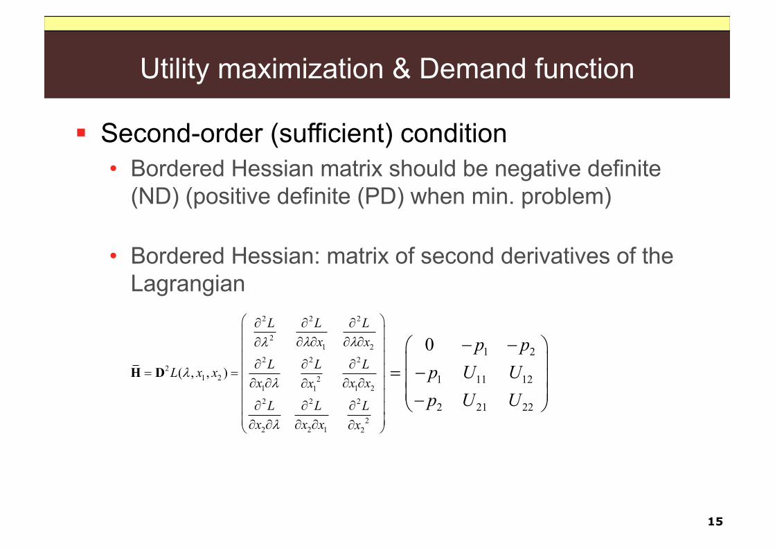
§ Second-order (sufficient) condition• Bordered Hessian matrix should be negative definite

(ND) (positive definite (PD) when min. problem)

• Bordered Hessian: matrix of second derivatives of the Lagrangian

2 2 2

21 2

2 2 22

1 2 21 1 212 2 2

22 2 1 2

( , , )

L L Lx x

L L LL x x

x x xx

L L Lx x x x

l ll

ll

l

æ ö¶ ¶ ¶ç ÷

¶ ¶ ¶ ¶¶ç ÷ç ÷¶ ¶ ¶ç ÷= =¶ ¶ ¶ ¶¶ç ÷

ç ÷¶ ¶ ¶ç ÷

ç ÷¶ ¶ ¶ ¶ ¶è ø

H D

1 2

1 11 12

2 21 22

0 p pp U Up U U

- -æ öç ÷= -ç ÷ç ÷-è ø


16

1 2

1 11 12

2 21 22

0det( ) 0

p pp U Up U U

- -= - >-

H

• ND: naturally ordered principal minors must alternate in sign starting from (-) to (+) to (-) …..

• PD: naturally ordered principal minors must have the same sign of (-1)k , where k is the number of constraints

Examples: Cobb-Douglas

• By monotonic transformation,

17

1 2 1 2( , ) c du x x x x=

1 2 1 2ln ( , ) ln lnu x x c x d x= +

• Utility max. problem; 1 2

1 1 2 2

max ln ln. .

c x d xs t p x p x m

++ =

• Lagrangian;

1 2 1 1 2 2ln ln ( )L c x d x p x p x ml= + - + -

• F.O.C. 1

1 1

22 2

1 1 2 2

0 (1)

0 (2)

0 (3)

L cp

x xL d

px xL

m p x p x

l

l

l

¶ì = - =ï¶ïï ¶

= - =í¶ï

ï ¶= - - =ï

¶î

Examples: Cobb-Douglas

• Demand function

18

*1 1 2

1

*2 1 2

2

( , , )

( , , )

c mx p p m

c d pd m

x p p mc d p

ì = ×ï +ïíï = ×ï +î

• To check S.O.C.

1 22

1 12

2 2

0/ 00 /

p pp c xp d x

- -æ öç ÷= - -ç ÷ç ÷- -è ø

H 2 22 1 1 2( / ) ( / ) 0c p x d p x= + >H

ND !!

Examples: Perfect substitutes

19

x1

x2

MRS = -a/b

p1/p2 < a/b

p1/p2 > a/b

* * 11 2

1 2

* * 11 2

2 2

* * 11 1 2 2

2

, 0

0,

pm ax x if

p b ppm a

x x ifp b p

pap x p x m if

b p

ì= = >ï

ïïï = = <íïï

+ = =ïïî

p1/p2 = a/b

§ Boundary solution case

Examples: Perfect complements

20

x1

x2

bx2 = ax1

p1x1 + p2x2 = m

* *1 2

1 2 1 2

, mb max x

bp ap bp ap= =

+ +

Examples: Concave preference

21

2 21 2 1 2( , )u x x x x= +

x1

x2

The most preferredaffordable bundle

Tangency point

Better

§ Boundary solution case• Tangency point is not

optimal• Not meet S.O.C.

Choosing taxes

§ If the government wants to raise a certain amount of

revenue, is it better to raise it via quantity tax or an

income tax?

22

§ Imposition of quantity tax on good 1 with a rate t

• Budget constraint changes with price increase from p1 to (p1 +t)

• Let (x1*, x2*) be the optimal choice under the new budget set

• Then we know that (p1+t)x1* + p1x2* =m and tax revenue=tx1*

§ Imposition of income tax which raises the same amount of

tax revenue

• Budget constraint changes with income decrease from m to m-tx1*

Choosing taxes

x2

x1

x2*

x1* x1’

• Optimal choice with quantity tax: (x1*, x2*)

x2’

• Optimal choice with income tax of the same tax revenue: (x1’, x2’)

• (x1’, x2’) ≻(x1*, x2*)

§ Income tax is superior to the quantity tax !

Indirect utility function/ Expenditure function

§ Utility maximization problem

24

( ). .

, n

Max u xs t p x m

x X p R+

× =

Î Î

§ Local non-satiation preference 0,

Given any x in X and any

then there is some bundle y in X with x y such that y x

ee

>

- <

§ Under the local non-satiation assumption, a utility-max. bundle must meet the budget constraint with equality.

Indirect utility function/ Expenditure function

§ Indirect utility function• The max. utility achievable at given prices and income

25

( , ) ( ) . . v p m Max u x

s t p x m=

× =

§ Expenditure function• Inverse of indirect utility function w.r.t. income m

( , )m e p u=

• the minimal amount of income necessary to achieve utility u at p

( , ) min. . ( )

e p u p xs t u x u= ×

³

Hicksian demand function

§ Hicksian demand function:• Expenditure-minimizing bundle necessary to achieve

utility level u at prices

26

p

( , )ih p u

( , )( , )ii

e p uh p up

¶=

¶* *

*

Let be a expenditure-minimizing bundle that gives utility at prices . Then define the function,

Since , is the cheapest way to achieve , this

)

) ( ) ( , )

(

Proof h u p

hg p e pe p u u

u p= - ×

* *

* **

function is always nonpositive. At , ( ) 0. Since this is a maximum value of , its derivative must be zero by F.O.C.:

( )

( )

( 0 1,...,, )i

i i

g p

e

p p g p

g ph i n

pu

pp

= =

¶ ¶= - = =

¶ ¶

Note that ( , ) :Marshallian demand functionix p m

Some important identities

§ Utility max.

27

max ( )

. .xu x

s t p x m× =

*( , ) :Marshallian demand functionix p m ( ),v p m u=

§ Expenditure min. min. . ( )p x

s t u x u×³

*( , ): Hicksian demand functionih p u ( ),e p u m=

Some important identities

28

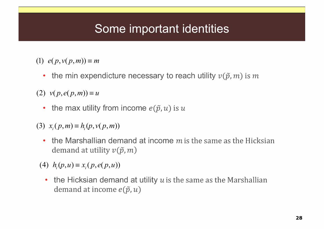
(1) ( , ( , ))e p v p m mº

(2) ( , ( , ))v p e p m uº

(3) ( , ) ( , ( , ))i ix p m h p v p mº

(4) ( , ) ( , ( , ))i ih p u x p e p uº

Roy’s identity

§ Utility max.

29

max ( )

. .xu x

s t p x m× =



s t u x u×³


Inverse

( , )( , )ii

e p uh p up

¶=

¶

?Roy’s identity

Roy’s identity

§ Roy’s identity

30

( ) ( )( )

, /, when 0, 0

, /i

i i

v p m px p m p m

v p m m¶ ¶

= - > >¶ ¶

( ) ( )( ) 1The indirect utility funcion is given by , , , where ( ,..., )nv p m u x p m x x xº =

• Proof

( )1

, ( )If we differnetiate this w.r.t , we find n

ij

ij i j

v p m xu xp

p x p=

¶ ¶¶= ×

¶ ¶ ¶å

( )

( )1

( )Since , satisfies F.O.C. for utility max such that 0,

, (1)

ii

ni

iij j

u xx p m p

x

v p m xp

p p

l

l=

¶- =

¶

¶ ¶=

¶ ¶å

( ) ( )

( )1

And also , satisfies the budget constraint, ,

Differentiating this identity w.r.t. gives , 0 (2)n

ij j i

i j

x p m p x p m m

xp x p m p

p=

× º

¶+ =

¶å

Roy’s identity

31

( ) ( ),Substitute (2) into (1), ,j

j

v p mx p m

pl

¶= -

¶

( ) ( ) ( )( )( )

1

1 1

Now we differentiate , , ,..., , w.r.t. to find

, ( ) (3)

n

n ni i

ii ii

v p m u x p m x p m m

v p m x xu xp

m x m ml

= =

º

¶ ¶ ¶¶= × =

¶ ¶ ¶ ¶å å

( )

1

Differnetiating , w.r.t. , we have

1 (4)n

ii

i

p x p m m m

xpm=

× º

¶=

¶å

( )Substituting (4) into (3) gives us

, v p mm

l¶

=¶

( ) ( ),Finally, , /j

j

v p mx p m

pl

¶= - =

¶( )( ), /, /

jv p m pv p m m¶ ¶

-¶ ¶

Utility max. vs. Expenditure min.

§ Utility max.

32

max ( )

. .xu x

s t p x m× =



s t u x u×³


Inverse

( , )( , )ii

e p uh p up

¶=

¶

( ) ( )( ), /

,, /

ii

v p m px p m

v p m m¶ ¶

= -¶ ¶

Examples

§ Cobb-Douglas utility

33

2019 spring prof. d. j. lee, snu

Documents