2019 introduction to numerical analysiskfjack/lecture/... · introduction to numerical analysis ......

INTRODUCTION TO NUMERICAL ANALYSISLecture 2-1: The Art of Numerical Analysis

1

Kai-Feng ChenNational Taiwan University

2019

THE ART OF NUMERICAL ANALYSIS■ Wikipedia: numerical analysis is the study of algorithms that use

numerical approximation (as opposed to general symbolic manipulations) for the problems of mathematical analysis.

■ This does not require a very precise calculation. Sometimes the key point is to solve the problems with a (relatively) quick-and-dirty(?) way, comparing to a full analytical solution.

2

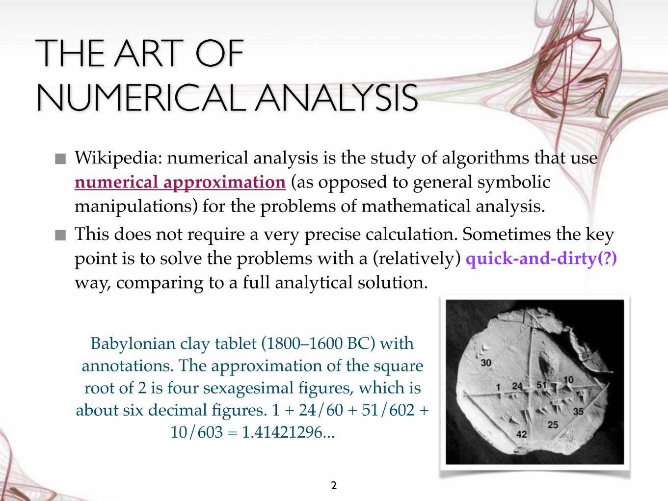
Babylonian clay tablet (1800–1600 BC) with annotations. The approximation of the square root of 2 is four sexagesimal figures, which is

about six decimal figures. 1 + 24/60 + 51/602 + 10/603 = 1.41421296...

THE ART OF NUMERICAL ANALYSIS (II)■ Thanks to the rapid development of computers, now we don’t

need to do the calculations on a piece of clay, nor with papers and pens.

■ The real speciality of computers is repetition. Your computer can do whatever any extremely boring calculations for million times. Sometimes it can be a powerful tool to solve the problems which cannot be calculated with the old fashioned way.

■ Caveat: it does not mean one can always do brainless calculations (sometimes we do!). Smarter way can provide quick and precision results; stupid way will never produce what you want.

3

THE FUN

■ This course would like to introduce you the merit of numerical analysis (or some not-so-stupid methods to solve the problems).

■ As mentioned in the first lecture, the most important goal of this course is to have fun!

■ The fun: sometimes, you may find you are able to do some extremely difficult/fancy things with only little efforts!

4

I’m going to show you a demo why the numerical analysis can be entertaining!

5

Have you ever think of converting a nice piece of tune to the sheet music?

6

Surely if you are able to find a good musician, it will work in principle...

(Still a tough job!)

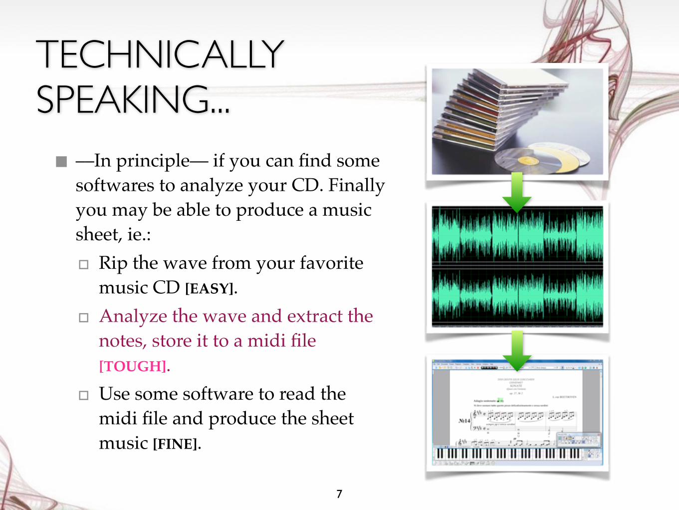
TECHNICALLY SPEAKING...■ ––In principle–– if you can find some

softwares to analyze your CD. Finally you may be able to produce a music sheet, ie.:

▫ Rip the wave from your favorite music CD [EASY].

▫ Analyze the wave and extract the notes, store it to a midi file [TOUGH].

▫ Use some software to read the midi file and produce the sheet music [FINE].

7

CATCH THE PITCH

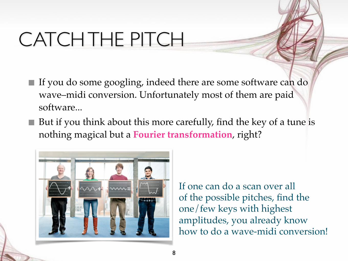
■ If you do some googling, indeed there are some software can do wave–midi conversion. Unfortunately most of them are paid software...

■ But if you think about this more carefully, find the key of a tune is nothing magical but a Fourier transformation, right?

8

If one can do a scan over all of the possible pitches, find the one/few keys with highest amplitudes, you already know how to do a wave-midi conversion!

PYTHON + SCIPY CAN DO THE WORK!■ It is not difficult at all to use Python + SciPy + NumPy to do such

a job. All you need to do are:

▫ Prepare the source wave file.

▫ Read the wave file as a NumPy array (SciPy already has such function!).

▫ For each time interval, perform the Fourier transformation (with SciPy) for each target frequency. Record the amplitudes as a function of pitch and time.

▫ Clean up (removing the noise and unwanted harmonics).

▫ Phrase the data and write to a MIDI file accordingly (with MidiUtil python package, googled).

▫ Done!

9

A CONCEPTUAL EXAMPLE

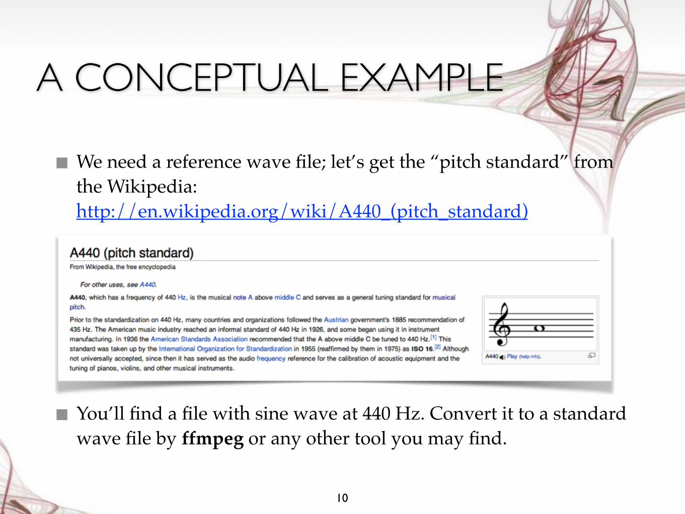
■ We need a reference wave file; let’s get the “pitch standard” from the Wikipedia: http://en.wikipedia.org/wiki/A440_(pitch_standard)

■ You’ll find a file with sine wave at 440 Hz. Convert it to a standard wave file by ffmpeg or any other tool you may find.

10

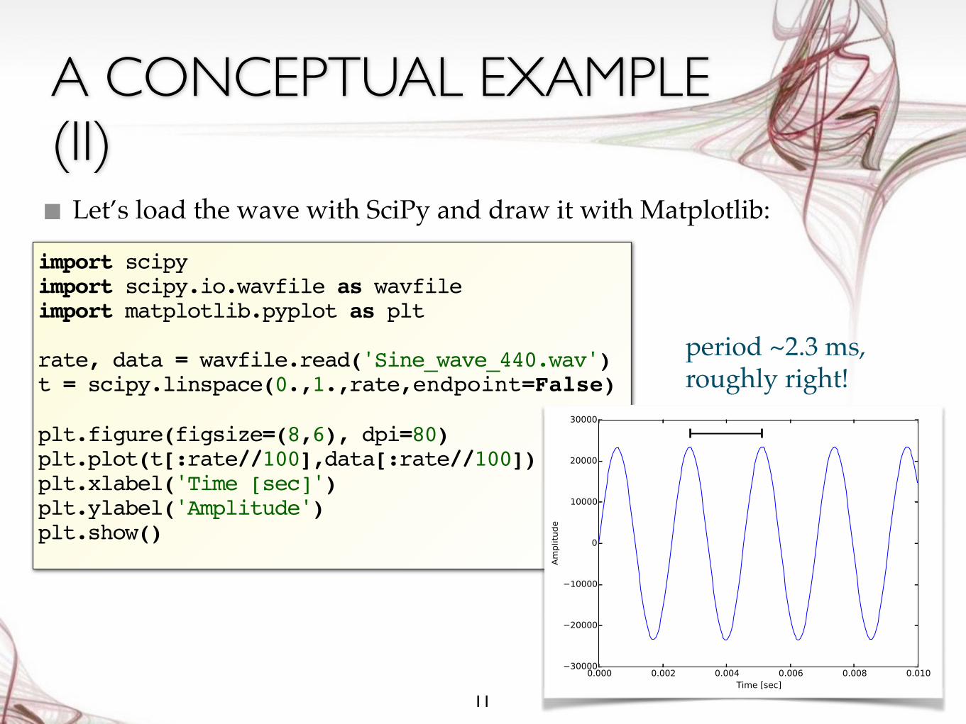
http://en.wikipedia.org/wiki/A440_(pitch_standard

A CONCEPTUAL EXAMPLE (II)■ Let’s load the wave with SciPy and draw it with Matplotlib:

11

import scipyimport scipy.io.wavfile as wavfileimport matplotlib.pyplot as plt

rate, data = wavfile.read('Sine_wave_440.wav')t = scipy.linspace(0.,1.,rate,endpoint=False)

plt.figure(figsize=(8,6), dpi=80)plt.plot(t[:rate//100],data[:rate//100])plt.xlabel('Time [sec]')plt.ylabel('Amplitude') plt.show()

period ~2.3 ms, roughly right!

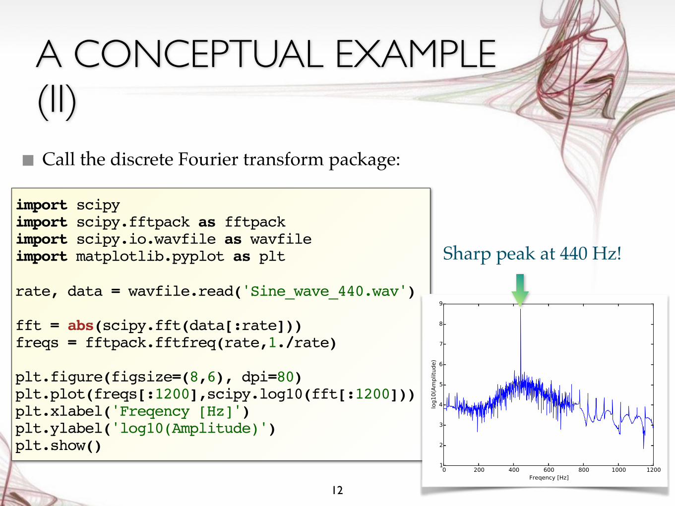
A CONCEPTUAL EXAMPLE (II)■ Call the discrete Fourier transform package:

12

import scipyimport scipy.fftpack as fftpackimport scipy.io.wavfile as wavfileimport matplotlib.pyplot as plt

rate, data = wavfile.read('Sine_wave_440.wav')

fft = abs(scipy.fft(data[:rate]))freqs = fftpack.fftfreq(rate,1./rate)

plt.figure(figsize=(8,6), dpi=80)plt.plot(freqs[:1200],scipy.log10(fft[:1200]))plt.xlabel('Freqency [Hz]')plt.ylabel('log10(Amplitude)') plt.show()

Sharp peak at 440 Hz!

STEP 1: LOADING THE WAVE

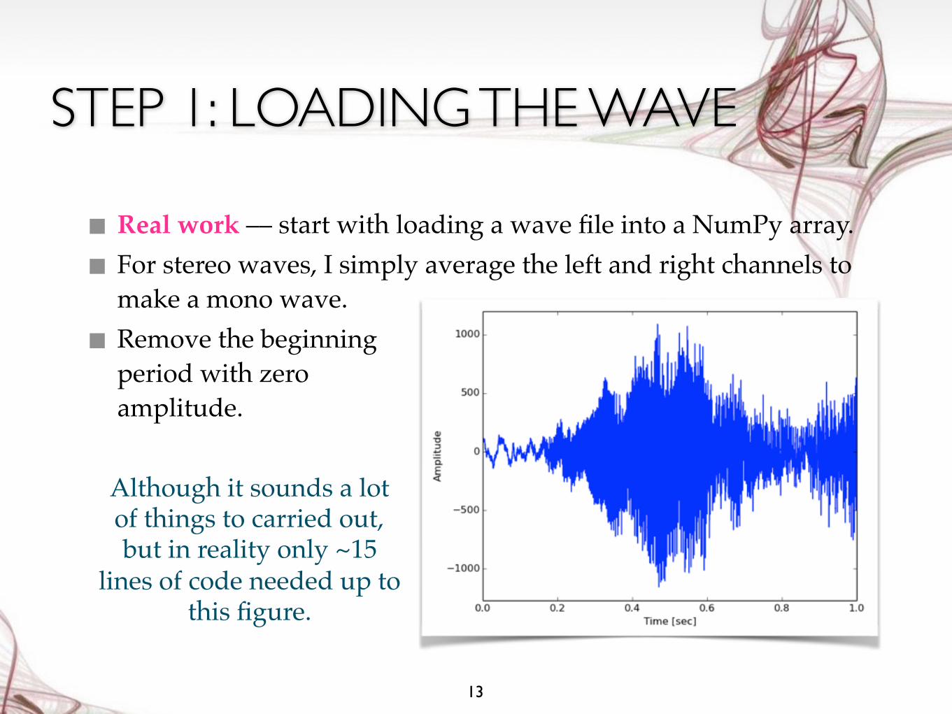
■ Real work –– start with loading a wave file into a NumPy array.

■ For stereo waves, I simply average the left and right channels to make a mono wave.

■ Remove the beginning period with zero amplitude.

13

Although it sounds a lot of things to carried out, but in reality only ~15

lines of code needed up to this figure.

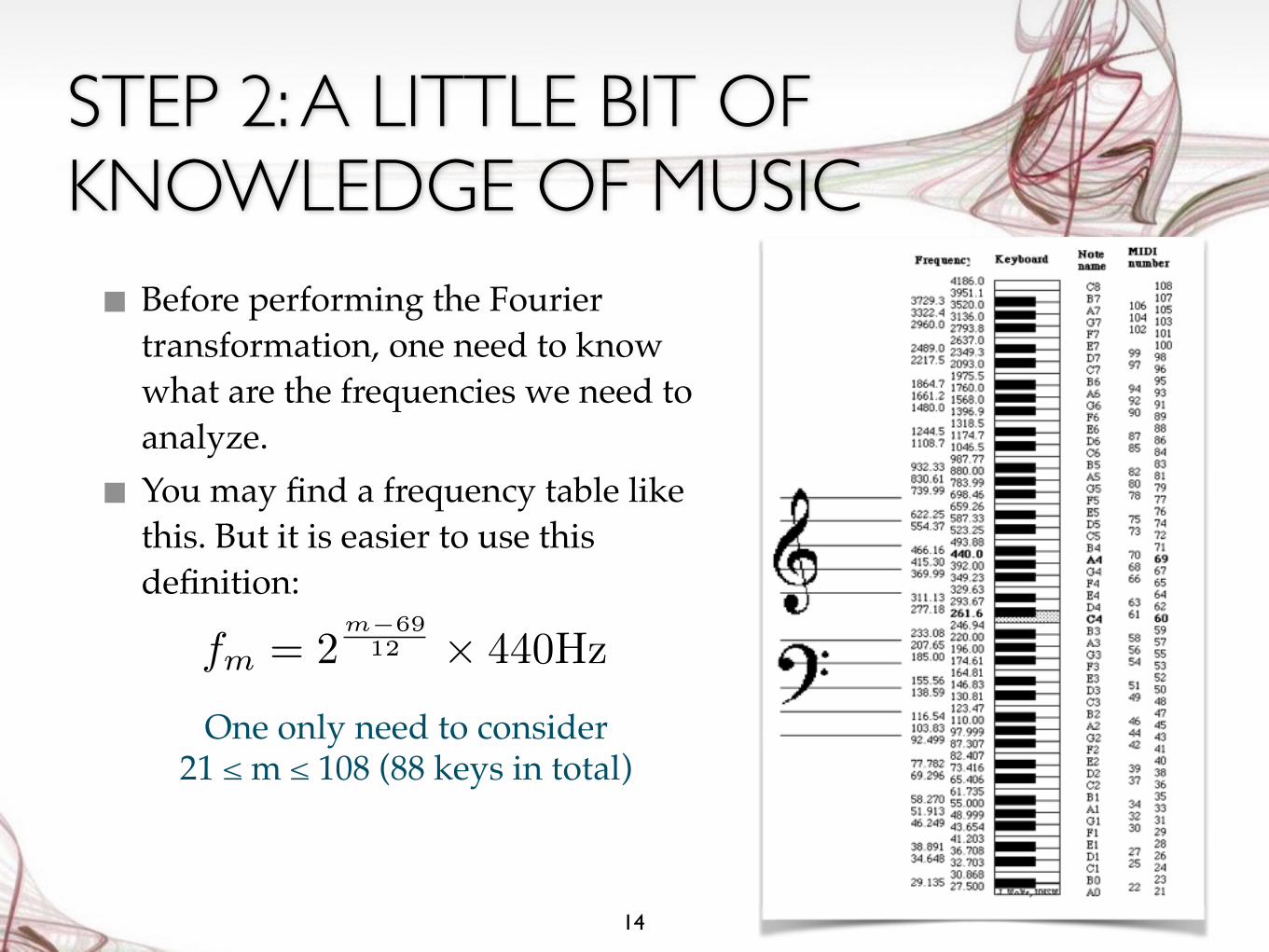
STEP 2: A LITTLE BIT OF KNOWLEDGE OF MUSIC■ Before performing the Fourier

transformation, one need to know what are the frequencies we need to analyze.

■ You may find a frequency table like this. But it is easier to use this definition:

14

fm = 2m�69

12 ⇥ 440Hz

One only need to consider 21 ≤ m ≤ 108 (88 keys in total)

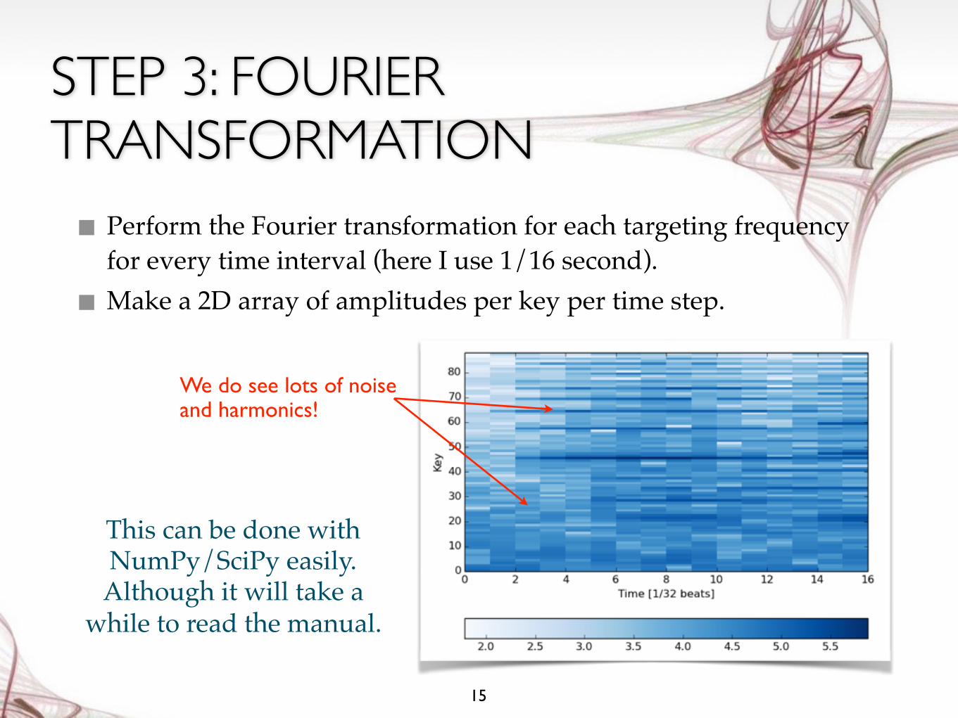
STEP 3: FOURIER TRANSFORMATION■ Perform the Fourier transformation for each targeting frequency

for every time interval (here I use 1/16 second).

■ Make a 2D array of amplitudes per key per time step.

15

This can be done with NumPy/SciPy easily. Although it will take a

while to read the manual.

We do see lots of noise and harmonics!

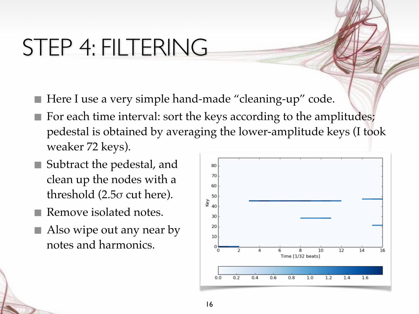
STEP 4: FILTERING

■ Here I use a very simple hand-made “cleaning-up” code.

■ For each time interval: sort the keys according to the amplitudes; pedestal is obtained by averaging the lower-amplitude keys (I took weaker 72 keys).

■ Subtract the pedestal, and clean up the nodes with a threshold (2.5σ cut here).

■ Remove isolated notes.

■ Also wipe out any near by notes and harmonics.

16

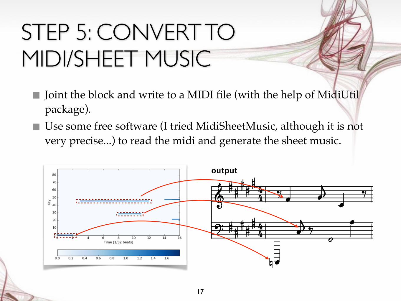
STEP 5: CONVERT TO MIDI/SHEET MUSIC■ Joint the block and write to a MIDI file (with the help of MidiUtil

package).

■ Use some free software (I tried MidiSheetMusic, although it is not very precise...) to read the midi and generate the sheet music.

17

1

output

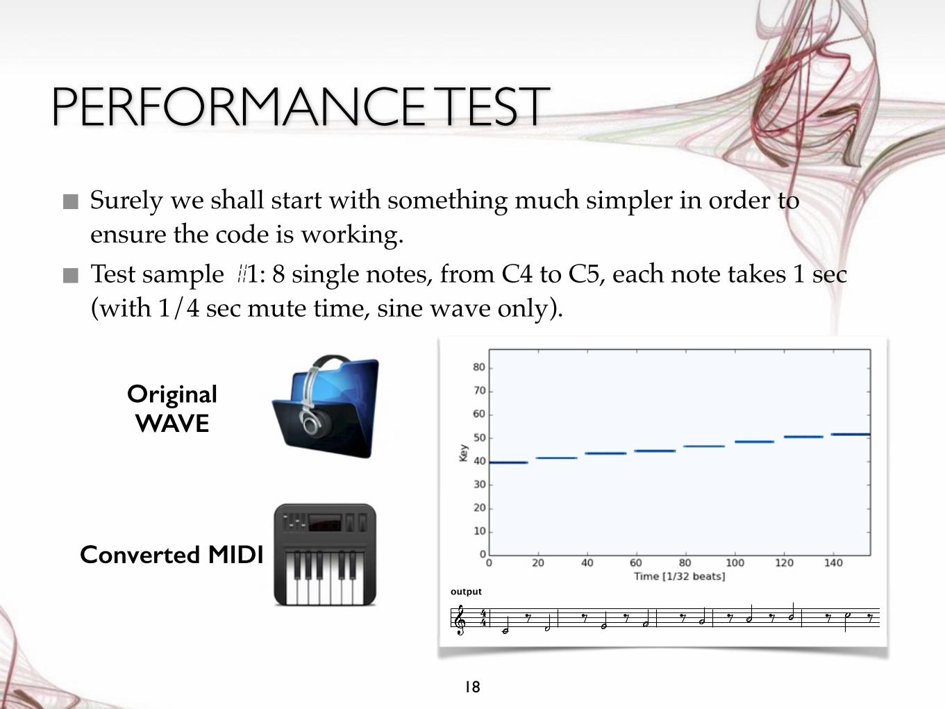
PERFORMANCE TEST■ Surely we shall start with something much simpler in order to

ensure the code is working.

■ Test sample #1: 8 single notes, from C4 to C5, each note takes 1 sec (with 1/4 sec mute time, sine wave only).

18

1

output

Original WAVE

Converted MIDI

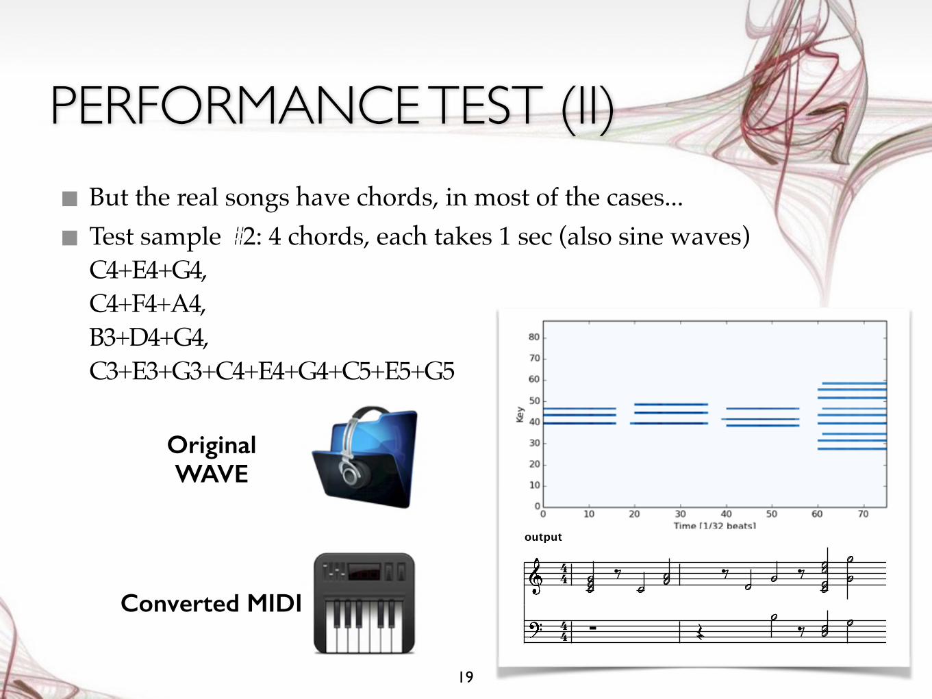
■ But the real songs have chords, in most of the cases...

■ Test sample #2: 4 chords, each takes 1 sec (also sine waves) C4+E4+G4,C4+F4+A4,B3+D4+G4,C3+E3+G3+C4+E4+G4+C5+E5+G5

PERFORMANCE TEST (II)

19

1

output

Original WAVE

Converted MIDI

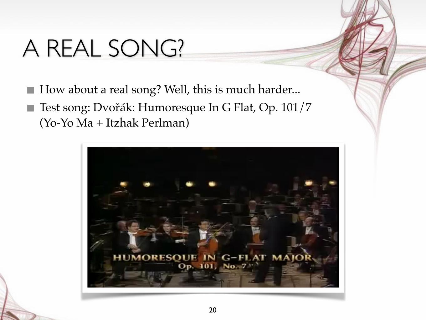
A REAL SONG?■ How about a real song? Well, this is much harder...

■ Test song: Dvořák: Humoresque In G Flat, Op. 101/7 (Yo-Yo Ma + Itzhak Perlman)

20

1

output

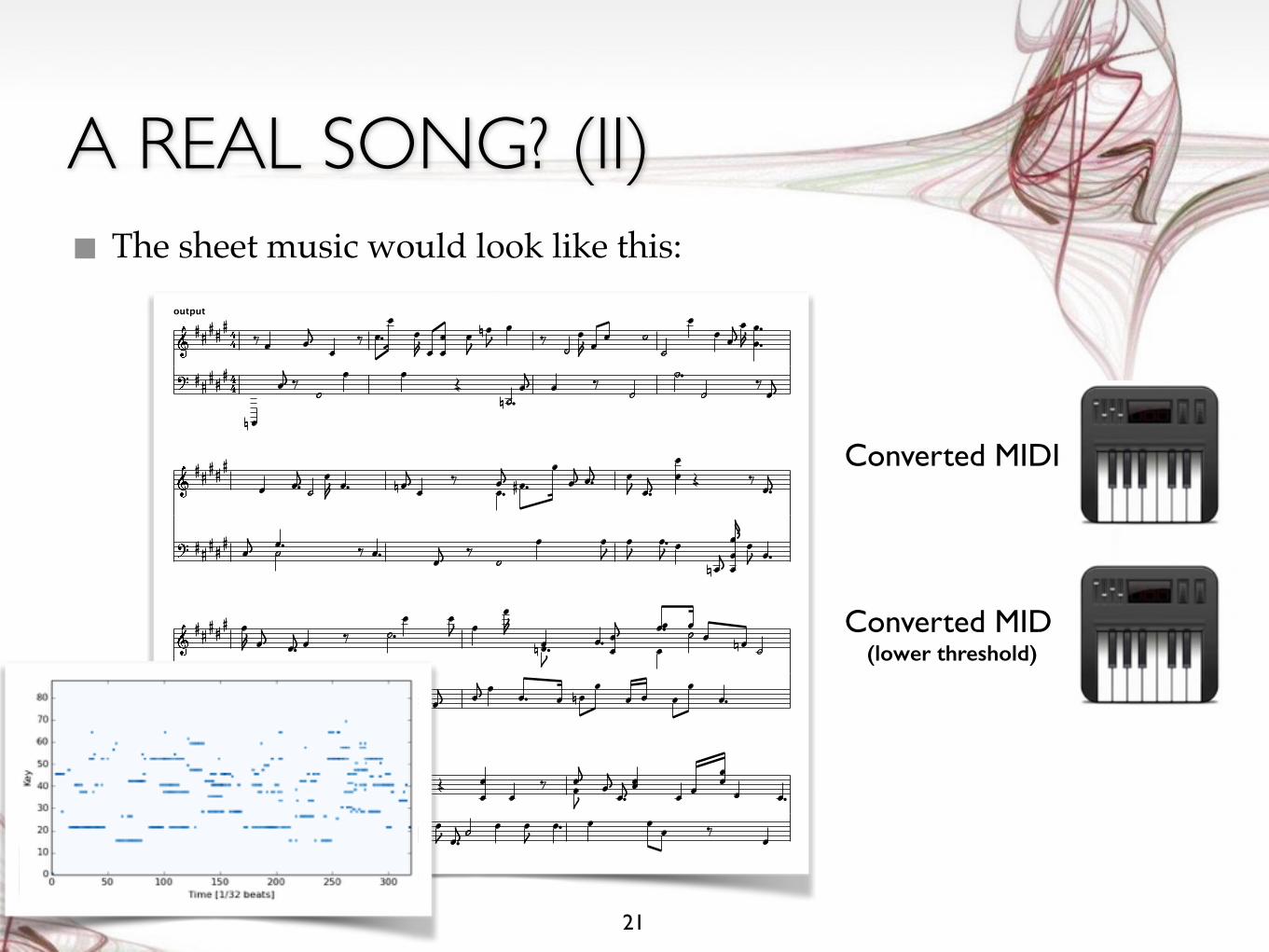
A REAL SONG? (II)■ The sheet music would look like this:

21

Converted MIDI

Converted MIDI(lower threshold)

COMMENTS

■ You probably noticed this is not trivial to analyze a real song with such a super naive code (but it is already fancy enough, right?)

■ With some more googling, it seems that doing such thing (analyzing a wave and catching the right pitch) is a research level (still in development) topic.

■ With the support of NumPy and SciPy, doing all the work above only requires ~200 lines of coding. It is not difficult at all –– surely it will not be easy if you want to improve the performance further.

22

All the work done here is already a nice demo of numerical analysis (and it is FUN!).

INTERMISSION

■ Anybody wants to sing a song and let’s convert it to a MIDI file?

23

Then we will come back with the first step toward numerical analysis –– errors in computation.

FIRST STEP TOWARD NUMERICAL ANALYSIS: ERRORS IN COMPUTATION

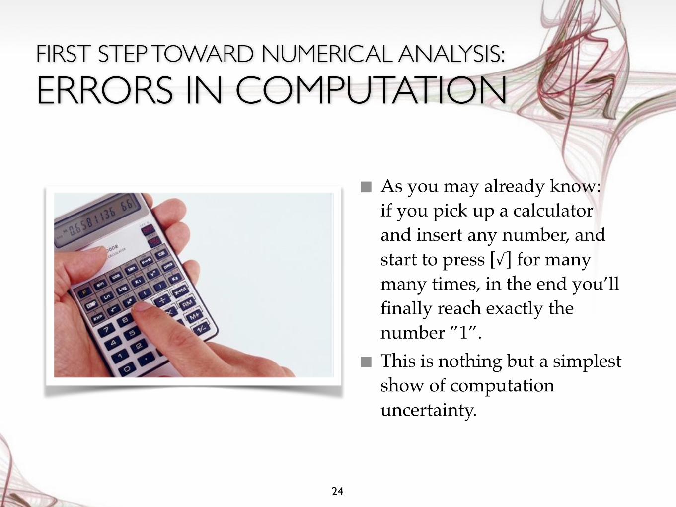
■ As you may already know: if you pick up a calculator and insert any number, and start to press [√] for many many times, in the end you’ll finally reach exactly the number ”1”.

■ This is nothing but a simplest show of computation uncertainty.

24

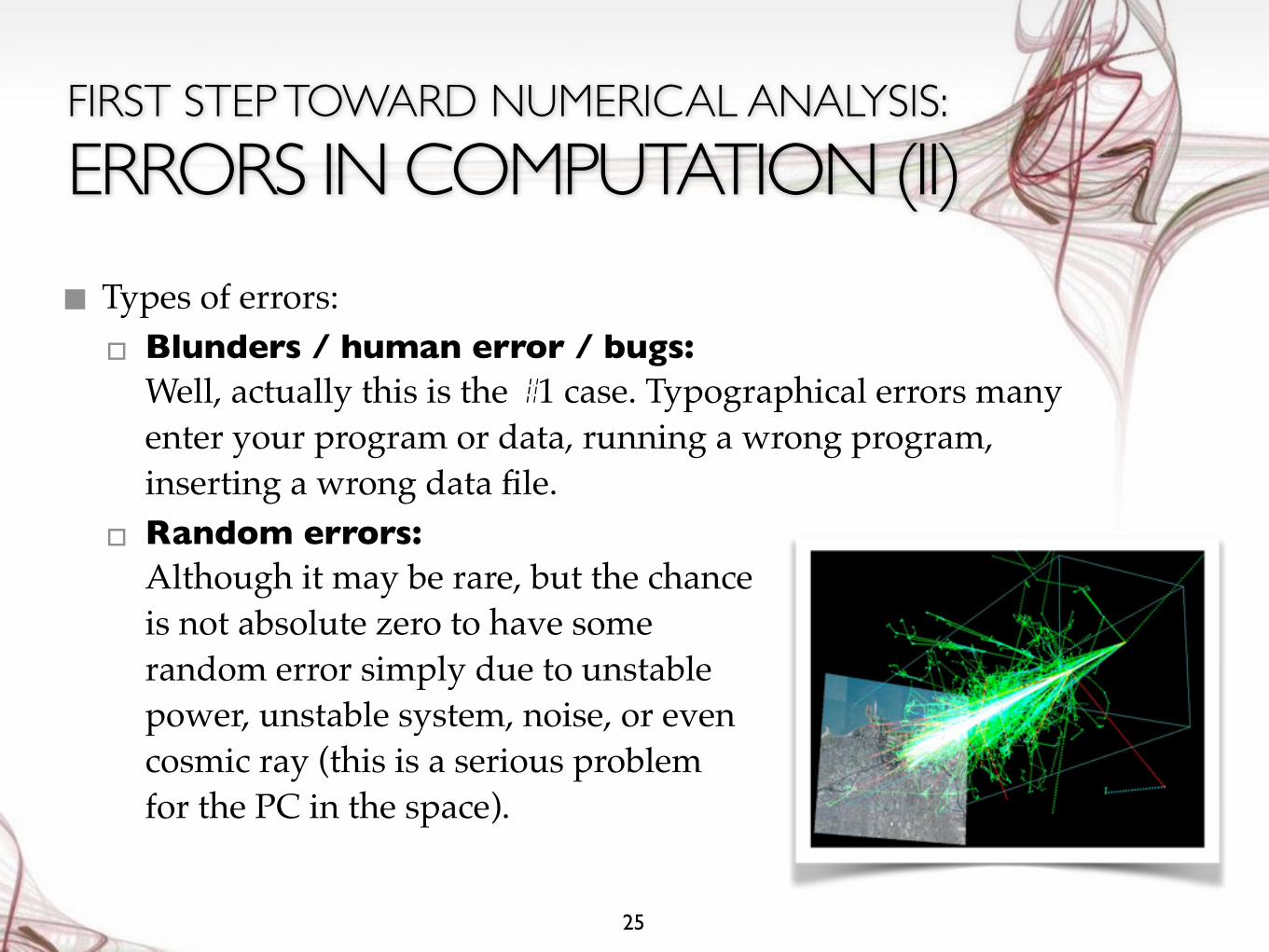
FIRST STEP TOWARD NUMERICAL ANALYSIS: ERRORS IN COMPUTATION (II)■ Types of errors:▫ Blunders / human error / bugs:

Well, actually this is the #1 case. Typographical errors many enter your program or data, running a wrong program, inserting a wrong data file.▫ Random errors:

Although it may be rare, but the chance is not absolute zero to have some random error simply due to unstable power, unstable system, noise, or even cosmic ray (this is a serious problem for the PC in the space).

25

FIRST STEP TOWARD NUMERICAL ANALYSIS: ERRORS IN COMPUTATION (III)■ Types of errors (cont.):▫ Approximation errors:

Basically, this is the error due to the selected algorithm. In principle if we throw away some higher order term, naturally we have this error in the calculations.▫ Roundoff errors:

Surely, the numbers (especially the float point numbers) in the computers are not infinitely precise. Then it's very easy to have this round-off error at the end of the digits.

26

Today we will discuss these two types of errors.Assuming I made no mistake and the cosmic muons

do not hit my PC.

BITS, BYTES, INTEGERS...

■ A bit is the basic unit in computing and physically implemented with a two-state device (0 or 1).

■ Historically, the byte was the number of bits used to encode a single character. Now it has been fixed to 8 bits, permitting the values between 0 and 255 (=28-1).

■ In python, the integer are implemented using long in C, which gives them 8 bytes (64 bits) of precision. The long integers in python have unlimited precision.

27

Range of integer: –(263) ~ (263)–1The long type in python can be very long, e.g.

123456789123456789123456789123456789123456789In python 2, the long integers and integers are different (need to add“L” in the end for python 2).

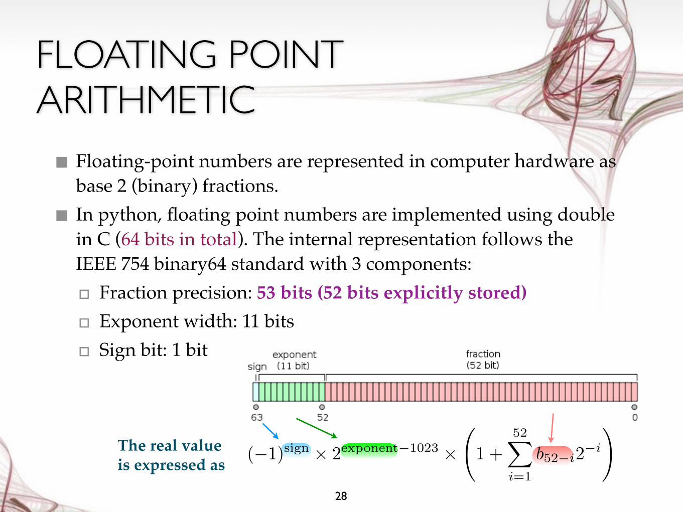
FLOATING POINT ARITHMETIC■ Floating-point numbers are represented in computer hardware as

base 2 (binary) fractions.

■ In python, floating point numbers are implemented using double in C (64 bits in total). The internal representation follows the IEEE 754 binary64 standard with 3 components:

▫ Fraction precision: 53 bits (52 bits explicitly stored)

▫ Exponent width: 11 bits

▫ Sign bit: 1 bit

28

(�1)sign ⇥ 2exponent�1023 ⇥ 1 +

52X

i=1

b52�i2

�i

!The real value is expressed as

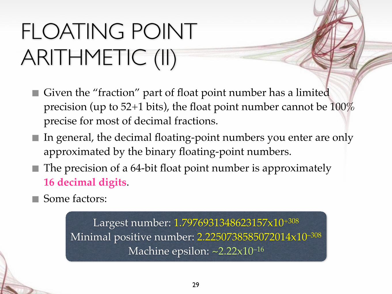
FLOATING POINT ARITHMETIC (II)■ Given the “fraction” part of float point number has a limited

precision (up to 52+1 bits), the float point number cannot be 100% precise for most of decimal fractions.

■ In general, the decimal floating-point numbers you enter are only approximated by the binary floating-point numbers.

■ The precision of a 64-bit float point number is approximately 16 decimal digits.

■ Some factors:

29

Largest number: 1.7976931348623157x10+308

Minimal positive number: 2.2250738585072014x10–308

Machine epsilon: ~2.22x10–16

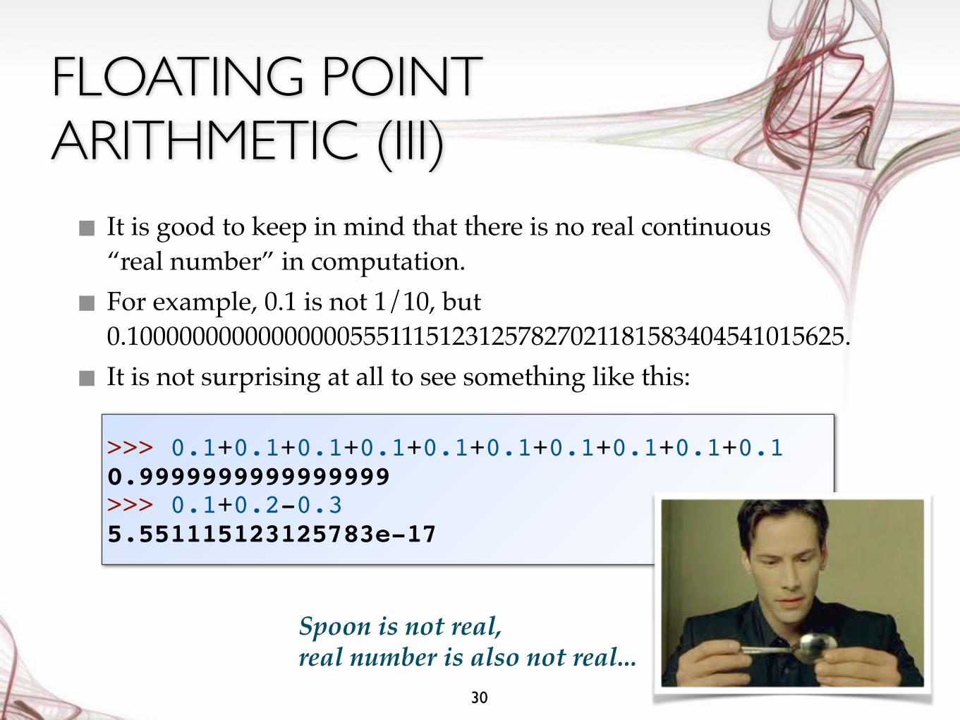
FLOATING POINT ARITHMETIC (III)■ It is good to keep in mind that there is no real continuous

“real number” in computation.

■ For example, 0.1 is not 1/10, but 0.1000000000000000055511151231257827021181583404541015625.

■ It is not surprising at all to see something like this:

30

>>> 0.1+0.1+0.1+0.1+0.1+0.1+0.1+0.1+0.1+0.10.9999999999999999 >>> 0.1+0.2-0.35.551115123125783e-17

Spoon is not real, real number is also not real...

31

Let’s take the standard example of π calculation!

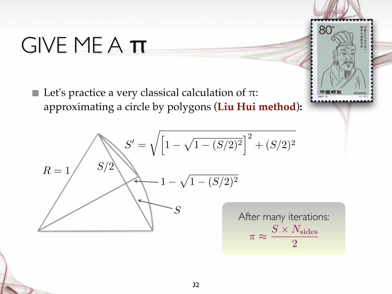
GIVE ME A π

■ Let's practice a very classical calculation of π: approximating a circle by polygons (Liu Hui method):

32

After many iterations:

S0 =

rh1�

p1� (S/2)2

i2+ (S/2)2

1�p

1� (S/2)2S/2R = 1

S

⇡ ⇡ S ⇥Nsides

2

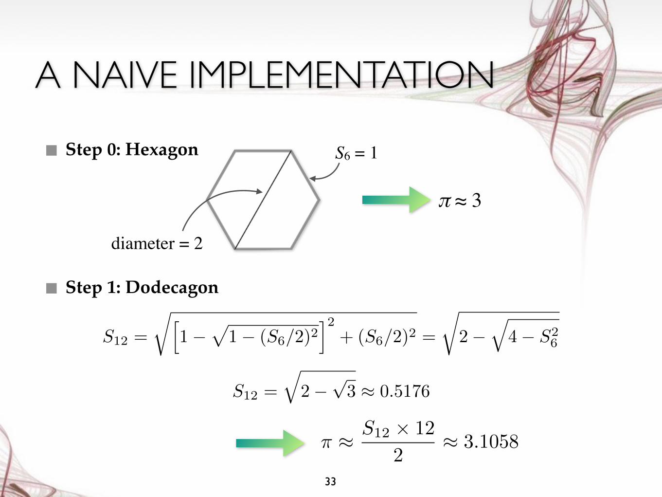
A NAIVE IMPLEMENTATION

33

■ Step 0: Hexagon

■ Step 1: Dodecagon

diameter = 2

S6 = 1

π ≈ 3

S12 =

rh1�

p1� (S6/2)2

i2+ (S6/2)2 =

r2�

q4� S2

6

S12 =

q2�

p3 ⇡ 0.5176

⇡ ⇡ S12 ⇥ 12

2⇡ 3.1058

A NAIVE IMPLEMENTATION (II)

34

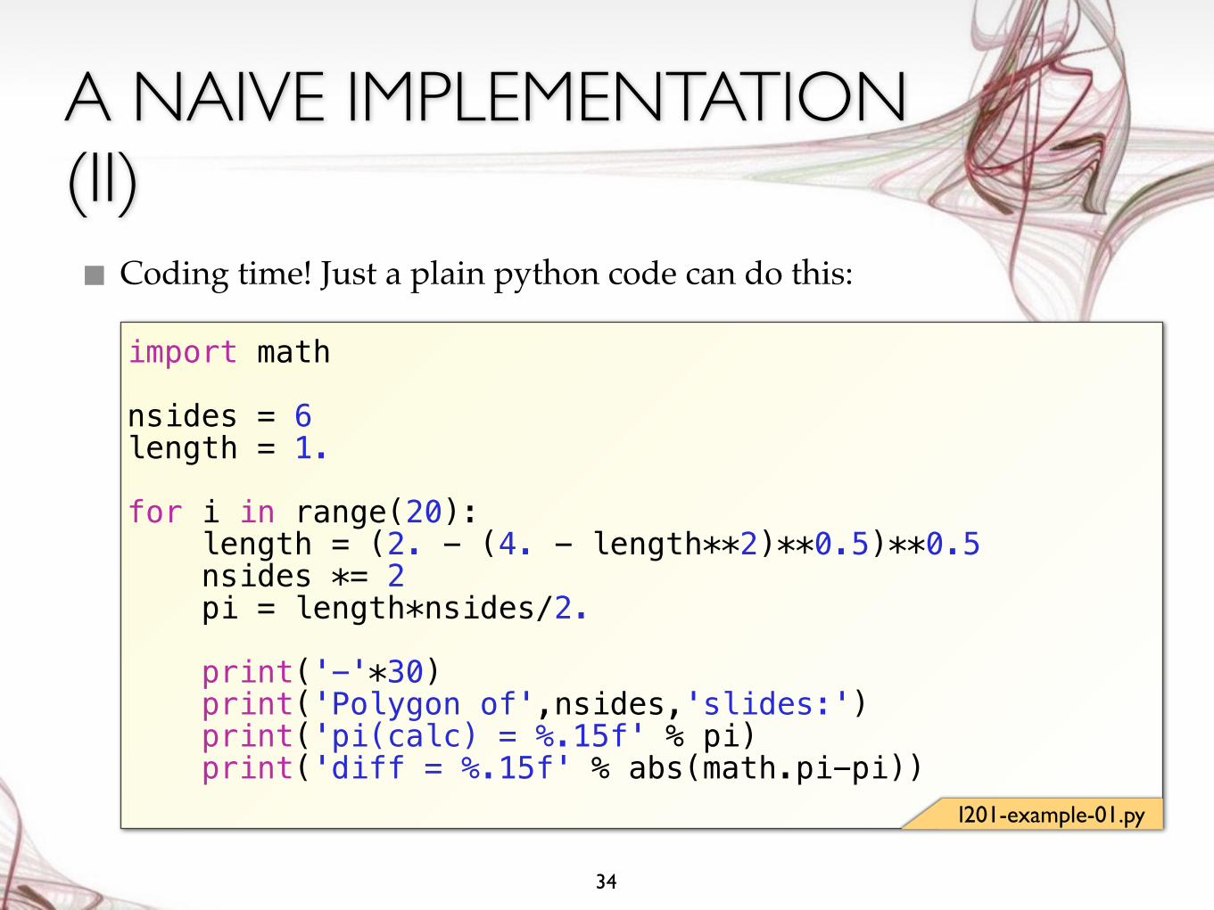
■ Coding time! Just a plain python code can do this:

import math

nsides = 6 length = 1.

for i in range(20): length = (2. - (4. - length**2)**0.5)**0.5 nsides *= 2 pi = length*nsides/2.

print('-'*30) print('Polygon of',nsides,'slides:') print('pi(calc) = %.15f' % pi) print('diff = %.15f' % abs(math.pi-pi))

l201-example-01.py

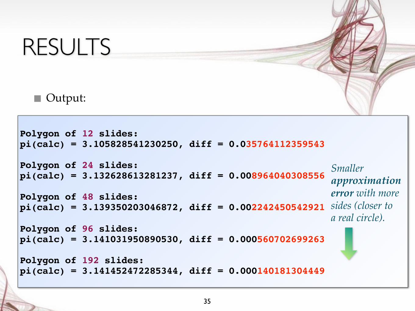
RESULTS

■ Output:

35

Polygon of 12 slides:pi(calc) = 3.105828541230250, diff = 0.035764112359543





Smaller approximationerror with more sides (closer to a real circle).

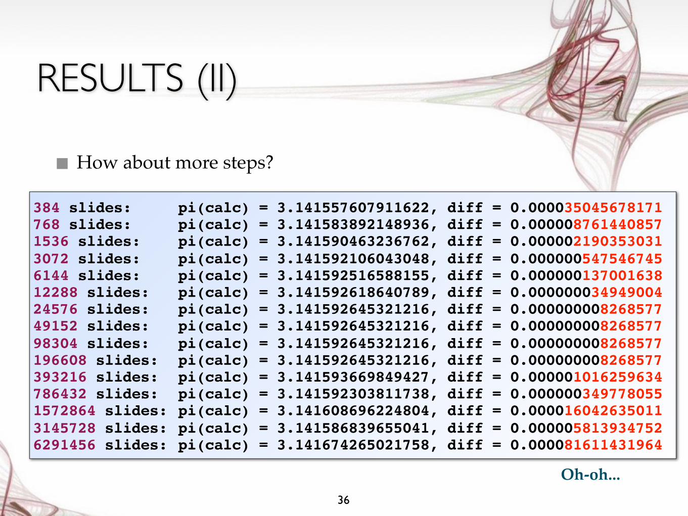
RESULTS (II)

■ How about more steps?

36

384 slides: pi(calc) = 3.141557607911622, diff = 0.000035045678171768 slides: pi(calc) = 3.141583892148936, diff = 0.0000087614408571536 slides: pi(calc) = 3.141590463236762, diff = 0.0000021903530313072 slides: pi(calc) = 3.141592106043048, diff = 0.0000005475467456144 slides: pi(calc) = 3.141592516588155, diff = 0.00000013700163812288 slides: pi(calc) = 3.141592618640789, diff = 0.00000003494900424576 slides: pi(calc) = 3.141592645321216, diff = 0.00000000826857749152 slides: pi(calc) = 3.141592645321216, diff = 0.00000000826857798304 slides: pi(calc) = 3.141592645321216, diff = 0.000000008268577196608 slides: pi(calc) = 3.141592645321216, diff = 0.000000008268577393216 slides: pi(calc) = 3.141593669849427, diff = 0.000001016259634786432 slides: pi(calc) = 3.141592303811738, diff = 0.0000003497780551572864 slides: pi(calc) = 3.141608696224804, diff = 0.0000160426350113145728 slides: pi(calc) = 3.141586839655041, diff = 0.0000058139347526291456 slides: pi(calc) = 3.141674265021758, diff = 0.000081611431964

Oh-oh...

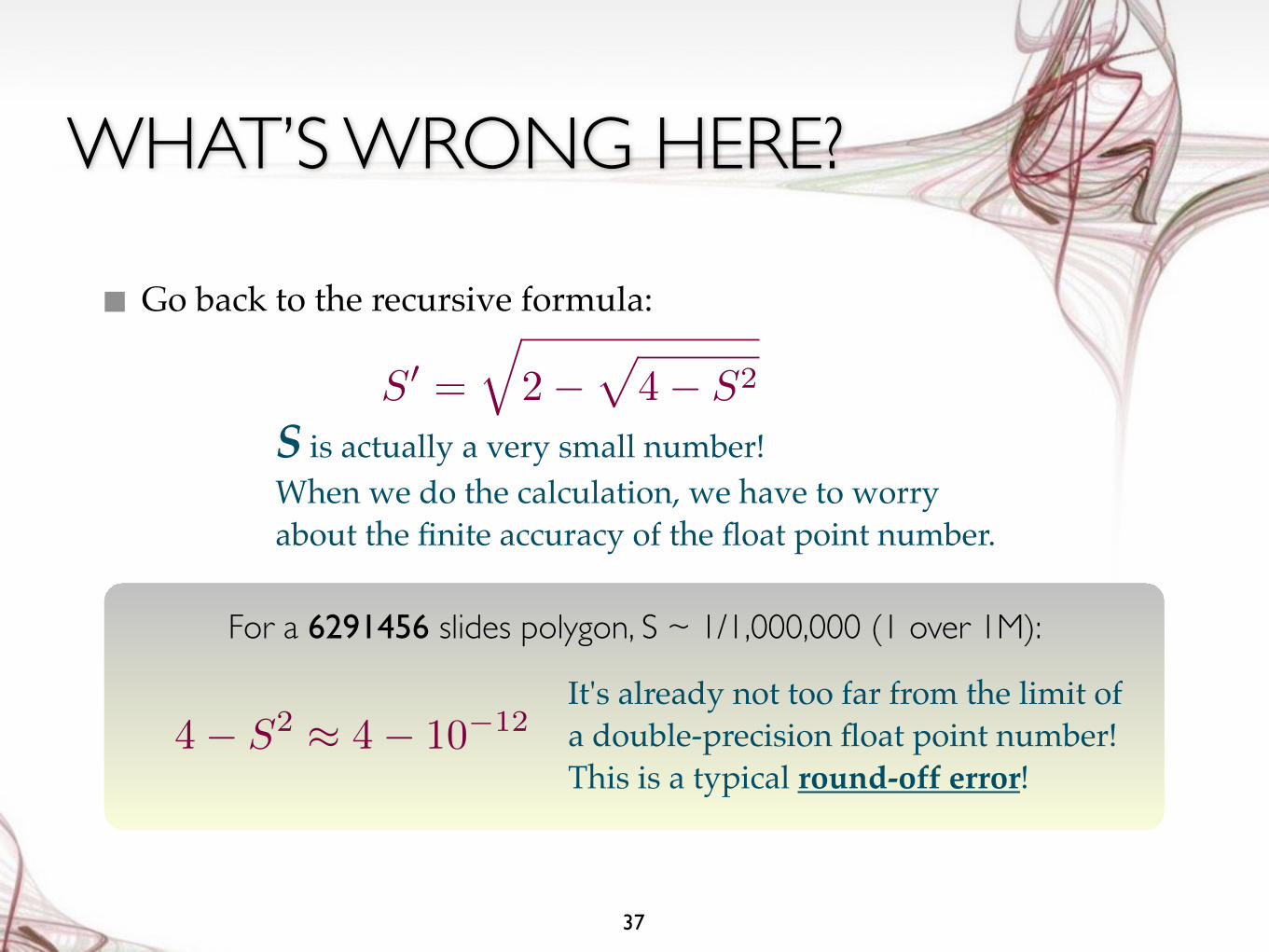
WHAT’S WRONG HERE?

■ Go back to the recursive formula:

37

S0 =

q2�

p4� S2

S is actually a very small number!When we do the calculation, we have to worry about the finite accuracy of the float point number.

For a 6291456 slides polygon, S ~ 1/1,000,000 (1 over 1M):

It's already not too far from the limit of a double-precision float point number!This is a typical round-off error!

4� S2 ⇡ 4� 10�12

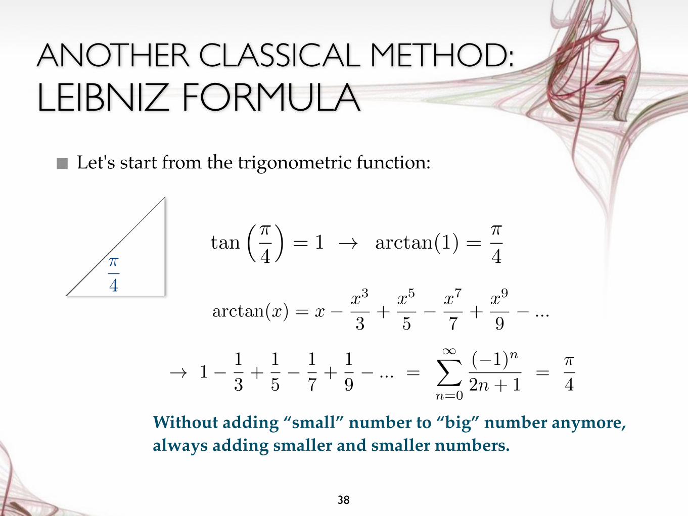
ANOTHER CLASSICAL METHOD:LEIBNIZ FORMULA■ Let's start from the trigonometric function:

38

Without adding “small” number to “big” number anymore, always adding smaller and smaller numbers.

tan⇣⇡4

⌘= 1 ! arctan(1) =

⇡

4

arctan(x) = x� x

3

3+

x

5

5� x

7

7+

x

9

9� ...

! 1� 1

3+

1

5� 1

7+

1

9� ... =

1X

n=0

(�1)n

2n+ 1=

⇡

4

⇡

4

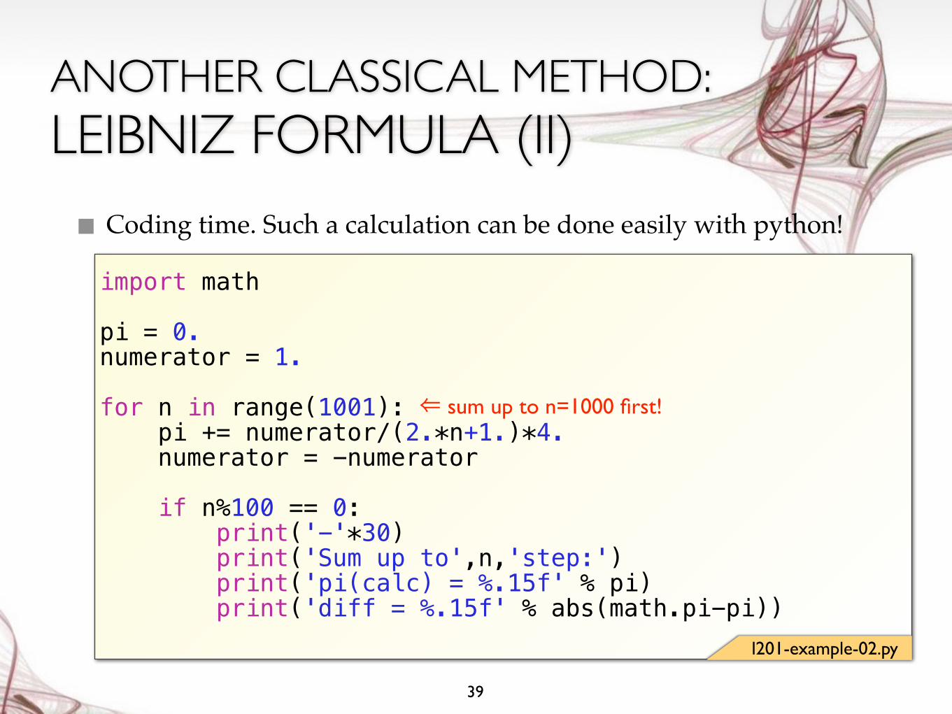
ANOTHER CLASSICAL METHOD:LEIBNIZ FORMULA (II)■ Coding time. Such a calculation can be done easily with python!

39

import math

pi = 0. numerator = 1.

for n in range(1001): pi += numerator/(2.*n+1.)*4. numerator = -numerator if n%100 == 0: print('-'*30) print('Sum up to',n,'step:') print('pi(calc) = %.15f' % pi) print('diff = %.15f' % abs(math.pi-pi))

l201-example-02.py

⇐ sum up to n=1000 first!

RESULTS: LIEBNIZ FORMULA

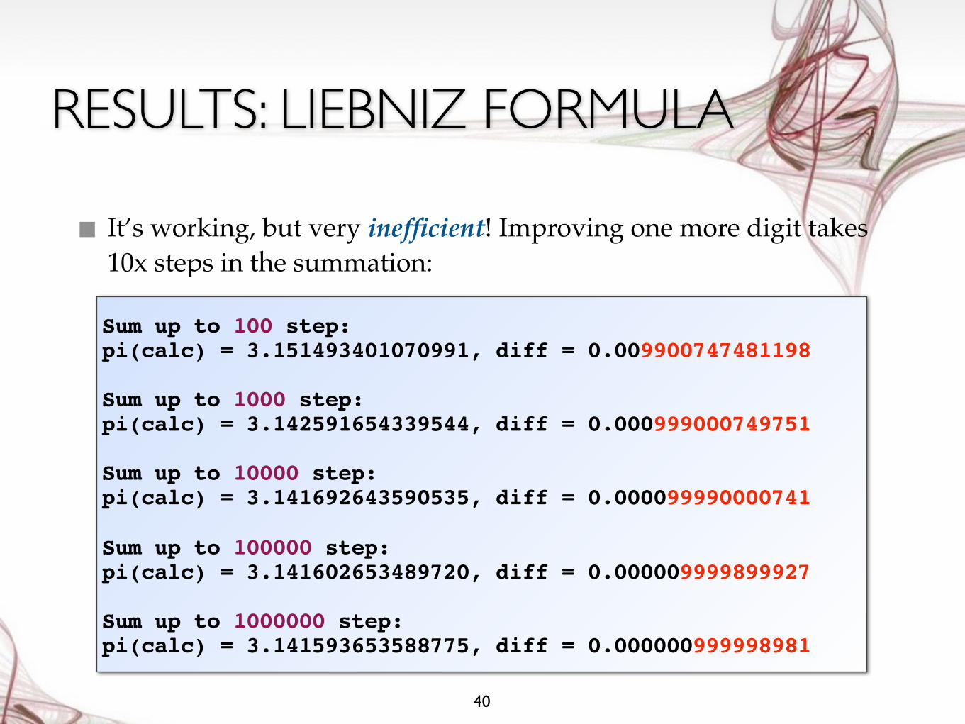
■ It’s working, but very inefficient! Improving one more digit takes 10x steps in the summation:

40

Sum up to 100 step:pi(calc) = 3.151493401070991, diff = 0.009900747481198





A LITTLE BIT OF IMPROVEMENT (A TRICK!)■ It's not really hard: we can just pick up a smaller x!

41

arctan(x) = x� x

3

3+

x

5

5� x

7

7+

x

9

9� ...

⇡

6

1

p3

tan⇣⇡6

⌘=

1p3

! arctan

✓1p3

◆=

⇡

6

! 1p3[1� 1

3 · 3 +1

5 · 9 � 1

7 · 27 +1

9 · 81 � ...] =⇡

6

It converges much quicker then the previous version. This is due to that the Taylor expansions are calculated around x = 0.

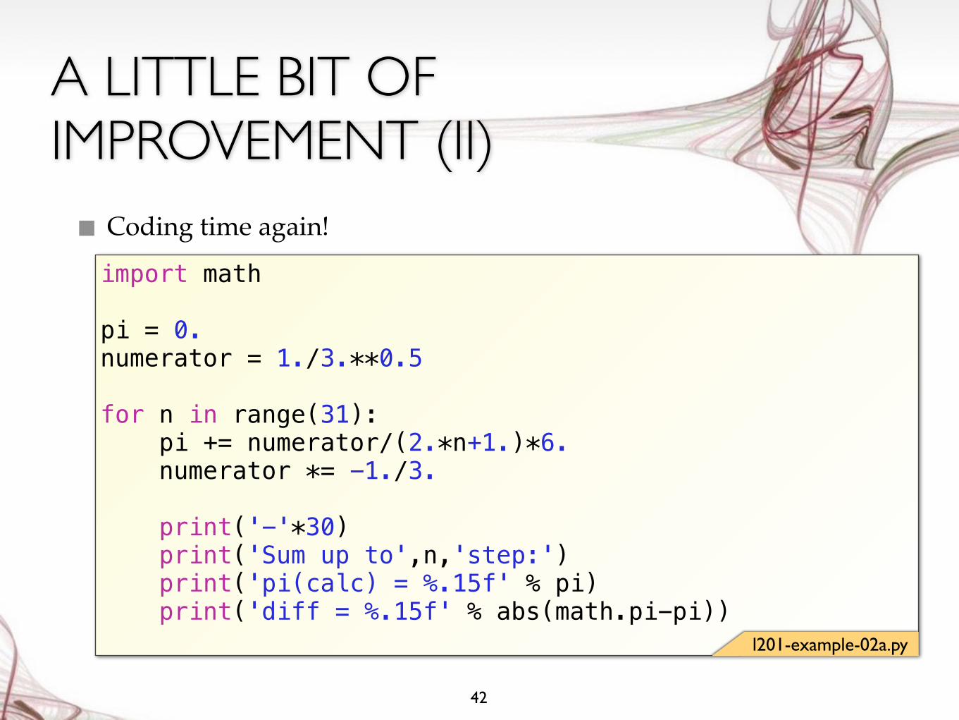
A LITTLE BIT OF IMPROVEMENT (II)■ Coding time again!

42

import math

pi = 0. numerator = 1./3.**0.5

for n in range(31): pi += numerator/(2.*n+1.)*6. numerator *= -1./3. print('-'*30) print('Sum up to',n,'step:') print('pi(calc) = %.15f' % pi) print('diff = %.15f' % abs(math.pi-pi))

l201-example-02a.py

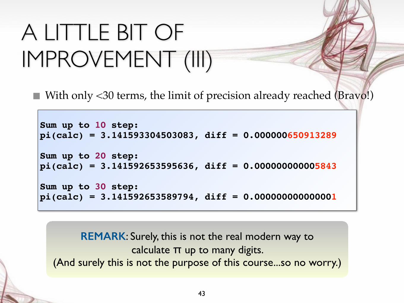
A LITTLE BIT OF IMPROVEMENT (III)■ With only <30 terms, the limit of precision already reached (Bravo!)

43




REMARK: Surely, this is not the real modern way to calculate π up to many digits.

(And surely this is not the purpose of this course...so no worry.)

44

Calculation of π is in fact rather interesting. Left for

your own study!

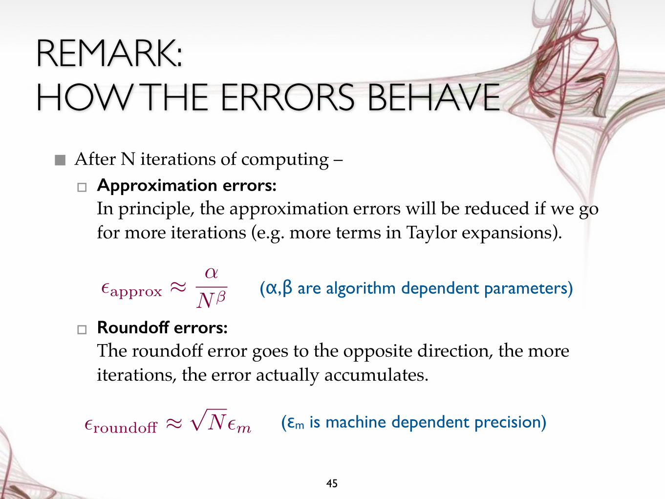
REMARK: HOW THE ERRORS BEHAVE■ After N iterations of computing –▫ Approximation errors:

In principle, the approximation errors will be reduced if we go for more iterations (e.g. more terms in Taylor expansions).

▫ Roundoff errors: The roundoff error goes to the opposite direction, the more iterations, the error actually accumulates.

45

✏approx

⇡ ↵

N�

✏roundo↵

⇡pN✏m

(α,β are algorithm dependent parameters)

(εm is machine dependent precision)

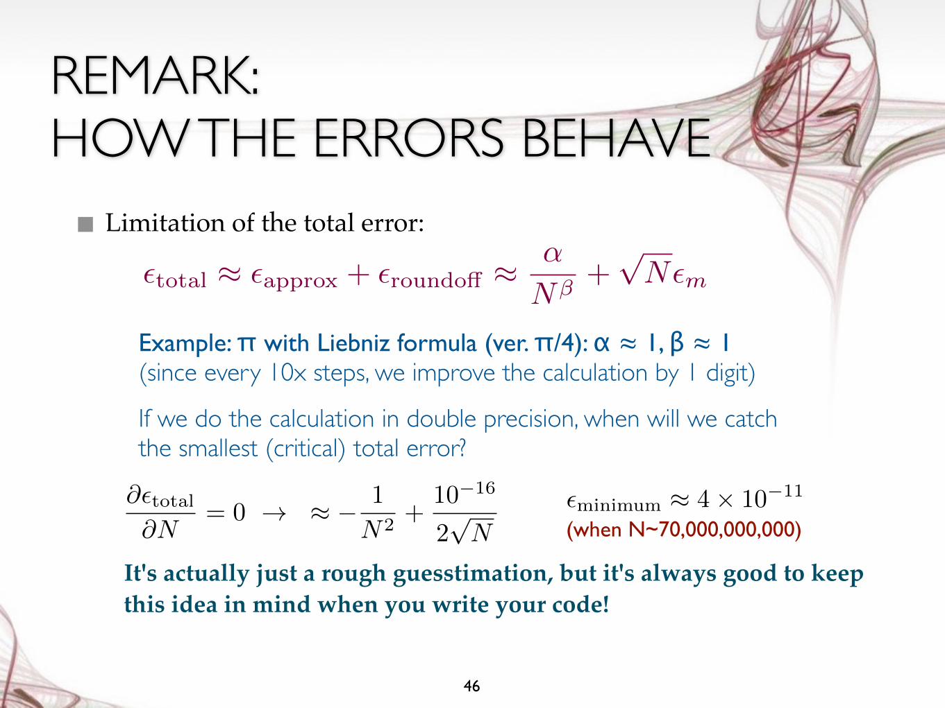
REMARK: HOW THE ERRORS BEHAVE■ Limitation of the total error:

46

Example: π with Liebniz formula (ver. π/4): α ≈ 1, β ≈ 1 (since every 10x steps, we improve the calculation by 1 digit)

If we do the calculation in double precision, when will we catchthe smallest (critical) total error?

✏total

⇡ ✏approx

+ ✏roundo↵

⇡ ↵

N�+

pN✏m

@✏total

@N= 0 ! ⇡ � 1

N2

+10�16

2pN

✏minimum ⇡ 4⇥ 10�11

(when N~70,000,000,000)

It's actually just a rough guesstimation, but it's always good to keep this idea in mind when you write your code!

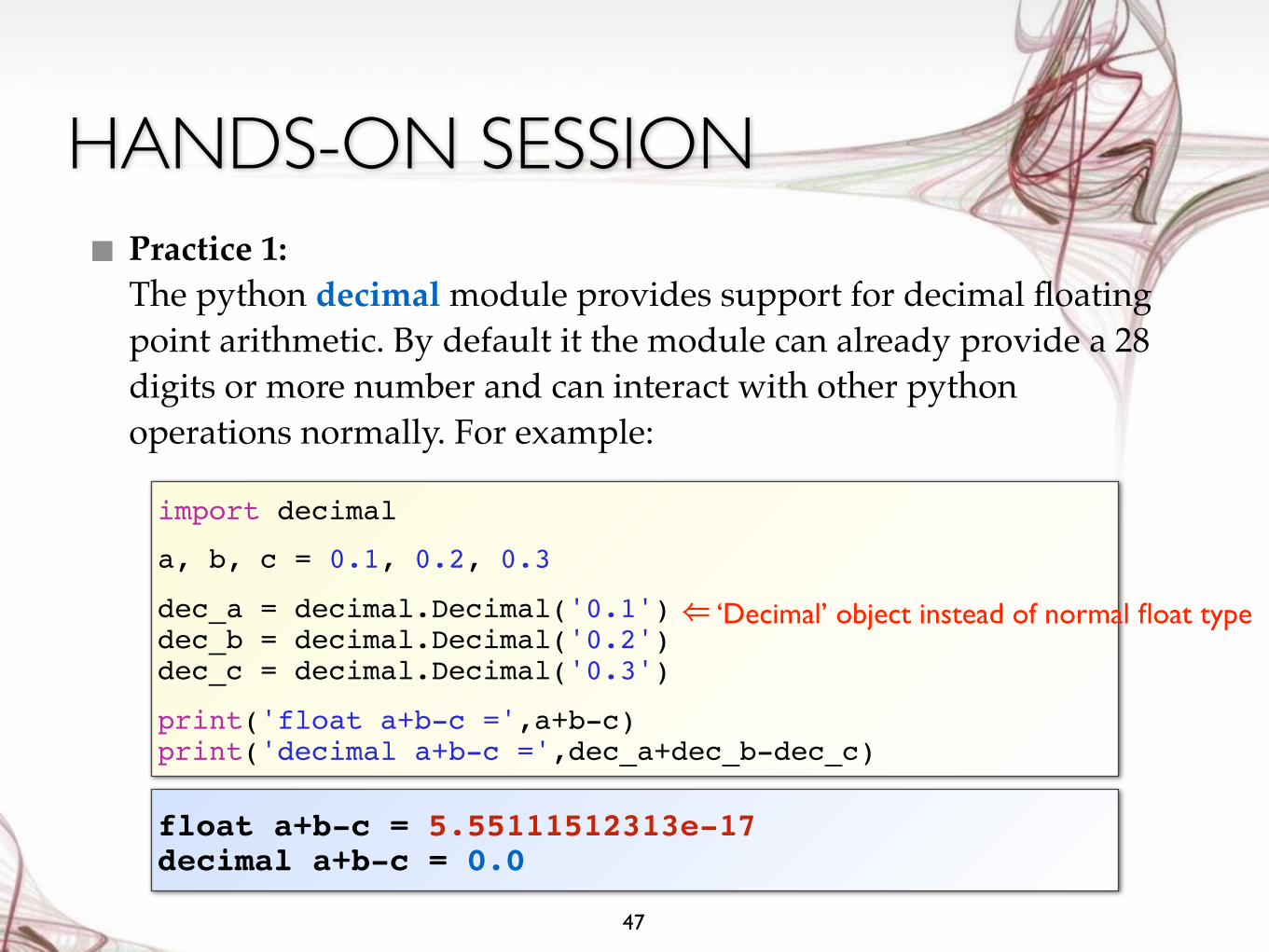
HANDS-ON SESSION■ Practice 1:

The python decimal module provides support for decimal floating point arithmetic. By default it the module can already provide a 28 digits or more number and can interact with other python operations normally. For example:

47

float a+b-c = 5.55111512313e-17decimal a+b-c = 0.0

import decimal

a, b, c = 0.1, 0.2, 0.3

dec_a = decimal.Decimal('0.1')dec_b = decimal.Decimal('0.2')dec_c = decimal.Decimal('0.3')

print('float a+b-c =',a+b-c)print('decimal a+b-c =',dec_a+dec_b-dec_c)

⇐ ‘Decimal’ object instead of normal float type

HANDS-ON SESSION

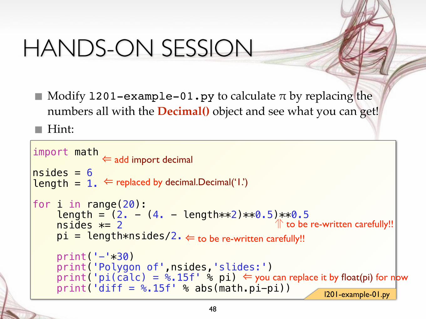
■ Modify l201-example-01.py to calculate π by replacing the numbers all with the Decimal() object and see what you can get!

■ Hint:

48

import math

nsides = 6 length = 1.

for i in range(20): length = (2. - (4. - length**2)**0.5)**0.5 nsides *= 2 pi = length*nsides/2.

print('-'*30) print('Polygon of',nsides,'slides:') print('pi(calc) = %.15f' % pi) print('diff = %.15f' % abs(math.pi-pi))

l201-example-01.py

⇐ add import decimal

⇐ replaced by decimal.Decimal(‘1.’)

⇑ to be re-written carefully!!

⇐ to be re-written carefully!!

⇐ you can replace it by float(pi) for now

HANDS-ON SESSION

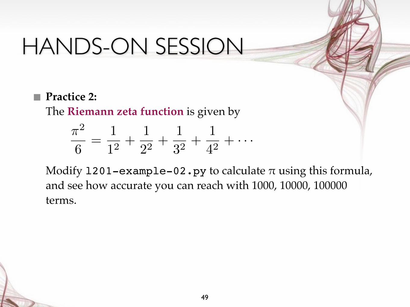
■ Practice 2: The Riemann zeta function is given by Modify l201-example-02.py to calculate π using this formula, and see how accurate you can reach with 1000, 10000, 100000 terms.

49

⇡2

6=

1

12+

1

22+

1

32+

1

42+ · · ·

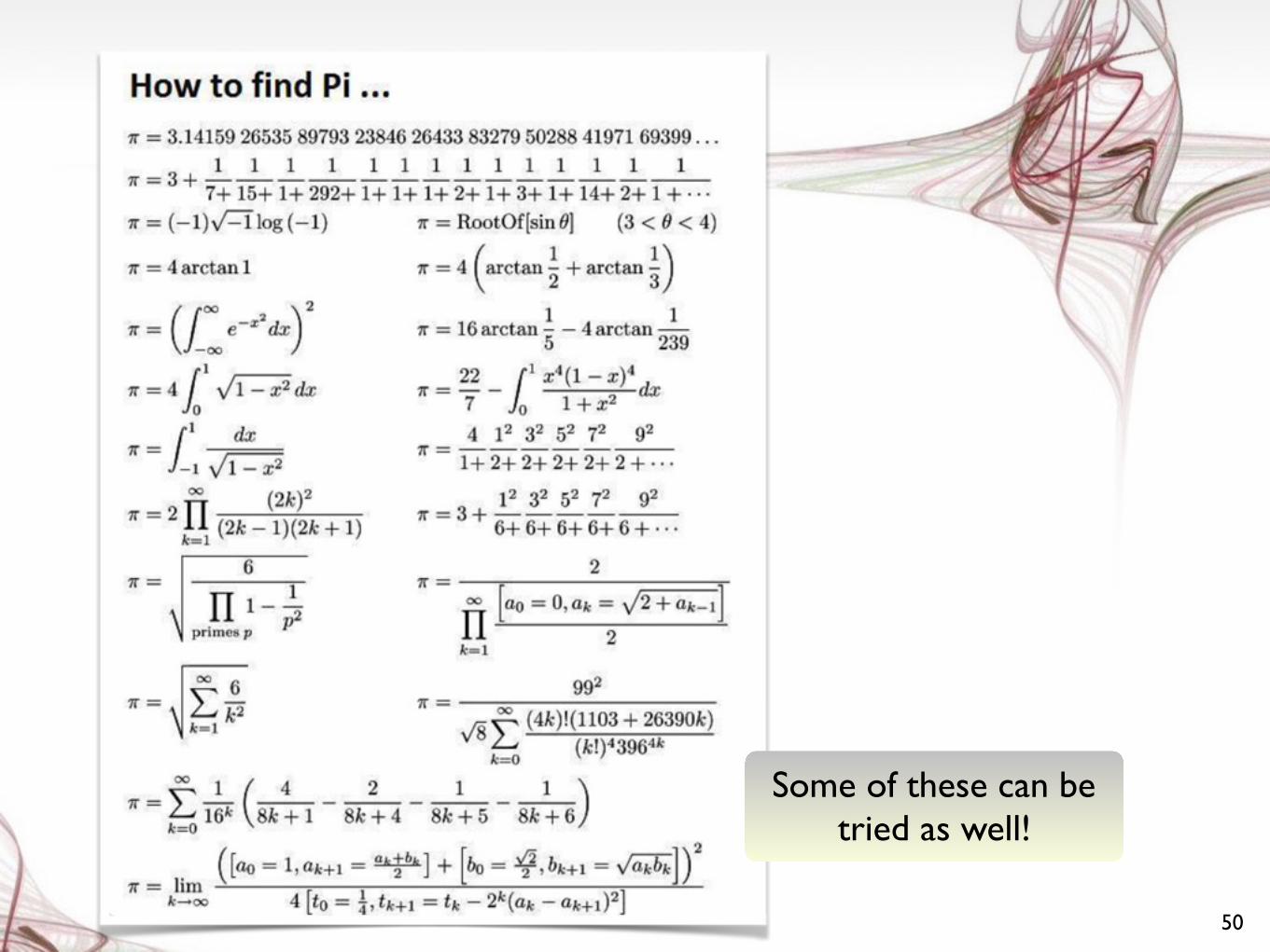
50

Some of these can be tried as well!

2019 introduction to numerical analysiskfjack/lecture/... · introduction to numerical analysis ......

Documents