numerical analysis i - pkudsec.pku.edu.cn/~tlu/na10/numericalanalysis.pdf · 1 introduction and...

Numerical Analysis I

Peter Philip∗

Lecture Notes

Originally Created for the Class of Winter Semester 2008/2009 at LMU Munich,

Revised and Extended for the Class of Winter Semester 2009/2010

January 27, 2010

Contents

1 Introduction and Motivation 4

2 Rounding and Error Analysis 8

2.1 Floating-Point Numbers Arithmetic, Rounding . . . . . . . . . . . . . . . 8

2.2 Rounding Errors . . . . . . . . . . . . . . . . . . . . . . . . . . . . . . . 12

2.3 Landau Symbols . . . . . . . . . . . . . . . . . . . . . . . . . . . . . . . 16

2.4 Operator Norms and Matrix Norms . . . . . . . . . . . . . . . . . . . . . 21

2.5 Condition of a Problem . . . . . . . . . . . . . . . . . . . . . . . . . . . . 28

3 Interpolation 38

3.1 Motivation . . . . . . . . . . . . . . . . . . . . . . . . . . . . . . . . . . . 38

3.2 Polynomial Interpolation . . . . . . . . . . . . . . . . . . . . . . . . . . . 39

3.2.1 Existence and Uniqueness . . . . . . . . . . . . . . . . . . . . . . 39

3.2.2 Newton’s Divided Difference Interpolation Formula . . . . . . . . 41

3.2.3 Error Estimates and the Mean Value Theorem for Divided Differ-ences . . . . . . . . . . . . . . . . . . . . . . . . . . . . . . . . . . 45

3.3 Hermite Interpolation . . . . . . . . . . . . . . . . . . . . . . . . . . . . . 48

3.4 The Weierstrass Approximation Theorem . . . . . . . . . . . . . . . . . . 56

∗E-Mail: [email protected]

1

CONTENTS 2

3.5 Spline Interpolation . . . . . . . . . . . . . . . . . . . . . . . . . . . . . . 59

3.5.1 Introduction . . . . . . . . . . . . . . . . . . . . . . . . . . . . . . 59

3.5.2 Linear Splines . . . . . . . . . . . . . . . . . . . . . . . . . . . . . 60

3.5.3 Cubic Splines . . . . . . . . . . . . . . . . . . . . . . . . . . . . . 61

4 Numerical Integration 69

4.1 Introduction . . . . . . . . . . . . . . . . . . . . . . . . . . . . . . . . . . 69

4.2 Quadrature Rules Based on Interpolating Polynomials . . . . . . . . . . . 73

4.3 Newton-Cotes Formulas . . . . . . . . . . . . . . . . . . . . . . . . . . . 76

4.3.1 Definition, Weights, Degree of Accuracy . . . . . . . . . . . . . . 76

4.3.2 Rectangle Rules (n = 0) . . . . . . . . . . . . . . . . . . . . . . . 79

4.3.3 Trapezoidal Rule (n = 1) . . . . . . . . . . . . . . . . . . . . . . . 80

4.3.4 Simpson’s Rule (n = 2) . . . . . . . . . . . . . . . . . . . . . . . . 80

4.3.5 Higher Order Newton-Cotes Formulas . . . . . . . . . . . . . . . . 82

4.4 Convergence of Quadrature Rules . . . . . . . . . . . . . . . . . . . . . . 82

4.5 Composite Newton-Cotes Quadrature Rules . . . . . . . . . . . . . . . . 85

4.5.1 Introduction, Convergence . . . . . . . . . . . . . . . . . . . . . . 85

4.5.2 Composite Rectangle Rules (n = 0) . . . . . . . . . . . . . . . . . 87

4.5.3 Composite Trapezoidal Rules (n = 1) . . . . . . . . . . . . . . . . 87

4.5.4 Composite Simpson’s Rules (n = 2) . . . . . . . . . . . . . . . . . 88

4.6 Gaussian Quadrature . . . . . . . . . . . . . . . . . . . . . . . . . . . . . 89

4.6.1 Introduction . . . . . . . . . . . . . . . . . . . . . . . . . . . . . . 89

4.6.2 Orthogonal Polynomials . . . . . . . . . . . . . . . . . . . . . . . 89

4.6.3 Gaussian Quadrature Rules . . . . . . . . . . . . . . . . . . . . . 93

5 Numerical Solution of Linear Systems 97

5.1 Motivation . . . . . . . . . . . . . . . . . . . . . . . . . . . . . . . . . . . 97

5.2 Gaussian Elimination and LU Decomposition . . . . . . . . . . . . . . . 98

5.2.1 Pivot Strategies . . . . . . . . . . . . . . . . . . . . . . . . . . . . 98

5.2.2 Gaussian Elimination via Matrix Multiplication and LU Decom-position . . . . . . . . . . . . . . . . . . . . . . . . . . . . . . . . 101

5.2.3 The Algorithm of LU Decomposition . . . . . . . . . . . . . . . . 110

5.3 QR Decomposition . . . . . . . . . . . . . . . . . . . . . . . . . . . . . . 112

CONTENTS 3

5.3.1 Definition and Motivation . . . . . . . . . . . . . . . . . . . . . . 112

5.3.2 QR Decomposition via Gram-Schmidt Orthogonalization . . . . . 113

5.3.3 QR Decomposition via Householder Reflections . . . . . . . . . . 115

6 Iterative Methods, Solution of Nonlinear Equations 115

6.1 Motivation: Fixed Points and Zeros . . . . . . . . . . . . . . . . . . . . . 115

6.2 Banach Fixed Point Theorem . . . . . . . . . . . . . . . . . . . . . . . . 116

6.3 Newton’s Method . . . . . . . . . . . . . . . . . . . . . . . . . . . . . . . 118

1 INTRODUCTION AND MOTIVATION 4

1 Introduction and Motivation

The central motivation of Numerical Analysis is to provide constructive and effectivemethods (so-called algorithms, see Def. 1.1 below) that reliably compute solutions (orsufficiently accurate approximations of solutions) to classes of mathematical problems.Moreover, such methods should also be efficient, i.e. one would like the algorithm tobe as quick as possible while one would also like it to use as little memory as possible.Frequently, both goals can not be achieved simultaneously: For example, one mightdecide to recompute intermediate results (which needs more time) to avoid storing them(which would require more memory) or vice versa. One typically also has a trade-off between accuracy and requirements for memory and execution time, where higheraccuracy means use of more memory and longer execution times.

Thus, one of the main tasks of Numerical Analysis consists of proving that a givenmethod is constructive, effective, and reliable. That a method is constructive, effective,and reliable means that, given certain hypotheses, it is guaranteed to converge to thesolution. This means, it either finds the solution in a finite number of steps, or, moretypically, given a desired error bound, within a finite number of steps, it approximatesthe true solution such that the error is less than the given bound. Proving error estimatesis another main task of Numerical Analysis and so is proving bounds on an algorithm’scomplexity, i.e. bounds on its use of memory (i.e. data) and run time (i.e. number ofsteps). Moreover, in addition to being convergent, for a method to be useful, it is ofcrucial importance that is also stable in the sense that a small perturbation of the inputdata does not destroy the convergence and results in, at most, a small increase of theerror. This is of the essence as, for most applied problems, the input data will not beexact, and most algorithms are subject to round-off errors.

Instead of a method, we will usually speak of an algorithm, by which we mean a “useful”method. To give a mathematically precise definition of the notion algorithm is beyondthe scope of this lecture (it would require an unjustifiably long detour into the field oflogic), but the following definition will be sufficient for our purposes.

Definition 1.1. An algorithm is a finite sequence of instructions for the solution of aclass of problems. Each instruction must be representable by a finite number of symbols.Moreover, an algorithm must be guaranteed to terminate after a finite number of steps.

Remark 1.2. Even though we here require an algorithm to terminate after a finitenumber of steps, in the literature, one sometimes omits this part from the definition.The question if a given method can be guaranteed to terminate after a finite number ofsteps is often tremendously difficult (sometimes even impossible) to answer.

Example 1.3. Let a, a0 ∈ R+ and consider the sequence (xn)n∈N0 defined recursivelyby

x0 := a0, xn+1 :=1

2

(xn +

a

xn

)for each n ∈ N0. (1.1)

It can be shown that, for each a, a0 ∈ R+, this sequence is well-defined (i.e. xn > 0 foreach n ∈ N0) and converges to

√a (this is Newton’s method, which we will study in a


later section, for the computation of the zero of the function f : R+ −→ R, f(x) :=x2 − a). The xn can be computed using the following finite sequence of instructions:

1 : x = a0 % store the number a0 in the variable x

2 : x = (x+ a/x)/2 % compute (x+ a/x)/2 and replace the

% contents of the variable x with the computed value

3 : goto 2 % continue with instruction 2

(1.2)

Even though the contents of the variable x will converge to√a, (1.2) does not constitute

an algorithm in the sense of Def. 1.1 since it does not terminate. To guarantee termi-nation and to make the method into an algorithm, one might introduce the followingmodification:

1 : ǫ = 10−10 ∗ a % store the number 10−10a in the variable ǫ

2 : x = a0 % store the number a0 in the variable x

3 : y = x % copy the contents of the variable x to

% the variable y to save the value for later use

4 : x = (x+ a/x)/2 % compute (x+ a/x)/2 and replace the

% contents of the variable x with the computed value

5 : if |x− y| > ǫ

then goto 3 % if |x− y| > ǫ, then continue with instruction 3

else quit % if |x− y| ≤ ǫ, then terminate the method

(1.3)

Now the convergence of the sequence guarantees that the method terminates withinfinitely many steps.

—

Another problem with regard to algorithms, that we already touched on in Example 1.3,is the implicit requirement of Def. 1.1 for an algorithm to be well-defined. That means,for every initial condition, given a number n ∈ N, the method has either terminatedafter m ≤ n steps, or it provides a (feasible!) instruction to carry out step number n+1.Such methods are called complete. Methods that can run into situations, where theyhave not reached their intended termination point, but can not carry out any furtherinstruction, are called incomplete. Algorithms must be complete! We illustrate the issuein the next example:

Example 1.4. Let a ∈ R \ {2} and N ∈ N. Define the following finite sequence ofinstructions:

1 : n = 1; x = a

2 : x = 1/(2 − x); n = n+ 1

3 : if n ≤ N

then goto 2

else quit

(1.4)


Consider what occurs for N = 10 and a = 54. The successive values contained in

the variable x are 54, 4

3, 3

2, 2. At this stage n = 4 ≤ N , i.e. instruction 3 tells the

method to continue with instruction 2. However, the denominator has become 0, andthe instruction has become meaningless. The following modification makes the methodcomplete and, thereby, an algorithm:

1 : n = 1; x = a

2 : if x 6= 2

then x = 1/(2 − x); n = n+ 1

else x = −5; n = n+ 1

3 : if n ≤ N

then goto 2

else quit

(1.5)

—

We can only expect to find stable algorithms if the underlying problem is sufficientlybenign. This leads to the following definition:

Definition 1.5. We say that a mathematical problem is well-posed provided that itssolutions enjoy the three benign properties of existence, uniqueness, and continuity withrespect to the input data. More precisely, given admissible input data, the problemmust have a unique solution (output), thereby providing a map between the set ofadmissible input data and (a superset of) the set of possible solutions. This map mustbe continuous with respect to suitable norms or metrics on the respective sets (smallchanges of the input data must only cause small changes in the solution). A problemwhich is not well-posed is called ill-posed.

—

We can thus add to the important tasks of Numerical Analysis mentioned earlier theadditional important tasks of investigating a problem’s well-posedness. Then, once well-posedness is established, the task is to provide a stable algorithm for its solution.

Example 1.6. (a) The problem “find a minimum of a given polynomial p : R −→ R”is inherently ill-posed: Depending on p, the problem has no solution (e.g. p(x) = x),a unique solution (e.g. p(x) = x2), finitely many solutions (e.g. p(x) = x2(x−1)2(x+2)2) or infinitely many solutions (e.g. p(x) = 1)).

(b) Frequently, one can transform an ill-posed problem into a well-posed problem, bychoosing an appropriate setting: Consider the problem “find a zero of f(x) =ax2 + c”. If, for example, one admits a, c ∈ R and looks for solutions in R, then theproblem is ill-posed as one has no solutions for ac > 0 and no solutions for a = 0,c 6= 0. Even for ac < 0, the problem is not well-posed as the solution is not alwaysunique. However, in this case, one can make the problem well-posed by considering


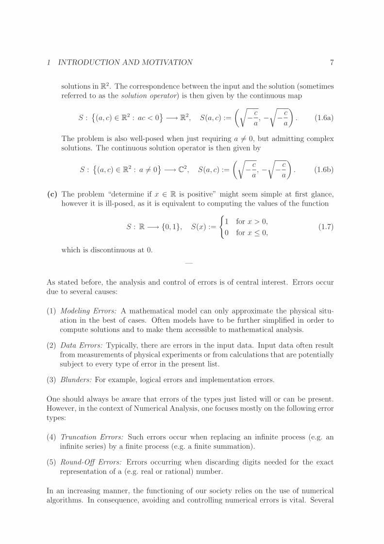
solutions in R2. The correspondence between the input and the solution (sometimesreferred to as the solution operator) is then given by the continuous map

S :{(a, c) ∈ R2 : ac < 0

}−→ R2, S(a, c) :=

(√− c

a, −√

− c

a

). (1.6a)

The problem is also well-posed when just requiring a 6= 0, but admitting complexsolutions. The continuous solution operator is then given by

S :{(a, c) ∈ R2 : a 6= 0

}−→ C2, S(a, c) :=

(√− c

a, −√

− c

a

). (1.6b)

(c) The problem “determine if x ∈ R is positive” might seem simple at first glance,however it is ill-posed, as it is equivalent to computing the values of the function

S : R −→ {0, 1}, S(x) :=

{1 for x > 0,

0 for x ≤ 0,(1.7)

which is discontinuous at 0.

—

As stated before, the analysis and control of errors is of central interest. Errors occurdue to several causes:

(1) Modeling Errors: A mathematical model can only approximate the physical situ-ation in the best of cases. Often models have to be further simplified in order tocompute solutions and to make them accessible to mathematical analysis.

(2) Data Errors: Typically, there are errors in the input data. Input data often resultfrom measurements of physical experiments or from calculations that are potentiallysubject to every type of error in the present list.

(3) Blunders: For example, logical errors and implementation errors.

One should always be aware that errors of the types just listed will or can be present.However, in the context of Numerical Analysis, one focuses mostly on the following errortypes:

(4) Truncation Errors: Such errors occur when replacing an infinite process (e.g. aninfinite series) by a finite process (e.g. a finite summation).

(5) Round-Off Errors: Errors occurring when discarding digits needed for the exactrepresentation of a (e.g. real or rational) number.

In an increasing manner, the functioning of our society relies on the use of numericalalgorithms. In consequence, avoiding and controlling numerical errors is vital. Several

2 ROUNDING AND ERROR ANALYSIS 8

examples of major disasters caused by numerical errors can be found on the followingweb page of D.N. Arnold at the University of Minnesota:http://www.ima.umn.edu/~arnold/disasters/

For a much more comprehensive list of numerical and related errors that had significantconsequences, see the web page of T. Huckle at TU Munich:http://www5.in.tum.de/~huckle/bugse.html

2 Rounding and Error Analysis

2.1 Floating-Point Numbers Arithmetic, Rounding

All the numerical problems considered in this class are related to the computation of(approximations of) real numbers. The b-adic representations of real numbers (seeAppendix A), in general, need infinitely many digits. However, computer memory canonly store a finite amount of data. This implies the need to introduce representationsthat use only strings of finite length and only a finite number of symbols. Clearly, givena supply of s ∈ N symbols and strings of length l ∈ N, one can represent a maximum ofsl <∞ numbers. The representation of this form most commonly used to approximatereal numbers is the so-called floating-point representation:

Definition 2.1. Let b ∈ N, b ≥ 2, l ∈ N, and N−, N+ ∈ Z with N− ≤ N+. Then, foreach

(x1, . . . , xl) ∈ {0, 1, . . . , b− 1}l, (2.1a)

N ∈ Z satisfying N− ≤ N ≤ N+, (2.1b)

the strings0 . x1x2 . . . xl · bN and − 0 . x1x2 . . . xl · bN (2.2)

are called floating-point representations of the (rational) numbers

x := bNl∑

ν=1

xνb−ν and − x, (2.3)

respectively, provided that x1 6= 0 if x 6= 0. For floating-point representations, b iscalled the radix (or base), 0 . x1 . . . xl (i.e. |x|/bN) is called the significand (or mantissaor coefficient), x1, . . . , xl are called the significant digits, and N is called the exponent.The number l is sometimes called the precision. Let fll(b,N−, N+) ⊆ Q denote the set ofall rational numbers that have a floating point representation of precision l with respectto base b and exponent between N− and N+.

Remark 2.2. If one restricts Def. 2.1 to the case N− = N+, then one obtains whatis known as fixed-point representations. However, for many applications, the requirednumbers vary over sufficiently many orders of magnitude to render fixed-point represen-tations impractical.


Remark 2.3. Given the assumptions of Def. 2.1, for the numbers in (2.3), it alwaysholds that

bN−−1 ≤ bN−1 ≤l∑

ν=1

xνbN−ν = |x| ≤ (b− 1)

l∑

ν=1

bN+−ν =: max(l, b, N+)Lem. A.2

< bN+ ,

(2.4)provided that x 6= 0. In other words:

fll(b,N−, N+) ⊆ Q ∩([−max(l, b, N+),−bN−−1] ∪ {0} ∪ [bN−−1,max(l, b, N+)]

). (2.5)

Obviously, fll(b,N−, N+) is not closed under arithmetic operations. A result of absolutevalue bigger than max(l, b, N+) is called an overflow, whereas a nonzero result of absolutevalue less than bN−−1 is called an underflow. In practice, the result of an underflow isusually replaced by 0.

Definition 2.4. Let b ∈ N, b ≥ 2, l ∈ N, N ∈ Z, and σ ∈ {−1, 1}. Then, given

x = σbN∞∑

ν=1

xνb−ν , (2.6)

where xν ∈ {0, 1, . . . , b− 1} for each ν ∈ N and x1 6= 0 for x 6= 0, define

rdl(x) :=

{σbN

∑lν=1 xνb

−ν for xl+1 < b/2,

σbN(b−l +∑l

ν=1 xνb−ν) for xl+1 ≥ b/2.

(2.7)

The number rdl(x) is called x rounded to l digits.

Remark 2.5. We note that the notation rdl(x) of Def. 2.4 is actually not entirely correct,since rdl is actually a function of the sequence (σ,N, x1, x2, . . . ) rather than of x: It canactually occur that rdl takes on different values for different representations of the samenumber x (for example, using decimal notation, consider x = 0.349 = 0.350, yieldingrd1(0.349) = 0.3 and rd1(0.350) = 0.4). However, from basic results on b-adic expansionsof real numbers (see Th. A.6), we know that x can have at most two different b-adicrepresentations and, for the same x, rdl(x) can vary at most bNb−l. Since always writingrdl(σ,N, x1, x2, . . . ) does not help with readability, and since writing rdl(x) hardly evercauses confusion as to what is meant in a concrete case, the abuse of notation introducedin Def. 2.4 is quite commonly employed.

Lemma 2.6. Let b ∈ N, b ≥ 2, l ∈ N. If x ∈ R is given by (2.6), then rdl(x) =σbN

′∑lν=1 x

′νb

−ν, where N ′ ∈ {N,N + 1} and x′ν ∈ {0, 1, . . . , b− 1} for each ν ∈ N andx′1 6= 0 for x 6= 0. In particular, rdl maps

⋃∞k=1 flk(b,N−, N+) into fll(b,N−, N+ + 1).

Proof. For xl+1 < b/2, there is nothing to prove. Thus, assume xl+1 ≥ b/2. Case (i):There exists ν ∈ {1, . . . , l} such that xν < b − 1. Then, letting ν0 ∈ {1, . . . , l} be thelargest index such that xν < b− 1, one finds N ′ = N and

x′ν =

xν for 1 ≤ ν < ν0,

xν0 + 1 for ν = ν0,

0 for ν0 < ν ≤ l.

(2.8a)


Case (ii): xν = b− 1 holds for each ν ∈ {1, . . . , l}. Then one obtains N ′ = N + 1,

x′ν :=

{1 for ν = 1,

0 for 1 < ν ≤ l,(2.8b)

thereby concluding the proof. �

Lemma 2.7. Let b ∈ N, b ≥ 2. Suppose

x = bN∞∑

ν=1

xνb−ν , y = bM

∞∑

ν=1

yνb−ν , (2.9)

where N,M ∈ Z; xν , yν ∈ {0, 1, . . . , b− 1} for each ν ∈ N; and x1, y1 6= 0.

(a) If N > M , then x ≥ y.

(b) If N = M and there is n ∈ N such that xn > yn and xν = yν for each ν ∈{1, . . . , n− 1}, then x ≥ y.

Proof. (a): One estimates

x− y = bN∞∑

ν=1

xνb−ν − bM

∞∑

ν=1

yνb−ν ≥ bN−1 − bN−1

∞∑

ν=1

(b− 1)b−ν

= bN−1 − bN−1(b− 1)

(1

1 − b−1− 1

)= 0. (2.10a)

(b): One estimates

x− y = bN∞∑

ν=1

xνb−ν − bM

∞∑

ν=1

yνb−ν = bN

∞∑

ν=n

xνb−ν − bN

∞∑

ν=n

yνb−ν

≥ bN−n − bN−n

∞∑

ν=1

(b− 1)b−ν as in (2.10a)= 0, (2.10b)

concluding the proof of the lemma. �

Lemma 2.8. Let b ∈ N, b ≥ 2, l ∈ N. Then, for each x, y ∈ R:

(a) rdl(x) = sgn(x) rdl(|x|).

(b) 0 ≤ x < y implies 0 ≤ rdl(x) ≤ rdl(y).

(c) 0 ≥ x > y implies 0 ≥ rdl(x) ≥ rdl(y).

Proof. (a): If x is given by (2.6), one obtains from (2.7):

rdl(x) = σ rdl

(bN

∞∑

ν=1

xνb−ν

)= sgn(x) rdl(|x|).


(b): Suppose x and y are given as in (2.9). Then Lem. 2.7(a) implies N ≤M .

Case xl+1 < b/2: In this case, according to (2.7),

rdl(x) = bNl∑

ν=1

xνb−ν . (2.11)

For N < M , we estimate

rdl(y) ≥ bMl∑

ν=1

yνb−ν

Lem. 2.7(a)

≥ bNl∑

ν=1

xνb−ν = rdl(x), (2.12)

which establishes the case. We claim that (2.12) also holds for N = M , now dueto Lem. 2.7(b): This is clear if xν = yν for each ν ∈ {1, . . . , l}. Otherwise, definen := min

{ν ∈ {1, . . . , l} : xν 6= yν

}. Then x < y and Lem. 2.7(b) yield xn < yn.

Moreover, another application of Lem. 2.7(b) then implies (2.12) for this case.

Case xl+1 ≥ b/2: In this case, according to Lem. 2.6,

rdl(x) = bN′

l∑

ν=1

x′νb−ν , (2.13)

where either N ′ = N and the x′ν are given by (2.8a), or N ′ = N +1 and the x′ν are givenby (2.8b). For N < M , we obtain

rdl(y) ≥ bMl∑

ν=1

yνb−ν

(∗)

≥ bN′

l∑

ν=1

x′νb−ν = rdl(x), (2.14)

where, for N ′ < M , (∗) holds by Lem. 2.7(a), and, for N ′ = N + 1 = M , (∗) holdsby (2.8b). It remains to consider N = M . If xν = yν for each ν ∈ {1, . . . , l}, thenx < y and Lem. 2.7(b) yield b/2 ≤ xl+1 ≤ yl+1, which, in turn, yields rdl(y) = rdl(x).Otherwise, once more define n := min

{ν ∈ {1, . . . , l} : xν 6= yν

}. As before, x < y and

Lem. 2.7(b) yield xn < yn. From Lem. 2.6, we obtain N ′ = N and that the x′ν are givenby (2.8a) with ν0 ≥ n. Then the values from (2.8a) show that (2.14) holds true onceagain.

(c) follows by combining (a) and (b). �

When composing floating point numbers of a fixed precision l ∈ N by means of arithmeticoperations such as ‘+’, ‘−’, ‘·’, and ‘:’, the exact result is usually not representable as afloating point number with the same precision l: For example, 0.434 ·104 +0.705 ·10−1 =0.43400705 · 104, which is not representable exactly with just 3 significant digits. Thus,when working with floating point numbers of a fixed precision, rounding will generallybe necessary.

The following Notation 2.9 makes sense for general real numbers x, y, but is intendedto be used with numbers from some fll(b,N−, N+), i.e. numbers given in floating pointrepresentation (in particular, with a finite precision).


Notation 2.9. Let b ∈ N, b ≥ 2. Assume x, y ∈ R are given in a form analogous to(2.6). We then define, for each l ∈ N,

x ⋄l y := rdl(x ⋄ y), (2.15)

where ⋄ can stand for any of the operations ‘+’, ‘−’, ‘·’, and ‘:’.

Remark 2.10. It follows from Lem. 2.6 that, given x, y ∈ fll(b,N−, N+), the result ofx ⋄l y as defined in (2.15) is either in fll(b,N−, N+) or an overflow.

Remark 2.11. The definition of (2.15) should only be taken as an example of howfloating-point operations can be realized. On concrete computer systems, the roundingoperations implemented can be different from the one considered here. However, it isthe property stated in Rem. 2.10 that one expects floating-point operations to satisfy.

Caveat 2.12. Unfortunately, the associative laws of addition and multiplication as wellas the law of distributivity are lost for arithmetic operations of floating-point numbers.More precisely, even if x, y, z ∈ fll(b,N−, N+) and one assumes that no overflow occurs,then there are examples, where (x+l y) +l z 6= x+l (y+l z), (x ·l y) ·l z 6= x ·l (y ·l z), andx ·l (y +l z) 6= x ·l y +l x ·l z (exercise).

Definition and Remark 2.13. Let b ∈ N, b ≥ 2, l ∈ N, and N−, N+ ∈ Z withN− ≤ N+. If there exists a smallest positive number ǫ ∈ fll(b,N−, N+) such that

1 +l ǫ 6= 1, (2.16)

then it is called the relative machine precision. It is an exercise to show that, forN+ < −l + 1, one has 1 +l y = 1 for every 0 < y ∈ fll(b,N−, N+), such that there is nopositive number in fll(b,N−, N+) satisfying (2.16), whereas, for N+ ≥ −l + 1:

ǫ =

{bN−−1 for −l + 1 < N−,

⌈b/2⌉b−l for −l + 1 ≥ N−

(for x ∈ R, ⌈x⌉ := min{k ∈ Z : x ≤ k} is called ceiling of x or x rounded up).

2.2 Rounding Errors

Definition 2.14. Let v ∈ R be the exact value and let a ∈ R be an approximation forv. The numbers

ea := |v − a|, er :=ea|v| (2.17)

are called the absolute error and the relative error, respectively, where the relative erroris only defined for v 6= 0. It can also be useful to consider variants of the absolute andrelative error, respectively, where one does not take the absolute value. Thus, in theliterature, one finds the definitions with and without the absolute value.


Proposition 2.15. Let b ∈ N be even, b ≥ 2, l ∈ N, N ∈ Z, and σ ∈ {−1, 1}. Supposex ∈ R is given by (2.6), i.e.

x = σbN∞∑

ν=1

xνb−ν , (2.18)

where xν ∈ {0, 1, . . . , b− 1} for each ν ∈ N and x1 6= 0 for x 6= 0,

(a) The absolute error of rounding to l digits satisfies

ea(x) =∣∣ rdl(x) − x

∣∣ ≤ bN−l

2.

(b) The relative error of rounding to l digits satisfies, for each x 6= 0,

er(x) =

∣∣ rdl(x) − x∣∣

|x| ≤ b−l+1

2.

(c) For each x 6= 0, one also has the estimate

∣∣ rdl(x) − x∣∣

| rdl(x)|≤ b−l+1

2.

Proof. (a): First, consider the case xl+1 < b/2: One computes

ea(x) =∣∣ rdl(x) − x

∣∣ = −σ(rdl(x) − x

)= bN

∞∑

ν=l+1

xνb−ν

= bN−l−1xl+1 + bN∞∑

ν=l+2

xνb−ν

b even, (A.3)

≤ bN−l−1

(b

2− 1

)+ bN−l−1 =

bN−l

2. (2.19a)

It remains to consider the case xl+1 ≥ b/2. In that case, one obtains

σ(rdl(x) − x

)= bN−l − bNxl+1b

−l−1 − bN∞∑

ν=l+2

xνb−ν

= bN−l−1(b− xl+1) − bN∞∑

ν=l+2

xνb−ν ≤ bN−l

2. (2.19b)

Due to 1 ≤ b− xl+1, one has bN−l−1 ≤ bN−l−1(b− xl+1). Therefore, bN∑∞

ν=l+2 xνb−ν ≤

bN−l−1 together with (2.19b) implies σ(rdl(x) − x

)≥ 0, i.e. ea(x) = σ

(rdl(x) − x

).

(b): Since x 6= 0, one has x1 ≥ 1. Thus, |x| ≥ bN−1. Then (a) yields

er =ea|x| ≤

bN−l b−N+1

2=b−l+1

2. (2.20)


(c): Again, x1 ≥ 1 as x 6= 0. Thus, (2.7) implies | rdl(x)| ≥ bN−1. This time, (a) yields

ea| rdl(x)|

≤ bN−l b−N+1

2=b−l+1

2, (2.21)

establishing the case and completing the proof of the proposition. �

Corollary 2.16. In the situation of Prop. 2.15, let, for x 6= 0:

ǫl(x) :=rdl(x) − x

x, η l(x) :=

rdl(x) − x

rdl(x). (2.22)

Then

max{|ǫl(x)|, |ηl(x)|

}≤ b−l+1

2=: τ l. (2.23)

The number τ l is called the relative computing precision of floating-point arithmetic withl significant digits. �

Remark 2.17. From the definitions of ǫl(x) and η l(x) in (2.22), one immediately obtainsthe relations

rdl(x) = x(1 + ǫl(x)

)=

x

1 − η l(x)for x 6= 0. (2.24)

In particular, according to (2.15), one has for floating-point operations (for x ⋄ y 6= 0):

x ⋄l y = rdl(x ⋄ y) = (x ⋄ y)(1 + ǫl(x ⋄ y)

)=

x ⋄ y1 − η l(x ⋄ y)

. (2.25)

—

One can use the formulas of Rem. 2.17 to perform what is sometimes called a forwardanalysis of the rounding error. This technique is illustrated in the next example.

Example 2.18. Let x := 0.9995 · 100 and y := −0.9984 · 100. Computing the sum withprecision 3 yields

rd3(x) +3 rd3(y) = 0.100 · 101 +3 (−0.998 · 100) = rd3(0.2 · 10−2) = 0.2 · 10−2. (2.26)

Letting ǫ := ǫ3(rd3(x) + rd3(y)), applying the formulas of Rem. 2.17 provides:

rd3(x) +3 rd3(y)(2.25)=

(rd3(x) + rd3(y)

)(1 + ǫ)

(2.24)=

(x(1 + ǫ3(x)) + y(1 + ǫ3(y))

)(1 + ǫ)

= (x+ y) + ea, (2.27)

whereea = x

(ǫ+ ǫ3(x)(1 + ǫ)

)+ y(ǫ+ ǫ3(y)(1 + ǫ)

). (2.28)


Using (2.22) and plugging in the numbers yields:

ǫ =rd3(x) +3 rd3(y) −

(rd3(x) + rd3(y)

)

rd3(x) + rd3(y)=

0.002 − 0.002

0.002= 0, (2.29a)

ǫ3(x) =1 − 0.9995

0.9995=

1

1999= 0.00050 . . . , (2.29b)

ǫ3(y) =−0.998 + 0.9984

−0.9984= − 1

2496= −0.00040 . . . , (2.29c)

ea = xǫ3(x) + yǫ3(y) = 0.0005 + 0.0004 = 0.0009. (2.29d)

The corresponding relative error is

er =ea

|x+ y| =0.0009

0.0011=

9

11= 0.81. (2.30)

Thus, er is much larger than both er(x) and er(y). This is an example of subtractivecancellation of digits, which can occur when subtracting numbers that are almost iden-tical. If possible, such situations should be avoided in practice (cf. Examples 2.19 and2.20 below).

Example 2.19. Let us generalize the situation of Example 2.18 to general x, y ∈ R\{0}and a general precision l ≥ 2. The formulas in (2.27) and (2.28) remain valid if onereplaces 3 by l. Moreover, with b = 10, one obtains from (2.23):

|ǫ| ≤ 0.5 · 10−l+1 ≤ 0.5 · 10−1 = 0.05. (2.31a)

Thus,|ea| ≤ |x|

(ǫ+ 1.05|ǫl(x)|

)+ |y|

(ǫ+ 1.05|ǫl(y)|

), (2.31b)

and

er =|ea|

|x+ y| ≤|x|

|x+ y|(|ǫ| + 1.05|ǫl(x)|

)+

|y||x+ y|

(|ǫ| + 1.05|ǫl(y)|

). (2.31c)

One can now distinguish three (not completely disjoint) cases:

(a) If |x + y| < max{|x|, |y|} (in particular, if sgn(x) = − sgn(y)), then er is typicallylarger (potentially much larger, as in Example 2.18) than |ǫl(x)| and |ǫl(y)|. Sub-tractive cancellation falls into this case. If possible, this should be avoided (cf.Example 2.20 below).

(b) If sgn(x) = sgn(y), then |x+ y| = |x| + |y|, implying

er ≤ |ǫ| + 1.05 max{|ǫl(x)|, |ǫl(y)|

}

i.e. the relative error is at most of the same order of magnitude as the number|ǫ| + max

{|ǫl(x)|, |ǫl(y)|

}.


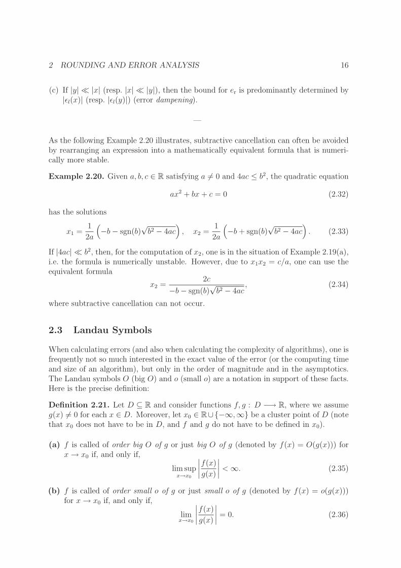
(c) If |y| ≪ |x| (resp. |x| ≪ |y|), then the bound for er is predominantly determined by|ǫl(x)| (resp. |ǫl(y)|) (error dampening).

—

As the following Example 2.20 illustrates, subtractive cancellation can often be avoidedby rearranging an expression into a mathematically equivalent formula that is numeri-cally more stable.

Example 2.20. Given a, b, c ∈ R satisfying a 6= 0 and 4ac ≤ b2, the quadratic equation

ax2 + bx+ c = 0 (2.32)

has the solutions

x1 =1

2a

(−b− sgn(b)

√b2 − 4ac

), x2 =

1

2a

(−b+ sgn(b)

√b2 − 4ac

). (2.33)

If |4ac| ≪ b2, then, for the computation of x2, one is in the situation of Example 2.19(a),i.e. the formula is numerically unstable. However, due to x1x2 = c/a, one can use theequivalent formula

x2 =2c

−b− sgn(b)√b2 − 4ac

, (2.34)

where subtractive cancellation can not occur.

2.3 Landau Symbols

When calculating errors (and also when calculating the complexity of algorithms), one isfrequently not so much interested in the exact value of the error (or the computing timeand size of an algorithm), but only in the order of magnitude and in the asymptotics.The Landau symbols O (big O) and o (small o) are a notation in support of these facts.Here is the precise definition:

Definition 2.21. Let D ⊆ R and consider functions f, g : D −→ R, where we assumeg(x) 6= 0 for each x ∈ D. Moreover, let x0 ∈ R∪{−∞,∞} be a cluster point of D (notethat x0 does not have to be in D, and f and g do not have to be defined in x0).

(a) f is called of order big O of g or just big O of g (denoted by f(x) = O(g(x))) forx→ x0 if, and only if,

lim supx→x0

∣∣∣∣f(x)

g(x)

∣∣∣∣ <∞. (2.35)

(b) f is called of order small o of g or just small o of g (denoted by f(x) = o(g(x)))for x→ x0 if, and only if,

limx→x0

∣∣∣∣f(x)

g(x)

∣∣∣∣ = 0. (2.36)


As mentioned before, O and o are known as Landau symbols.

Proposition 2.22. We consider the setting of Def. 2.21 and provide the following equiv-alent characterizations of the Landau symbols:

(a) f(x) = O(g(x)) for x→ x0 if, and only if, there exist C, δ > 0 such that

∣∣∣∣f(x)

g(x)

∣∣∣∣ ≤ C for each x ∈ D \ {x0} with

|x− x0| < δ for x0 ∈ R,

x > δ for x0 = ∞,

x < −δ for x0 = −∞.

(2.37)

(b) f(x) = o(g(x)) for x → x0 if, and only if, for every C > 0, there exists δ > 0 suchthat (2.37) holds.

Proof. (a): First, suppose that (2.35) holds, and let M := lim supx→x0

∣∣∣f(x)g(x)

∣∣∣, C := 1 + M .

Consider the case x0 ∈ R. If there were no δ > 0 such that (2.37) holds, then, foreach δn := 1/n, n ∈ N, there were some xn ∈ D \ {x0} with |xn − x0| < δn and

yn :=∣∣∣f(xn)

g(xn)

∣∣∣ > C = 1 + M , implying lim supn→∞

yn ≥ 1 + M > M , in contradiction

to (2.35). The cases x0 = ∞ and x0 = −∞ are handled analogously (e.g., one canreplace δn := 1/n by δn := n and δn := −n, respectively). Conversely, if there existC, δ > 0 such that (2.37) holds true, then, for each sequence (xn)n∈N in D \ {x0} such

that limn→∞ xn = x0, one has that the sequence (yn)n∈N with yn :=∣∣∣f(xn)

g(xn)

∣∣∣ can not have

a cluster point larger than C (only finitely many of the xn are not in the neighborhoodof x0 determined by δ). Thus lim sup

n→∞yn ≤ C, thereby implying (2.35).

(b): There is nothing to prove, since the assertion that, for every C > 0, there existsδ > 0 such that (2.37) holds, is precisely the definition of the notation in (2.36). �

Proposition 2.23. Again, we consider the setting of Def. 2.21. In addition, for use insome of the following assertions, we introduce functions f1, f2, g1, g2 : D −→ R, wherewe assume g1(x) 6= 0 and g2(x) 6= 0 for each x ∈ D.

(a) Suppose |f | ≤ |g| in some neighborhood of x0, i.e. there exists ǫ > 0 such that

|f(x)| ≤ |g(x)| for each x ∈ D \ {x0} with

|x− x0| < ǫ for x0 ∈ R,

x > ǫ for x0 = ∞,

x < −ǫ for x0 = −∞.

(2.38)

Then f(x) = O(g(x)) for x→ x0.

(b) f(x) = O(f(x)) for x→ x0, but not f(x) = o(f(x)) for x→ x0 (assuming f 6= 0).


(c) If f(x) = O(g(x)) (resp. f(x) = o(g(x))) for x→ x0, and if |f1| ≤ |f | and |g| ≤ |g1|in some neighborhood of x0 (i.e. if there exists ǫ > 0 such that

|f1(x)| ≤ |f(x)|, |g(x)| ≤ |g1(x)| for each x ∈ D \ {x0}

with

|x− x0| < ǫ for x0 ∈ R,

x > ǫ for x0 = ∞,

x < −ǫ for x0 = −∞

,(2.39)

then f1(x) = O(g1(x)) (resp. f1(x) = o(g1(x))) for x→ x0.

(d) f(x) = o(g(x)) for x→ x0 implies f(x) = O(g(x)) for x→ x0.

(e) If α ∈ R \ {0}, then for x→ x0:

αf(x) = O(g(x)) ⇒ f(x) = O(g(x)), (2.40a)

αf(x) = o(g(x)) ⇒ f(x) = o(g(x)), (2.40b)

f(x) = O(αg(x)) ⇒ f(x) = O(g(x)), (2.40c)

f(x) = o(αg(x)) ⇒ f(x) = o(g(x)). (2.40d)

(f) For x→ x0:

f(x) = O(g1(x)) and g1(x) = O(g2(x)) implies f(x) = O(g2(x)), (2.41a)

f(x) = o(g1(x)) and g1(x) = o(g2(x)) implies f(x) = o(g2(x)). (2.41b)

(g) For x→ x0:

f1(x) = O(g(x)) and f2(x) = O(g(x)) implies f1(x) + f2(x) = O(g(x)),(2.42a)

f1(x) = o(g(x)) and f2(x) = o(g(x)) implies f1(x) + f2(x) = o(g(x)).(2.42b)

(h) For x→ x0:

f1(x) = O(g1(x)) and f2(x) = O(g2(x)) implies f1(x)f2(x) = O(g1(x)g2(x)),(2.43a)

f1(x) = o(g1(x)) and f2(x) = o(g2(x)) implies f1(x)f2(x) = o(g1(x)g2(x)).(2.43b)

(i) For x→ x0:

f(x) = O(g1(x)g2(x)) ⇒ f(x)

g1(x)= O(g2(x)), (2.44a)

f(x) = o(g1(x)g2(x)) ⇒ f(x)

g1(x)= o(g2(x)). (2.44b)


Proof. (a): The hypothesis implies

lim supx→x0

∣∣∣∣f(x)

g(x)

∣∣∣∣ ≤ lim supx→x0

∣∣∣∣g(x)

g(x)

∣∣∣∣ = 1 <∞. (2.45a)

(b): If f = g, then

lim supx→x0

∣∣∣∣f(x)

g(x)

∣∣∣∣ = limx→x0

∣∣∣∣f(x)

g(x)

∣∣∣∣ = 1. (2.45b)

Since 0 6= 1 < ∞, one has f(x) = O(f(x)) for x → x0, but not f(x) = o(f(x)) forx→ x0.

(c): The assertions follow, for example, by applying Prop. 2.22: Since∣∣∣f1(x)g1(x)

∣∣∣ ≤∣∣∣f(x)

g(x)

∣∣∣ in

the ǫ-neighborhood of x0 as given in (2.39), for f(x) = O(g(x)) (resp. f(x) = o(g(x))),(2.37) is valid for f1 and g1 if one replaces δ by min{δ, ǫ} (where, for f(x) = o(g(x)), δdoes, in general, depend on C).

(d): If the limit in (2.36) exists, then it coincides with the limit superior. It is thereforeimmediate that (2.36) implies (2.35).

(e): Everything follows immediately from the fact that multiplication with α and 1/α,respectively, commutes with taking the limit and the limit superior in (2.36) and (2.35),respectively.

(f): If, for x→ x0, f(x) = O(g1(x)) and g1(x) = O(g2(x)), then

0 ≤M1 := lim supx→x0

∣∣∣∣f(x)

g1(x)

∣∣∣∣ <∞ and 0 ≤M2 := lim supx→x0

∣∣∣∣g1(x)

g2(x)

∣∣∣∣ <∞, (2.45c)

implying

lim supx→x0

∣∣∣∣f(x)

g2(x)

∣∣∣∣ = lim supx→x0

∣∣∣∣f(x)

g1(x)

∣∣∣∣

∣∣∣∣g1(x)

g2(x)

∣∣∣∣ ≤M1M2 <∞. (2.45d)

If, for x→ x0, f(x) = o(g1(x)) and g1(x) = o(g2(x)), then

limx→x0

∣∣∣∣f(x)

g2(x)

∣∣∣∣ = limx→x0

∣∣∣∣f(x)

g1(x)

∣∣∣∣ limx→x0

∣∣∣∣g1(x)

g2(x)

∣∣∣∣ = 0. (2.45e)

(g): If, for x→ x0, f1(x) = O(g(x)) and f2(x) = O(g(x)), then

lim supx→x0

∣∣∣∣f1(x) + f2(x)

g(x)


∣∣∣∣f1(x)

g(x)

∣∣∣∣+ lim supx→x0

∣∣∣∣f2(x)

g(x)

∣∣∣∣ <∞. (2.45f)

If, for x→ x0, f1(x) = o(g(x)) and f2(x) = o(g(x)), then

limx→x0

∣∣∣∣f1(x) + f2(x)

g(x)

∣∣∣∣ = limx→x0

∣∣∣∣f1(x)

g(x)

∣∣∣∣+ limx→x0

∣∣∣∣f2(x)

g(x)

∣∣∣∣ = 0. (2.45g)

(h): If, for x→ x0, f1(x) = O(g1(x)) and f2(x) = O(g2(x)), then

lim supx→x0

∣∣∣∣f1(x)f2(x)

g1(x)g2(x)


∣∣∣∣f1(x)

g1(x)

∣∣∣∣ lim supx→x0

∣∣∣∣f2(x)

g2(x)

∣∣∣∣ <∞. (2.45h)


If, for x→ x0, f1(x) = o(g1(x)) and f2(x) = o(g2(x)), then

limx→x0

∣∣∣∣f1(x)f2(x)

g1(x)g2(x)

∣∣∣∣ = limx→x0

∣∣∣∣f1(x)

g1(x)

∣∣∣∣ limx→x0

∣∣∣∣f2(x)

g2(x)

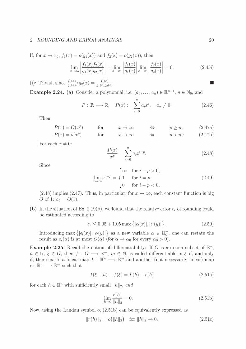
∣∣∣∣ = 0. (2.45i)

(i): Trivial, since f1(x)g1(x)

/g2(x) = f1(x)g1(x)g2(x)

. �

Example 2.24. (a) Consider a polynomial, i.e. (a0, . . . , an) ∈ Rn+1, n ∈ N0, and

P : R −→ R, P (x) :=n∑

i=0

aixi, an 6= 0. (2.46)

Then

P (x) = O(xp) for x→ ∞ ⇔ p ≥ n, (2.47a)

P (x) = o(xp) for x→ ∞ ⇔ p > n : (2.47b)

For each x 6= 0:P (x)

xp=

n∑

i=0

aixi−p. (2.48)

Since

limx→∞

xi−p =

∞ for i− p > 0,

1 for i = p,

0 for i− p < 0,

(2.49)

(2.48) implies (2.47). Thus, in particular, for x→ ∞, each constant function is bigO of 1: a0 = O(1).

(b) In the situation of Ex. 2.19(b), we found that the relative error er of rounding couldbe estimated according to

er ≤ 0.05 + 1.05 max{|ǫl(x)|, |ǫl(y)|

}. (2.50)

Introducing max{|ǫl(x)|, |ǫl(y)|

}as a new variable α ∈ R+

0 , one can restate theresult as er(α) is at most O(α) (for α → α0 for every α0 > 0).

Example 2.25. Recall the notion of differentiability: If G is an open subset of Rn,n ∈ N, ξ ∈ G, then f : G −→ Rm, m ∈ N, is called differentiable in ξ if, and onlyif, there exists a linear map L : Rn −→ Rm and another (not necessarily linear) mapr : Rn −→ Rm such that

f(ξ + h) − f(ξ) = L(h) + r(h) (2.51a)

for each h ∈ Rn with sufficiently small ‖h‖2, and

limh→0

r(h)

‖h‖2

= 0. (2.51b)

Now, using the Landau symbol o, (2.51b) can be equivalently expressed as

‖r(h)‖2 = o(‖h‖2

)for ‖h‖2 → 0. (2.51c)


Example 2.26. Let I ⊆ R be an open interval and a, x ∈ I, x 6= a. If m ∈ N0 andf ∈ Cm+1(I), then

f(x) = Tm(x, a) +Rm(x, a), (2.52a)

where

Tm(x, a) :=m∑

k=0

f (k)(a)

k!(x−a)k = f(a)+f ′(a)(x−a)+f ′′(a)

2!(x−a)2+· · ·+f (m)(a)

m!(x−a)m

(2.52b)is the mth Taylor polynomial and

Rm(x, a) :=f (m+1)(θ)

(m+ 1)!(x− a)m+1 with some suitable θ ∈]x, a[ (2.52c)

is the Lagrange form of the remainder term. Since the continuous function f (m+1) isbounded on each compact interval [a, y], y ∈ I, (2.52) imply

f(x) − Tm(x, a) = O((x− a)m+1

)(2.53)

for x→ x0 for each x0 ∈ I.

2.4 Operator Norms and Matrix Norms

When working in more general vector spaces than R, errors are measured by moregeneral norms than the absolute value (we already briefly encountered this in Example2.25). A special class of norms of importance to us is the class of norms defined onlinear maps between normed vector spaces. In terms of Numerical Analysis, we willmostly be interested in linear maps between Rn and Rm, i.e. in linear maps given byreal matrices. However, introducing the relevant notions for linear maps between generalnormed vector spaces does not provide much additional difficulty, and, hopefully, evensome extra clarity.

Definition 2.27. Let A : X −→ Y be a linear map between two normed vector spaces(X, ‖·‖X) and (Y, ‖·‖Y ). Then A is called bounded if, and only if, A maps bounded setsto bounded sets, i.e. if, and only if, A(B) is a bounded subset of Y for each boundedB ⊆ X. The vector space of all bounded linear maps between X and Y is denoted byL(X,Y ).

Definition 2.28. Let A : X −→ Y be a linear map between two normed vector spaces(X, ‖ · ‖X) and (Y, ‖ · ‖Y ). The number

‖A‖ := sup

{‖Ax‖Y

‖x‖X

: x ∈ X, x 6= 0

}

= sup{‖Ax‖Y : x ∈ X, ‖x‖X = 1

}∈ [0,∞] (2.54)

is called the operator norm of A induced by ‖ · ‖X and ‖ · ‖Y (strictly speaking, the termoperator norm is only justified if the value is finite, but it is often convenient to use theterm in the generalized way defined here).


In the special case, where X = Rn, Y = Rm, and A is given via a real m × n matrix,the operator norm is also called matrix norm.

—

From now on, the space index of a norm will usually be suppressed, i.e. we write just‖ · ‖ instead of both ‖ · ‖X and ‖ · ‖Y .

Theorem 2.29. For a linear map A : X −→ Y between two normed vector spaces(X, ‖ · ‖) and (Y, ‖ · ‖), the following statements are equivalent:

(a) A is bounded.

(b) ‖A‖ <∞.

(c) A is Lipschitz continuous.

(d) A is continuous.

(e) There is x0 ∈ X such that A is continuous at x0.

Proof. Since every Lipschitz continuous map is continuous and since every continuousmap is continuous at every point, “(c) ⇒ (d) ⇒ (e)” is clear.

“(e) ⇒ (c)”: Let x0 ∈ X be such that A is continuous at x0. Thus, for each ǫ > 0, thereis δ > 0 such that ‖x− x0‖ < δ implies ‖Ax−Ax0‖ < ǫ. As A is linear, for each x ∈ Xwith ‖x‖ < δ, one has ‖Ax‖ = ‖A(x+ x0)−Ax0‖ < ǫ, due to ‖x+ x0 − x0‖ = ‖x‖ < δ.Moreover, one has ‖(δx)/2‖ ≤ δ/2 < δ for each x ∈ X with ‖x‖ ≤ 1. Letting L := 2ǫ/δ,this means that ‖Ax‖ = ‖A((δx)/2)‖/(δ/2) < 2ǫ/δ = L for each x ∈ X with ‖x‖ ≤ 1.Thus, for each x, y ∈ X with x 6= y, one has

‖Ax− Ay‖ = ‖A(x− y)‖ = ‖x− y‖∥∥∥∥A(

x− y

‖x− y‖

)∥∥∥∥ < L ‖x− y‖. (2.55)

Together with the fact that ‖Ax−Ay‖ ≤ ‖x− y‖ is trivially true for x = y, this showsthat A is Lipschitz continuous.

“(c) ⇒ (b)”: As A is Lipschitz continuous, there exists L ∈ R+0 such that ‖Ax−Ay‖ ≤

L ‖x − y‖ for each x, y ∈ X. Considering the special case y = 0 and ‖x‖ = 1 yields‖Ax‖ ≤ L ‖x‖ = L, implying ‖A‖ ≤ L <∞.

“(b) ⇒ (c)”: Let ‖A‖ <∞. We will show

‖Ax− Ay‖ ≤ ‖A‖ ‖x− y‖ for each x, y ∈ X. (2.56)

For x = y, there is nothing to prove. Thus, let x 6= y. One computes

‖Ax− Ay‖‖x− y‖ =

∥∥∥∥A(

x− y

‖x− y‖

)∥∥∥∥ ≤ ‖A‖ (2.57)

as∥∥∥ x−y‖x−y‖

∥∥∥ = 1, thereby establishing (2.56).


“(b) ⇒ (a)”: Let ‖A‖ <∞ and let M ⊆ X be bounded. Then there is r > 0 such thatM ⊆ Br(0). Moreover, for each 0 6= x ∈M :

‖Ax‖‖x‖ =

∥∥∥∥A(

x

‖x‖

)∥∥∥∥ ≤ ‖A‖ (2.58)

as∥∥∥ x‖x‖

∥∥∥ = 1. Thus ‖Ax‖ ≤ ‖A‖‖x‖ ≤ r‖A‖, showing that A(M) ⊆ Br‖A‖(0). Thus,

A(M) is bounded, thereby establishing the case.

“(a) ⇒ (b)”: Since A is bounded, it maps the bounded set B1(0) ⊆ X into somebounded subset of Y . Thus, there is r > 0 such that A(B1(0)) ⊆ Br(0) ⊆ Y . Inparticular, ‖Ax‖ < r for each x ∈ X satisfying ‖x‖ = 1, showing ‖A‖ ≤ r <∞. �

Remark 2.30. For linear maps between finite-dimensional spaces, the equivalent prop-erties of Th. 2.29 always hold: Each linear map A : Rn −→ Rm, (n,m) ∈ N2, iscontinuous (this follows, for example, from the fact that each such map is (trivially)differentiable, and every differentiable map is continuous). In particular, each linearmap A : Rn −→ Rm, has all the equivalent properties of Th. 2.29.

Theorem 2.31. Let X and Y be normed vector spaces.

(a) The operator norm does, indeed, constitute a norm on the set of bounded linearmaps L(X,Y ).

(b) If A ∈ L(X,Y ), then ‖A‖ is the smallest Lipschitz constant for A, i.e. ‖A‖ is aLipschitz constant for A and ‖Ax − Ay‖ ≤ L ‖x − y‖ for each x, y ∈ X implies‖A‖ ≤ L.

Proof. (a): If A = 0, then, in particular, Ax = 0 for each x ∈ X with ‖x‖ = 1, implying‖A‖ = 0. Conversely, ‖A‖ = 0 implies Ax = 0 for each x ∈ X with ‖x‖ = 1. But thenAx = ‖x‖A(x/‖x‖) = 0 for every 0 6= x ∈ X, i.e. A = 0. Thus, the operator norm ispositive definite. If A ∈ L(X,Y ), λ ∈ R, and x ∈ X, then

∥∥(λA)x∥∥ =

∥∥A(λx)∥∥ =

∥∥λ(Ax)∥∥ = |λ|

∥∥Ax∥∥, (2.59)

yielding

‖λA‖ = sup{‖(λA)x‖ : x ∈ X, ‖x‖ = 1

}= sup

{|λ| ‖Ax‖ : x ∈ X, ‖x‖ = 1

}

= |λ| sup{‖Ax‖ : x ∈ X, ‖x‖ = 1

}= |λ| ‖A‖, (2.60)

showing that the operator norm is homogeneous of degree 1. Finally, if A,B ∈ L(X,Y )and x ∈ X, then

‖(A+B)x‖ = ‖Ax+Bx‖ ≤ ‖Ax‖ + ‖Bx‖, (2.61)

yielding

‖A+B‖ = sup{‖(A+B)x‖ : x ∈ X, ‖x‖ = 1

}

≤ sup{‖Ax‖ + ‖Bx‖ : x ∈ X, ‖x‖ = 1

}

≤ sup{‖Ax‖ : x ∈ X, ‖x‖ = 1

}+ sup

{‖Bx‖ : x ∈ X, ‖x‖ = 1

}

= ‖A‖ + ‖B‖, (2.62)


showing that the operator norm also satisfies the triangle inequality, thereby completingthe verification that it is, indeed, a norm.

(b): That ‖A‖ is a Lipschitz constant for A was already shown in the proof of “(b) ⇒(c)” of Th. 2.29. Now let L ∈ R+

0 be such that ‖Ax−Ay‖ ≤ L ‖x−y‖ for each x, y ∈ X.Specializing to y = 0 and ‖x‖ = 1 implies ‖Ax‖ ≤ L ‖x‖ = L, showing ‖A‖ ≤ L. �

Remark 2.32. Even though it is beyond the scope of the present lecture, let us mentionas an outlook that one can show that L(X,Y ) with the operator norm is a Banach space(i.e. a complete normed vector space) provided that Y is a Banach space (even if X isnot a Banach space).

Lemma 2.33. If Id : X −→ X, Id(x) := x, is the identity map on a normed vectorspace X, then ‖ Id ‖ = 1 (in particular, the operator norm of a unit matrix is always 1).Caveat: In principle, one can consider two different norms on X simultaneously, andthen the operator norm of the identity can differ from 1.

Proof. If ‖x‖ = 1, then ‖ Id(x)‖ = ‖x‖ = 1. �

Lemma 2.34. Let X,Y, Z be normed vector spaces and consider linear maps A ∈L(X,Y ), B ∈ L(Y, Z). Then

‖BA‖ ≤ ‖B‖ ‖A‖. (2.63)

Proof. Let x ∈ X with ‖x‖ = 1. If Ax = 0, then ‖B(A(x))‖ = 0 ≤ ‖B‖ ‖A‖. If Ax 6= 0,then one estimates

∥∥B(Ax)∥∥ = ‖Ax‖

∥∥∥∥B(

Ax

‖Ax‖

)∥∥∥∥ ≤ ‖A‖ ‖B‖, (2.64)

thereby establishing the case. �

Example 2.35. Let m,n ∈ N and let A : Rn −→ Rm be the linear map given by them× n matrix (aij)(i,j)∈{1,...,m}×{1,...,n}. Then

‖A‖∞ := max

{n∑

j=1

|aij| : i ∈ {1, . . . ,m}}

(2.65a)

is called the row sum norm of A, and

‖A‖1 := max

{m∑

i=1

|aij| : j ∈ {1, . . . , n}}

(2.65b)

is called the column sum norm of A. It is an exercise to show that ‖A‖∞ is the operatornorm induced if Rn and Rm are endowed with the ∞-norm (see (B.3b)), and ‖A‖1 isthe operator norm induced if Rn and Rm are endowed with the 1-norm (see (B.3a)).

Notation 2.36. Let m,n ∈ N and let A = (aij)(i,j)∈{1,...,m}×{1,...,n} be a real m × nmatrix.


(a) By A∗ we denote the adjoint matrix of A, and by At := (aji)(j,i)∈{1,...,n}×{1,...,m} (ann × m matrix) we denote the transpose of A. Recall that, for real matrices, A∗

and At are identical, but for complex matrices, one has A∗ = (aji), where aji is thecomplex conjugate of aij.

(b) If m = n, then

trA :=n∑

i=1

aii (2.66)

denotes the trace of A.

Remark 2.37. Let m,n ∈ N and let A = (aij)(i,j)∈{1,...,m}×{1,...,n} be a real m×n matrix.Then:

tr(A∗A) = tr

(m∑

k=1

akiakj

)

(i,j)∈{1,...,n}2

=n∑

i=1

m∑

k=1

|aki|2, (2.67a)

tr(AA∗) = tr

(n∑

k=1

aikajk

)

(i,j)∈{1,...,m}2

=m∑

i=1

n∑

k=1

|aik|2. (2.67b)

Since the sums in (2.67a) and (2.67b) are identical, we have shown

tr(A∗A) = tr(AA∗). (2.68)

Definition and Remark 2.38. Let m,n ∈ N. If A is a real m × n matrix, then let‖A‖2 denote the operator norm induced by the Euclidean norms on Rm and Rn. Thisnorm is also known as the spectral norm of A (cf. Th. 2.44 below).

Caveat: ‖A‖2 is not(!) the 2-norm on Rmn, which is known as the Frobenius norm orthe Hilbert-Schmidt norm (see Example C.7). As it turns, for n,m > 1, the Frobeniusnorm is not induced by norms on Rm and Rn at all (for a proof see Appendix C).

Unfortunately, there is no formula as simple as the ones in (2.65) for the computationof the operator norm ‖A‖2 induced by the Euclidean norms. However, ‖A‖2 is oftenimportant, which is related to the fact that the Euclidean norm is induced by theEuclidean scalar product. We will see below, that the value of ‖A‖2 is related to theeigenvalues of A∗A.

—

We recall three important notions and then two important results from Linear Algebra:

Definition 2.39. Let n ∈ N and let A = (aij) be a real n× n matrix.

(a) A is called symmetric if, and only if, A = At, i.e. if, and only if, aij = aji for each(i, j) ∈ {1, . . . , n}2.

(b) A is called positive semidefinite if, and only if, xtAx ≥ 0 for each x ∈ Rn.


(c) A is called positive definite if, and only if, A is positive semidefinite and xtAx =0 ⇔ x = 0, i.e. if, and only if, xtAx > 0 for each 0 6= x ∈ Rn.

Theorem 2.40. If n ∈ N and A is a real n × n matrix, then A has precisely n, ingeneral complex, eigenvalues λi ∈ C if every eigenvalue is counted with its (algebraic)multiplicity (i.e. the multiplicity of the corresponding zero of the characteristic polyno-mial χA(λ) = det(λ Id−A) of A – it equals the geometric multiplicity (i.e. the dimensionof the eigenspace ker(λi Id−A)) if, and only if, A is diagonalizable). �

Theorem 2.41. If n ∈ N and A is a real, symmetric, and positive semidefinite n × nmatrix, then all eigenvalues λi of A are real and nonnegative: λi ∈ R+

0 . Moreover, thereis an orthonormal basis (v1, . . . , vn) of Rn such that vi is an eigenvector for λi, i.e., inparticular,

Avi = λivi, (2.69a)

vtivj = vi · vj =

{0 for i 6= j,

1 for i = j(2.69b)

for each i, j ∈ {1, . . . , n}. �

Lemma 2.42. Let m,n ∈ N and let A = (aij) be a real m× n matrix. Then A∗A is asymmetric and positive semidefinite n× n matrix, whereas AA∗ is a symmetric m×mmatrix.

Proof. Since (A∗)∗ = A, it suffices to consider A∗A. That A∗A is a symmetric n × nmatrix is immediately evident from the representation given in (2.67a) (since akiakj =akjaki). Moreover, if x ∈ Rn, then xtA∗Ax = (Ax)t(Ax) = ‖Ax‖2

2 ≥ 0, showing thatA∗A is positive semidefinite. �

Definition 2.43. In view of Th. 2.40, we define, for each n ∈ N and each real n × nmatrix A:

r(A) := max{|λ| : λ ∈ C and λ is eigenvalue of A

}. (2.70)

The number r(A) is called the spectral radius of A.

Theorem 2.44. Let m,n ∈ N. If A is a real m×n matrix, then its spectral norm ‖A‖2

(i.e. the operator norm induced by the Euclidean norms on Rm and Rn) satisfies

‖A‖2 =√r(A∗A). (2.71a)

If m = n and A is symmetric (i.e. A∗ = A), then ‖A‖2 is also given by the followingsimpler formula:

‖A‖2 = r(A). (2.71b)

Proof. According to Lem. 2.42, A∗A is a symmetric and positive semidefinite n × nmatrix. Then Th. 2.41 yields real nonnegative eigenvalues λ1, . . . , λn ≥ 0 and a corre-sponding orthonormal basis (v1, . . . , vn) of eigenvectors satisfying (2.69) with A replacedby A∗A, in particular,

A∗Avi = λivi for each i ∈ {1, . . . , n}. (2.72)


As (v1, . . . , vn) is a basis of Rn, for each x ∈ Rn, there are numbers x1, . . . , xn ∈ R suchthat x =

∑ni=1 xivi. Thus, one computes

‖Ax‖22 = (Ax) · (Ax) = xtA∗Ax =

(n∑

i=1

xivi

)·(

n∑

i=1

xiλivi

)

=n∑

i=1

λix2i ≤ r(A∗A)

n∑

i=1

x2i = r(A∗A)‖x‖2

2, (2.73)

proving ‖A‖2 ≤√r(A∗A). To verify the remaining inequality, let λ := r(A∗A) be the

largest of the nonnegative λi, and let v := vi be the corresponding eigenvector from theorthonormal basis. Then ‖v‖2 = 1 and choosing x = v in (2.73) yields ‖Av‖2

2 = r(A∗A),thereby proving ‖A‖2 ≥

√r(A∗A) and completing the proof of (2.71a). It remains to

consider the case where A = A∗. Then A∗A = A2 and since

Av = λv ⇒ A2v = λ2v, (2.74)

Th. 2.40 impliesr(A2) = r(A)2. (2.75)

Thus,‖A‖2 =

√r(A∗A) =

√r(A2) = r(A), (2.76)


Caveat 2.45. It is not admissible to use the simpler formula (2.71b) for nonsymmetric

n× n matrices: For example, for A :=

(0 10 1

), one has

A∗A =

(0 01 1

)(0 10 1

)=

(0 00 2

),

such that 1 = r(A) 6=√

2 =√r(A∗A) = ‖A‖2.

Lemma 2.46. Let n ∈ N. Then

‖y‖2 = max{v · y : v ∈ Rn and ‖v‖2 = 1

}for each y ∈ Rn. (2.77)

Proof. Let v ∈ Rn such that ‖v‖2 = 1. One estimates, using the Cauchy-Schwarzinequality,

v · y ≤ |v · y| ≤ ‖v‖2‖y‖2 = ‖y‖2. (2.78a)

Note that (2.77) is trivially true for y = 0. If y 6= 0, then letting w := y/‖y‖2 yields‖w‖2 = 1 and

w · y = y · y/‖y‖2 = ‖y‖2. (2.78b)

Together, (2.78a) and (2.78b) establish (2.77). �

Proposition 2.47. Let m,n ∈ N. If A is a real m × n matrix, then ‖A‖2 = ‖A∗‖2

and, in particular, r(A∗A) = r(AA∗). This allows to use the simpler (smaller) matrixof A∗A and AA∗ to compute ‖A‖2 (see Example 2.49 below).


Proof. One calculates

‖A‖2 = max{‖Ax‖2 : x ∈ Rn and ‖x‖2 = 1

}

(2.77)= max

{v · Ax : v, x ∈ Rn and ‖v‖2 = ‖x‖2 = 1

}

= max{(A∗v) · x : v, x ∈ Rn and ‖v‖2 = ‖x‖2 = 1

}

(2.77)= max

{‖A∗v‖2 : v ∈ Rn and ‖v‖2 = 1

}

= ‖A∗‖2, (2.79)

proving the proposition. �

Remark 2.48. One can actually show more than we did in Prop. 2.47: The eigenvalues(including multiplicities) of A∗A and AA∗ are always identical, except that the larger ofthe two matrices (if any) can have additional eigenvalues of value 0.

Example 2.49. Consider A :=

(1 0 1 00 1 1 0

). One obtains

AA∗ =

(2 11 2

), A∗A =

1 0 1 00 1 1 01 1 2 00 0 0 0

. (2.80)

So one would tend to compute the eigenvalues using AA∗. One finds λ1 = 1 and λ2 = 3.Thus, r(AA∗) = 3 and ‖A‖2 =

√3.

2.5 Condition of a Problem

We are now ready to exploit our acquired knowledge of operator norms to error analysis.The general setting is the following: The input is given in some normed vector space X(e.g. Rn) and the output is likewise a vector lying in some normed vector space Y (e.g.Rm). The solution operator, i.e. the map f between input and output, is some functionf defined on an open subset of X. The goal in this section is to study the behavior ofthe output given small changes (errors) of the input.

Definition 2.50. LetX and Y be normed vector spaces, U ⊆ X open, and f : U −→ Y .Fix x ∈ U \ {0} such that f(x) 6= 0 and δ > 0 such that Bδ(x) = {x ∈ X : ‖x − x‖ <δ} ⊆ U . We call (the problem represented by the solution operator) f well-conditionedin Bδ(x) if, and only if, there exists K ≥ 0 such that

‖f(x) − f(x)‖‖f(x)‖ ≤ K

‖x− x‖‖x‖ for every x ∈ Bδ(x). (2.81)

If f is well-conditioned in Bδ(x), then we define K(δ) := K(f, x, δ) to be the smallestnumber K ∈ R+

0 such that (2.81) is valid. If there exists δ > 0 such that f is well-conditioned in Bδ(x), then f is called well-conditioned at x.


Definition and Remark 2.51. We remain in the situation of Def. 2.50 and notice that0 < α ≤ β ≤ δ implies Bα(x) ⊆ Bβ(x) ⊆ Bδ(x), and, thus 0 ≤ K(α) ≤ K(β) ≤ K(δ).In consequence, the following definition makes sense if f is well-conditioned at x:

krel := krel(f, x) := limα→0

K(α). (2.82)

The number krel ∈ R+0 is called the relative condition of (the problem represented by the

solution operator) f at x.

Remark 2.52. The smaller krel, the more well-behaved is the problem in the vicinityof x, where stability corresponds more or less to krel < 100.

Remark 2.53. Let us compare the newly introduced notion of f being well-conditionedwith some other regularity notions for f . For example, if f is Lipschitz continuous inBδ(x), then f is clearly well-conditioned in Bδ(x). The converse is not true as, forexample, t 7→

√t is well-conditioned in B1(1) =]0, 2[, but not Lipschitz continuous on

B1(1). On the other hand, (2.81) does imply continuity in x. Once again, the converseis not true as, for example, t 7→ 1 +

√|t− 1| is continuous in 1, but it is not well-

conditioned in any Bδ(1) with δ > 0. In particular, a problem can be well-posed in thesense of Def. 1.5 without being well-conditioned. On the other hand if f is everywherewell-conditioned, then it is also well-posed. In that sense well-conditionedness is strongerthan well-posedness. However, one should also note that we defined well-conditionednessas a local property and we didn’t allow x = 0 and f(x) = 0, whereas well-posedness wasdefined as a global property.

Theorem 2.54. Let m,n ∈ N, let U ⊆ Rn be open, and assume that f : U −→ Rm

is continuously differentiable: f ∈ C1(U,Rm). If 0 6= x ∈ U and f(x) 6= 0, then f iswell-conditioned at x and

krel = ‖Df(x)‖ ‖x‖‖f(x)‖ , (2.83)

where Df(x) : Rn −→ Rm is the (total) derivative of f in x (a linear map represented bythe Jacobian Jf (x)). In (2.83), any norm on Rn and Rm will work as long as ‖Df(x)‖is the corresponding induced operator norm.

Proof. Choose δ > 0 sufficiently small such that Bδ(x) ⊆ U . Since f ∈ C1(U,Rm), wecan apply Taylor’s theorem. Recall that its lowest order version with the remainderterm in integral form states that, for each h ∈ Bδ(0) (which implies x+ h ∈ Bδ(x)), thefollowing holds:

f(x+ h) = f(x) +

∫ 1

0

Df(x+ th

)(h) dt . (2.84)

If x ∈ Bδ(x), then we can let h := x− x, which permits to restate (2.84) in the form

f(x) − f(x) =

∫ 1

0

Df((1 − t)x+ tx

)(x− x) dt . (2.85)


This allows to estimate the norm as follows:∥∥f(x) − f(x)

∥∥ =

∥∥∥∥∫ 1

0

Df((1 − t)x+ tx

)(x− x) dt

∥∥∥∥Th. D.5

≤∫ 1

0

∥∥∥Df((1 − t)x+ tx

)(x− x)

∥∥∥ dt

≤∫ 1

0

∥∥∥Df((1 − t)x+ tx

)∥∥∥ ‖x− x‖ dt

≤ sup{∥∥Df(y)

∥∥ : y ∈ Bδ(x)}‖x− x‖

= S(δ)‖x− x‖ (2.86)

with S(δ) := sup{∥∥Df(y)

∥∥ : y ∈ Bδ(x)}. This implies

∥∥f(x) − f(x)∥∥

∥∥f(x)∥∥ ≤ ‖x‖∥∥f(x)

∥∥S(δ)‖x− x‖‖x‖ (2.87)

and, therefore,

K(δ) ≤ ‖x‖∥∥f(x)∥∥S(δ). (2.88)

The hypothesis that f is continuously differentiable implies limy→xDf(y) = Df(x),which implies limy→x ‖Df(y)‖ = ‖Df(x)‖ (continuity of the norm, cf. Rem. B.19(b)),which, in turn, implies limδ→0 S(δ) = ‖Df(x)‖. Since, also, limδ→0K(δ) = krel, (2.88)yields

krel ≤ ‖Df(x)‖ ‖x‖‖f(x)‖ . (2.89)

In still remains to prove the inverse inequality. To that end, choose v ∈ Rn such that‖v‖ = 1 and ∥∥Df(x)(v)

∥∥ =∥∥Df(x)

∥∥ (2.90)

(such a vector v must exist due to the fact that the continuous function y 7→ ‖Df(x)(y)‖must attain its max on the compact unit sphere S1(0) – note that this argument doesnot work in infinite-dimensional spaces, where S1(0) is not compact). For 0 < ǫ < δconsider x := x+ǫv. Then ‖x−x‖ = ǫ < δ, i.e. x ∈ Bδ(x). In particular, x is admissiblein (2.85), which provides

f(x) − f(x) = ǫ

∫ 1

0

Df((1 − t)x+ tx

)(v) dt

= ǫDf(x)(v) + ǫ

∫ 1

0

(Df((1 − t)x+ tx

)−Df(x)

)(v) dt . (2.91)

Once again using ‖x − x‖ = ǫ as well as the triangle inequality in the form ‖a + b‖ ≥‖a‖ − ‖b‖, we obtain from (2.91) and (2.90):

∥∥f(x) − f(x)∥∥

∥∥f(x)∥∥

≥ ‖x‖∥∥f(x)∥∥

(∥∥Df(x)∥∥−

∫ 1

0

∥∥∥Df((1 − t)x+ tx

)−Df(x)

∥∥∥ dt

) ‖x− x‖‖x‖ . (2.92)


Thus,

K(ǫ) ≥ ‖x‖∥∥f(x)∥∥(∥∥Df(x)

∥∥− T (ǫ)), (2.93)

where

T (ǫ) := sup

{∫ 1

0

∥∥∥Df((1 − t)x+ tx

)−Df(x)

∥∥∥ dt : x ∈ Bǫ(x)

}. (2.94)

Since Df is continuous in x, for each α > 0, there is ǫ > 0 such that ‖y−x‖ ≤ ǫ implies‖Df(y) −Df(x)‖ < α. Thus, since ‖(1 − t)x + tx − x‖ = t ‖x − x‖ ≤ ǫ for x ∈ Bǫ(x)and t ∈ [0, 1], one obtains

T (ǫ) ≤∫ 1

0

α dt = α, (2.95)

implyinglimǫ→0

T (ǫ) = 0. (2.96)

In particular, we can take limits in (2.93) to get

krel ≥‖x‖∥∥f(x)

∥∥∥∥Df(x)

∥∥. (2.97)

Finally, (2.97) together with (2.89) completes the proof of (2.83). �

Example 2.55. (a) Let us investigate the condition of the problem of multiplication,by considering

f : R2 −→ R, f(x, y) := xy, Df(x, y) = (y, x). (2.98)

Using the Euclidean norm on R2, one obtains (exercise) for each (x, y) ∈ R2 suchthat xy 6= 0,

krel(x, y) =|x||y| +

|y||x| . (2.99)

Thus, we see that the relative condition explodes if |x| ≫ |y| or |x| ≪ |y|. Since onecan also show (exercise) that f is well-conditioned in Bδ(x, y) for each δ > 0, wesee that multiplication is numerically stable if, and only if, |x| and |y| are roughlyof the same order of magnitude.

(b) Analogous to (a), we now investigate division, i.e.

g : R ×(R \ {0}

)−→ R, g(x, y) :=

x

y, Dg(x, y) =

(1

y, − x

y2

). (2.100)

Once again using the Euclidean norm on R2, one obtains from (2.83) that, for each(x, y) ∈ R2 such that xy 6= 0,

krel(x, y) = ‖Dg(x, y)‖2‖(x, y)‖2

|g(x, y)| =|y||x|√x2 + y2

√1

y2+x2

y4

=1

|x|√x2 + y2

√

1 +x2

y2=x2 + y2

|x||y| =|x||y| +

|y||x| , (2.101)


i.e. the relative condition is the same as for multiplication. In particular, divisionalso becomes unstable if |x| ≫ |y| or |x| ≪ |y|, while krel(x, y) remains small if |x|and |y| are of the same order of magnitude. However, we now again investigate ifg is well-conditioned in Bδ(x, y), δ > 0, and here we find an important differencebetween division and multiplication. For δ ≥ |y|, it is easy to see that g is not well-conditioned in Bδ(x, y): For each n ∈ N, let zn := (x, y

n). Then ‖(x, y) − zn‖2 =

(1 − 1n)|y| < |y| ≤ δ, but

∣∣∣∣x

y− xn

y

∣∣∣∣ = (n− 1)|x||y| → ∞ for n→ ∞. (2.102)

For 0 < δ < |y|, the result is different: Suppose |y| ≤ |y| − δ. Then∥∥(x, y) − (x, y)

∥∥2≥ |y − y| ≥ |y| − |y| ≥ δ. (2.103)

Thus, (x, y) ∈ Bδ(x, y) implies |y| > |y|−δ. In consequence, one estimates, for each(x, y) ∈ Bδ(x, y),

∣∣g(x, y) − g(x, y)∣∣ =

∣∣∣∣x

y− x

y

∣∣∣∣ ≤∣∣∣∣x

y− x

y

∣∣∣∣+∣∣∣∣x

y− x

y

∣∣∣∣ =

∣∣∣∣x

yy

∣∣∣∣ |y − y| +∣∣∣∣1

y

∣∣∣∣ |x− x|

≤ max

{ |x||y|(|y| − δ)

,1

|y| − δ

} ∥∥(x, y) − (x, y)∥∥

1

≤ Cmax

{ |x||y|(|y| − δ)

,1

|y| − δ

} ∥∥(x, y) − (x, y)∥∥

2(2.104)

for some suitable C ∈ R+, showing that g is well-conditioned in Bδ(x, y) for 0 <δ < |y|. The significance of the present example lies in its demonstration that theknowledge of krel(x, y) alone is not enough to determine the numerical stability of gat (x, y): Even though krel(x, y) can remain bounded for y → 0, the problem is thatthe neighborhood Bδ(x, y), where division is well-conditioned, becomes arbitrarilysmall. Thus, without an effective bound (from below) on Bδ(x, y), the knowledgeof krel(x, y) can be completely useless and even misleading.

As another important example, we consider the problem of solving the linear systemAx = b with an invertible real n× n matrix A. Before studying the problem systemati-cally using the notion of well-conditionedness, let us look at a particular example thatillustrates a typical instability that can occur:

Example 2.56. Consider the linear system

Ax = b (2.105)

for the unknown x ∈ R4 with

A :=

10 7 8 77 5 6 58 6 10 97 5 9 10

, b :=

32233331

. (2.106)


One finds that the solution is

x :=

1111

. (2.107)

If instead of b, we are given the following perturbed b,

b :=

32.122.933.130.9

, (2.108)

where the absolute error is 0.1 and relative error is even smaller, then the correspondingsolution is

x :=

9.2−12.64.5−1.1

, (2.109)

in no way similar to the solution to b. In particular, the absolute and relative errorshave been hugely amplified.

One might suspect that the issue behind the instability lies in A being “almost” singularsuch that applying A−1 is similar to dividing by a small number. However, that is notthe case, as we have

A−1 =

25 −41 10 −6−41 68 −17 1010 −17 5 −3−6 10 −3 2

. (2.110)

We will see shortly that the actual reason behind the instability is the range of eigen-values of A, in particular, the relation between the largest and the smallest eigenvalue.One has:

λ1 ≈ 0.010, λ2 ≈ 0.843, λ3 ≈ 3.86, λ4 ≈ 30.3,λ4

λ1

≈ 2984. (2.111)

For our systematic investigation of this problem, we now apply (2.83) to the generalsituation:

Example 2.57. Let A be an invertible real n × n matrix, n ∈ N and consider theproblem of solving the linear system Ax = b. Then the solution operator is

f : Rn −→ Rn, f(b) := A−1b, Df(b) = A−1. (2.112)

Fixing some norm on Rn and using the induced matrix norm, we obtain from (2.83)that, for each 0 6= b ∈ Rn:

krel(b) = ‖Df(b)‖ ‖b‖‖f(b)‖ = ‖A−1‖ ‖b‖

‖A−1b‖x:=A−1b

= ‖A−1‖ ‖Ax‖‖x‖ ≤ ‖A‖‖A−1‖. (2.113)


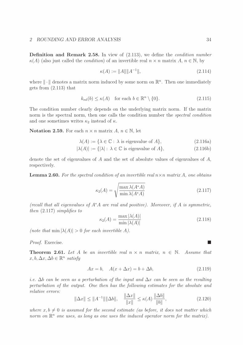
Definition and Remark 2.58. In view of (2.113), we define the condition numberκ(A) (also just called the condition) of an invertible real n× n matrix A, n ∈ N, by

κ(A) := ‖A‖‖A−1‖, (2.114)

where ‖ · ‖ denotes a matrix norm induced by some norm on Rn. Then one immediatelygets from (2.113) that

krel(b) ≤ κ(A) for each b ∈ Rn \ {0}. (2.115)

The condition number clearly depends on the underlying matrix norm. If the matrixnorm is the spectral norm, then one calls the condition number the spectral conditionand one sometimes writes κ2 instead of κ.

Notation 2.59. For each n× n matrix A, n ∈ N, let

λ(A) := {λ ∈ C : λ is eigenvalue of A}, (2.116a)

|λ(A)| := {|λ| : λ ∈ C is eigenvalue of A}, (2.116b)

denote the set of eigenvalues of A and the set of absolute values of eigenvalues of A,respectively.

Lemma 2.60. For the spectral condition of an invertible real n×n matrix A, one obtains

κ2(A) =

√maxλ(A∗A)

minλ(A∗A)(2.117)

(recall that all eigenvalues of A∗A are real and positive). Moreover, if A is symmetric,then (2.117) simplifies to

κ2(A) =max |λ(A)|min |λ(A)| (2.118)

(note that min |λ(A)| > 0 for each invertible A).

Proof. Exercise. �

Theorem 2.61. Let A be an invertible real n × n matrix, n ∈ N. Assume thatx, b,∆x,∆b ∈ Rn satisfy

Ax = b, A(x+ ∆x) = b+ ∆b, (2.119)

i.e. ∆b can be seen as a perturbation of the input and ∆x can be seen as the resultingperturbation of the output. One then has the following estimates for the absolute andrelative errors:

‖∆x‖ ≤ ‖A−1‖‖∆b‖, ‖∆x‖‖x‖ ≤ κ(A)

‖∆b‖‖b‖ , (2.120)

where x, b 6= 0 is assumed for the second estimate (as before, it does not matter whichnorm on Rn one uses, as long as one uses the induced operator norm for the matrix).


Proof. Since A is linear, (2.119) implies A(∆x) = ∆b, i.e. ∆x = A−1(∆b), which alreadyyields the first estimate in (2.120). For x, b 6= 0, the first estimate together with Ax = beasily implies the second:

‖∆x‖‖x‖ ≤ ‖A−1‖ ‖∆b‖

‖b‖‖Ax‖‖x‖ , (2.121)


Example 2.62. Suppose we want to find out how much we can perturb b in the problem

Ax = b, A :=

(1 21 1

), b :=

(14

), (2.122)

if the resulting relative error er in x is to be less than 10−2 with respect to the ∞-norm.From (2.120), we know

er ≤ κ(A)‖∆b‖∞‖b‖∞

= κ(A)‖∆b‖∞

4. (2.123)

Moreover, since A−1 =

(−1 21 −1

), from (2.114) and (2.65a), we obtain

κ(A) = ‖A‖∞‖A−1‖∞ = 3 · 3 = 9. (2.124)

Thus, if the perturbation ∆b satisfies ‖∆b‖∞ < 4/900 ≈ 0.0044, then er <94· 4900

= 10−2.

Remark 2.63. Note that (2.120) is a much stronger and more useful statement thanthe krel(b) ≤ κ(A) of (2.113). The relative condition only provides a bound in the limitof smaller and smaller neighborhoods of b and without providing any information onhow small the neighborhood actually has to be (one can estimate the amplification ofthe error in x provided that the error in b is very small). On the other hand, (2.120)provides an effective control of the absolute and relative errors without any restrictionswith regard to the size of the error in b (it holds for each ∆b).

—

Let us come back to the instability observed in Example 2.56 and determine its actualcause. Suppose A is any symmetric invertible real n×n matrix, λmin, λmax ∈ λ(A) suchthat |λmin| = min |λ(A)|, |λmax| = max |λ(A)|. Let vmin and vmax be eigenvectors for λmin

and λmax, respectively, satisfying ‖vmin‖ = ‖vmax‖ = 1. The most unstable behavior ofAx = b occurs if b = vmax and b is perturbed in the direction of vmin, i.e. b := b+ ǫ vmin,ǫ > 0. The solution to Ax = b is x = λ−1

maxvmax, whereas the solution to Ax = b is

x = A−1(vmax + ǫ vmin) = λ−1maxvmax + ǫλ−1

minvmin. (2.125)

Thus, the resulting relative error in the solution is

‖x− x‖‖x‖ = ǫ

|λmax||λmin|

, (2.126)


while the relative error in the input was merely

‖b− b‖‖b‖ = ǫ. (2.127)

This shows that, in the worst case, the relative error in b can be amplified by a factorof κ2(A) = |λmax|/|λmin|, and that is exactly what had occurred in Example 2.56.

—

Before concluding this section, we study a generalization of the problem from (2.119).Now, in addition to a perturbation of the right-hand side b, we also allow a perturbationof the matrix A by a matrix ∆A:

Ax = b, (A+ ∆A)(x+ ∆x) = b+ ∆b. (2.128)

We would now like to control ∆x in terms of ∆b and ∆A.

Remark 2.64. The set of invertible real n × n matrices is open in the set of all realn×n matrices (which is the same as Rn2

, where all norms are equivalent) – this follows,for example, from the determinant being a continuous map (even a polynomial) fromRn2

into R, which implies that det−1(R \ {0}) must be open. Thus, if A in (2.128) isinvertible and ‖∆A‖ is sufficiently small, then A+ ∆A must also be invertible.

Lemma 2.65. Let n ∈ N, consider some norm on Rn and the induced matrix norm onthe set of real n×n matrices. If B is a real n×n matrix such that ‖B‖ < 1, then Id +Bis invertible and

‖(Id +B)−1‖ ≤ 1

1 − ‖B‖ . (2.129)

Proof. For each x ∈ Rn:

‖(Id +B)x‖ ≥ ‖x‖ − ‖Bx‖ ≥ ‖x‖ − ‖B‖ ‖x‖ = (1 − ‖B‖) ‖x‖, (2.130)

showing that x 6= 0 implies (Id +B)x 6= 0, i.e. Id +B is invertible. Fixing y ∈ Rn andapplying (2.130) with x := (Id−B)−1y yields

‖(Id +B)−1y‖ ≤ 1

1 − ‖B‖ ‖y‖, (2.131)

thereby proving (2.129) and concluding the proof of the lemma. �

Lemma 2.66. Let n ∈ N, consider some norm on Rn and the induced matrix norm onthe set of real n× n matrices. If A and ∆A are real n× n matrices such A is invertibleand ‖∆A‖ < ‖A−1‖−1, then A+ ∆A is invertible and

‖(A+ ∆A)−1‖ ≤ 1

‖A−1‖−1 − ‖∆A‖ . (2.132)

Moreover,

‖∆A‖ ≤ 1

2‖A−1‖ ⇒ ‖(A+ ∆A)−1 − A−1‖ ≤ C‖∆A‖, (2.133)

where the constant can be chosen as C := 2‖A−1‖2.


Proof. We can write A + ∆A = A(Id +A−1∆A). As ‖A−1∆A‖ ≤ ‖A−1‖ ‖∆A‖ < 1,Lem. 2.65 yields that Id +A−1∆A is invertible. Since A is also invertible, so is A+ ∆A.Moreover,

‖(A+ ∆A)−1‖ =∥∥(Id +A−1∆A)−1A−1

∥∥ (2.129)

≤ ‖A−1‖1 − ‖A−1∆A‖ ≤ ‖A−1‖

1 − ‖A−1‖ ‖∆A‖ ,(2.134)

proving (2.132). One easily verifies the identity

(A+ ∆A)−1 − A−1 = −(A+ ∆A)−1(∆A)A−1, (2.135)

which yields, for ‖∆A‖ ≤ 12‖A−1‖

,

‖(A+ ∆A)−1 − A−1‖ ≤ ‖(A+ ∆A)−1‖ ‖∆A‖ ‖A−1‖(2.134)

≤ ‖A−1‖ ‖∆A‖ ‖A−1‖1 − ‖A−1‖ ‖∆A‖

≤ 2 ‖A−1‖2 ‖∆A‖, (2.136)

proving (2.133). �

Theorem 2.67. As in Lem. 2.66, let n ∈ N, consider some norm on Rn and the inducedmatrix norm on the set of real n×n matrices, and let A and ∆A be real n×n matricessuch A is invertible and ‖∆A‖ < ‖A−1‖−1. Moreover, assume b, x,∆b,∆x ∈ Rn satisfy

Ax = b, (A+ ∆A)(x+ ∆x) = b+ ∆b. (2.137)

Then one has the following bound for the relative error:

‖∆x‖‖x‖ ≤ κ(A)

1 − ‖A−1‖ ‖∆A‖

(‖∆A‖‖A‖ +

‖∆b‖‖b‖

). (2.138)

Proof. The equations (2.137) imply

(A+ ∆A)(∆x) = ∆b− (∆A)x. (2.139)

In consequence, from (2.132) and ‖b‖ ≤ ‖A‖ ‖x‖, one obtains

‖∆x‖‖x‖

(2.139)=

∥∥∥(A+ ∆A)−1(∆b− (∆A)x

)∥∥∥‖x‖

(2.132)

≤ 1

‖A−1‖−1 − ‖∆A‖

(‖∆A‖ +

‖∆b‖‖A‖‖b‖

)

=κ(A)

1 − ‖A−1‖ ‖∆A‖

(‖∆A‖‖A‖ +

‖∆b‖‖b‖

), (2.140)


3 INTERPOLATION 38

3 Interpolation

3.1 Motivation

Given a finite number of points (x0, y0), (x1, y1), . . . , (xn, yn), so-called data points, sup-porting points, or tabular points, the goal is to find a function f such that f(xi) = yi foreach i ∈ {0, . . . , n}. Then f is called an interpolate of the data points. We will restrictourselves to the case of functions that map (a subset of) R into R, even though the sameproblem is also of interest in other contexts, e.g. in higher dimensions. The data pointscan be measured values from a physical experiment or computed values (for example,it could be that yi = g(xi) and g(x) can, in principle, be computed, but it could bevery difficult and computationally expensive (g could be the solution of a differentialequation) – in that case, it can also be advantageous to interpolate the data points byan approximation f to g such that f is efficiently computable).

To have an interpolate f at hand can be desirable for many reasons, including

(a) f(x) can then be computed in an arbitrary point.

(b) If f is differentiable, derivatives can be computed in an arbitrary point.

(c) Computation of integrals of the form∫ b

af(x) dx .

(d) Determination of extreme points of f .

(e) Determination of zeros of f .

While a general function f on a nontrivial real interval is never determined by itsvalues on finitely many points, the situation can be different if it is known that f hasadditional properties, for instance, that it has to lie in a certain set or that it can atleast be approximated by functions from a certain set. For example, we will see in thenext section that polynomials are determined by finitely many data points.

The interpolate should be chosen such that it reflects properties expected from theexact solution (if any). For example, polynomials are not the best choice if one expectsa periodic behavior or if the exact solution is known to have singularities. If periodicbehavior is expected, then interpolation by trigonometric functions is usually advised,whereas interpolation by rational functions is often desirable if singularities are expected.Due to time constraints, we will only study interpolations related to polynomials in thepresent lecture, but one should keep in the back of one’s mind that there are other typesof interpolates that might me more suitable, depending on the circumstances.

3 INTERPOLATION 39

3.2 Polynomial Interpolation

3.2.1 Existence and Uniqueness

Definition and Remark 3.1. For n ∈ N0, let Pn denote the set of all polynomialsp : R −→ R of degree at most n. Then Pn constitutes an (n+1)-dimensional real vectorspace: A linear isomorphism is given by the map

f : Rn+1 −→ Pn, f(a0, a1, . . . , an) := a0 + a1x+ · · · + anxn. (3.1)

Theorem 3.2. Let n ∈ N0. Given n+ 1 data points (x0, y0), (x1, y1), . . . , (xn, yn) ∈ R2,xi 6= xj for i 6= j, there is a unique interpolating polynomial p ∈ Pn satisfying

p(xi) = yi for each i ∈ {0, 1, . . . , n}. (3.2)

Moreover, one can identify p as the Lagrange interpolating polynomial, which is givenby the explicit formula

p(x) = pn(x) :=n∑

j=0

yj Lj(x), (3.3a)

where, for each j ∈ {0, 1, . . . , n},

Lj(x) :=n∏

i=0i6=j

x− xi

xj − xi

(3.3b)

are the so-called Lagrange basis polynomials.

Proof. If we write p in the form p(x) = a0 + a1x + · · · + anxn, then (3.2) is equivalent

to the systema0 + a1x0+ · · · + anx

n0 = y0

a0 + a1x1+ · · · + anxn1 = y1

...

a0 + a1xn+ · · · + anxnn = yn,

(3.4)

which constitutes a linear system for the n+ 1 unknowns a0, . . . , an. This linear systemhas a unique solution if, and only if, the determinant

D :=

∣∣∣∣∣∣∣∣∣

1 x0 x20 . . . xn

0

1 x1 x21 . . . xn

1...

......

......

1 xn x2n . . . xn

n

∣∣∣∣∣∣∣∣∣

(3.5)

does not vanish. One observes that D is the well-known Vandermonde determinant, andit is an exercise to show that its value is given by

D =n∏

i,j=0i>j

(xi − xj). (3.6)

3 INTERPOLATION 40

In particular, D 6= 0, as we assumed xi 6= xj for i 6= j, proving both existence anduniqueness of p. It remains to identify p with the Lagrange interpolating polynomial.To that end, denote the right-hand side of (3.3a) by pn. Since pn is clearly of degreeless than or equal to n, it merely remains to show that pn satisfies (3.2). Since the xi

are all distinct, we obtain, for each j, k ∈ {0, . . . , n},

Lj(xk) = δjk :=

{1 for k = j,

0 for k 6= j,(3.7)

which, in turn, yields

pn(xk) =n∑

j=0

yj Lj(xk) =n∑

j=0

yj δjk = yk. (3.8)

A second proof of the theorem can be conducted as follows, without making use ofthe Vandermonde determinant: As above, the direct verification that the Lagrangeinterpolating polynomial satisfies (3.2) proves existence. Then, for uniqueness, oneconsiders an arbitrary polynomial q ∈ Pn, satisfying (3.2). Since q(xi) = yi = pn(xi),the polynomial r := q − pn is a polynomial of degree at most n having at least n + 1zeros. The only such polynomial is r ≡ 0, showing q = pn. �

Example 3.3. We compute the first three Lagrange polynomials. Thus, let

(x0, y0), (x1, y1), (x2, y2) ∈ R2

be three distinct data points. For n = 0, the product in (3.3b) is empty, such thatL0(x) ≡ 1 and p0 ≡ y0. For n = 1, (3.3b) yields

L0(x) =x− x1

x0 − x1

, L1(x) =x− x0

x1 − x0

, (3.9a)

and

p1(x) = y0L0(x) + y1L1(x) = y0x− x1

x0 − x1

+ y1x− x0

x1 − x0

= y0 +y1 − y0

x1 − x0

(x− x0), (3.9b)

which is the straight line through (x0, y0) and (x1, y1). Finally, for n = 2, (3.3b) yields

L0(x) =(x− x1)(x− x2)

(x0 − x1)(x0 − x2), L1(x) =

(x− x0)(x− x2)

(x1 − x0)(x1 − x2),

L2(x) =(x− x0)(x− x1)

(x2 − x0)(x2 − x1),

(3.10a)

and

p2(x) = y0L0(x) + y1L1(x) + y2L2(x)

= y0 +y1 − y0

x1 − x0

(x− x0) +1

x2 − x0

(y2 − y1

x2 − x1

− y1 − y0

x1 − x0

)(x− x0)(x− x1).

(3.10b)

3 INTERPOLATION 41

3.2.2 Newton’s Divided Difference Interpolation Formula

As (3.9b) and (3.10b), the interpolating polynomial can be built recursively. Having arecursive formula at hand can be advantageous in many circumstances. For example,even though the complexity of building the interpolating polynomial from scratch isO(n2) in either case, if one already has the interpolating polynomial for x0, . . . , xn, then,using the recursive formula (3.11a) below, one obtains the interpolating polynomial forx0, . . . , xn, xn+1 in just O(n) steps.

Looking at the structure of p2 in (3.10b), one sees that, while the first coefficient is justy0, the second one is a difference quotient, reminding one of the derivative y′(x), andthe third one is a difference quotient of difference quotients, reminding one of the secondderivative y′′(x). Indeed, the same structure holds for interpolating polynomials of allorders:

Theorem 3.4. In the situation of Th. 3.2, the Lagrange interpolating polynomial pn ∈Pn satisfying (3.2) can be written in the following form known as Newton’s divideddifference interpolation formula:

pn(x) =n∑

j=0

[y0, . . . , yj]ωj(x), (3.11a)

where, for each j ∈ {0, 1, . . . , n},

ωj(x) :=

j−1∏

i=0

(x− xi) (3.11b)

are the so-called Newton basis polynomials, and the [y0, . . . , yj] are so-called divideddifferences, defined recursively by

[yj] := yj for each j ∈ {0, 1, . . . , n},

[yj, . . . , yj+k] :=[yj+1, . . . , yj+k] − [yj, . . . , yj+k−1]

xj+k − xj

for each j ∈ {0, 1, . . . , n}, 1 ≤ k ≤ n− j

(3.11c)

(note that in the recursive part of the definition, one first omits yj and then yj+k).

In particular, (3.11a) means that the pn satisfy the recursive relation

p0(x) = y0, (3.12a)

pj(x) = pj−1(x) + [y0, . . . , yj]ωj(x) for 1 ≤ j ≤ n. (3.12b)

Before we can prove Th. 3.4, we need to study the divided differences in more detail.

3 INTERPOLATION 42

Remark 3.5. In terms of practical computations, note that one can obtain the divideddifferences in O(n2) steps from the following recursive scheme:

y0 = [y0]ց

y1 = [y1] → [y0, y1]ց ց

y2 = [y2] → [y1, y2] → [y0, y1, y2]...

......

. . .

yn−1 = [yn−1] → [yn−2, yn−1] → . . . . . . [y0, . . . , yn−1]ց ց ց

yn = [yn] → [yn−1, yn] → . . . . . . [y1, . . . , yn] → [y0, . . . , yn]

Proposition 3.6. Let n ∈ N0 and consider n+ 1 data points

(x0, y0), (x1, y1), . . . , (xn, yn) ∈ R2,

xi 6= xj for i 6= j.

(a) Then, for each pair (j, k) ∈ N0 × N0 such that 0 ≤ j ≤ j + k ≤ n, the divideddifferences defined in (3.11c) satisfy:

[yj, . . . , yj+k] =

j+k∑

i=j

yi

j+k∏

m=jm6=i

1

xi − xm

. (3.13)

In particular, the value of [yj, . . . , yj+k] depends only on the data points

(xj, yj), . . . , (xj+k, yj+k).

(b) The value of [yj, . . . , yj+k] does not depend on the order of the data points.

Proof. (a): The proof is carried out by induction with respect to k. For k = 0 and eachj ∈ {0, . . . , n}, one has

j∑

i=j

yi

j∏

m=jm6=i

1

xi − xm

= yj = [yj], (3.14)

as desired. Thus, let k > 0.

Claim 1. It suffices to show that, for each 0 ≤ j ≤ n − k, the following identity holdstrue:

j+k∑

i=j

yi

j+k∏

m=jm6=i

1

xi − xm

=1

xj+k − xj

j+k∑

i=j+1

yi

j+k∏

m=j+1m6=i

1

xi − xm

−j+k−1∑

i=j

yi

j+k−1∏

m=jm6=i

1

xi − xm

.

(3.15)

3 INTERPOLATION 43

Proof. One computes as follows (where (3.13) is used, it holds by induction):

j+k∑

i=j

yi

j+k∏

m=jm6=i

1

xi − xm

(3.15)=

1

xj+k − xj

j+k∑

i=j+1

yi

j+k∏

m=j+1m6=i

1

xi − xm

−j+k−1∑

i=j

yi

j+k−1∏

m=jm6=i

1

xi − xm

(3.13)=

1

xj+k − xj

([yj+1, . . . , yj+k] − [yj, . . . , yj+k−1]

)

(3.11c)= [yj, . . . , yj+k], (3.16)

showing that (3.15) does, indeed, suffice. N

So it remains to verify (3.15). We have to show that, for each i ∈ {j, . . . , j + k}, thecoefficients of yi on both sides of (3.15) are identical.

Case i = j + k: Since yj+k occurs only in first sum on the right-hand side of (3.15), onehas to show that

j+k∏

m=jm6=j+k

1

xj+k − xm

=1

xj+k − xj

j+k∏

m=j+1m6=j+k

1

xj+k − xm

. (3.17)

However, (3.17) is obviously true.

Case i = j: Since yj occurs only in second sum on the right-hand side of (3.15), one hasto show that

j+k∏

m=jm6=j

1

xj − xm

= − 1

xj+k − xj

j+k−1∏

m=jm6=j

1

xj − xm

. (3.18)

Once again, (3.18) is obviously true.

Case j < i < j + k: In this case, one has to show

j+k∏

m=jm6=i

1

xi − xm

=1

xj+k − xj

j+k∏

m=j+1m6=i

1

xi − xm

−j+k−1∏

m=jm6=i

1

xi − xm

. (3.19)

Multiplying (3.19) byj+k∏

m=jm6=i,j,j+k

(xi − xm) (3.20)

3 INTERPOLATION 44

shows that it is equivalent to

1

xi − xj

1

xi − xj+k

=1

xj+k − xj

(1

xi − xj+k

− 1

xi − xj

), (3.21)

which is also clearly valid.

(b): That the value does not depend on the order of the data points can be seenfrom the representation (3.13), since the value of the right-hand side remains the samewhen changing the order of factors in each product and when changing the order of thesummands (in fact, if suffices to consider the case of switching the places of just two datapoints, as each permutation is the composition of finitely many transpositions). �

Proof of Th. 3.4. We carry out the proof via induction on n. In Example 3.3, we hadalready verified that pn according to (3.11a) agrees with the Lagrange interpolating poly-nomial for n = 0, 1, 2 (of course, n = 0 suffices for our induction). Let n > 0. Let p bethe Lagrange interpolating polynomial according to (3.3a) and let pn be the polynomialaccording to (3.11a). We have to show that pn = p. Clearly, each ωj is of degree j ≤ n,such that pn is also of degree at most n. Moreover, pn = pn−1 + [y0, . . . , yn]ωn and,by induction pn−1 is the interpolating polynomial for (x0, y0), . . . , (xn−1, yn−1). Sinceωn(xk) = 0 for each k ∈ {0, . . . , n − 1}, we have pn(xk) = pn−1(xk) = yk. This impliesthat the polynomial q := p − pn has n distinct zeros, namely x0, . . . , xn−1. Now thecoefficient of xn in p is

n∑

j=0

yj

n∏

i=0i6=j

1

xj − xi

(3.22a)

and the coefficient of xn in pn is

[y0, . . . , yn] =n∑

i=0

yi

n∏

m=0m6=i

1

xi − xm

. (3.22b)

With the substitutions i → m and j → i in (3.22a), one obtains that both coefficientsare identical, i.e. q is of degree at most n − 1. As it also has n distinct zeros, it mustvanish identically, showing p = pn. �

Corollary 3.7. Let n ∈ N0 and let (x0, y0), (x1, y1), . . . , (xn, yn) ∈ R2 be data pointssuch that xi 6= xj for i 6= j. Suppose A ⊆ R is some set containing x0, . . . , xn andf : A −→ R satisfies f(xi) = yi for each i ∈ {0, . . . , n}. If pn is the interpolatingpolynomial, then

f(x) = pn(x) + [f(x), y0, . . . , yn]ωn+1(x) for each x ∈ A \ {x0, . . . , xn}. (3.23)

Proof. Fix x ∈ A \ {x0, . . . , xn} and let pn+1 be the interpolating polynomial to

(x0, y0), (x1, y1), . . . , (xn, yn), (x, f(x)).

3 INTERPOLATION 45

One then obtains

pn(x) + [f(x), y0, . . . , yn]ωn+1(x)Prop. 3.6(b)

= pn(x) + [y0, . . . , yn, f(x)]ωn+1(x)(3.12b)

= pn+1(x) = f(x), (3.24)


3.2.3 Error Estimates and the Mean Value Theorem for Divided Differences

We will now further investigate the situation where the data points (xi, yi) are givenby some differentiable real function f , i.e. yi = f(xi), which is to be approximated bythe interpolating polynomials. The main goal is to prove an estimate that allows tocontrol the error of such approximations. We begin by establishing a result that allowsto generalize the well-known mean value theorem to the situation of divided differences.

Theorem 3.8. Let a, b ∈ R, a < b, and consider f ∈ Cn+1[a, b], n ∈ N0. If

(x0, y0), (x1, y1), . . . , (xn, yn) ∈ [a, b] × R

are such that xi 6= xj for i 6= j and yi = f(xi) for each i ∈ {0, . . . , n}, then, defining, foreach x ∈ [a, b], the numbers m := min{x, x0, . . . , xn}, M := max{x, x0, . . . , xn}, thereexists

ξ = ξ(x, x0, . . . , xn) ∈ ]m,M [, (3.25)

such that

f(x) = pn(x) +f (n+1)(ξ)

(n+ 1)!ωn+1(x), (3.26)

where pn ∈ Pn is the interpolating polynomial to the n + 1 data points and ωn+1 is theNewton basis polynomial to x0, . . . , xn, x.

Proof. If x ∈ {x0, . . . , xn}, then ωn+1(x) = 0 and, by the definition of pn, (3.26) triviallyholds for every ξ ∈ [a, b]. Now assume x /∈ {x0, . . . , xn}. Then ωn+1(x) 6= 0, and we canset

K :=f(x) − pn(x)

ωn+1(x). (3.27)

Define the auxiliary function

ψ : [a, b] −→ R, ψ(t) := f(t) − pn(t) −Kωn+1(t). (3.28)

Then ψ has the n+ 2 zeros x, x0, . . . , xn and Rolle’s theorem yields that ψ′ has at leastn + 1 zeros in ]m,M [, ψ′′ has at least n zeros in ]m,M [, and, inductively, ψ(n+1) stillhas at least one zero ξ ∈ ]m,M [. Computing ψ(n+1) from (3.28), one obtains

ψ(n+1) : [a, b] −→ R, ψ(n+1)(t) = f (n+1)(t) −K(n+ 1)!. (3.29)

Thus, ψ(n+1)(ξ) = 0 implies

K =f (n+1)(ξ)

(n+ 1)!. (3.30)

Combining (3.30) with (3.27) proves (3.26). �

3 INTERPOLATION 46

Recall the mean value theorem that states that, for f ∈ C1[a, b], there exists ξ ∈]a, b[such that

f(b) − f(a)

b− a= f ′(ξ). (3.31)

As a simple consequence of Th. 3.8, we are now in a position generalize the mean valuetheorem to higher derivatives, making use of divided differences.

Corollary 3.9 (Mean Value Theorem for Divided Differences). Let a, b ∈ R, a < b,f ∈ Cn+1[a, b], n ∈ N0. Then, given n + 2 distinct points x, x0, . . . , xn ∈ [a, b], thereexists

ξ = ξ(x, x0, . . . , xn) ∈ ]m,M [, m := min{x, x0, . . . , xn}, M := max{x, x0, . . . , xn},(3.32)

such that, with yi := f(xi),

[f(x), y0, . . . , yn] =f (n+1)(ξ)

(n+ 1)!. (3.33)

Proof. Theorem 3.8 provides ξ ∈ ]m,M [ satisfying (3.26). Combining (3.26) with (3.23),results in

pn(x) + [f(x), y0, . . . , yn]ωn+1(x) = pn(x) +f (n+1)(ξ)

(n+ 1)!ωn+1(x), (3.34)

proving (3.33) (note ωn+1(x) 6= 0). �

One can compute n![y0, . . . , yn] as a numerical approximation to f (n)(x). From Cor. 3.9,we obtain the following error estimate:

Corollary 3.10 (Numerical Differentiation). Let a, b ∈ R, a < b, f ∈ Cn+1[a, b],n ∈ N0, x ∈ [a, b]. Then, given n + 1 distinct points x0, . . . , xn ∈ [a, b] and lettingyi := f(xi) for each i ∈ {0, . . . , n}, the following estimate holds:

∣∣∣f (n)(x) − n![y0, . . . , yn]∣∣∣ ≤ (M −m) max

{|f (n+1)(s)| : s ∈ [m,M ]

}, (3.35)

wherem := min{x, x0, . . . , xn}, M := max{x, x0, . . . , xn}. (3.36)

Proof. Note that the max in (3.35) exists, since f (n+1) is continuous on the compact set[m,M ]. According to the mean value theorem,

∣∣f (n)(x) − f (n)(ξ)∣∣ ≤ |x− ξ|max

{|f (n+1)(s)| : s ∈ [m,M ]

}(3.37)

for each ξ ∈ [m,M ]. For n = 0, the left-hand side of (3.35) is |f(x) − f(x0)| and(3.35) follows from (3.37). If n ≥ 1 and x /∈ {x0, . . . , xn}, then we apply Cor. 3.9 withn− 1, yielding n![y0, . . . , yn] = f (n)(ξ) for some ξ ∈]m,M [, such that (3.35) follows from(3.37) also in this case. Finally, (3.35) extends to x ∈ {x0, . . . , xn} by the continuity off (n). �

3 INTERPOLATION 47

We would now like to provide a convergence result for the approximation of a (benign)C∞ function by interpolating polynomials. In preparation, we recall the sup norm:

Definition and Remark 3.11. Let a, b ∈ R, a < b, f ∈ C[a, b]. Then

‖f‖∞ := sup{|f(x)| : x ∈ [a, b]

}(3.38)

is called the supremum norm of f (sup norm for short, also known as uniform norm(the norm of uniform convergence), max norm, or ∞-norm). It constitutes, indeed, anorm on C[a, b].

Theorem 3.12. Let a, b ∈ R, a < b, f ∈ C∞[a, b]. If there exist K ∈ R+0 and R <

(b− a)−1 such that‖f (n)‖∞ ≤ Kn!Rn for each n ∈ N0, (3.39)

then, for each sequence of distinct numbers (x0, x1, . . . ) in [a, b], it holds that

limn→∞

‖f − pn‖∞ = 0, (3.40)

where pn denotes the interpolating polynomial of degree at most n for the first n + 1points (x0, f(x0)), . . . , (xn, f(xn)).

Proof. Since ‖ωn+1‖∞ ≤ (b− a)n+1, we obtain from (3.26):

‖f − pn‖∞ ≤ ‖f (n+1)‖∞(n+ 1)!

‖ωn+1‖∞ ≤ KRn+1(b− a)n+1. (3.41)

As R < (b− a)−1, (3.41) establishes (3.40). �

Example 3.13. Suppose f ∈ C∞[a, b] is such that there exists C ≥ 0 satisfying

‖f (n)‖∞ ≤ Cn for each n ∈ N0. (3.42)

We claim that, in that case, there are K ∈ R+0 and R < (b − a)−1 satisfying (3.39)

(in particular, this shows that Th. 3.12 applies to all functions of the form f(x) = ekx,f(x) = sin(kx), f(x) = cos(kx)). To verify that (3.42) implies (3.39), setR := 1

2(b−a)−1,

choose N ∈ N sufficiently large such that n! > (C/R)n for each n > N , and setK := max{(C/R)m : 0 ≤ m ≤ N}. Then, for each n ∈ N0,

‖f (n)‖∞ ≤ Cn = (C/R)nRn ≤ K n!Rn. (3.43)

Remark 3.14. When approximating f ∈ C∞[a, b] by an interpolating polynomial pn,the accuracy of the approximation depends on the choice of the xj. If one choosesequally-spaced xj, then ωn+1 will be much larger in the vicinity of a and b than in thecenter of the interval. This behavior of ωn+1 can be counteracted by choosing more datapoints in the vicinity of a and b. This leads to the problem of finding data points suchthat ‖ωn+1‖∞ is minimized. If a = −1, b = 1, then one can show that the optimal choicefor the data points is

xj := cos

(2j + 1

2n+ 2π

)for each j ∈ {0, . . . , n}. (3.44)

These xj are precisely the zeros of the so-called Chebyshev polynomials of the first kind.

3 INTERPOLATION 48

3.3 Hermite Interpolation

So far, we have determined an interpolating polynomial p of degree at most n fromvalues at n+ 1 distinct points x0, . . . , xn. Alternatively, one can prescribe the values ofp at less than n+ 1 points and, instead, additionally prescribe the values of derivativesof p at some of the same points, where the total number of pieces of data still needs tobe n+ 1. For example, to determine p of degree at most 7, one can prescribe p(1), p(2),p′(2), p(3), p′(3), p′′(3), p′′′(3), and p(4)(3). One then says that x1 = 2 is considered withmultiplicity 2 and x2 = 3 is considered with multiplicity 5.

This particular kind of interpolation is known as Hermite interpolation and is to bestudied in the present section. The main tool is a generalized version of the divideddifferences that no longer requires the underlying xj to be distinct. One can then stilluse Newton’s interpolation formula (3.11a).

The need to generalize the divided differences to situations of identical xj emphasizesa certain notational dilemma that has its root in the fact that the divided differencesdepend both on the xj and on the prescribed values at the xj. In the notation, it iscommon to either suppress the xj-dependence (as we did in the previous sections, cf.(3.11c)) or to suppress the dependence on the values by writing, e.g., [x0, . . . , xn] orf [x0, . . . , xn] instead of [y0, . . . , yn]. In the situation of identical xj, the yj representderivatives of various orders, which is not reflected in the notation [y0, . . . , yn]. Thus, ifthere are identical xj, we opt for the f [x0, . . . , xn] notation (which has the disadvantagethat it suggests that the values yj are a priori given by an underlying function f , whichmight or might not be the case). If the xj are all distinct, then one can write [y0, . . . , yn]or f [x0, . . . , xn] for the same divided difference.

The essential hint for how to generalize divided differences to identical xj is given by themean value theorem for divided differences (3.33), which is restated for the convenienceof the reader: If f ∈ Cn+1[a, b], then

f [x, x0, . . . , xn] := [f(x), y0, . . . , yn] =f (n+1)(ξ)

(n+ 1)!. (3.45)

In the limit xj → x for each j ∈ {0, . . . , n}, the continuity of f (n+1) implies that theexpression in (3.45) converges to f (n+1)(x)/(n+ 1)!. Thus, f [x, . . . , x] (x repeated n+ 2times) needs to represent f (n+1)(x)/(n + 1)!. Thus, if we want to prescribe the first

m (m ∈ N0) derivatives yj, y′j, . . . , y

(m)j , of the interpolating polynomial at xj, then, in

generalization of the first part of the definition in (3.11c), we need to set

f [xj] := yj, f [xj, xj] :=y′j1!, . . . , f [xj, . . . , xj︸︷︷︸

m+1

] :=y

(m)j

m!. (3.46a)

The generalization of the recursive part of the definition in (3.11c) is given by

f [x0, . . . , xm] :=f [x0, . . . , xj, . . . , xm] − f [x0, . . . , xi, . . . , xm]

xi − xj

for each m ∈ N0 and 0 ≤ i, j ≤ m such that xi 6= xj

(3.46b)

3 INTERPOLATION 49

(the hatted symbols xj and xi mean that the corresponding points are omitted).

Remark 3.15. Note that there is a choice involved in the definition of f [x0, . . . , xm] in(3.46b): The right-hand side depends on which xi and xj are used. We will see in thefollowing, that the definition is actually independent of that choice and the f [x0, . . . , xm]are well-defined by (3.46). However, this will still need some work.

Example 3.16. Suppose, we have x0 6= x1 and want to compute f [x0, x1, x1, x1] ac-cording to (3.46). First, we obtain f [x0], f [x1] , f [x1, x1], and f [x1, x1, x1] from (3.46a).Then we use (3.46b) to compute, in succession,

f [x0, x1] =f [x1] − f [x0]

x1 − x0

, f [x0, x1, x1] =f [x1, x1] − f [x0, x1]

x1 − x0

,

f [x0, x1, x1, x1] =f [x1, x1, x1] − f [x0, x1, x1]

x1 − x0

.

(3.47)

—

Before actually proving something, let us illustrate the algorithm of Hermite interpola-tion with the following example:

Example 3.17. Given the data

x0 = 1, x1 = 2,

y0 = 1, y′0 = 4, y1 = 3, y′1 = 1, y′′1 = 2,(3.48)

we seek the interpolating polynomial p of degree at most 4. Using Newton’s interpolationformula (3.11a) with the generalized divided differences according to (3.46) yields

p(x) = f [1] + f [1, 1](x− 1) + f [1, 1, 2](x− 1)2 + f [1, 1, 2, 2](x− 1)2(x− 2)

+ f [1, 1, 2, 2, 2](x− 1)2(x− 2)2.(3.49)

The generalized divided differences can be computed from a scheme analogous to the onein Rem. 3.5. For simplicity, it is advisable to order the data points such that identicalxj are adjacent. In the present case, we get 1, 1, 2, 2, 2. This results in the scheme

f [1] = y0 = 1ց

f [1] = y0 = 1 → f [1, 1] = y′

0 = 4ց ց

f [2] = y1 = 3 → f [1, 2] = 3−12−1 = 2 → f [1, 1, 2] = 2−4

2−1 = −2

ց ց ցf [2] = y1 = 3 → f [2, 2] = y′

1 = 1 → f [1, 2, 2] = 1−22−1 = −1 → f [1, 1, 2, 2] = −1−(−2)

2−1 = 1

ց ց ցf [2] = y1 = 3 → f [2, 2] = y′

1 = 1 → f [2, 2, 2] =y′′

1

2! = 1 → f [1, 2, 2, 2] = 1−(−1)2−1 = 2

and, finally,. . . f [1, 1, 2, 2] = 1

ց. . . f [1, 2, 2, 2] = 2 → f [1, 1, 2, 2, 2] = 2−1

2−1 = 1.

Hence, plugging the results of the scheme into (3.49),

p(x) = 1 + 4(x− 1) − 2(x− 1)2 + (x− 1)2(x− 2) + (x− 1)2(x− 2)2. (3.50)

—

3 INTERPOLATION 50

To proceed with the general theory, it will be useful to reintroduce the generalizeddivided differences f [x0, . . . , xn] under the assumption that they, indeed, arise from adifferentiable function f . A posteriori, we will see that this does not constitute anactual restriction: As it turns out, if one starts out by constructing the f [x0, . . . , xn]from (3.46), these divided differences define an interpolating polynomial p via Newton’sinterpolation formula. If one then uses f := p and computes the f [x0, . . . , xn] using thefollowing definition based on f , then one recovers the same f [x0, . . . , xn] (defined by(3.46)) one had started out with (cf. the proof of Th. 3.26).

In preparation of the f -based definition of the generalized divided differences, the fol-lowing notation is introduced:

Notation 3.18. For n ∈ N, the following notation is introduced:

Σn :=

{(s1, . . . , sn) ∈ Rn :

n∑

i=1

si ≤ 1 and 0 ≤ si for each i ∈ {1, . . . , n}}. (3.51)

Remark 3.19. The set Σn introduced in Not. 3.51 is the convex hull of the set con-sisting of the origin and the n standard unit vectors, i.e. the convex hull of the (n− 1)-dimensional standard simplex ∆n−1 united with the origin:

Σn = conv({0} ∪ {ei : i ∈ {1, . . . , n}}

)= conv

({0} ∪ ∆n−1

), (3.52)

whereei := (0, . . . , 1

↑i

, . . . , 0), ∆n−1 := conv{ei : i ∈ {1, . . . , n}}. (3.53)

Theorem 3.20 (Hermite-Genocchi Formula). Let a, b ∈ R, a < b, f ∈ Cn[a, b], n ∈N. Then, given n + 1 distinct points x0, . . . , xn ∈ [a, b], and letting yi := f(xi) foreach i ∈ {0, . . . , n}, the divided differences satisfy the following relation, known as theHermite-Genocchi formula:

[y0, . . . , yn] =

∫

Σn

f (n)

(x0 +

n∑

i=1

si(xi − x0)

)ds , (3.54)

where Σn is the set according to Not. 3.18.

Proof. First, note that, for each s ∈ Σn,

a = x0 + a− x0 ≤ x0 +n∑

i=1

si(a− x0) ≤ xs := x0 +n∑

i=1

si(xi − x0)

≤ x0 +n∑

i=1

si(b− x0) ≤ x0 + b− x0 = b,

(3.55)

such that f (n) is defined at xs.

3 INTERPOLATION 51

We now proceed to verify (3.54) by showing inductively that the formula actually holdstrue not only for n, but for each k = 1, . . . , n: For k = 1, (3.54) is an immediateconsequence of the fundamental theorem of calculus (FTC) (note Σ1 = [0, 1]):

∫ 1

0

f ′(x0 + s(x1 − x0)

)ds =

[f(x0 + s(x1 − x0)

)

x1 − x0

]1

0

=f(x1) − f(x0)

x1 − x0

=y1 − y0

x1 − x0

= [y0, y1]. (3.56)

Thus, we may assume that (3.54) holds with n replaced by k for some k ∈ {1, . . . , n−1}.We must then show that it holds for k + 1. To that end, we compute

∫

Σk+1

f (k+1)

(x0 +

k+1∑

i=1

si(xi − x0)

)ds

Fubini=

∫

Σk

(∫ 1−Pk

i=1 si

0f (k+1)

(x0 +

k∑

i=1

si(xi − x0) + sk+1(xk+1 − x0)

)dsk+1

)d(s1, . . . , sk)

FTC=

1

xk+1 − x0

∫

Σk

(f (k)

(xk+1 +

k∑

i=1

si(xi − xk+1)

)

−f (k)

(x0 +

k∑

i=1

si(xi − x0)

))d(s1, . . . , sk)

ind.=

[y1, . . . , yk+1] − [y0, . . . , yk]

xk+1 − x0

(3.11c)= [y0, . . . , yk+1], (3.57)


One now notices that the Hermite-Genocchi formula naturally extends to the situationof nondistinct x0, . . . , xn, giving raise to the following definition:

Definition 3.21. Let a, b ∈ R, a < b, f ∈ Cn[a, b], n ∈ N. Then, given n + 1 (notnecessarily distinct) points x0, . . . , xn ∈ [a, b], define

f [x0, . . . , xn] :=

∫

Σn

f (n)

(x0 +

n∑

i=1

si(xi − x0)

)ds . (3.58a)

Moreover, for x ∈ [a, b], define

f [x] := f(x). (3.58b)

Remark 3.22. The Hermite-Genocchi formula (3.54) says that, if x0, . . . , xn are distinctand yi = f(xi), then f [x0, . . . , xn] = [y0, . . . , yn].

—

3 INTERPOLATION 52

Before compiling some important properties of the generalized divided differences, weneed to compute the volume of Σn.

Lemma 3.23. For each n ∈ N:

vol(Σn) :=

∫

Σn

1 ds =1

n!. (3.59)

Proof. Consider the change of variables T : Rn −→ Rn, t = T (s), where

t1 := s1,

t2 := s1 + s2,

t3 := s1 + s2 + s3,

...

tn := s1 + · · · + sn,

s1 := t1,

s2 := t2 − t1,

s3 := t3 − t2,

...

sn := tn − tn−1.

(3.60)

According to (3.60), T is clearly bijective, the change of variables is differentiable,det JT−1 ≡ 1, and

T (Σn) ={(t1, . . . , tn) ∈ Rn : 0 ≤ t1 ≤ t2 ≤ · · · ≤ tn ≤ 1

}. (3.61)

Thus, using the change of variables theorem (CVT) and the Fubini theorem (FT), wecan compute vol(Σn):

vol(Σn) =

∫

Σn

1 ds(CVT)

=

∫

T (Σn)

det JT−1(t) dt =

∫

T (Σn)

1 dt

(FT)=

∫ 1

0

· · ·∫ t3

0

∫ t2

0

dt1 dt2 · · · dtn =

∫ 1

0

· · ·∫ t3

0

t2 dt2 · · · dtn

=

∫ 1

0

· · ·∫ t4

0

t232!

dt3 · · · dtn =

∫ 1

0

tn−1n

(n− 1)!dtn =

1

n!, (3.62)

proving (3.59). �

We also need a result regarding the continuity of parameter-dependent integrals suchas the one in (3.58a). The following Th. 3.24 is certainly not the most general result inthis context, but sufficient for our purposes.

Theorem 3.24 (Parameter-Dependent Integrals). Let A ⊆ Rm, B ⊆ Rn be measurable,and f : A×B −→ R. Fix x0 ∈ A and assume f has the following properties:

(a) For each x ∈ A, the function y 7→ f(x, y) is integrable.

(b) For each y ∈ B, the function x 7→ f(x, y) is continuous in x0.

(c) f is uniformly dominated by an integrable function h, i.e. there exists an integrableh : B −→ R such that

|f(x, y)| ≤ h(y) for each (x, y) ∈ A×B. (3.63)

3 INTERPOLATION 53

Then the function

φ : A −→ R, φ(x) :=

∫

B

f(x, y) dy (3.64)

is continuous in x0.

Proof. See, for example, [Bau92, Lem. 16.1], where the theorem is proved in a slightlymore general situation. �

Proposition 3.25. Let a, b ∈ R, a < b, f ∈ Cn[a, b], n ∈ N.

(a) The function from [a, b]n+1 into R,

(x0, . . . , xn) 7→ f [x0, . . . , xn],

defined by (3.58) is continuous, in particular, continuous in each xk, k ∈ {0, . . . , n}.

(b) Given n + 1 (not necessarily distinct) points x0, . . . , xn ∈ [a, b], the value of thegeneralized divided difference f [x0, . . . , xn] does not depend on the order of the xk.

(c) For each 0 ≤ k ≤ n and x ∈ [a, b]:

f [x, . . . , x︸︷︷︸k+1

] =f (k)(x)

k!.

(d) Suppose x0, . . . , xn ∈ [a, b], not necessarily distinct. Letting y(m)j := f (m)(xj) for

each j,m ∈ {0, . . . , n}, one can use the recursive scheme (3.46) to compute thegeneralized divided difference f [x0, . . . , xn].

Proof. (a): For n = 0, according to (3.58b), the continuity of x0 7→ f [x0] is merelythe assumed continuity of f . Let n > 0. Since f (n) is continuous and the continuousfunction |f (n)| is uniformly bounded on [a, b] (namely by M := ‖f (n)‖∞), the continuityof the divided differences is an immediate consequence of (3.58a) and the continuity ofφ in (3.64) applied with x = (x0, . . . , xn), y = (s1, . . . , sn), A = [a, b]n+1, B = Σn.

(b): Let xν := (xν0, . . . , x

νn) ∈ [a, b]n+1 be a sequence such that limν→∞ xν = (x0, . . . , xn)

and such that the xνi are distinct for each ν (see the proof of Th. 3.26 below for an

explicit construction of such a sequence). Then, for each permutation π of {0, . . . , n}:

f [x0, . . . , xn](a)= lim

ν→∞f [xν

0, . . . , xνn]

Prop. 3.6(b)= lim

ν→∞f [xν

π(0), . . . , xνπ(n)]

(a)= f [xπ(0), . . . , xπ(n)].

(3.65)

(c): For k = 0, there is nothing to prove. For k > 0, we compute

f [x, . . . , x︸︷︷︸k+1

](3.58a)

=

∫

Σk

f (k)

(x+

k∑

i=1

si(x− x)

)ds =

∫

Σk

f (k)(x) ds(3.59)=

f (k)(x)

k!.

(3.66)

3 INTERPOLATION 54

(d): First, the setting y(m)j := f (m)(xj) guarantees that (3.46a) agrees with (c). If n > 0

and the x0, . . . , xn are all distinct, then, for each i, j ∈ {0, . . . , n} with i 6= j,

f [x0, . . . , xn] = [y0, . . . , yn]Prop. 3.6(b)

= [yj, y0, . . . , yj, yi, . . . , yn, yi]

(3.11c)=

[y0, . . . , yj, yi, . . . , yn, yi] − [yj, y0, . . . , yj, yi, . . . , yn]

xi − xj

Prop. 3.6(b)=

[y0, . . . , yj, . . . , yn] − [y0, . . . , yi, . . . , yn]

xi − xj

=f [x0, . . . , xj, . . . , xn] − f [x0, . . . , xi, . . . , xn]

xi − xj

, (3.67)

proving (3.46b) for the case, where all xj are distinct. In the general case, where the xj

are not necessarily distinct, one, once again, approximates (x0, . . . , xk) by a sequence ofdistinct points. Then (3.46b) is implied by the distinct case together with (a). �

The following Th. 3.26 shows that the algorithm of Hermite interpolation employed inExample 3.17 (i.e. using Newton’s interpolation formula with the generalized divideddifferences) is, indeed, valid: It results in the unique polynomial that satisfies the givenn+ 1 conditions.

Theorem 3.26. Let r, n ∈ N0. Given r + 1 distinct numbers x0, . . . , xr ∈ R, naturalnumbers m0, . . . ,mr ∈ N such that

∑rk=0mk = n + 1, and values y

(m)j ∈ R for each

j ∈ {0, . . . , r}, m ∈ {0, . . . ,mj − 1}, there exists a unique polynomial p ∈ Pn (of degreeat most n) such that

p(m)(xj) = y(m)j for each j ∈ {0, . . . , r}, m ∈ {0, . . . ,mj − 1}. (3.68)

Moreover, letting, for each i ∈ {0, . . . , n},

xi := xj for

j−1∑

k=0

mk < i+ 1 ≤j∑

k=0

mk, (3.69)

p is given by Newton’s interpolation formula

p(x) =n∑

j=0

f [x0, . . . , xj]ωj(x), (3.70a)

where, for each j ∈ {0, 1, . . . , n},

ωj(x) =

j−1∏

i=0

(x− xi), (3.70b)

and the f [x0, . . . , xj] can be computed via the recursive scheme (3.46).

3 INTERPOLATION 55

Proof. Consider the map

A : Pn −→ Rn+1,

A(p) :=(p(x0), . . . , p

(m0−1)(x0), . . . , p(xr), . . . , p(mr−1)(xr)

).

(3.71)

The existence and uniqueness statement of the theorem is the same as saying that A isbijective. Since A is clearly linear and since dimPn = dim Rn+1 = n + 1, it suffices toshow that A is one-to-one, i.e. kerA = 0. Recall (exercise) that, if m ∈ {0, . . . , n − 1}and p(x) = p′(x) = · · · = p(m) = 0, then x is a zero of multiplicity m+ 1 for p. Thus, ifA(p) = (0, . . . , 0), then x0 is a zero of p with multiplicity m0, . . . , xr is a zero of p withmultiplicity mr, such that p has n + 1 zeros. Since p has degree at most n, it followsthat p ≡ 0, showing kerA = 0, thereby also establishing existence and uniqueness of theinterpolating polynomial.

Now let f = p ∈ Pn be the unique interpolating polynomial satisfying (3.68). Thenthe generalized divided differences are given by (3.58), and from Rem. 3.22 we knowthat f [x0, . . . , xj] = [y0, . . . , yj] if all the xk are distinct. In particular, (3.70) holds ifall the xk are distinct. Thus, in the general case, let xν := (xν

0, . . . , xνn) ∈ Rn+1 be a

sequence such that limν→∞ xν = (x0, . . . , xn) and such that the xνi are distinct for each

sufficiently large ν, say for ν ≥ N ∈ N (for example, one can let xνi := xj + α

νif, and

only if,∑j−1

k=0mk < i+ 1 ≤∑jk=0mk and i+ 1 = α +

∑j−1k=0mk). Then, for each x ∈ R

and each ν ∈ N with ν ≥ N , one has

p(x) =n∑

j=0

[p(xν

0), . . . , p(xνj )] j−1∏

i=0

(x− xνi ). (3.72)

Taking the limit for ν → ∞ in (3.72) yields

p(x) = limν→∞

p(x) = limν→∞

(n∑

j=0

[p(xν

0), . . . , p(xνj )] j−1∏

i=0

(x− xνi )

)

Prop. 3.25(a)=

n∑

j=0

f [x0, . . . , xj]ωj(x), (3.73)

proving (3.70). Finally, since we have seen that the f [x0, . . . , xj] are given by lettingf = p be the interpolating polynomial, the validity of the recursive scheme (3.46) followsfrom Prop. 3.25(c),(d). �

Theorem 3.27. Let a, b ∈ R, a < b, f ∈ Cn+1[a, b], n ∈ N, and let x0, . . . , xn ∈ [a, b](not necessarily distinct). Let p ∈ Pn be the interpolating polynomial given by (3.70).

(a) The following holds for each x ∈ [a, b]:

f(x) = p(x) + f [x, x0, . . . , xn]ωn+1(x). (3.74)

(b) Let x ∈ [a, b]. Letting m := min{x, x0, . . . , xn}, M := max{x, x0, . . . , xn}, thereexists ξ = ξ(x, x0, . . . , xn) ∈ [m,M ] such that

f(x) = p(x) +f (n+1)(ξ)

(n+ 1)!ωn+1(x). (3.75)

3 INTERPOLATION 56

(c) (Mean Value Theorem for Generalized Divided Differences) Given x ∈ [a, b], let m,M , and ξ be as in (b). Then

f [x, x0, . . . , xn] =f (n+1)(ξ)

(n+ 1)!. (3.76)

Proof. (a): For x ∈ [a, b], one obtains:

p(x) + f [x, x0, . . . , xn]ωn+1(x) =n∑

j=0

f [x0, . . . , xj]ωj(x) + f [x0, . . . , xn, x]ωn+1(x)

= f(x).

(b): For x ∈ {x0, . . . , xn}, (3.75) is clearly true for each ξ ∈ [m,M ]. Thus, assume x /∈{x0, . . . , xn}. We know from Th. 3.8 that (3.75) holds if the x0, . . . , xn are all distinct.In the general case, we once again apply the technique of approximating (x0, . . . , xn) bya sequence xν := (xν

0, . . . , xνn) ∈ [m,M ]n+1 such that limν→∞ xν = (x0, . . . , xn) and such

that the xνi are distinct for each ν. Then Th. 3.8 provides a sequence ξ(xν) ∈ ]m,M [

such that, for each ν, (3.75) holds with ξ = ξ(xν). Since (ξ(xν))ν∈N is a sequence in thecompact interval [m,M ], there exists a subsequence (xν)ν∈N of (xν)ν∈N such that ξ(xν)converges to some ξ ∈ [m,M ]. Finally, the continuity of f (n+1) yields

f (n+1)(ξ)

(n+ 1)!= lim

ν→∞

f (n+1)(ξ(xν)

)

(n+ 1)!

(3.33)= lim

ν→∞f [x, xν

0, . . . , xνn] = f [x, x0, . . . , xn]

(3.74)=

f(x) − p(x)

ωn+1(x), (3.77)

proving (3.75).

(c): Analogous to the proof of Cor. 3.9, one merely has to combine (3.74) and (3.75). �

3.4 The Weierstrass Approximation Theorem

An important result in the context of the approximation of continuous functions bypolynomials, which we will need for subsequent use, is the following Weierstrass approx-imation Th. 3.28. Even though related, this topic is not strictly part of the theory ofinterpolation.

Theorem 3.28 (Weierstrass Approximation Theorem). Let a, b ∈ R with a < b. Foreach continuous function f ∈ C[a, b] and each ǫ > 0, there exists a polynomial p : R −→R such that ‖f − p↾[a,b] ‖∞ < ǫ, where p↾[a,b] denotes the restriction of p to [a, b].

Theorem 3.28 will be a corollary of the fact that the Bernstein polynomials correspondingto f ∈ C[0, 1] (see Def. 3.29) converge uniformly to f on [0, 1] (see Th. 3.30).

3 INTERPOLATION 57

Definition 3.29. Given f : [0, 1] −→ R, define the Bernstein polynomials Bnf corre-sponding to f by

Bnf : R −→ R, (Bnf)(x) :=n∑

ν=0

f(νn

)(nν

)xν(1 − x)n−ν for each n ∈ N. (3.78)

Theorem 3.30. For each f ∈ C[0, 1], the sequence of Bernstein polynomials (Bnf)n∈N

corresponding to f according to Def. 3.29 converges uniformly to f on [0, 1], i.e.

limn→∞

‖f − (Bnf)↾[0,1] ‖∞ = 0. (3.79)

Proof. We begin by noting

(Bnf)(0) = f(0) and (Bnf)(1) = f(1) for each n ∈ N. (3.80)

For each n ∈ N and ν ∈ {0, . . . , n}, we introduce the abbreviation

qnν(x) :=

(n

ν

)xν(1 − x)n−ν . (3.81)

Then

1 =(x+ (1 − x)

)n=

n∑

ν=0

qnν(x) for each n ∈ N (3.82)

implies

f(x) − (Bnf)(x) =n∑

ν=0

(f(x) − f

(νn

))qnν(x) for each x ∈ [0, 1], n ∈ N (3.83)

and

∣∣f(x) − (Bnf)(x)∣∣ ≤

n∑

ν=0

∣∣∣f(x) − f(νn

)∣∣∣ qnν(x) for each x ∈ [0, 1], n ∈ N. (3.84)

As f is continuous on the compact interval [0, 1], it is uniformly continuous, i.e. for eachǫ > 0, there exists δ > 0 such that, for each x ∈ [0, 1], n ∈ N, ν ∈ {0, . . . , n}:

∣∣∣x− ν

n

∣∣∣ < δ ⇒∣∣∣f(x) − f

(νn

)∣∣∣ <ǫ

2. (3.85)

For the moment, we fix x ∈ [0, 1] and n ∈ N and define

N1 :={ν ∈ {0, . . . , n} :

∣∣∣x− ν

n

∣∣∣ < δ}, (3.86a)

N2 :={ν ∈ {0, . . . , n} :

∣∣∣x− ν

n

∣∣∣ ≥ δ}. (3.86b)

Then∑

ν∈N1

∣∣∣f(x) − f(νn

)∣∣∣ qnν(x) ≤ǫ

2

∑

ν∈N1

qnν(x) ≤ǫ

2

n∑

ν=0

qnν(x) =ǫ

2, (3.87)

3 INTERPOLATION 58

and with M := ‖f‖∞,

∑

ν∈N2

∣∣∣f(x) − f(νn

)∣∣∣ qnν(x) ≤∑

ν∈N2

∣∣∣f(x) − f(νn

)∣∣∣ qnν(x)

(x− ν

n

)2

δ2

≤ 2M

δ2

n∑

ν=0

qnν(x)(x− ν

n

)2

. (3.88)

To compute the sum on the right-hand side of (3.88), observe

(x− ν

n

)2

= x2 − 2xν

n+(νn

)2

(3.89)

and

n∑

ν=0

(n

ν

)xν(1 − x)n−ν ν

n= x

n∑

ν=1

(n− 1

ν − 1

)xν−1(1 − x)(n−1)−(ν−1) (3.82)

= x (3.90)

as well as

n∑

ν=0

(n

ν

)xν(1 − x)n−ν

(νn

)2

=x

n

n∑

ν=1

(ν − 1)

(n− 1

ν − 1

)xν−1(1 − x)(n−1)−(ν−1) +

x

n

=x2

n(n− 1)

n∑

ν=2

(n− 2

ν − 2

)xν−2(1 − x)(n−2)−(ν−2) +

x

n

= x2

(1 − 1

n

)+x

n= x2 +

x

n(1 − x). (3.91)

Thus, we obtain

n∑

ν=0

qnν(x)(x− ν

n

)2 (3.89),(3.82),(3.90),(3.91)= x2 · 1 − 2x · x+ x2 +

x

n(1 − x)

≤ 1

4nfor each x ∈ [0, 1], n ∈ N, (3.92)

and together with (3.88):

∑

ν∈N2

∣∣∣f(x) − f(νn

)∣∣∣ qnν(x) ≤2M

δ2

1

4n<ǫ

2for each x ∈ [0, 1], n >

M

δ2ǫ. (3.93)

Combining (3.84), (3.87), and (3.93) yields

∣∣f(x) − (Bnf)(x)∣∣ < ǫ

2+ǫ

2= ǫ for each x ∈ [0, 1], n >

M

δ2ǫ, (3.94)

proving the claimed uniform convergence. �

3 INTERPOLATION 59

Proof of Th. 3.28. Define

φ : [a, b] −→ [0, 1], φ(x) :=x− a

b− a, (3.95a)

φ−1 : [0, 1] −→ [a, b], φ−1(x) := (b− a)x+ a. (3.95b)

Given ǫ > 0, and letting

g : [0, 1] −→ R, g(x) := f(φ−1(x)

), (3.96)

Th. 3.30 provides a polynomial q : R −→ R such that ‖g − q↾[0,1] ‖∞ < ǫ. Defining

p : R −→ R, p(x) := q(φ(x)

)= q

(x− a

b− a

)(3.97)

(having extended φ in the obvious way) yields a polynomial p such that

|f(x) − p(x)| =∣∣g(φ(x)) − q(φ(x))

∣∣ < ǫ for each x ∈ [a, b] (3.98)

as needed. �

3.5 Spline Interpolation

3.5.1 Introduction

In the previous sections, we have used a single polynomial to interpolate given datapoints. If the number of data points is large, then the degree of the interpolatingpolynomial is likewise large. If the data points are given by a function, and the goalis for the interpolating polynomial to approximate that function, then, in general, onemight need many data points to achieve a desired accuracy. We have also seen that theinterpolating polynomials tend to be large in the vicinity of the outermost data points,where strong oscillations are typical. One possibility to counteract that behavior isto choose an additional number of data points in the vicinity of the boundary of theconsidered interval (cf. Rem. 3.14).

The advantage of the approach of the previous sections is that the interpolating poly-nomial is C∞ (i.e. it has derivatives of all orders) and one can make sure (by Hermiteinterpolation) that, in a given point x0, the derivatives of the interpolating polynomial pagree with the derivatives of a given function in x0 (which, again, will typically increasethe degree of p). The disadvantage is that one often needs interpolating polynomials oflarge degrees, which can be difficult to handle (e.g. numerical problems resulting fromlarge numbers occurring during calculations).

Spline interpolations follow a different approach: Instead of using one single interpo-lating polynomial of potentially large degree, one uses a piecewise interpolation, fittingtogether polynomials of low degree (e.g. 1 or 3). The resulting function s will typicallynot be of class C∞, but merely of class C or C2, and the derivatives of s will usuallynot agree with the derivatives of a given f (only the values of f and s will agree in the

3 INTERPOLATION 60

data points). The advantage is that one only needs to deal with polynomials of lowdegree. If one does not need high differentiability of the interpolating function and oneis mostly interested in a good approximation with respect to the sup-norm ‖ · ‖∞, thenspline interpolation is usually a good option.

Definition 3.31. Let a, b ∈ R, a < b. Then, given N ∈ N,

∆ := (x0, . . . , xN) ∈ RN+1 (3.99)

is called a knot vector for [a, b] if, and only if, it corresponds to a partition a = x0 < x1 <· · · < xN = b of [a, b]. The xk are then also called knots. Let l ∈ N. A spline of orderl for ∆ is a function s ∈ C l−1[a, b] such that, for each k ∈ {0, . . . , N − 1}, there existsa polynomial pk ∈ Pl that coincides with s on [xk, xk+1]. The set of all such splines isdenoted by S∆,l:

S∆,l :=

{s ∈ C l−1[a, b] : ∀

k∈{0,...,N−1}∃

pk∈Pl

pk↾[xk,xk+1]= s↾[xk,xk+1]

}. (3.100)

Of particular importance are the elements of S∆,1 (linear splines) and of S∆,3 (cubicsplines).

Remark 3.32. S∆,l is a real vector space of dimension N + l. Without any continuityrestrictions, one had the freedom to choose N arbitrary polynomials of degree at mostl, giving dimension N(l + 1). However, the continuity requirements for the derivativesof order 0, . . . , l − 1 yield l conditions at each of the N − 1 interior knots, such thatdimS∆,l = N(l + 1) − (N − 1)l = N + l.

3.5.2 Linear Splines

Given a node vector as in (3.99), and values y0, . . . , yN ∈ R, a corresponding linearspline is a continuous, piecewise linear function s satisfying s(xk) = yk. In this case,existence, uniqueness, and an error estimate are still rather simple to obtain:

Theorem 3.33. Let a, b ∈ R, a < b. Then, given N ∈ N, a knot vector ∆ :=(x0, . . . , xN) ∈ RN+1 for [a, b], and values (y0, . . . , yN) ∈ RN+1, there exists a uniqueinterpolating linear spline s ∈ S∆,1 satisfying

s(xk) = yk for each k ∈ {0, . . . , N}. (3.101)

Moreover s is explicitly given by

s(x) = yk +yk+1 − yk

xk+1 − xk

(x− xk) for each x ∈ [xk, xk+1]. (3.102)

If f ∈ C2[a, b] and yk = f(xk), then the following error estimate holds:

‖f − s‖∞ ≤ 1

8‖f ′′‖∞ h2, (3.103)

whereh := h(∆) := max

{xk+1 − xk : k ∈ {0, . . . , N − 1}

}(3.104)

is the mesh size of the partition ∆.

3 INTERPOLATION 61

Proof. Since s defined by (3.102) clearly satisfies (3.101), is continuous on [a, b], and, foreach k ∈ {0, . . . , N}, the definition of (3.102) extends to a unique polynomial in P1, wealready have existence. Uniqueness is equally obvious, since, for each k, the prescribedvalues in xk and xk+1 uniquely determine a polynomial in P1 and, thus, s. For the errorestimate, consider x ∈ [xk, xk+1], k ∈ {0, . . . , N − 1}. Note that, due to the inequality

αβ ≤(

α+β2

)2valid for all α, β ∈ R, one has

(x− xk)(xk+1 − x) ≤(

(x− xk) + (xk+1 − x)

2

)2

≤ h2

4. (3.105)

Moreover, on [xk, xk+1], s coincides with the interpolating polynomial p ∈ P1 withp(xk) = f(xk) and p(xk+1) = f(xk+1). Thus, we can use (3.26) to compute

∣∣f(x) − s(x)∣∣ =

∣∣f(x) − p(x)∣∣ ≤ ‖f ′′‖∞

2!(x− xk)(xk+1 − x)

(3.105)

≤ 1

8‖f ′′‖∞ h2, (3.106)

thereby proving (3.103). �

3.5.3 Cubic Splines

Given a knot vector

∆ = (x0, . . . , xN) ∈ RN+1 and values (y0, . . . , yN) ∈ RN+1, (3.107)

the task is to find an interpolating cubic spline, i.e. an element s of S∆,3 satisfying

s(xk) = yk for each k ∈ {0, . . . , N}. (3.108)

As we require s ∈ S∆,3, according to (3.100), for each k ∈ {0, . . . , N − 1}, we must findpk ∈ P3 such that pk↾[xk,xk+1]= s↾[xk,xk+1]. To that end, for each k ∈ {0, . . . , N − 1}, weemploy the ansatz

pk(x) = ak + bk(x− xk) + ck(x− xk)2 + dk(x− xk)

3 (3.109a)

with suitable(ak, bk, ck, dk) ∈ R4; (3.109b)

to then define s bys(x) = pk(x) for each x ∈ [xk, xk+1]. (3.109c)

It is immediate that s is well-defined by (3.109c) and an element of S∆,3 (cf. (3.100))satisfying (3.108) if, and only if,

p0(x0) = y0, (3.110a)

pk−1(xk) = yk = pk(xk) for each k ∈ {1, . . . , N − 1}, (3.110b)

pN−1(xN) = yN , (3.110c)

p′k−1(xk) = p′k(xk) for each k ∈ {1, . . . , N − 1}, (3.110d)

p′′k−1(xk) = p′′k(xk) for each k ∈ {1, . . . , N − 1}, (3.110e)

3 INTERPOLATION 62

using the convention {1, . . . , N − 1} = ∅ for N − 1 < 1. Note that (3.110) constitutes asystem of 2+4(N − 1) = 4N − 2 conditions, while (3.109a) provides 4N variables. Thisalready indicates that one will be able to impose two additional conditions on s. Onetypically imposes so-called boundary conditions, i.e. conditions on the values for s or itsderivatives at x0 and xN (see (3.121) below for commonly used boundary conditions).

In order to show that one can, indeed, choose the ak, bk, ck, dk such that all conditions of(3.110) are satisfied, the strategy is to transform (3.110) into an equivalent linear system.An analysis of the structure of that system will then show that it has a solution. Thetrick that will lead to the linear system is the introduction of

s′′k := s′′(xk), k ∈ {0, . . . , N}, (3.111)

as new variables. As we will see in the following lemma, (3.110) is satisfied if, and onlyif, the s′′k satisfy the linear system (3.113):

Lemma 3.34. Given a knot vector and values according to (3.107), and introducing theabbreviations

hk := xk+1 − xk, for each k ∈ {0, . . . , N − 1}, (3.112a)

gk := 6

(yk+1 − yk

hk

− yk − yk−1

hk−1︸︷︷︸(hk+hk−1)[yk−1,yk,yk+1]

)for each k ∈ {1, . . . , N − 1}, (3.112b)

the pk ∈ P3 of (3.109a) satisfy (3.110) (and that means s given by (3.109c) is in S∆,3

and satisfies (3.108)) if, and only if, the N + 1 numbers s′′0, . . . , s′′N defined by (3.111)

solve the linear system consisting of the N − 1 equations

hks′′k + 2(hk + hk+1)s

′′k+1 + hk+1s

′′k+2 = gk+1, k ∈ {0, . . . , N − 2}, (3.113)

and the ak, bk, ck, dk are given in terms of the xk, yk and s′′k by

ak = yk for each k ∈ {0, . . . , N − 1}, (3.114a)

bk =yk+1 − yk

hk

− hk

6(s′′k+1 + 2s′′k) for each k ∈ {0, . . . , N − 1}, (3.114b)

ck =s′′k2

for each k ∈ {0, . . . , N − 1}, (3.114c)

dk =s′′k+1 − s′′k

6hk

for each k ∈ {0, . . . , N − 1}. (3.114d)

Proof. First, for subsequent use, from (3.109a), we obtain the first two derivatives ofthe pk for each k ∈ {0, . . . , N − 1}:

p′k(x) = bk + 2ck(x− xk) + 3dk(x− xk)2, (3.115a)

p′′k(x) = 2ck + 6dk(x− xk). (3.115b)

As usual, for the claimed equivalence, we prove two implications.

3 INTERPOLATION 63

(3.110) implies (3.113) and (3.114):

Plugging x = xk into (3.109a) yields

pk(xk) = ak for each k ∈ {0, . . . , N − 1}. (3.116)

Thus, (3.114a) is a consequence of (3.110a) and (3.110b).

Plugging x = xk into (3.115b) yields

s′′k = p′′k(xk) = 2ck for each k ∈ {0, . . . , N − 1}, (3.117)

i.e. (3.114c).

Plugging (3.110e), i.e. p′′k−1(xk) = p′′k(xk), into (3.115b) yields

2ck−1 + 6dk−1(xk − xk−1) = 2ck for each k ∈ {1, . . . , N − 1}. (3.118a)

When using (3.114c) and solving for dk−1, one obtains

dk−1 =s′′k − s′′k−1

6hk−1

for each k ∈ {1, . . . , N − 1}, (3.118b)

i.e. the relation of (3.114d) for each k ∈ {0, . . . , N − 2}. Moreover, (3.111) and (3.115b)imply

s′′N = s′′(xN) = p′′N−1(xN) = 2cN−1 + 6dN−1hN−1, (3.118c)

which, after solving for dN−1, shows that the relation of (3.114d) also holds for k = N−1.

Plugging the first part of (3.110b) and (3.110c), i.e. pk−1(xk) = yk into (3.109a) yields

ak−1 + bk−1 hk−1 + ck−1 h2k−1 + dk−1 h

3k−1 = yk for each k ∈ {1, . . . , N}. (3.119a)

When using (3.114a), (3.114c), (3.114d), and solving for bk−1, one obtains

bk−1 =yk − yk−1

hk−1

− s′′k−1 hk−1

2− s′′k − s′′k−1

6hk−1

h2k−1 =

yk − yk−1

hk−1

−hk−1

6(s′′k+2s′′k−1) (3.119b)

for each k ∈ {1, . . . , N}, i.e. (3.114b).

Plugging (3.110d), i.e. p′k−1(xk) = p′k(xk), into (3.115a) yields

bk−1 + 2ck−1 hk−1 + 3dk−1 h2k−1 = bk for each k ∈ {1, . . . , N − 1}. (3.120a)

Finally, applying (3.114b), (3.114c), and (3.114d), one obtains

yk − yk−1

hk−1

− hk−1

6(s′′k +2s′′k−1)+s

′′k−1 hk−1 +

s′′k − s′′k−1

2hk−1 =

yk+1 − yk

hk

− hk

6(s′′k+1 +2s′′k),

(3.120b)or, rearranged,

hk−1 s′′k−1 + 2(hk−1 + hk)s

′′k + hk s

′′k+1 = gk, k ∈ {1, . . . , N − 1}, (3.120c)

3 INTERPOLATION 64

which is (3.113).

(3.113) and (3.114) imply (3.110):

First, note that plugging x = xk into (3.115b) again yields s′′k = p′′k(xk). Using (3.114a) in(3.109a) yields (3.110a) and the pk(xk) = yk part of (3.110b). Since (3.114b) is equivalentto (3.119b), and (3.119b) (when using (3.114a), (3.114c), and (3.114d)) implies (3.119a),which, in turn, is equivalent to pk−1(xk) = yk for each k ∈ {1, . . . , N}, we see that (3.114)implies (3.110c) and the pk−1(xk) = yk part of (3.110b). Since (3.113) is equivalent to(3.120c) and (3.120b), and (3.120b) (when using (3.114a) – (3.114d)) implies (3.120a),which, in turn, is equivalent to p′k−1(xk) = p′k(xk) for each k ∈ {1, . . . , N−1}, we see that(3.113) and (3.114) implies (3.110d). Finally, (3.114d) is equivalent to (3.118b), which(when using (3.114c)) implies (3.118a). Since (3.118a) is equivalent to p′′k−1(xk) = p′′k(xk)for each k ∈ {1, . . . , N − 1}, (3.114) also implies (3.110d), concluding the proof of thelemma. �

As already mentioned after formulating (3.110), (3.110) yields two conditions less thanthere are variables. Not surprisingly, the same is true in the linear system (3.113), wherethere are N − 1 equations for N + 1 variables. As also mentioned before, this allows toimpose two additional conditions. Here are some of the most commonly used additionalconditions:

Natural boundary conditions:

s′′(x0) = s′′(xN) = 0. (3.121a)

Periodic boundary conditions:

s′(x0) = s′(xN) and s′′(x0) = s′′(xN). (3.121b)

Dirichlet boundary conditions for the first derivative:

s′(x0) = y′0 ∈ R and s′(xN) = y′N ∈ R. (3.121c)

Due to time constraints, we will only investigate the most simple of these cases, namelynatural boundary conditions, in the following.

Since (3.121a) fixes the values of s′′0 and s′′N as 0, (3.113) now yields a linear systemconsisting of N − 1 equations for the N − 1 variables s′′1 through s′′N−1. We can rewritethis system in matrix form

As′′ = g (3.122a)

by introducing the matrix

A :=

2(h0 + h1) h1

h1 2(h1 + h2) h2

h2 2(h2 + h3) h3

. . .. . .

. . .. . .

. . .. . .

hN−3 2(hN−3 + hN−2) hN−2

hN−2 2(hN−2 + hN−1)

(3.122b)

3 INTERPOLATION 65

and the vectors

s′′ :=

s′′1...

s′′N−1

, g :=

g1...

gN−1

. (3.122c)

The matrix A from (3.122b) belongs to an especially benign class of matrices, so-calledstrictly diagonally dominant matrices:

Definition 3.35. Let A be a real N × N matrix, N ∈ N. Then A is called strictlydiagonally dominant if, and only if,

N∑

j=1j 6=k

|akj| < |akk| for each k ∈ {1, . . . , N}. (3.123)

Lemma 3.36. Let A be a real N × N matrix, N ∈ N. If A is strictly diagonallydominant, then, for each x ∈ RN ,

‖x‖∞ ≤ max

1

|akk| −∑N

j=1j 6=k

|akj|: k ∈ {1, . . . , N}

‖Ax‖∞. (3.124)

In particular, A is invertible with

‖A−1‖∞ ≤ max

1

|akk| −∑N

j=1j 6=k

|akj|: k ∈ {1, . . . , N}

, (3.125)

where ‖A−1‖∞ denotes the row sum norm according to (2.65a).


Theorem 3.37. Given a knot vector and values according to (3.107), there is a uniquecubic spline s ∈ S∆,3 that satisfies (3.108) and the natural boundary conditions (3.121a).Moreover, s can be computed by first solving the linear system (3.122) for the s′′k (the hk

and the gk are given by (3.112)), then determining the ak, bk, ck, and dk according to(3.114), and, finally, using (3.109) to get s.

Proof. Lemma 3.34 shows that the existence and uniqueness of s is equivalent to (3.122a)having a unique solution. That (3.122a) does, indeed, have a unique solution followsfrom Lem. 3.36, as A as defined in (3.122b) is clearly strictly diagonally dominant. It isalso part of the statement of Lem. 3.34 that s can be computed in the described way. �

Theorem 3.38. Let a, b ∈ R, a < b, and f ∈ C4[a, b]. Moreover, given N ∈ N and aknot vector ∆ := (x0, . . . , xN) ∈ RN+1 for [a, b], define

hk := xk+1 − xk for each k ∈ {0, . . . , N − 1}, (3.126a)

hmin := min{hk : k ∈ {0, . . . , N − 1}

}, (3.126b)

hmax := max{hk : k ∈ {0, . . . , N − 1}

}. (3.126c)

3 INTERPOLATION 66

Let s ∈ S∆,3 be any cubic spline function satisfying s(xk) = f(xk) for each k ∈{0, . . . , N}. If there exists C > 0 such that

max{∣∣s′′(xk) − f ′′(xk)

∣∣ : k ∈ {0, . . . , N}}≤ C ‖f (4)‖∞ h2

max, (3.127)

then the following error estimates hold:

‖f − s‖∞ ≤ c ‖f (4)‖∞ h4max, (3.128a)

‖f ′ − s′‖∞ ≤ 2c ‖f (4)‖∞ h3max, (3.128b)

‖f ′′ − s′′‖∞ ≤ 2c ‖f (4)‖∞ h2max, (3.128c)

‖f ′′′ − s′′′‖∞ ≤ 2c ‖f (4)‖∞ h1max, (3.128d)

where

c :=hmax

hmin

(C +

1

4

). (3.129)

At the xk, the third derivative s′′′ does not need to exist. In that case, (3.128d) is to beinterpreted to mean that the estimate holds for all values of one-sided third derivativesof s (which must exist, since s agrees with a polynomial on each [xk, xk+1]).


Theorem 3.39. Once again, consider the situation of Th. 3.38, but, instead of (3.127),assume that the interpolating cubic spline s satisfies natural boundary conditions s′′(a) =s′′(b) = 0. If f ∈ C4[a, b] satisfies f ′′(a) = f ′′(b) = 0, then it follows that s sat-isfies (3.127) with C = 3/4, and, in consequence, the error estimates (3.128) withc = hmax/hmin.

Proof. We merely need to show that (3.127) holds with C = 3/4. Since s is the interpo-lating cubic spline satisfying natural boundary conditions, s′′ satisfies the linear system(3.122a). Deviding, for each k ∈ {1, . . . , N − 1}, the (k − 1)th equation of that systemby 3(hk−1 + hk) yields the form

Bs′′ = g, (3.130a)

with

B :=

23

h13(h0+h1)

h13(h1+h2)

23

h23(h1+h2)

h23(h2+h3)

23

h33(h2+h3)

. . .. . .

. . .. . .

. . .. . .

hN−3

3(hN−3+hN−2)23

hN−2

3(hN−3+hN−2)

hN−2

3(hN−2+hN−1)23

(3.130b)

3 INTERPOLATION 67

and

g :=

g1...

gN−1

:=

g1

3(h0+h1)...

gN−1

3(hN−2+hN−1)

. (3.130c)

Taylor’s theorem applied to f ′′ provides, for each k ∈ {1, . . . , N −1}, αk ∈]xk−1, xk[ andβk ∈]xk, xk+1[ such that the following equations (3.131) hold, where (3.131a) has been

multiplied by hk−1

3(hk−1+hk)and (3.131b) has been multiplied by hk

3(hk−1+hk):

hk−1 f′′(xk−1)

3(hk−1 + hk)=

hk−1 f′′(xk)

3(hk−1 + hk)− h2

k−1 f′′′(xk)

3(hk−1 + hk)+h3

k−1f(4)(αk)

6(hk−1 + hk), (3.131a)

hk f′′(xk+1)

3(hk−1 + hk)=

hk f′′(xk)

3(hk−1 + hk)+

h2k f

′′′(xk)

3(hk−1 + hk)+

h3kf

(4)(βk)

6(hk−1 + hk). (3.131b)

Adding (3.131a) and (3.131b) results in

hk−1

3(hk−1 + hk)f ′′(xk−1)+

2

3f ′′(xk)+

hk

3(hk−1 + hk)f ′′(xk+1) = f ′′(xk)+Rk +δk, (3.132a)

where

Rk :=1

3(hk − hk−1) f

′′′(xk) (3.132b)

δk :=1

6(hk−1 + hk)

(h3

k−1f(4)(αk) + h3

kf(4)(βk)

). (3.132c)

Using the matrix B from (3.130b), (3.132a) takes the form

B

f ′′(x1)

...f ′′(xN−1)

=

f ′′(x1)

...f ′′(xN−1)

+

R1...

RN−1

+

δ1...

δN−1

. (3.133)

In the same way we applied Taylor’s theorem to f ′′ to obtain (3.131), we now applyTaylor’s theorem to f to obtain for each k ∈ {1, . . . , N − 1}, ξk ∈]xk, xk+1[ and ηk ∈]xk−1, xk[ such that

f(xk+1) = f(xk) + hk f′(xk) +

h2k

2f ′′(xk) +

h3k

6f ′′′(xk) +

h4k

24f (4)(ξk) (3.134a)

f(xk−1) = f(xk) − hk−1 f′(xk) +

h2k−1

2f ′′(xk) −

h3k−1

6f ′′′(xk) +

h4k−1

24f (4)(ηk). (3.134b)

Multiplying (3.134a) and (3.134b) by 2/hk and 2/hk−1, respectively, leads to

2f(xk+1) − f(xk)

hk

= 2 f ′(xk) + hk f′′(xk) +

h2k

3f ′′′(xk) +

h3k

12f (4)(ξk) (3.135a)

−2f(xk) − f(xk−1)

hk−1

= −2 f ′(xk) + hk−1 f′′(xk) −

h2k−1

3f ′′′(xk) +

h3k−1

12f (4)(ηk).

(3.135b)

3 INTERPOLATION 68

Adding (3.135a) and (3.135b) followed by a division by hk−1 + hk yields

2f(xk+1) − f(xk)

hk(hk−1 + hk)− 2

f(xk) − f(xk−1)

hk−1(hk−1 + hk)= f ′′(xk) +Rk + δk, (3.136)

where Rk is as in (3.132b) and

δk :=1

12(hk−1 + hk)

(h3

k−1f(4)(ηk) + h3

kf(4)(ξk)

). (3.137)

Observing that

gk(3.130c)

=gk

3(hk−1 + hk)

(3.112b), yk=f(xk)= 2

f(xk+1) − f(xk)

hk(hk−1 + hk)− 2

f(xk) − f(xk−1)

hk−1(hk−1 + hk), (3.138)

we can write (3.136) as

f ′′(x1)

...f ′′(xN−1)

=

g1...

gN−1

−

R1...

RN−1

−

δ1...

δN−1

. (3.139)

Using (3.139) in the right-hand side of (3.133) and then subtracting (3.130a) from theresult yields

B

f ′′(x1) − s′′(x1)

...f ′′(xN−1) − s′′(xN−1)

=

δ1 − δ1

...

δN−1 − δN−1

. (3.140)

From

2

3− hk−1

3(hk−1 + hk)− hk

3(hk−1 + hk)=

1

3for k ∈ {1, . . . , N − 1}, (3.141)

we conclude that B is strictly diagonally dominant, such that Lem. 3.36 allows us toestimate

max{∣∣f ′′(xk) − s′′(xk)

∣∣ : k ∈ {0, . . . , N}}≤ 3 max

{|δk| + |δk| : k ∈ {1, . . . , N − 1}

}

(∗)

≤ 3

4h2

max ‖f (4)‖∞, (3.142)

where

|δk| + |δk| ≤(

1

6+

1

12

)h3

k−1 + h3k

hk−1 + hk

‖f (4)‖∞ ≤ 1

4h2

max ‖f (4)‖∞ (3.143)

was used for the inequality at (∗). The estimate (3.142) shows that s satisfies (3.127)with C = 3/4, thereby concluding the proof of the theorem. �

Note that (3.128) is, in more than one way, much better than (3.106): From (3.128) weget convergence of the first three derivatives, and the convergence of ‖f − s‖∞ is alsomuch faster in (3.128) (proportional to h4 rather than to h2 in (3.106)). The disad-vantage of (3.128), however, is that we needed to assume the existence of a continuousfourth derivative of f .

4 NUMERICAL INTEGRATION 69

Remark 3.40. A piecewise interpolation by cubic polynomials different from splineinterpolation is given by carrying out a Hermite interpolation on each interval [xk, xk+1]such that the resulting function satisfies f(xk) = s(xk) as well as

f ′(xk) = s′(xk). (3.144)

The result will usually not be a spline, since s will usually not have second derivativesin the xk. On the other hand the corresponding cubic spline will usually not satisfy(3.144). Thus, one will prefer one or the other form of interpolation, depending oneither (3.144) (i.e. the agreement of the first derivatives of the given and interpolatingfunction) or s ∈ C2 being more important in the case at hand.

—

We conclude the section by depicting different interpolations of the functions f(x) =1/(x2+1) and f(x) = cosx on the interval [−6, 6] in Figures 1 and 2, respectively. Whilef is depicted as a solid blue curve, the interpolating polynomial of degree 6 is shown asa dotted black curve, the interpolating linear spline as a solid red curve, and the inter-polating cubic spline is shown as a dashed green curve. One clearly observes the largevalues and strong oscillations of the interpolating polynomial toward the boundaries ofthe interval.

4 Numerical Integration

4.1 Introduction

The goal is the computation of (an approximation of) the value of definite integrals

∫ b

a

f(x) dx . (4.1)

Even if we know from the fundamental theorem of calculus that f has an antiderivative,even for simple f , the antiderivative can often not be expressed in terms of so-calledelementary functions (such as polynomials, exponential functions, and trigonometricfunctions). An example is the important function

Φ(y) :=

∫ y

0

1√2π

e−x2

2 dx , (4.2)

which can not be expressed by elementary functions.

On the other hand, as we will see, there are effective and efficient methods to computeaccurate approximations of such integrals. As a general rule, one can say that numericalintegration is easy, whereas symbolic integration is hard (for differentiation, one has thereverse situation – symbolic differentiation is easy, while numeric differentiation is hard).


−6 −4 −2 0 2 4 6−0.2

0

0.2

0.4

0.6

0.8

1

1.2

flinear splinecubic splinepol of deg 6

Figure 1: Different interpolations of f(x) = 1/(x2 + 1) with data points at (x0, . . . , x6)= (−6,−4, . . . , 4, 6).

A first approximative method for the evaluation of integrals is given by the very defini-tion of the Riemann integral. We recall it in the form of the following Th. 4.2. First,let us formally introduce some notation that, in part, we already used when studyingspline interpolation:

Notation 4.1. Given a real interval [a, b], a < b, (x0, . . . , xn) ∈ Rn+1, n ∈ N, is calleda partition of [a, b] if, and only if, a = x0 < x1 < · · · < xn = b (what was called a knotvector in the context of spline interpolation). A tagged partition of [a, b] is a partitiontogether with a vector (t1, . . . , tn) ∈ Rn such that ti ∈ [xi−1, xi] for each i ∈ {1, . . . , n}.Given a partition ∆ (with or without tags) of [a, b] as above, the number

h(∆) := max{hi : i ∈ {1, . . . , n}

}, hi := xi − xi−1, (4.3)

is called the mesh size of ∆. Moreover, if f : [a, b] −→ R, then

n∑

i=1

f(ti)hi (4.4)

is called the Riemann sum of f associated with a tagged partition of [a, b].

Theorem 4.2. Given a real interval [a, b], a < b, a function f : [a, b] −→ R is Riemannintegrable if, and only if, for each sequence of tagged partitions

∆k =((xk

0, . . . , xknk

), (tk1, . . . , tknk

)), k ∈ N, (4.5)


−6 −4 −2 0 2 4 6−1.5

−1

−0.5

0

0.5

1

1.5

flinear splinecubic splinepol of deg 6

Figure 2: Different interpolations of f(x) = cos(x) with data points at (x0, . . . , x6) =(−6,−4, . . . , 4, 6).

of [a, b] such that limk→∞ h(∆k) = 0, the limit of associated Riemann sums

I(f) :=

∫ b

a

f(x) dx := limk→∞

nk∑

i=1

f(tki )hki (4.6)

exists. The limit is then unique and called the Riemann integral of f . Recall that everycontinuous and every piecewise continuous function on [a, b] is Riemann integrable. �

Thus, for each Riemann integrable function, we can use (4.6) to compute a sequence ofapproximations that converges to the correct value of the Riemann integral.

Example 4.3. To employ (4.4) to compute approximations to Φ(1), where Φ is thefunction defined in (4.2), one can use the tagged partitions ∆n of [0, 1] given by xi =ti = i/n for i ∈ {0, . . . , n}, n ∈ N. Noticing hi = 1/n, one obtains

In :=n∑

i=1

1

n

1√2π

exp

(−1

2

(i

n

)2). (4.7)

From (4.6), we know that Φ(1) = limn→∞ In, since the integrand is continuous. Forexample, one can compute the following values:


n In1 0.24262 0.297810 0.3342100 0.34151000 0.34225000 0.3422

—

A problem is that, when using (4.6), a priori, we have no control on the approximationerror. Thus, given a required accuracy, we do not know what mesh size we need tochoose. And even though the first four digits in the table of Example 4.3 seem to havestabilized, without further investigation, we can not be certain that that is, indeed,the case. The main goal in the following is to improve on this situation by providingapproximation formulas for Riemann integrals together with effective error estimates.

We will slightly generalize the problem class by considering so-called weighted integrals:

Definition 4.4. Given a real interval [a, b], a < b, each piecewise continuous Riemannintegrable function ρ : [a, b] −→ R+

0 , such that

∫ b

a

ρ(x) dx > 0 (4.8)

(in particular, ρ 6≡ 0, ρ bounded, 0 <∫ b

aρ(x) dx < ∞), is called a weight function.

Given a weight function ρ, the weighted integral of a Riemann integrable function f :[a, b] −→ R is

Iρ(f) :=

∫ b

a

f(x)ρ(x) dx , (4.9)

that means the usual integral I(f) corresponds to ρ ≡ 1.

—

In the sequel, we will first study methods designed for the numerical solution of non-weighted integrals (i.e. ρ ≡ 1) in Sections 4.2, 4.3, and 4.5, followed by an investigationof Gaussian quadrature in Sec. 4.6, which is suitable for the numerical solution of bothweighted and nonweighted integrals.

Definition 4.5. Given a real interval [a, b], a < b, in a generalization of the Riemannsums (4.4), a map

In : C[a, b] −→ R, In(f) = (b− a)n∑

i=0

σi f(xi) (4.10)

is called a quadrature formula or a quadrature rule with distinct points x0, . . . , xn ∈ [a, b]and weights σ0, . . . , σn ∈ R, n ∈ N.


Remark 4.6. Note that every quadrature rule constitutes a linear functional on C[a, b].

—

A decent quadrature rule should give the exact integral for polynomials of low degree.This gives rise to the next definition:

Definition 4.7. Given a real interval [a, b], a < b, and a weight function ρ : [a, b] −→R+

0 , a quadrature rule In is defined to have the degree of accuracy r ∈ N0 if, and onlyif,

In(xm) =

∫ b

a

xm ρ(x) dx for each m ∈ {0, . . . , r}, (4.11a)

however,

In(xr+1) 6=∫ b

a

xr+1 ρ(x) dx . (4.11b)

Remark 4.8. A quadrature rule In as given by (4.10) has any degree of accuracy (i.e.at least degree of accuracy 0) if, and only if,

∫ b

a

ρ(x) dx = In(1) = (b− a)n∑

i=0

σi, (4.12)

which simplifies ton∑

i=0

σi = 1 for ρ ≡ 1. (4.13)

Also note that, due to the linearity of In, In has degree of accuracy at least r ∈ N0 if,and only if, In is exact for each p ∈ Pr.

4.2 Quadrature Rules Based on Interpolating Polynomials

In this section, we consider ρ ≡ 1, that means only nonweighted integrals. We can makeuse of interpolating polynomials to produce an abundance of useful quadrature rules.

Definition 4.9. Given a real interval [a, b], a < b, the quadrature rule based on inter-polating polynomials for the distinct points x0, . . . , xn ∈ [a, b] is defined by

In : C[a, b] −→ R, In(f) :=

∫ b

a

pn(x) dx , (4.14)

where pn = pn(f) ∈ Pn is the interpolating polynomial corresponding to the data points(x0, f(x0)), . . . , (xn, f(xn)).

Theorem 4.10. Let [a, b] be a real interval, a < b, and let In be the quadrature rulebased on interpolating polynomials for the distinct points x0, . . . , xn ∈ [a, b], n ∈ N, asdefined in (4.14).


(a) In is, indeed, a quadrature rule in the sense of Def. 4.5, where the weights σi,i ∈ {0, . . . , n}, are given in terms of the Lagrange basis polynomials Li of (3.3b) by

σi =1

b− a

∫ b

a

Li(x) dx =1

b− a

∫ b

a

n∏

k=0k 6=i

x− xk

xi − xk

dx

(∗)=

∫ 1

0

n∏

k=0k 6=i

t− tkti − tk

dt , where ti :=xi − a

b− a.

(4.15)

(b) In has at least degree of accuracy n, i.e. it is exact for each q ∈ Pn.

(c) For each f ∈ Cn+1[a, b], one has the error estimate

∣∣∣∣∫ b

a

f(x) dx − In(f)

∣∣∣∣ ≤‖f (n+1)‖∞(n+ 1)!

∫ b

a

|ωn+1(x)| dx , (4.16)

where ωn+1(x) =∏n

i=0(x− xi) is the Newton basis polynomial.

Proof. (a): (4.15) immediately follows by plugging (3.3) (with yj = f(xj)) into (4.14)and comparing with (4.10). The equality labeled (∗) is due to

x− xk

xi − xk

=x−ab−a

− xk−ab−a

xi−ab−a

− xk−ab−a

and the change of variables x 7→ t := x−ab−a

.

(b): For q ∈ Pn, we have pn(q) = q such that In(q) =∫ b

aq(x) dx is clear from (4.14).

(c): This is also immediate, namely from (4.14) and (3.26). Actually, there is a subtlepoint here, since what we claimed is only true given the (Riemann) integrability of thefunction x 7→ f (n+1)(ξ(x)). Due to the dependence of ξ on x, this is not trivial. However,we will show in the proof of Prop. 4.13, that x 7→ f (n+1)(ξ(x)) is, indeed, even piecewisecontinuous on [a, b]. �

Remark 4.11. If f ∈ C∞[a, b] and there exist K ∈ R+0 and R < (b − a)−1 such that

(3.39) holds, i.e.‖f (n)‖∞ ≤ Kn!Rn for each n ∈ N0, (4.17)

then, for each sequence of distinct numbers (x0, x1, . . . ) in [a, b], the correspondingquadrature rules based on interpolating polynomials converge, i.e.

limn→∞

∣∣∣∣∫ b

a

f(x) dx − In(f)

∣∣∣∣ = 0 : (4.18)

Indeed, |∫ b

af(x) dx − In(f)| ≤

∫ b

a‖f − pn‖∞ dx = (b− a) ‖f − pn‖∞ and limn→∞ ‖f −

pn‖∞ = 0 according to (3.40).

—


In certain situations, (4.16) can be improved by determining the sign of the error term(see Prop. 4.13 below). This information will come in handy when proving subsequenterror estimates for special cases.

Lemma 4.12. Given a real interval [a, b], a < b, an integrable function g : [a, b] −→ R

that has only one sign (i.e. g ≥ 0 or g ≤ 0), and h ∈ C[a, b], there exists τ ∈ [a, b]satisfying ∫ b

a

h(t)g(t) dt = h(τ)

∫ b

a

g(t) dt . (4.19)

Proof. First, suppose g ≥ 0. Let sm, sM ∈ [a, b] be points, where h assumes its min(denoted by mh) and its max (denoted by Mh), respectively. We have

mh

∫ b

a

g(t) dt ≤∫ b

a

h(t)g(t) dt ≤Mh

∫ b

a

g(t) dt . (4.20)

Thus, if we define

F : [a, b] −→ R, F (s) := h(s)

∫ b

a

g(t) dt −∫ b

a

h(t)g(t) dt , (4.21)

then F (sm) ≤ 0 ≤ F (sM), and the intermediate value theorem yields τ ∈ [a, b] suchthat F (τ) = 0, i.e. τ satisfies (4.19). If g ≤ 0, then applying the result we just provedto −g establishes the case. �

Proposition 4.13. Let [a, b] be a real interval, a < b, and let In be the quadrature rulebased on interpolating polynomials for the distinct points x0, . . . , xn ∈ [a, b], n ∈ N, asdefined in (4.14). If ωn+1(x) =

∏ni=0(x − xi) has only one sign on [a, b] (i.e. ωn+1 ≥ 0

or ωn+1 ≤ 0 on [a, b], see Ex. 4.14 below), then, for each f ∈ Cn+1[a, b], there existsτ ∈ [a, b] such that

∫ b

a

f(x) dx − In(f) =f (n+1)(τ)

(n+ 1)!

∫ b

a

ωn+1(x) dx . (4.22)

In particular, if f (n+1) has just one sign as well, then one can infer the sign of the errorterm (i.e. of the right-hand side of (4.22)).

Proof. From Th. 3.27, we know that, for each x ∈ [a, b], there exists ξ(x) ∈ [a, b] suchthat (cf. (3.75))

f(x) = pn(x) +f (n+1)

(ξ(x)

)

(n+ 1)!ωn+1(x). (4.23)

Combining (4.23) with (3.74) yields

f (n+1)(ξ(x)

)= f [x, x0, . . . , xn] (n+ 1)! (4.24)

for each x ∈ [a, b] such that ωn+1(x) 6= 0, i.e. for each x ∈ [a, b]\{x0, . . . , xn}. Since x 7→f [x, x0, . . . , xn] is continuous on [a, b] by Prop. 3.25(a), the function x 7→ f (n+1)

(ξ(x)

)


is also continuous in each x ∈ [a, b] \ {x0, . . . , xn}, i.e. piecewise continuous on [a, b].Moreover, an argument as in the proof of Th. 3.27(b) shows that the ξ(x0), . . . , ξ(xn) canbe chosen such that (4.24) holds for each x ∈ [a, b] and x 7→ f (n+1)

(ξ(x)

)is continuous

on [a, b]. Thus, integrating (4.23) and applying Lem. 4.12 yields τ ∈ [a, b] satisfying

∫ b

a

f(x) dx − In(f) =1

(n+ 1)!

∫ b

a

f (n+1)(ξ(x)

)ωn+1(x) dx =

f (n+1)(τ)

(n+ 1)!

∫ b

a

ωn+1(x) dx ,

(4.25)proving (4.22). �

Example 4.14. There exist precisely 3 examples where ωn+1 has only one sign on [a, b],namely ω1(x) = (x − a) ≥ 0, ω1(x) = (x − b) ≤ 0, and ω2(x) = (x − a)(x − b) ≤ 0. Inall other cases, there exists at least one xi ∈]a, b[. As xi is a simple zero of ωn+1, ωn+1

changes its sign in the interior of [a, b].

4.3 Newton-Cotes Formulas

We will now study quadrature rules based on interpolating polynomials with equally-spaced data points. In particular, we continue to assume ρ ≡ 1 (nonweighted integrals).

4.3.1 Definition, Weights, Degree of Accuracy

Definition and Remark 4.15. Given a real interval [a, b], a < b, a quadrature rulebased on interpolating polynomials according to Def. 4.9 is called a Newton-Cotesformula, also known as a Newton-Cotes quadrature rule if, and only if, the pointsx0, . . . , xn ∈ [a, b] are equally-spaced. Moreover, a Newton-Cotes formula is called closedor a Newton-Cotes closed quadrature rule if, and only if,

xi := a+ i h, h :=b− a

n, i ∈ {0, . . . , n}. (4.26)

In the present context of equally-spaced xi, the discretization’s mesh size h is also calledstep size. It is an exercise to compute the weights of the Newton-Cotes closed quadraturerules. One obtains

σi = σi,n =1

n

∫ n

0

n∏

k=0k 6=i

s− k

i− kds . (4.27)

Given n, one can compute the σi explicitly and store or tabulate them for further use.The next lemma shows that one actually does not need to compute all σi:

Lemma 4.16. The weights σi of the Newton-Cotes closed quadrature rules (see (4.27))are symmetric, i.e.

σi = σn−i for each i ∈ {0, . . . , n}. (4.28)



If n is even, then, as we will show in Th. 4.18 below, the corresponding closed Newton-Cotes formula In is exact not only for p ∈ Pn, but even for p ∈ Pn+1. On the other hand,we will also see in Th. 4.18 that I(xn+2) 6= In(xn+2) as a consequence of the followingpreparatory lemma:

Lemma 4.17. If [a, b], a < b, is a real interval, n ∈ N is even, and xi, i ∈ {0, . . . , n},are defined according to (4.26), then the antiderivative of the Newton basis polynomialω := ωn+1, i.e. the function

F : [a, b] −→ R, F (x) :=

∫ x

a

n∏

i=0

(y − xi) dy , (4.29)

satisfies

F (x)

= 0 for x = a,

> 0 for a < x < b,

= 0 for x = b.

(4.30)

Proof. F (a) = 0 is clear. The remaining assertions of (4.30) are shown in several steps.

Claim 1. With h ∈ ]0, b− a[ defined according to (4.26), one has

ω(x2j + τ) > 0,

ω(x2j+1 + τ) < 0,for each τ ∈ ]0, h[ and each j ∈

{0, . . . ,

n

2− 1}. (4.31)

Proof. As ω has degree precisely n + 1 and a zero at each of the n + 1 distinct pointsx0, . . . , xn, each of these zeros must be simple. In particular, ω must change its sign ateach xi. Moreover, limx→−∞ ω(x) = −∞ due to the fact that the degree n + 1 of ω isodd. This implies that ω changes its sign from negative to positive at x0 = a and frompositive to negative at x1 = a+ h, establishing the case j = 0. The general case (4.31)now follows by induction. N

Claim 2. On the left half of the interval [a, b], the polynomial ω decays in the followingsense:

∣∣ω(x+ h)∣∣ <

∣∣ω(x)∣∣ for each x ∈

[a,a+ b

2− h

]\ {x0, . . . , xn/2−1}. (4.32)

Proof. For each x that is not a zero of ω, we compute

ω(x+ h)

ω(x)=

∏ni=0(x+ h− xi)∏n

i=0(x− xi)=

(x+ h− a)∏n

i=1(x+ h− xi)

(x− b)∏n−1

i=0 (x− xi)

xi−h=xi−1=

(x+ h− a)∏n−1

i=0 (x− xi)

(x− b)∏n−1

i=0 (x− xi)=x+ h− a

x− b. (4.33)

Moreover, if a < x < a+b2

− h, then

|x+ h− a| = x+ h− a <b− a

2< b− x = |x− b|, (4.34)

proving (4.32). N


Claim 3. F (x) > 0 for each x ∈]a, a+b

2

].

Proof. There exists τ ∈ ]0, h] and i ∈ {0, . . . , n/2 − 1} such that x = xi + τ . Thus,

F (x) =

∫ x

xi

ω(y) dy +i−1∑

k=0

∫ xk+1

xk

ω(y) dy , (4.35)

and it suffices to show that∫ x2j+τ

x2j

ω(y) dy > 0 for each τ ∈ ]0, h] and each j ∈{

0, . . . ,n/2 − 2

2

}, (4.36a)

∫ x2j+1+τ

x2j

ω(y) dy > 0 for each τ ∈ ]0, h] and each j ∈{

0, . . . ,n/2 − 2

2

}. (4.36b)

While (4.36a) is immediate from (4.31), for (4.36b), one calculates

∫ x2j+1+τ

x2j

ω(y) dy =

∫ x2j+τ

x2j

> 0 by (4.32)︷︸︸︷ω(y) + ω(y + h)︸︷︷︸

=−|ω(y+h)|

dy +

≥ 0 by (4.31)︷︸︸︷∫ x2j+1

x2j+τ

ω(y) dy > 0, (4.37)

for each τ ∈ ]0, h] and each j ∈{

0, . . . , n/2−22

}, thereby establishing the case. N

Claim 4. ω is antisymmetric with respect to the midpoint of [a, b], i.e.

ω

(a+ b

2+ τ

)= −ω

(a+ b

2− τ

)for each τ ∈ R. (4.38)

Proof. From (a+ b)/2 − xi = −((a+ b)/2 − xn−i

)= (n/2 − i)h for each i ∈ {0, . . . , n},

one obtains

ω

(a+ b

2+ τ

)=

n∏

i=0

(a+ b

2+ τ − xi

)= −

n∏

i=0

(a+ b

2− τ − xn−i

)

= −n∏

i=0

(a+ b

2− τ − xi

)= −ω

(a+ b

2− τ

), (4.39)

which is (4.38). N

Claim 5. F is symmetric with respect to the midpoint of [a, b], i.e.

F

(a+ b

2+ τ

)= F

(a+ b

2− τ

)for each τ ∈

[0,b− a

2

]. (4.40)

Proof. For each τ ∈[0, b−a

2

], we obtain

F

(a+ b

2+ τ

)=

∫ (a+b)/2−τ

a

ω(x) dx +

∫ (a+b)/2+τ

(a+b)/2−τ

ω(x) dx = F

(a+ b

2− τ

), (4.41)

since the second integral vanishes due to (4.38). N


Finally, (4.30) follows from combining F (a) = 0 with Claims 3 and 5. �

Theorem 4.18. If [a, b], a < b, is a real interval and n ∈ N is even, then the Newton-Cotes closed quadrature rule In : C[a, b] −→ R has degree of accuracy n+ 1.

Proof. It is an exercise to show that In has at least degree of accuracy n + 1. It thenremains to show that

I(xn+2) 6= In(xn+2). (4.42)

To that end, let xn+1 ∈ [a, b] \ {x0, . . . , xn}, and let q ∈ Pn+1 be the interpolatingpolynomial for f(x) = xn+2 and x0, . . . , xn+1, whereas pn ∈ Pn is the correspondinginterpolating polynomial for x0, . . . , xn (note that pn interpolates both f and q). As wealready know that In has at least degree of accuracy n+ 1, we obtain

∫ b

a

pn(x) dx = In(f) = In(q) =

∫ b

a

q(x) dx . (4.43)

By applying (3.26) with f(x) = xn+2 and using f (n+2)(x) = (n+ 2)!, one obtains

f(x)−q(x) =f (n+2)

(ξ(x)

)

(n+ 2)!ωn+2(x) = ωn+2(x) =

n+1∏

i=0

(x−xi) for each x ∈ [a, b]. (4.44)

Integrating (4.44) while taking into account (4.43) as well as using F from (4.29) yields

I(f) − In(f) =

∫ b

a

n+1∏

i=0

(x− xi) dx =

∫ b

a

F ′(x)(x− xn+1) dx

=[F (x)(x− xn+1)

]ba−∫ b

a

F (x) dx(4.30)= −

∫ b

a

F (x) dx(4.30)< 0, (4.45)

proving (4.42). �

4.3.2 Rectangle Rules (n = 0)

Note that, for n = 0, there is no closed Newton-Cotes formula, as (4.26) can not besatisfied with just one point x0. Every Newton-Cotes quadrature rule with n = 0 iscalled a rectangle rule, since the integral

∫ b

af(x) dx is approximated by (b − a)f(x0),

x0 ∈ [a, b], i.e. by the area of the rectangle with vertices (a, 0), (b, 0), (a, f(x0)), (b, f(x0)).Not surprisingly, the rectangle rule with x0 = (b+ a)/2 is known as the midpoint rule.

Rectangle rules have degree of accuracy r ≥ 0, since they are exact for constant func-tions. Rectangle rules are usually not exact for polynomials of degree 1 (i.e. for non-constant affine functions); however, the midpoint rule has degree of accuracy r = 1(exercise).

In the following lemma, we provide an error estimate for the rectangle rule using x0 = a.For other choices of x0, one obtains similar results.


Lemma 4.19. Given a real interval [a, b], a < b, and f ∈ C1[a, b], there exists τ ∈ [a, b]such that ∫ b

a

f(x) dx − (b− a)f(a) =(b− a)2

2f ′(τ) =

h2

2f ′(τ). (4.46)

Proof. As ω1(x) = (x− a) ≥ 0, we can apply Prop. 4.13 to get τ ∈ [a, b] satisfying

∫ b

a

f(x) dx − (b− a)f(a) = f ′(τ)

∫ b

a

(x− a) dx =(b− a)2

2f ′(τ), (4.47)

proving (4.46). �

4.3.3 Trapezoidal Rule (n = 1)

Definition and Remark 4.20. The closed Newton-Cotes formula with n = 1 is calledtrapezoidal rule. Its explicit form is easily computed, e.g. from (4.14):

I1(f) : =

∫ b

a

(f(a) +

f(b) − f(a)

b− a(x− a)

)dx =

[f(a)x+

1

2

f(b) − f(a)

b− a(x− a)2

]b

a

= (b− a)

(1

2f(a) +

1

2f(b)

)(4.48)

for each f ∈ C[a, b]. Note that (4.48) justifies the name trapezoidal rule, as this isprecisely the area of the trapezoid with vertices (a, 0), (b, 0), (a, f(a)), (b, f(b)).

Lemma 4.21. The trapezoidal rule has degree of accuracy r = 1.



a

f(x) dx − I1(f) = −(b− a)3

12f ′′(τ) = −h

3

12f ′′(τ). (4.49)


4.3.4 Simpson’s Rule (n = 2)

Definition and Remark 4.23. The closed Newton-Cotes formula with n = 2 is calledSimpson’s rule. To find the explicit form, we compute the weights σ0, σ1, σ2. Accordingto (4.27), one finds

σ0 =1

2

∫ 2

0

s− 1

−1

s− 2

−2ds =

1

4

[s3

3− 3s2

2+ 2s

]2

0

=1

6. (4.50)


Next, one obtains σ2 = σ0 = 16

from (4.28) and σ1 = 1 − σ0 − σ2 = 23

from Rem. 4.8.Plugging this into (4.10) yields

I2(f) = (b− a)

(1

6f(a) +

2

3f

(a+ b

2

)+

1

6f(b)

)(4.51)

for each f ∈ C[a, b].

Lemma 4.24. Simpson’s rule rule has degree of accuracy 3.

Proof. The assertion is immediate from Th. 4.18. �


a

f(x) dx − I2(f) = −(b− a)5

2880f (4)(τ) = −h

5

90f (4)(τ). (4.52)

Proof. In addition to x0 = a, x1 = (a + b)/2, x2 = b, we choose x3 := x1. UsingHermite interpolation, we know that there is a unique q ∈ P3 such that q(xi) = f(xi)for each i ∈ {0, 1, 2} and q′(x3) = f ′(x3). As before, let p2 ∈ P2 be the correspondinginterpolating polynomial merely satisfying p2(xi) = f(xi). As, by Lem. 4.24, I2 hasdegree of accuracy 3, we know

∫ b

a

p2(x) dx = I2(f) = I2(q) =

∫ b

a

q(x) dx . (4.53)

By applying (3.75) with n = 3, one obtains

f(x) = q(x) +f (4)(ξ(x)

)

4!ω4(x) for each x ∈ [a, b], (4.54)

where

ω4(x) = (x− a)

(x− a+ b

2

)2

(x− b). (4.55)

As in the proof of Prop. 4.13, it follows that the function x 7→ f (4)(ξ(x)

)can be cho-

sen continuous. Moreover, according to (4.55), ω4(x) ≤ 0 for each x ∈ [a, b]. Thus,integrating (4.54) and applying (4.53) as well as Lem. 4.12 yields τ ∈ [a, b] satisfying

∫ b

a

f(x) dx − I2(f) =f (4)(τ)

4!

∫ b

a

ω4(x) dx = −f(4)(τ)

24

(b− a)5

120

= −(b− a)5

2880f (4)(τ) = −h

5

90f (4)(τ), (4.56)


where it was used that

∫ b

a

ω4(x) dx = −∫ b

a

(x− a)2

2

(2

(x− a+ b

2

)(x− b) +

(x− a+ b

2

)2)

dx

= −(

(b− a)5

24−∫ b

a

(x− a)3

6

(2(x− b) + 4

(x− a+ b

2

))dx

)

= −(

(b− a)5

24− 2

(b− a)5

24+

∫ b

a

(x− a)4

246 dx

)

= −(b− a)5

120. (4.57)

This completes the proof of (4.52). �

4.3.5 Higher Order Newton-Cotes Formulas

As before, let [a, b] be a real interval, a < b, and let In : C[a, b] −→ R be the Newton-Cotes closed quadrature rule based on interpolating polynomials p ∈ Pn. According toTh. 4.10(b), we know that In has degree of accuracy at least n, and one might hope that,by increasing n, one obtains more and more accurate quadrature rules for all f ∈ C[a, b].Unfortunately, this is not the case! As it turns out, Newton-Cotes formulas with largern have quite a number of drawbacks. As a result, in practice, Newton-Cotes formulaswith n > 3 are hardly ever used (for n = 3, one obtains Simpson’s 3/8 rule, and eventhat is not used all that often).

The problems with higher order Newton-Cotes formulas have to do with the fact thatthe formulas involve negative weights (negative weights first occur for n = 8). As nincreases, the situation becomes worse and worse and one can actually show that

limn→∞

n∑

i=0

|σi,n| = ∞. (4.58)

For polynomials and some other functions, terms with negative and positive weightscancel, but for general f ∈ C[a, b], that is not the case, leading to instabilities anddivergence. That, in the light of (4.58), convergence can not be expected is a consequenceof the following Th. 4.27.

4.4 Convergence of Quadrature Rules

We first compute the operator norm of a quadrature rule in terms of its weights:

Proposition 4.26. Given a real interval [a, b], a < b, and a quadrature rule

In : C[a, b] −→ R, In(f) = (b− a)n∑

i=0

σi f(xi), (4.59)


with distinct x0, . . . , xn ∈ [a, b] and weights σ0, . . . , σn ∈ R, n ∈ N, the operator norm ofIn induced by ‖ · ‖∞ on C[a, b] is

‖In‖ = (b− a)n∑

i=0

|σi|. (4.60)

Proof. For each f ∈ C[0, 1], we estimate

|In(f)| ≤ (b− a)n∑

i=0

|σi| ‖f‖∞, (4.61)

which already shows ‖In‖ ≤ (b − a)∑n

i=0 |σi|. For the remaining inequality, defineφ : {0, . . . , n} −→ {0, . . . , n} to be a reordering such that xφ(0) < xφ(1) < · · · < xφ(n),let yi := sgn(σφ(i)) for each i ∈ {0, . . . , n}, and

f(x) :=

y0 for x ∈ [a, xφ(0)],

yi + yi+1−yi

xφ(i+1)−xφ(i)(x− xφ(i)) for x ∈ [xφ(i), xφ(i+1)], i ∈ {0, . . . , n− 1},

yn for x ∈ [xφ(n), b].

(4.62)

Note that f is a linear spline on [xφ(0), xφ(n)] (cf. (3.102)), possibly with constant con-tinuous extensions on [a, xφ(0)] and [xφ(n), b]. In particular, f ∈ C[a, b]. Clearly, eitherIn ≡ 0 or ‖f‖∞ = 1 and

In(f) = (b− a)n∑

i=0

σi f(xi) = (b− a)n∑

i=0

σi sgn(σi) = (b− a)n∑

i=0

|σi|, (4.63)

showing the remaining inequality ‖In‖ ≥ (b− a)∑n

i=0 |σi| and, thus, (4.60). �

Theorem 4.27 (Polya). Given a real interval [a, b], a < b, and a weight functionρ : [a, b] −→ R+

0 , consider a sequence of quadrature rules

In : C[a, b] −→ R, In(f) = (b− a)n∑

i=0

σi,n f(xi,n) (4.64)

with distinct points x0,n, . . . , xn,n ∈ [a, b] and weights σ0,n, . . . , σn,n ∈ R, n ∈ N. Thesequence converges in the sense that

limn→∞

In(f) =

∫ b

a

f(x)ρ(x) dx for each f ∈ C[a, b] (4.65)

if, and only if, the following two conditions are satisfied:

(i) limn→∞ In(p) =∫ b

ap(x)ρ(x) dx holds for each polynomial p.

(ii) The sums of the absolute values of the weights are uniformly bounded, i.e. thereexists C ∈ R+ such that

n∑

i=0

|σi,n| ≤ C for each n ∈ N.


Proof. Suppose (i) and (ii) hold true. Let W :=∫ b

aρ(x) dx . Given f ∈ C[a, b] and ǫ > 0,

according to the Weierstrass Approximation Theorem 3.28, there exists a polynomial psuch that

‖f − p↾[a,b] ‖∞ < ǫ :=ǫ

C(b− a) + 1 +W. (4.66)

Due to (i), there exists N ∈ N such that, for each n ≥ N ,

∣∣∣∣In(p) −∫ b

a

p(x)ρ(x) dx

∣∣∣∣ < ǫ. (4.67)

Thus, for each n ≥ N ,

∣∣∣∣In(f) −∫ b

a

f(x)ρ(x) dx

∣∣∣∣

≤∣∣In(f) − In(p)

∣∣+∣∣∣∣In(p) −

∫ b

a

p(x)ρ(x) dx

∣∣∣∣+∣∣∣∣∫ b

a

p(x)ρ(x) dx −∫ b

a

f(x)ρ(x) dx

∣∣∣∣

< (b− a)n∑

i=0

|σi,n|∣∣f(xi,n) − p(xi,n)

∣∣+ ǫ+ ǫW < ǫ((b− a)C + 1 +W

)= ǫ, (4.68)

proving (4.65).

Conversely, (4.65) trivially implies (i). That it also implies (ii) is much more involved.Letting T := {In : n ∈ N}, we have T ⊆ L(C[a, b],R) and (4.65) implies

sup{|T (f)| : T ∈ T

}= sup

{|In(f)| : n ∈ N

}<∞ for each f ∈ C[a, b]. (4.69)

Then the Banach-Steinhaus Th. F.4 yields

sup{‖In‖ : n ∈ N

}= sup

{‖T‖ : T ∈ T

}<∞, (4.70)

which, according to Prop. 4.26, is (ii). The proof of the Banach-Steinhaus theorem isusually part of Functional Analysis. It is provided in Appendix F. As it only useselementary metric space theory, the interested reader should be able to understandit. �

While, for ρ ≡ 1, Condition (i) of Th. 4.27 is obviously satisfied by the Newton-Cotesformulas, since, given q ∈ Pn, Im(q) is exact for each m ≥ n, Condition (ii) of Th.4.27 is violated due to (4.58). As the Newton-Cotes formulas are based on interpolatingpolynomials, and we had already needed additional conditions to guarantee the conver-gence of interpolating polynomials (see Th. 3.12), it should not be too surprising thatNewton-Cotes formulas do not converge for all continuous functions.

So we see that improving the accuracy of Newton-Cotes formulas by increasing n is,in general, not feasible. However, the accuracy can be improved using a number ofdifferent strategies, two of which will be considered in the following. In Sec. 4.5, we willstudy so-called composite Newton-Cotes rules that result from subdividing [a, b] intosmall intervals, using a low-order Newton-Cotes formula on each small interval, and


then summing up the results. In Sec. 4.6, we will consider Gaussian quadrature, where,in contrast to the Newton-Cotes formulas, one does not use equally-spaced points xi forthe interpolation, but chooses the locations of the xi more carefully. As it turns out,one can choose the xi such that all weights remain positive even for n→ ∞. Then Rem.4.8 combined with Th. 4.27 yields convergence.

4.5 Composite Newton-Cotes Quadrature Rules

Before studying Gaussian quadrature rules in the context of weighted integrals in Sec.4.6, for the present section, we return to the situation of Sec. 4.3, i.e. nonweightedintegrals (ρ ≡ 1).

4.5.1 Introduction, Convergence

As discussed in the previous section, improving the accuracy of numerical integrationby using high-order Newton-Cotes rules does usually not work. On the other hand,better accuracy can be achieved by subdividing [a, b] into small intervals and then usinga low-order Newton-Cotes rule (typically n ≤ 2) on each of the small intervals. Thecomposite Newton-Cotes quadrature rules are the results of this strategy.

We begin with a general definition and a general convergence result based on the con-vergence of Riemann sums for Riemann integrable functions.

Definition 4.28. Suppose, for f : [0, 1] −→ R, In, n ∈ N, has the form

In(f) =n∑

l=0

σlf(ξl) (4.71)

with 0 = ξ0 < ξ1 < · · · < ξn = 1 and weights σ0, . . . , σn ∈ R. Given a real interval [a, b],a < b, and N ∈ N, set

xk := a+ k h, h :=b− a

N, for each k ∈ {0, . . . , N}, (4.72a)

xkl := xk−1 + h ξl, for each k ∈ {1, . . . , N}, l ∈ {0, . . . , n}. (4.72b)

Then

In,N(f) := hN∑

k=1

n∑

l=0

σlf(xkl), f : [a, b] −→ R, (4.73)

are called the composite quadrature rules based on In.

Remark 4.29. The heuristics behind (4.73) is

∫ xk

xk−1

f(x) dx = h

∫ 1

0

f(xk−1 + ξh) dξ ≈ hn∑

l=0

σlf(xkl). (4.74)


Theorem 4.30. Let [a, b], a < b, be a real interval, n ∈ N0. If In has the form (4.71)and is exact for each constant function (i.e. it has at least degree of accuracy 0 in thelanguage of Def. 4.7), then the composite quadrature rules (4.73) based on In convergefor each Riemann integrable f : [a, b] −→ R, i.e.

limN→∞

In,N(f) =

∫ b

a

f(x) dx . (4.75)

Proof. Let f : [a, b] −→ R be Riemann integrable. Introducing, for each l ∈ {0, . . . , n},the abbreviation

Sl(N) :=N∑

k=1

b− a

Nf(xkl), (4.76)

(4.73) yields

In,N(f) =n∑

l=0

σlSl(N). (4.77)

Note that, for each l ∈ {0, . . . , n}, Sl(N) is a Riemann sum for the tagged partition∆Nl :=

((xN

0 , . . . , xNN), (xN

1l , . . . , xNNl))

and limN→∞ h(∆Nl) = limN→∞b−aN

= 0. Thus,applying Th. 4.2,

limN→∞

Sl(N) =

∫ b

a

f(x) dx for each l ∈ {0, . . . , n}. (4.78)

This, in turn, implies

limN→∞

In,N(f) = limN→∞

n∑

l=0

σlSl(N) =

∫ b

a

f(x) dxn∑

l=0

σl =

∫ b

a

f(x) dx (4.79)

as, due to hypothesis,n∑

l=0

σl = In(1) =

∫ 1

0

dx = 1, (4.80)

proving (4.75). �

The convergence result of Th. 4.30 still suffers from the drawback of the original con-vergence result for the Riemann sums, namely that we do not obtain any control on therate of convergence and the resulting error term. We will achieve such results in thefollowing sections by assuming additional regularity of the integrated functions f . Weintroduce the following notion as a means to quantify the convergence rate of compositequadrature rules:

Definition 4.31. Given a real interval [a, b], a < b, and a subset F of the Riemannintegrable functions on [a, b], composite quadrature rules In,N according to (4.73) aresaid to have order of convergence r > 0 for f ∈ F if, and only if, for each f ∈ F , thereexists K = K(f) ∈ R+

0 such that∣∣∣∣In,N(f) −

∫ b

a

f(x) dx

∣∣∣∣ ≤ K hr for each N ∈ N (4.81)

(h = (b− a)/N as before).


4.5.2 Composite Rectangle Rules (n = 0)

Definition and Remark 4.32. Using the rectangle rule∫ 1

0f(x) dx ≈ f(0) of Sec.

4.3.2 as I0 on [0, 1], the formula (4.73) yields, for f : [a, b] −→ R, the correspondingcomposite rectangle rules

I0,N(f) = h

N∑

k=1

f(xk0)xk0=xk−1

= h(f(x0) + f(x1) + · · · + f(xN−1)

). (4.82)

Theorem 4.33. For each f ∈ C1[a, b], there exists τ ∈ [a, b] satisfying

∫ b

a

f(x) dx − I0,N(f) =(b− a)2

2Nf ′(τ) =

b− a

2h f ′(τ). (4.83)

In particular, the composite rectangle rules have order of convergence r = 1 for f ∈C1[a, b] in terms of Def. 4.31.

Proof. Fix f ∈ C1[a, b]. From Lem. 4.19, we obtain, for each k ∈ {1, . . . , N}, a pointτk ∈ [xk−1, xk] such that

∫ xk

xk−1

f(x) dx − b− a

Nf(xk−1) =

(b− a)2

2N2f ′(τk) =

h2

2f ′(τk). (4.84a)

Summing (4.84a) from k = 1 through N yields

∫ b

a

f(x) dx − I0,N(f) =b− a

2h

1

N

N∑

k=1

f ′(τk). (4.84b)

As f ′ is continuous and

min{f ′(x) : x ∈ [a, b]

}≤ α :=

1

N

N∑

k=1

f ′(τk) ≤ max{f ′(x) : x ∈ [a, b]

}, (4.84c)

the intermediate value theorem provides τ ∈ [a, b] satisfying α = f ′(τ), proving (4.83).The claimed order of convergence now follows as well, since (4.83) implies that (4.81)holds with r = 1 and K := (b− a)‖f ′‖∞/2. �

4.5.3 Composite Trapezoidal Rules (n = 1)

Definition and Remark 4.34. Using the trapezoidal rule (4.48) as I1 on [0, 1], theformula (4.73) yields, for f : [a, b] −→ R, the corresponding composite trapezoidal rules

I1,N(f) = h

N∑

k=1

1

2

(f(xk0) + f(xk1)

) xk0=xk−1,xk1=xk= h

N∑

k=1

1

2

(f(xk−1) + f(xk)

)

=h

2

(f(a) + 2

(f(x1) + · · · + f(xN−1)

)+ f(b)

). (4.85)



∫ b

a

f(x) dx − I1,N(f) = −(b− a)3

12N2f ′′(τ) = −b− a

12h2 f ′′(τ). (4.86)

In particular, the composite trapezoidal rules have order of convergence r = 2 for f ∈C2[a, b] in terms of Def. 4.31.

Proof. Fix f ∈ C2[a, b]. From Lem. 4.22, we obtain, for each k ∈ {1, . . . , N}, a pointτk ∈ [xk−1, xk] such that

∫ xk

xk−1

f(x) dx − h

2

(f(xk−1) + f(xk)

)= −h

3

12f ′′(τk). (4.87a)

Summing (4.87a) from k = 1 through N yields

∫ b

a

f(x) dx − I1,N(f) = −b− a

12h2 1

N

N∑

k=1

f ′′(τk). (4.87b)

As f ′′ is continuous and

min{f ′′(x) : x ∈ [a, b]

}≤ α :=

1

N

N∑

k=1

f ′′(τk) ≤ max{f ′′(x) : x ∈ [a, b]

}, (4.87c)

the intermediate value theorem provides τ ∈ [a, b] satisfying α = f ′′(τ), proving (4.86).The claimed order of convergence now follows as well, since (4.86) implies that (4.81)holds with r = 2 and K := (b− a)‖f ′′‖∞/12. �

4.5.4 Composite Simpson’s Rules (n = 2)

Definition and Remark 4.36. Using Simpson’s rule (4.51) as I2 on [0, 1], the formula(4.73) yields, for f : [a, b] −→ R, the corresponding composite Simpson’s rules I2,N(f).It is an exercise to check that

I2,N(f) =h

6

(f(a) + 4

N∑

k=1

f(xk− 12) + 2

N−1∑

k=1

f(xk) + f(b)

), (4.88)

where xk− 12

:= (xk−1 + xk)/2 for each k ∈ {1, . . . , N}.


∫ b

a

f(x) dx − I2,N(f) = −(b− a)5

2880N4f (4)(τ) = −b− a

2880h4 f (4)(τ). (4.89)

In particular, the composite Simpson’s rules have order of convergence r = 4 for f ∈C4[a, b] in terms of Def. 4.31.



4.6 Gaussian Quadrature

4.6.1 Introduction

As discussed in Sec. 4.3.5, quadrature rules based on interpolating polynomials forequally-spaced points xi are suboptimal. This fact is related to equally-spaced pointsbeing suboptimal for the construction of interpolating polynomials in general as men-tioned in Rem. 3.14. In Gaussian quadrature, one invests additional effort into smarterplacing of the xi, resulting in more accurate quadrature rules. For example, this willensure that all weights remain positive as the number of xi increases, which, in turn,will yield the convergence of Gaussian quadrature rules for all continuous functions (seeTh. 4.51 below).

We will see in the following that Gaussian quadrature rules In are quadrature rulesin the sense of Def. 4.5. However, for historical reasons, in the context of Gaussianquadrature, it is common to use the notation

In(f) =n∑

i=1

σi f(λi), (4.90)

i.e. one writes λi instead of xi and the factor (b− a) is incorporated into the weights σi.

4.6.2 Orthogonal Polynomials

Notation 4.38. Let P denote the real vector space of polynomials p : R −→ R.

—

During Gaussian quadrature, the λi are determined as the zeros of polynomials that areorthogonal with respect to certain inner products (also known as scalar products) onthe (infinite-dimensional) real vector space P (see Appendix E).

Notation 4.39. Given a real interval [a, b], a < b, and a weight function ρ : [a, b] −→ R+0

as defined in Def. 4.4, let

〈·, ·〉ρ : P × P −→ R, 〈p, q〉ρ :=

∫ b

a

p(x)q(x)ρ(x) dx , (4.91a)

‖ · ‖ρ : P −→ R+0 , ‖p‖ρ :=

√〈p, p〉ρ. (4.91b)

Lemma 4.40. Given a real interval [a, b], a < b, and a weight function ρ : [a, b] −→ R+0 ,

(4.91a) defines an inner product on P.

Proof. If 0 6= p ∈ P, then p2ρ is a piecewise continuous function that is nonnegativeand not identically 0 on [a, b]. Thus, 〈p, p〉ρ =

∫ b

ap2(x)ρ(x) dx > 0, proving that 〈·, ·〉ρ


satisfies E.1(i). Given p, q, r ∈ P and λ, µ ∈ R, one computes

〈λp+ µq, r〉ρ =

∫ b

a

(λp(x) + µq(x)

)r(x)ρ(x) dx

= λ

∫ b

a

q(x)r(x)ρ(x) dx + µ

∫ b

a

q(x)r(x)ρ(x) dx

= λ〈p, r〉ρ + µ〈q, r〉ρ,

proving E.1(ii). Since, for p, q ∈ P, one also has

〈p, q〉ρ =

∫ b

a

p(x)q(x)ρ(x) dx =

∫ b

a

q(x)p(x)ρ(x) dx = 〈q, p〉ρ,

such that E.1(iii) holds as well, the proof of the lemma is complete. �

Remark 4.41. Given a real interval [a, b], a < b, and a weight function ρ : [a, b] −→ R+0 ,

consider the inner product space(P , 〈·, ·〉ρ

), where 〈·, ·〉ρ is given by (4.91a). Then, for

each n ∈ N0, q ∈ P⊥n (cf. (E.2)) if, and only if,

∫ b

a

q(x)p(x)ρ(x) = 0 for each p ∈ Pn. (4.92)

At first glance, it might not be obvious that there are always q ∈ P that satisfy (4.92).However, such q can always be found by the general procedure known as Gram-Schmidtorthogonalization which is reviewed in the following theorem.

Theorem 4.42 (Gram-Schmidt Orthogonalization). Let(X, 〈·, ·〉

)be an inner product

space with induced norm ‖ · ‖ according to (E.1). Let x0, x1, . . . be a finite or infinitesequence of vectors in X. Define v0, v1, . . . recursively as follows:

v0 := x0, vn := xn −n−1∑

k=0,vk 6=0

〈xn, vk〉‖vk‖2

vk (4.93)

for each n ∈ N, additionally assuming that n is less than or equal to the max index of thesequence x0, x1, . . . if the sequence is finite. Then the sequence v0, v1, . . . constitutes anorthogonal system (see Def. E.2(a)). Of course, by omitting the vk = 0 and by dividingeach vk 6= 0 by its norm, one can also obtain an orthonormal system. Moreover, vn = 0if, and only if, xn ∈ span{x0, . . . , xn−1}. In particular, if the x0, x1, . . . are all linearlyindependent, then so are the v0, v1, . . . .

Proof. We show by induction on n, that, for each 0 ≤ m < n, vn ⊥ vm. For n = 0,there is nothing to show. Thus, let n > 0 and 0 ≤ m < n. By induction, 〈vk, vm〉 = 0for each 0 ≤ k,m < n such that k 6= m. For vm = 0, 〈vn, vm〉 = 0 is clear. Otherwise,

〈vn, vm〉 =

⟨xn −

n−1∑

k=0,vk 6=0

〈xn, vk〉‖vk‖2

vk, vm

⟩= 〈xn, vm〉 −

〈xn, vm〉‖vm‖2

〈vm, vm〉 = 0,


thereby establishing the case. So we know that v0, v1, . . . constitutes an orthogonalsystem. Next, by induction, for each n, we obtain vn ∈ span{x0, . . . , xn} directly from

(4.93). Thus, vn = 0 implies xn =∑n−1

k=0,vk 6=0

〈xn,vk〉‖vk‖2 vk ∈ span{x0, . . . , xn−1}. Conversely, if

xn ∈ span{x0, . . . , xn−1}, then

dim span{v0, . . . , vn−1, vn} = dim span{x0, . . . , xn−1, xn} = dim span{x0, . . . , xn−1}= dim span{v0, . . . , vn−1},

which, due to Lem. E.3(c), implies vn = 0. Finally, if all x0, x1, . . . are linearly indepen-dent, then all vk 6= 0, k = 0, 1, . . . , such that the v0, v1, . . . are linearly independent byLem. E.3(c). �

While Gram-Schmidt orthogonalization works in every inner product space, we will seein the next theorem that, for polynomials, there is another recursive relation that istheoretically useful as well as more efficient.

Theorem 4.43. Given a real interval [a, b], a < b, and a weight function ρ : [a, b] −→R+

0 , let 〈·, ·〉ρ and ‖ · ‖ρ be as defined in (4.91). If, for each n ∈ N0, xn ∈ P is definedby xn(x) := xn and pn := vn is given by Gram-Schmidt orthogonalization according to(4.93), then the pn satisfy the following recursive relation (sometimes called three-termrecursion):

p0 = x0 ≡ 1, p1 = x− β0, (4.94a)

pn+1 = (x− βn)pn − γ2npn−1 for each n ∈ N, (4.94b)

where

βn :=〈xpn, pn〉ρ‖pn‖2

ρ

for each n ∈ N0, γn :=‖pn‖ρ

‖pn−1‖ρ

for each n ∈ N. (4.94c)

Proof. Recall that, according to Th. 4.42, the linear independence of the xn guaranteesthe linear independence of the pn = vn. We observe that p0 = x0 ≡ 1 is clear from (4.93)and the definition of x0. Next, form (4.93), we compute

p1 = v1 = x1 −〈x1, p0〉ρ‖p0‖2

ρ

p0 = x− 〈xp0, p0〉ρ‖p0‖2

ρ

= x− β0. (4.95)

It remains to consider n+ 1 for each n ∈ N. Letting

qn+1 := (x− βn) pn − γ2npn−1, (4.96)

the proof is complete once we have shown

qn+1 = pn+1. (4.97)

Clearly,r := pn+1 − qn+1 ∈ Pn, (4.98)


as the coefficient of xn+1 in both pn+1 and qn+1 is 1. According to Lem. E.3(b), it nowsuffices to show r ∈ P⊥

n . Moreover, we know pn+1 ∈ P⊥n , since pn+1 ⊥ pk for each

k ∈ {0, . . . , n} according to Th. 4.42 and Pn = span{p0, . . . , pn}. Thus, by Lem. E.3(a),to prove r ∈ P⊥

n , it suffices to show

qn+1 ∈ P⊥n . (4.99)

To this end, we start by using 〈pn−1, pn〉ρ = 0 and the definition of βn to compute

〈qn+1, pn〉ρ =⟨(x− βn)pn − γ2

npn−1, pn

⟩ρ

=⟨xpn, pn

⟩ρ− βn

⟨pn, pn

⟩ρ

= 0. (4.100a)

Similarly, also using 〈xpn, pn−1〉ρ = 〈pn, xpn−1〉ρ (which is immediate from (4.91a)) aswell as the definition of γn, we obtain

〈qn+1, pn−1〉ρ = 〈xpn, pn−1〉ρ − γ2n‖pn−1‖2

ρ = 〈pn, xpn−1〉ρ − ‖pn‖2ρ

= 〈pn, xpn−1 − pn〉ρ(∗)= 0, (4.100b)

where, at (∗), it was used that xpn−1 − pn ∈ Pn−1 due to the fact that xn is canceled.Finally, for an arbitrary q ∈ Pn−2 (setting P−1 := {0}), it holds that

〈qn+1, q〉ρ = 〈pn, xq〉ρ − βn〈pn, q〉ρ − γ2n〈pn−1, q〉ρ = 0, (4.100c)

due to pn ∈ P⊥n−1 and pn−1 ∈ P⊥

n−2. Combining the equations (4.100) yields qn+1 ⊥ qfor each q ∈ span

({pn, pn−1} ∪ Pn−2

)= Pn, establishing (4.99) and completing the

proof. �

Remark 4.44. The reason that (4.94) is more efficient than (4.93) lies in the fact thatthe computation of pn+1 according to (4.93) requires the computation of the n + 1 in-tegrals 〈xn+1, p0〉ρ, . . . , 〈xn+1, pn〉ρ, whereas the computation of pn+1 according to (4.94)merely requires the computation of the 2 integrals 〈pn, pn〉ρ and 〈xpn, pn〉ρ occurring inβn and γn.

Definition 4.45. Given a real interval [a, b], a < b, and a weight function ρ : [a, b] −→R+

0 , we call the polynomials pn, n ∈ N0, given by (4.94), the orthogonal polynomialswith respect to 〈·, ·〉ρ (pn is called the nth orthogonal polynomial).

Example 4.46. Considering ρ ≡ 1 on [−1, 1], one obtains 〈p, q〉ρ =∫ 1

−1p(x)q(x) dx and

it is an exercise to check that the first four resulting orthogonal polynomials are

p0(x) = 1, p1(x) = x, p2(x) = x2 − 1

3, p3(x) = x3 − 3

5x. (4.101)

The Gaussian quadrature rules are based on polynomial interpolation with respect to thezeros of orthogonal polynomials. The following theorem provides information regardingsuch zeros. In general, the explicit computation of the zeros is a nontrivial task and adisadvantage of Gaussian quadrature rules (the price one has to pay for higher accuracyand better convergence properties as compared to Newton-Cotes rules).


Theorem 4.47. Given a real interval [a, b], a < b, and a weight function ρ : [a, b] −→R+

0 , let pn, n ∈ N0, be the orthogonal polynomials with respect to 〈·, ·〉ρ. For a fixedn ≥ 1, pn has precisely n distinct zeros λ1, . . . , λn, which all are simple and lie in theopen interval ]a, b[.

Proof. Let a < λ1 < λ2 < · · · < λk < b be an enumeration of the zeros of pn that liein ]a, b[ and have odd multiplicity (i.e. pn changes sign at these λj). From pn ∈ Pn, weknow k ≤ n. The goal is to show k = n. Seeking a contradiction, we assume k < n.This implies

q(x) :=k∏

i=1

(x− λi) ∈ Pn−1. (4.102)

Thus, as pn ∈ P⊥n−1, we get

〈pn, q〉ρ = 0. (4.103)

On the other hand, the polynomial pnq has only zeros of even multiplicity on ]a, b[,which means either pnq ≥ 0 or pnq ≤ 0 on the entire interval [a, b], such that

〈pn, q〉ρ =

∫ b

a

pn(x)q(x)ρ(x) dx 6= 0, (4.104)

in contradiction to (4.103). This shows k = n, and, in particular, that all zeros of pn

are simple. �

4.6.3 Gaussian Quadrature Rules

Definition 4.48. Given a real interval [a, b], a < b, a weight function ρ : [a, b] −→ R+0 ,

and n ∈ N, let λ1, . . . , λn ∈ [a, b] be the zeros of the nth orthogonal polynomial pn withrespect to 〈·, ·〉ρ and let L1, . . . , Ln be the corresponding Lagrange basis polynomials (cf.(3.3b)), i.e.

Lj(x) :=n∏

i=1i6=j

x− λi

λj − λi

for each j ∈ {1, . . . , n}, (4.105)

then the quadrature rule

In : C[a, b] −→ R, In(f) :=n∑

j=1

σj f(λj), (4.106a)

where

σj := 〈Lj, 1〉ρ =

∫ b

a

Lj(x)ρ(x) dx for each j ∈ {1, . . . , n}, (4.106b)

is called the nth order Gaussian quadrature rule with respect to ρ.


Theorem 4.49. Consider the situation of Def. 4.48; in particular let In be the Gaussianquadrature rule defined according to (4.106).

(a) In is exact for each polynomial of degree at most 2n − 1 (its degree of accuracy isat least 2n− 1 in the language of Def. 4.7). This can be stated in the form

〈p, 1〉ρ =n∑

j=1

σj p(λj) for each p ∈ P2n−1. (4.107)

(b) All weights σj, j ∈ {1, . . . , n}, are positive: σj > 0.

(c) For ρ ≡ 1, In is based on interpolating polynomials for λ1, . . . , λn in the sense ofDef. 4.9.

Proof. (a): Recall from Linear Algebra that the remainder theorem holds in the ringof polynomials P . In particular, since pn has degree precisely n, given an arbitraryp ∈ P2n−1, there exist q, r ∈ Pn−1 such that

p = qpn + r. (4.108)

Then, the relation pn(λj) = 0 implies

p(λj) = r(λj) for each j ∈ {1, . . . , n}. (4.109)

Since r ∈ Pn−1, it must be the unique interpolating polynomial for the data

(λ1, r(λ1)

), . . . ,

(λn, r(λn)

).

Thus, according to the Lagrange interpolating polynomial formula (3.3a):

r(x) =n∑

j=1

r(λj)Lj(x)(4.109)

=n∑

j=1

p(λj)Lj(x). (4.110)

This allows to compute

〈p, 1〉ρ(4.108)

=

∫ b

a

(q(x)pn(x) + r(x)

)ρ(x) dx = 〈q, pn〉ρ + 〈r, 1〉ρ

pn∈P⊥

n−1,

(4.110)=

n∑

j=1

p(λj)〈Lj, 1〉ρ(4.106b)

=n∑

j=1

σj p(λj), (4.111)

proving (4.107).

(b): For each j ∈ {1, . . . , n}, we apply (4.107) to L2j ∈ P2n−2 to obtain

0 < ‖Lj‖2ρ = 〈L2

j , 1〉ρ(4.107)

=n∑

k=1

σkL2j(λk)

(3.7)= σj. (4.112)


(c): This follows from (a): If f : [a, b] −→ R is given and p ∈ Pn−1 is the interpolatingpolynomial for the data (

λ1, f(λ1)), . . . ,

(λn, f(λn)

),

then

In(f) =n∑

j=1

σj f(λj) =n∑

j=1

σj p(λj)(4.107)

= 〈p, 1〉1 =

∫ b

a

p(x) dx , (4.113)

which establishes the case. �

Theorem 4.50. The converse of Th. 4.49(a) is also true: If, for n ∈ N, λ1, . . . , λn ∈ R

and σ1, . . . , σn ∈ R are such that (4.107) holds, then λ1, . . . , λn must be the zeros of thenth orthogonal polynomial pn and σ1, . . . , σn must satisfy (4.106b).

Proof. We first verify q = pn for

q : R −→ R, q(x) :=n∏

j=1

(x− λj). (4.114)

To that end, let m ∈ {0, . . . , n−1} and apply (4.107) to the polynomial p(x) := xm q(x)(note p ∈ Pn+m ⊆ P2n−1) to obtain

〈q, xm〉ρ = 〈xm q, 1〉ρ =n∑

j=1

σj λmj q(λj) = 0, (4.115)

showing q ∈ P⊥n−1 and q − pn ∈ P⊥

n−1. On the other hand, both q and pn have degreeprecisely n and the coefficient of xn is 1 in both cases. Thus, in q − pn, xn cancels,showing q − pn ∈ Pn−1. Since Pn−1 ∩ P⊥

n−1 = {0} according to Lem. E.3(b), we haveestablished q = pn, thereby also identifying the λj as the zeros of pn as claimed. Finally,applying (4.107) with p = Lj yields

〈Lj, 1〉ρ =n∑

k=1

σj Lj(λk) = σj, (4.116)

showing that the σj, indeed, satisfy (4.106b). �

Theorem 4.51. For each f ∈ C[a, b], the Gaussian quadrature rules In(f) of Def. 4.48converge:

limn→∞

In(f) =

∫ b

a

f(x)ρ(x) dx for each f ∈ C[a, b]. (4.117)

Proof. The convergence is a consequence of Polya’s Th. 4.27: Condition (i) of Th. 4.27is satisfied as In(p) is exact for each p ∈ P2n−1 and Condition (ii) of Th. 4.27 is satisfiedsince the positivity of the weights yields

n∑

j=1

|σj,n| =n∑

j=1

σj,n = In(1) =

∫ b

a

ρ(x) dx ∈ R+ (4.118)

for each n ∈ N. �


Remark 4.52. (a) Using the linear change of variables

x 7→ u = u(x) :=b− a

2x+

a+ b

2, (4.119)

we can transform an integral over [a, b] into an integral over [−1, 1]:∫ b

a

f(u) du =b− a

2

∫ 1

−1

f(u(x)

)dx =

b− a

2

∫ 1

−1

f

(b− a

2x+

a+ b

2

)dx .

(4.120)This is useful in the context of Gaussian quadrature rules, since the computation ofthe zeros λj of the orthogonal polynomials is, in general, not easy. However, due to(4.120), one does not have to recompute them for each interval [a, b], but one canjust compute them once for [−1, 1] and tabulate them. Of course, one still needs torecompute for each n ∈ N and each new weight function ρ.

(b) If one is given the λj for a large n with respect to some strange ρ > 0, and one wantsto exploit the resulting Gaussian quadrature rule to just compute the nonweightedintegral of f , one can obviously always do that by applying the rule to g := f/ρinstead of to f .

As usual, to obtain an error estimate, one needs to assume more regularity of theintegrated function f .

Theorem 4.53. Consider the situation of Def. 4.48; in particular let In be the Gaussianquadrature rule defined according to (4.106). Then, for each f ∈ C2n[a, b], there existsτ ∈ [a, b] such that

∫ b

a

f(x)ρ(x) dx − In(f) =f (2n)(τ)

(2n)!

∫ b

a

p2n(x)ρ(x) dx , (4.121)

where pn is the nth orthogonal polynomial, which can be further estimated by∣∣pn(x)

∣∣ ≤ (b− a)n for each x ∈ [a, b]. (4.122)

Proof. As before, let λ1, . . . , λn be the zeros of the nth orthogonal polynomial pn. Givenf ∈ C2n[a, b], let q ∈ P2n−1 be the Hermite interpolating polynomial for the 2n points

λ1, λ1, λ2, λ2, . . . , λn, λn.

The identity (3.74) yields

f(x) = q(x) + f [x, λ1, λ1, λ2, λ2, . . . , λn, λn]n∏

j=1

(x− λj)2

︸︷︷︸p2

n(x)

. (4.123)

Now we multiply (4.123) by ρ, replace the generalized divided difference by using themean value theorem for generalized divided differences (3.76), and integrate over [a, b]:

∫ b

a

f(x)ρ(x) dx =

∫ b

a

q(x)ρ(x) dx +1

(2n)!

∫ b

a

f (2n)(ξ(x)

)p2

n(x)ρ(x) dx . (4.124)

5 NUMERICAL SOLUTION OF LINEAR SYSTEMS 97

Note that, as in the proof of Prop. 4.13, the map x 7→ f (2n)(ξ(x)) can be chosen to becontinuous (in particular, integrable), and this choice is assumed here. Since p2

nρ ≥ 0,we can apply Lem. 4.12 to obtain τ ∈ [a, b] satisfying

∫ b

a

f(x)ρ(x) dx =

∫ b

a

q(x)ρ(x) dx +f (2n)(τ)

(2n)!

∫ b

a

p2n(x)ρ(x) dx . (4.125)

Since q ∈ P2n−1, In is exact for q, i.e.

∫ b

a

q(x)ρ(x) dx = In(q) =n∑

j=1

σj q(λj) =n∑

j=1

σj f(λj) = In(f). (4.126)

Combining (4.126) and (4.125) proves (4.121). Finally, (4.122) is clear from the repre-sentation pn(x) =

∏nj=1(x− λj) and λj ∈ [a, b] for each j ∈ {1, . . . , n}. �

Remark 4.54. One can obviously also combine the strategies of Sec. 4.5 and Sec. 4.6.The results are composite Gaussian quadrature rules.

5 Numerical Solution of Linear Systems

5.1 Motivation

For simplicity, we will restrict ourselves to the case of systems over the real numbers.In principle, systems over other fields are of interest as well.

Definition 5.1. Given a real n×m matrix A, m,n ∈ N, and b ∈ Rn, the equation

Ax = b (5.1)

is called a linear system for the unknown x ∈ Rm. The matrix one obtains by adding bas the (m+ 1)th column to A is called the augmented matrix of the linear system. It isdenoted by (A|b).

—

The goal of this section is to determine solutions to linear systems (5.1), provided suchsolutions exist. If the linear system does not have any solutions, than one is interestedin solving the least squares minimization problem, i.e. one aims at finding x such that‖Ax− b‖2 is minimized. Since one often needs to solve (5.1) with the same A and manydifferent b, it is of particular interest to decompose A in a way that facilitates the efficientcomputation of solutions when varying b (if A is invertible, then such decompositionscan be used to obtain A−1, but it is often not necessary to compute A−1 explicitly).


5.2 Gaussian Elimination and LU Decomposition

5.2.1 Pivot Strategies

The first method for the solution of linear systems one usually encounters is the Gaussianelimination algorithm. It is assumed the Gaussian elimination algorithm is known.However, a review is provided in Appendix G.1 (see, in particular, Def. G.5).

The Gaussian elimination algorithm suffers from the fact that it can be numericallyunstable even for matrices with small condition number, as demonstrated in the followingexample.

Example 5.2. Consider the linear system Ax = b with

A :=

(0.0001 1

1 1

), b :=

(12

). (5.2)

The exact solution is

x =

(1.000100010.99989999

). (5.3)

We now examine what occurs if we solve the system approximately using the Gaussianelimination algorithm according to Def. G.5 and a floating point arithmetic, roundingto 3 significant digits:

When applying the Gaussian elimination algorithm to (A|b), there is only one step, andit is carried out according to Def. G.5(a), i.e. the second row is replaced by the sum ofthe second row and the first row multiplied by −104. The exact result is

(10−4 1 | 1

0 −9999 | −9998

). (5.4a)

However, when rounding to 3 digits, it is replaced by(

10−4 1 | 10 −104 | −104

), (5.4b)

yielding the approximate solution

x =

(01

). (5.4c)

Thus, the relative error in the solution is about 10000 times the relative error of rounding.The condition number is low, namely κ2(A) ≈ 2.618 with respect to the Euclidean norm.The error should not be amplified by a factor of 10000 if the algorithm is stable.

Now consider what occurs if we first switch the rows of (A|b):(

1 1 | 210−4 1 | 1

). (5.5a)

Now Gaussian elimination and rounding yields(

1 1 | 20 1 | 1

)(5.5b)


with the approximate solution

x =

(11

)(5.5c)

which is much better than (5.4c).

—

Example 5.2 shows that it can be advantageous to switch rows even if one could justapply Def. G.5(a) in the kth step of the Gaussian elimination algorithm. Similarly,when applying Def. G.5(b), not every choice of the row number i, used for switching,is equally good. It is advisable to use what is called a pivot strategy – a strategy todetermine if, in the Gaussian elimination’s kth step, one should first switch the kth rowwith another row, and, if so, which other row should be used.

A first strategy that can be used to avoid instabilities of the form that occurred inExample 5.2 is the column maximum strategy (cf. Def. 5.4 below): In the kth step ofGaussian elimination, find the row number i, where the pivot element (cf. Def. G.1) hasthe maximal absolute value; if i 6= k, switch rows i and k before proceeding. This wasthe strategy that resulted in the acceptable solution (5.5c). However, consider whathappens in the following example:

Example 5.3. Consider the linear system Ax = b with

A :=

(1 100001 1

), b :=

(10000

2

). (5.6)

The exact solution is the same as in Example 5.2, i.e. given by (5.3) (the first row ofExample 5.2 has merely been multiplied by 10000). Again, we examine what occurs ifwe solve the system approximately using Gaussian elimination, rounding to 3 significantdigits:

As the pivot element of the first row is maximal, the column maximum strategy doesnot require any switching. After the fist step we obtain

(1 10000 | 100000 −9999 | −9998

), (5.7a)

which, after rounding to 3 digits, is replaced by

(1 10000 | 100000 −10000 | −10000

), (5.7b)

yielding the unsatisfactory approximate solution

x =

(01

). (5.7c)

The problem here is that the pivot element of the first row is small as compared withthe other elements of that row! This leads to the so-called relative column maximum


strategy (cf. Def. 5.4 below), where, instead of choosing the pivot element with thelargest absolute value, one chooses the pivot element such that its absolute value dividedby the sum of the absolute values of all elements in that row is maximized.

In the above case, the relative column maximum strategy would require first switchingrows: (

1 1 | 21 10000 | 10000

). (5.8a)

Now Gaussian elimination and rounding yields

(1 1 | 20 10000 | 10000

), (5.8b)

once again with the acceptable approximate solution

x =

(11

). (5.8c)

—

Both pivot strategies discussed above are summarized in the following definition:

Definition 5.4. Let A be a real n×m matrix A, m,n ∈ N, and b ∈ Rn. We define twomodified versions of the Gaussian elimination algorithm of Def. G.5 by adding one ofthe following actions (0) or (0′) at the beginning of the algorithm’s kth step (for eachk ∈ {1, . . . ,min{m,n− 1}}).As in Def. G.5, let (A(1)|b(1)) := (A|b), and, for each k ∈ {1, . . . ,min{m,n − 1}},transform (A(k)|b(k)) into (A(k+1)|b(k+1)). In contrast to Def. G.5, to achieve the trans-formation, first perform either (0) or (0′):

(0) Column Maximum Strategy: Determine i ∈ {k, . . . , n} such that

∣∣∣a(k)ik

∣∣∣ = max{∣∣∣a(k)

αk

∣∣∣ : α ∈ {k, . . . , n}}. (5.9)

(0′) Relative Column Maximum Strategy: For each α ∈ {k, . . . , n}, define

S(k)α :=

m+1∑

β=k

∣∣∣a(k)αβ

∣∣∣ . (5.10a)

If max{S

(k)α : α ∈ {k, . . . , n}

}= 0, then (A(k)|b(k)) is already in echelon form and

the algorithm is halted. Otherwise, determine i ∈ {k, . . . , n} such that

∣∣∣a(k)ik

∣∣∣

S(k)i

= max

∣∣∣a(k)αk

∣∣∣

S(k)α

: α ∈ {k, . . . , n}, S(k)α 6= 0

. (5.10b)


If a(k)ik = 0, then nothing needs to be done (Def. G.5(c)). If a

(k)ik 6= 0 and i = k, then no

switching is needed, i.e. one proceeds by Def. G.5(a). If a(k)ik 6= 0 and i 6= k, then one

proceeds by Def. G.5(b) (using the found row number i for switching).

—

Remark 5.5. (a) Clearly, Th. G.6 remains valid for the Gaussian elimination algo-rithm with column maximum strategy as well as with relative column maximumstrategy (i.e. the modified Gaussian elimination algorithm still transforms the aug-mented matrix (A|b) of the linear system Ax = b into a matrix (A|b) in echelonform, such that the linear system Ax = b has precisely the same set of solutions asthe original system).

(b) The relative maximum strategy is more stable in cases where the order of magnitudeof matrix elements varies strongly, but it is also less efficient.

5.2.2 Gaussian Elimination via Matrix Multiplication and LU Decomposi-tion

The Gaussian elimination algorithm can not only be used to solve one particular linearsystem, but it can also be used, with virtually no extra effort, to decompose the matrixA into simpler matrices L and U that then facilitate the simple solution of Ax = b whenvarying b (i.e. without having to reapply Gaussian elimination for each new b).

The decomposition is easily obtained from the fact that each elementary row operationoccurring during Gaussian elimination (cf. Def. G.3) can be obtained via multiplicationwith a suitable matrix. Namely, adding the multiple of one row to another row isobtained by multiplication by a so-called Frobenius matrix (see Def. 5.6(b)), while theswitching of rows is obtained by a permutation matrix (see Def. and Rem. 5.10).

We start by reviewing definitions and properties of Frobenius and related matrices.

Definition 5.6. (a) An n × n matrix A, n ∈ N, is called upper triangular or righttriangular (respectively lower triangular or left triangular) if, and only if, aij = 0for each i, j ∈ {1, . . . , n} such that i > j (respectively i < j). A triangular matrixA is called unipotent if, and only if, aii = 1 for each i ∈ {1, . . . , n}.

(b) A unipotent lower triangular n × n matrix A, n ∈ N, is called a Frobenius matrixof index k, k ∈ {1, . . . , n}, if, and only if, aij = 0 for each j 6= k, i.e. if, and only if,it has the following form:

A =

1. . .

1ak+1,k 1ak+2,k 1

.... . .

an,k 1

. (5.11)


The following Rem. 5.7 recalls relevant properties of general triangular matrices, whilethe subsequent Rem. 5.8 deals with Frobenius matrices.

Remark 5.7. The following assertions are easily verified from the definition of matrixmultiplication:

(a) The set L of lower triangular n× n matrices is closed under matrix multiplication.Since matrix multiplication is always associative, in algebraic terms, this meansthat L forms a semigroup. The same is true for the set R of upper triangular n×nmatrices.

(b) The inverse of an invertible lower triangular n×n matrix is again a lower triangularn × n matrix. Together with (a), this means that the set of all invertible lowertriangular n × n matrices forms a group. The unipotent lower triangular n × nmatrices form a subgroup of that group. Analogous statements hold true for theset of upper triangular n× n matrices.

Remark 5.8. The following assertions are also easily verified from the definition ofmatrix multiplication:

(a) The elementary row operation of row addition can be achieved by multiplicationby a suitable Frobenius matrix from the left. In particular, consider the Gaussianelimination algorithm of Def. G.5 applied to an n × m matrix A (note that thealgorithm can be applied to any matrix, so it does not really matter if A representsan augmented matrix of a linear system or not). If A(k) 7→ A(k+1) is the matrixtransformation occurring in the kth step of the Gaussian elimination algorithmof Def. G.5 and the kth step is done by performing Def. G.5(a), i.e. by, for each

i ∈ {k + 1, . . . , n}, replacing the ith row by the ith row plus −a(k)ik /a

(k)kk times the

kth row, thenA(k+1) = Lk A

(k), (5.12a)

where

Lk =

1. . .

1−lk+1,k 1−lk+2,k 1

.... . .

−ln,k 1

, lik := a(k)ik /a

(k)kk , (5.12b)

is an n× n Frobenius matrix of index k.


(b) If the n× n matrix L is a Frobenius matrix,

L =

1. . .

1lk+1,k 1lk+2,k 1

.... . .

ln,k 1

, (5.13a)

then L is invertible with

L−1 =

1. . .

1−lk+1,k 1−lk+2,k 1

.... . .

−ln,k 1

. (5.13b)

In particular, if L is a Frobenius matrix of index k, then L−1 is also a Frobeniusmatrix of index k.

(c) If

L =

1 0 . . . 0l21 1 . . . 0...

.... . .

...ln1 ln2 . . . 1

(5.14a)

is an arbitrary unipotent lower triangular n × n matrix, then it is the product ofthe following n− 1 Frobenius matrices:

L = L1 · · · Ln−1, (5.14b)

where

Lk :=

1. . .

1lk+1,k 1lk+2,k 1

.... . .

ln,k 1

for each k ∈ {1, . . . , n− 1} (5.14c)

is a Frobenius matrix of index k.


Theorem 5.9. Let A be a real n×m matrix, m,n ∈ N. Moreover, let A be the n×mmatrix in echelon form resulting at the end of the Gaussian elimination algorithm ofDef. G.5. Moreover, assume that no row switching occurred during the application ofthe Gaussian elimination algorithm, i.e., in each step (a) or (c) of Def. G.5 was used,but never (b).

(a) There exists a unipotent lower triangular n× n matrix L such that

A = LA. (5.15a)

This is the version of the LU decomposition without row switching for general n×mmatrices. Obviously, this is not an LU decomposition in the strict sense, since Ais in echelon form, but not necessarily upper triangular. For LU decompositions inthe strict sense, see (b).

(b) If A is an n× n matrix, then A is an upper triangular matrix, which is emphasizedby writing U := A. Thus, there exist a unipotent lower triangular n × n matrix Land an upper triangular matrix U such that

A = LU = LA. (5.15b)

This is called an LU decomposition of A. If A is invertible, then U = A is invertibleand the LU decomposition is unique.

Proof. (a): Let N := min{m − 1, n − 1} (note that we now have m − 1 where we hadm in Def. G.5, which is due to the fact that our current matrix A is not augmented bya vector b). If N = 0, then there is nothing to prove (set L := Id, identity in Rn). IfN ≥ 1, then let A(1) := A and, recursively, for each k ∈ {1, . . . , N}, let A(k+1) be thematrix obtained in the kth step of the Gaussian elimination algorithm. If Def. G.5(a)is used in the kth step, then, according to Rem. 5.8(a),

A(k+1) = Lk A(k), (5.16)

where Lk is the n × n Frobenius matrix of index k given by (5.12b). If Def. G.5(c) isused in the kth step, then (5.16) also holds, namely with Lk := Id. By induction, (5.16)implies

A = A(N+1) = LN · · ·L1A. (5.17)

From Rem. 5.8(b), we know that each Lk is invertible with L−1k also being a Frobenius

matrix of index k. Thus,L−1

1 · · ·L−1N A = A. (5.18)

Comparing with (5.14) shows that L := L−11 · · ·L−1

N is a unipotent lower triangularmatrix, thereby establishing (a). Note: From (5.14) and the definition of the Lk, weactually know all entries of L explicitly: Every nonzero entry of the kth column is givenby (5.12b). This will be used when formulating the LU decomposition algorithm in Sec.5.2.3 below.


(b): Everything follows easily from (a): Existence is clear since a quadratic matrix inechelon form is upper triangular. If A is invertible, then so is U = A = L−1A. If A isinvertible, and we have LU decompositions

L1U1 = A = L2U2, (5.19)

then we obtain U1U−12 = L−1

1 L2 =: E. As both upper triangular and unipotent lowertriangular matrices are closed under matrix multiplication, the matrix E is unipotentand both upper and lower triangular, showing E = Id. This, in turn, yields U1 = U2 aswell as L1 = L2, i.e. the uniqueness claimed in (b). �

We now proceed to review the definition and properties of permutation matrices whichoccur in connection with row switching:

Definition and Remark 5.10. Let n ∈ N. Each bijective map π : {1, . . . , n} −→{1, . . . , n} is called a permutation of {1, . . . , n}. The set of permutations of {1, . . . , n}forms a group with respect to the composition of maps, the so-called symmetric groupSn. For each π ∈ Sn, we define an n× n matrix

Pπ :=(etπ(1) etπ(2) . . . et

π(n)

), (5.20)

where the ei denote the standard unit (row) vectors of Rn (cf. (3.53)). The matrix Pπ

is called the permutation matrix associated with π.

Remark 5.11. (a) A real n×n matrix P is a permutation matrix if, and only if, eachrow and each column of P have precisely one entry 1 and all other entries of P are0.

(b) If π ∈ Sn and the columns of Pπ are given according to (5.20), then the rows of Pπ

are given according to the inverse permutation π−1,

Pπ =

eπ−1(1)

eπ−1(2)

. . .eπ−1(n)

: (5.21)

Consider the ith row. Then pij = 1 if, and only if, i = π(j) (since pij also belongsto the jth column). Thus, pij = 1 if, and only if, j = π−1(i), which means that theith row is eπ−1(i).

(c) Left multiplication of a matrix A by a permutation matrix Pπ permutes the rowsof A according to π,

Pπ

— r1 —— r2 —

—... —

— rn —

=

— rπ(1) —— rπ(2) —

—... —

— rπ(n) —

,


which follows from the special case

Pπ eti =

eπ−1(1)

eπ−1(2)

. . .eπ−1(n)

eti =

eπ−1(1) · ei

eπ−1(2) · ei

. . .eπ−1(n) · ei

= etπ(i),

that holds for each i ∈ {1, . . . , n}.

(d) Right multiplication of a matrix A by a permutation matrix Pπ permutes thecolumns of A according to π−1,

| | . . . |c1 c2 . . . cn| | . . . |

Pπ =

| | . . . |

cπ−1(1) cπ−1(2) . . . cπ−1(n)

| | . . . |

,

which follows from the special case

ei Pπ = ei

(etπ(1) etπ(2) . . . et

π(n)

)=(ei · eπ(1) ei · eπ(2) . . . ei · eπ(n)

)

= eπ−1(i),

that holds for each i ∈ {1, . . . , n}.

(e) For each π, σ ∈ Sn, one hasPπPσ = Pπ◦σ (5.22)

which, in algebraic terms, means that the map π 7→ Pπ constitutes a group homo-morphism and that the permutation matrices form a representation of Sn.

(f) Combining (e) with (5.21) and (5.20) yields

P−1 = P t (5.23)

for each permutation matrix P .

For obvious reasons, for the Gaussian elimination algorithm, permutation matrices thatswitch precisely two rows are especially important.

Definition and Remark 5.12. A permutation matrix Pτ corresponding to a transpo-sition τ = (ij) ∈ Sn (τ permutes i and j and leaves all other elements fixed) is called atransposition matrix and is denoted by Pij := Pτ . The transposition matrix Pij has the


form

Pij =

1. . .

10

1. . .

1

1

10

1. . .

1

. (5.24)

Since every permutation is the composition of a finite number of transpositions, it isimplied by Rem. 5.11(e) that every permutation matrix is the product of a finite numberof transposition matrices.

Remark 5.13. It is immediate from Rem. 5.11(c),(d) that left multiplication of a matrixA by Pij switches the ith and jth row of A, whereas right multiplication of A by Pij

switches the ith and jth column of A. In particular, the elementary row operation ofrow switching can be achieved by multiplication by a suitable transposition matrix fromthe left. In particular, consider the Gaussian elimination algorithm of Def. G.5 appliedto an n ×m matrix A. If A(k) 7→ A(k+1) is the matrix transformation occurring in thekth step of the Gaussian elimination algorithm of Def. G.5 and the kth step is done byperforming Def. G.5(b), then

A(k+1) = Lk Pik A(k), (5.25)

where Lk is the Frobenius matrix of index k defined in (5.12b).

—

We are now in a position to prove the existence of LU decompositions without therestriction that no row switching is used in the Gaussian elimination algorithm.

Theorem 5.14. Let A be a real n×m matrix, m,n ∈ N. Moreover, let A be the n×mmatrix in echelon form resulting at the end of the Gaussian elimination algorithm ofDef. G.5.

(a) There exists a unipotent lower triangular n×n matrix L and an n×n permutationmatrix P such that

PA = LA. (5.26a)

As in Th. 5.9, this is not an LU decomposition in the strict sense, since A is inechelon form, but not necessarily upper triangular. One obtains LU decompositionsin the strict sense if A is quadratic, which is the case considered in (b).


(b) If A is an n× n matrix, then A is an upper triangular matrix, which is emphasizedby writing U := A. Thus, there exist a unipotent lower triangular n× n matrix L,an n× n permutation matrix P , and an upper triangular matrix U such that

PA = LU = LA. (5.26b)

This is called an LU decomposition of PA.

In addition, in each case, one can choose P and L such that |lij| ≤ 1 for each entry lijof L.

Proof. (a): Let N := min{m − 1, n − 1} (as in Th. 5.9, note that we now have m − 1where we had m in Def. G.5, which is due to the fact that our current matrix A is notaugmented by a vector b). If N = 0, then set L := Id (identity in Rn). If A consistsof a single column with both zero and nonzero elements, then choose P to be an n× npermutation matrix that moves all the zeros to the bottom of the column, otherwiseP := Id as well. If N ≥ 1, then let A(1) := A and, recursively, for each k ∈ {1, . . . , N},let A(k+1) be the matrix obtained in the kth step of the Gaussian elimination algorithm.If Def. G.5(b) is used in the kth step, then, according to Rem. 5.13,

A(k+1) = Lk Pk A(k), (5.27)

where Pk := Pik is the n × n permutation matrix that switches rows k and i, while Lk

is the n × n Frobenius matrix of index k given by (5.12b). If (a) or (c) of Def. G.5is used in the kth step, then (5.27) also holds, namely with Pk := Id for (a) and withLk := Pk := Id for (c). By induction, (5.27) implies

A = A(N+1) = LNPN · · ·L1P1A. (5.28)

To show that we can transform (5.28) into (5.26a), we first rewrite the right-hand sideof (5.28) taking into account P−1

k = Pk for each of the transposition matrices Pk:

A = LN (PNLN−1 PN )(PN︸︷︷︸Id

PN−1LN−2 PN−1PN )(PNPN−1︸︷︷︸Id

PN−2 · · ·L1 P2 · · ·PN )PNPN−1 · · ·P2︸︷︷︸Id

P1A.

(5.29)

Defining

L′N := LN , L′

k := PNPN−1 · · ·Pk+1LkPk+1 · · ·PN−1PN for each k ∈ {1, . . . , N − 1},(5.30)

(5.29) takes the formA = L′

N · · ·L′1PNPN−1 · · ·P2P1A. (5.31)

We now observe that the L′k are still Frobenius matrices of index k, except that the

entries lik of Lk with i > k have been permuted according to PNPN−1 · · ·Pk+1: This


follows since

Pij

1. . .

1...

. . .

lik 1...

. . .

ljk 1...

. . .

Pij =

1. . .

1...

. . .

ljk 1...

. . .

lik 1...

. . .

,

(5.32)as left multiplication by Pij switches the ith and jth row, switching lik and ljk and movingthe corresponding 1’s off the diagonal, whereas right multiplication by Pij switches ithand jth column, moving both 1’s back onto the diagonal while leaving the kth columnunchanged.

Finally, using that each (L′k)

−1, according to Rem. 5.8(b), exists and is also a Frobeniusmatrix, (5.31) becomes

LA = PA (5.33)

withP := PNPN−1 · · ·P2P1, L := (L′

1)−1 · · · (L′

N)−1. (5.34)

As in the proof of Th. 5.9, it follows from (5.14) that L is a unipotent lower triangularmatrix, thereby completing the proof of (a).

For (b), we once again only remark that a quadratic matrix in echelon form is uppertriangular.

To see that one can always choose P such that |lij| ≤ 1 for each entry lij of L, notethat when using the Gaussian elimination algorithm with column maximum strategyaccording to Def. 5.4, (5.9) guarantees that |lik| ≤ 1 for lik defined as in (5.12b). �

Remark 5.15. Note that, even for invertible A, the triple (P,L, U) of (5.26b) is, ingeneral, not unique. For example

(1 00 1

)

︸︷︷︸P1

(1 11 0

)

︸︷︷︸A

=

(1 01 1

)

︸︷︷︸L1

(1 10 −1

)

︸︷︷︸U1

,

(0 11 0

)

︸︷︷︸P2

(1 11 0

)

︸︷︷︸A

=

(1 01 1

)

︸︷︷︸L2

(1 00 1

)

︸︷︷︸U2

.

Remark 5.16. (a) Suppose the goal is to solve linear systems Ax = b with fixed A andvarying b. Moreover, suppose the LU decomposition PA = LU is at hand. SolvingAx = b is equivalent to solving PAx = Pb, i.e. LUx = Pb, which is equivalentto solving Lz = Pb for z and then solving Ux = z for x. One can show that the


number of steps in finding the LU decomposition of an n × n matrix A is O(n3),whereas solving Lz = Pb and Ux = z needs only O(n2) steps.

(b) One can use (a) to determine A−1 of an invertible n× n matrix A by solving the nlinear systems

Av1 = e1, . . . , Avn = en, (5.35)

where e1, . . . , en are once again the standard unit vectors. Then the vk are obviouslythe column vectors of A−1.

(c) Even though the stategy of (a) works fine in many situations, it can fail numericallydue to the following stability issue: While the condition numbers, for invertible A,always satisfy

κ(PA) ≤ κ(L)κ(U) (5.36)

due to (2.114) and (2.63), the right-hand side of (5.36) can be much larger thanthe left-hand side. In that case, it is numerically ill-advised to solve Lz = Pband Ux = z instead of solving Ax = b. There exist more involved decompositionalgorithms that are more stable, for example, the QR decomposition (where A isdecomposed into an orthogonal matrix Q and an upper triangular matrix R) viathe Householder method (see Sec. 5.3.3 below).

5.2.3 The Algorithm of LU Decomposition

Let us crystallize the proof of Th. 5.14 into an algorithm to actually compute thematrices L, P , and A occurring in the respective decompositions (5.26a) and (5.26b) ofa given n×m matrix A. Once again, let N := min{m− 1, n− 1}.

(a) Algorithm for A (i.e. for U for quadratic A): Starting with A(1) := A, the kth stepof the Gaussian elimination algorithm of Def. G.5 (possibly using a pivot strategyaccording to Def. 5.4) yields a matrix A(k+1) and A(N+1) is A.

(b) Algorithm for P : Starting with P (1) := Id, in the kth step of the Gaussian elim-ination algorithm of Def. G.5, define P (k+1) := PkP

(k+1), where Pk := Pik if rowsk and i are switched according to (b) of Def. G.5, and Pk := Id, otherwise. In thelast step, one obtains P = P (N+1).

(c) Algorithm for L: Starting with L(1) := 0 (zero matrix), we obtain L(k+1) from L(k)

in the kth step of the Gaussian elimination algorithm of Def. G.5 as follows: ForDef. G.5(c), set L(k+1) := L(k). If rows k and i are switched according to Def.G.5(b), then we first switch rows k and i in L(k) to obtain some L(k) (this conformsto the definition of the L′

k in (5.30), we will come back to this point below). ForDef. G.5(a) and for the elimination step of Def. G.5(b), we first copy all elements ofL(k) (resp. L(k)) to L(k+1), but then change the elements of the kth row according

to (5.12b): Set l(k+1)ik := a

(k)ik /a

(k)kk for each i ∈ {k + 1, . . . , n}. In the last step, we

obtain L from L(N+1) by setting all elements on the diagonal to 1 (postponing this


step to the end avoids worrying about the diagonal elements when switching rowsearlier).

To see that this procedure does, indeed, provide the correct L, we go back to theproof of Th. 5.14(a): From (5.33), (5.34), and (5.30), it follows that the kth columnof L is precisely the kth column of L−1

k permuted according to PN · · ·Pk+1. This isprecisely what is described in (c) above: We start with the kth column of L−1

k by

setting l(k+1)ik := a

(k)ik /a

(k)kk and then apply Pk+1, . . . , PN during the remaining steps.

Example 5.17. Let us determine the LU decomposition (5.26b) for the matrix

A :=

1 4 2 31 2 1 02 6 3 10 0 1 4

, (5.37)

using the column maximum strategy, which will guarantee |lij| ≤ 1 for all componentsof L. According to the algorithm described above, we start by initializing

A(1) := A, P (1) := Id, L(1) := 0. (5.38a)

The column maximum strategy requires us to switch rows 1 and 3 using P13:

P (2) = P13P(1) =

0 0 1 00 1 0 01 0 0 00 0 0 1

, P13A =

2 6 3 11 2 1 01 4 2 30 0 1 4

. (5.38b)

Eliminating the first column yields

L(2) =

0 0 0 012

0 0 012

0 0 00 0 0 0

, A(2) =

2 6 3 10 −1 −1

2−1

2

0 1 12

52

0 0 1 4

. (5.38c)

In the next step, the column maximum strategy does not require any row switching, sowe proceed by eliminating the second column:

P (3) = P (2), L(3) =

0 0 0 012

0 0 012

−1 0 00 0 0 0

, A(3) =

2 6 3 10 −1 −1

2−1

2

0 0 0 20 0 1 4

. (5.38d)

Now we need to switch rows 3 and 4 using P34:

P = P (4) = P34P(3) =

1 0 0 00 1 0 00 0 0 10 0 1 0

0 0 1 00 1 0 01 0 0 00 0 0 1

=

0 0 1 00 1 0 00 0 0 11 0 0 0

, (5.38e)


P34L(3) =

0 0 0 012

0 0 00 0 0 012

−1 0 0

, P34A(3) =

2 6 3 10 −1 −1

2−1

2

0 0 1 40 0 0 2

. (5.38f)

Accidentally, elimination of the third column does not require any additional work andwe have

L(4) = P34L(3), L =

1 0 0 012

1 0 00 0 1 012

−1 0 1

, U = A = A(4) = P34A(3). (5.38g)

Recall that L is obtained from L(4) by setting the diagonal values to 1. One checks that,indeed, PA = LU .

Remark 5.18. Note that in the kth step of the algorithm for A, we eliminate allelements of the kth column below the diagonal, while in the kth step of the algorithmfor L, we populate elements of the kth column below the diagonal for the first time.Thus, when implementing the algorithm in practice, one can save memory capacity bystoring the new elements for L at the locations of the previously eliminated elements ofA. This strategy is sometimes called compact storage.

5.3 QR Decomposition

5.3.1 Definition and Motivation

For a short review of orthogonal matrices see Appendix G.2.

Definition 5.19. Let A be a real n×m matrix, m,n ∈ N.

(a) A decompositionA = QA (5.39a)

is called a QR decomposition of A if, and only if, Q is an orthogonal n× n matrixand A is an n×m matrix in echelon form. If A is an n×n matrix, then A is a rightor upper triangular matrix, i.e. (5.39a) is a QR decomposition in the strict sense,which is emphasized by writing R := A:

A = QR. (5.39b)

(b) Let r := rk(A) be the rank of A (see Def. and Rem. G.8). A decomposition

A = QA (5.40a)

is called an economy size QR decomposition of A if, and only if, Q is an orthogonaln × r matrix such that its columns form an orthonormal system in Rn and A isan r ×m matrix in echelon form. If r = m, then A is a right or upper triangular


matrix, i.e. (5.40a) is an economy size QR decomposition in the strict sense, whichis emphasized by writing R := A:

A = QR. (5.40b)

Note: In the German literature, the economy size QR decomposition is usually calledjust QR decomposition, while our QR decomposition is referred to as the extended QRdecomposition.

Lemma 5.20. Let A and Q be real n × n matrices, n ∈ N, A being invertible and Qbeing orthogonal. With respect to the Euclidean norm on Rn, the following holds (recallDef. 2.28 of a matrix norm and Def. and Rem. 2.58 for the condition of a matrix):

‖QA‖ = ‖AQ‖ = ‖A‖, (5.41a)

κ2(Q) = 1, (5.41b)

κ2(QA) = κ2(AQ) = κ2(A). (5.41c)


Remark 5.21. Suppose, as in Rem. 5.16(a), the goal is to solve linear systems Ax = bwith fixed A and varying b. In Rem. 5.16(a), we described how to make use of a givenLU decomposition PA = LU in this situation. An analogous procedure can be usedgiven a QR decomposition A = QR. Solving Ax = QRx = b is equivalent to solvingQz = b for z and then solving Rx = z for x. Due to Q−1 = Qt, solving for z = Qtb isparticularly simple. In Rem. 5.16(c), we remarked that the condition of using the LUdecomposition to solve Ax = b can be much worse than the condition of A. However,for the QR decomposition, the situation is much better: Due to Lem. 5.20, the conditionof using the QR decomposition is exactly the same as the condition of A. Thus, ifavailable, the QR decomposition should always be used! Of course, one can also usethe QR decomposition to determine A−1 of an invertible n × n matrix A as describedin Rem. 5.16(b).

5.3.2 QR Decomposition via Gram-Schmidt Orthogonalization

As just noted in Rem. 5.21, it is numerically advisable to make use of a QR decompo-sition if it is available. However, so far we have not adressed the question of how toobtain such a decomposition. The simplest way, but not the most numerically stable, isto use the Gram-Schmidt orthogonalization of Th. 4.42. More precisely, Gram-Schmidtorthogonalization provides the economy size QR decomposition of Def. 5.19(b) as de-scribed in Th. 5.22(a). In Sec. 5.3.3 below, we will study the Householder method, whichis more numerically stable and also provides the full QR decomposition directly.

Theorem 5.22. Let A be a real n ×m matrix, m,n ∈ N, with columns x1, . . . , xm. Ifr := rk(A) > 0, then define increasing functions

ρ : {1, . . . ,m} −→ {1, . . . , r}, ρ(k) := dim(span{x1, . . . , xk}), (5.42a)

µ : {1, . . . , r} −→ {1, . . . ,m}, µ(k) := min{j ∈ {1, . . . ,m} : ρ(j) = k

}. (5.42b)


(a) There exists a QR decomposition of A as well as, for r > 0, an economy size QRdecomposition of A. More precisely, there exist an orthogonal n × n matrix Q, ann × m matrix A in echelon form, an n × r matrix Qe (for r > 0) such that itscolumns form an orthonormal system in Rn, and (for r > 0) an r ×m matrix Ae

in echelon form such that

A = QA, (5.43a)

A = QeAe for r > 0. (5.43b)

(i) For r > 0, the columns q1, . . . , qr ∈ Rn of Qe can be computed from the columnsx1, . . . , xm ∈ Rn of A, obtaining v1, . . . , vm ∈ Rn from (4.93) (the first indexis now 1 instead of 0 in (4.93)), letting, for each k ∈ {1, . . . , r}, vk := vµ(k)

(i.e. the v1, . . . , vr are the v1, . . . , vn with each vk = 0 omitted) and, finally,letting qk := vk/‖vk‖2 for each k = 1, . . . , r.

(ii) The entries rik of Ae can be defined by

rik :=

〈xk, qi〉 for k ∈ {1, . . . , n}, i < ρ(k),

〈xk, qi〉 for k ∈ {1, . . . , n}, i = ρ(k), k > µ(ρ(k)

),

‖vρ(k)‖2 for k ∈ {1, . . . , n}, i = ρ(k), k = µ(ρ(k)

),

0 otherwise.

(iii) For the columns q1, . . . , qn of Q, one can complete the orthonormal systemq1, . . . , qr of (i) by qr+1, . . . , qn ∈ Rn to an orthonormal basis of Rn.

(iv) For A, one can use Ae as in (ii), completed by n− r zero rows at the bottom.

(b) For r > 0, there is a unique economy size QR decomposition of A such that allpivot elements of Ae are positive. Similarly, if one requires all pivot elements of Ato be positive, then the QR decomposition of A is unique, except for the last columnsqr+1, . . . , qn of Q.

Proof. (a): We start by showing that, for r > 1, if Qe and Ae are defined by (i) and (ii),respectively, then they provide the desired economy size QR decomposition of A. FromTh. 4.42, we know that vk = 0 if, and only if, xk ∈ span{x1, . . . , xk−1}. Thus, in (i), weindeed obtain r linearly independent vk and Qe is an n× r matrix such that its columnsform an orthonormal system in Rn. From (ii), we see that Ae is an r × n matrix, asr = ρ(n). To see that Ae is in echelon form, consider its ith row, i ∈ {1, . . . , r}. Ifk < µ(i), then ρ(k) < i, i.e. rik = 0. Thus, ‖vρ(k)‖2 with k = µ(i) is the pivot element of

the ith row, and as µ is strictly increasing, Ae is in echelon form. To show A = QeAe,note that, for each k ∈ {1, . . . ,m},

xk =

{∑ρ(k)−1i=1 〈xk, qi〉 qi for k > µ

(ρ(k)

),

‖vρ(k)‖2 qρ(k) +∑ρ(k)−1

i=1 〈xk, qi〉 qi for k = µ(ρ(k)

),

(5.44)

as a consequence of (4.93), completing the proof of the economy size QR decomposition.Moreover, given the economy size QR decomposition, (iii) and (iv) clearly provide a QRdecomposition of A.

6 ITERATIVE METHODS, SOLUTION OF NONLINEAR EQUATIONS 115

(b): ...

�

Remark 5.23. Gram-Schmidt orthogonalization according to (4.93) becomes numeri-cally unstable in cases where xk is “almost” in span{x1, . . . , xk−1}, resulting in a verysmall 0 6= vk, in which case ‖vk‖−1 can become arbitrarily large. In the following section,we will study an alternative method to compute the QR decomposition that avoids thisissue.

5.3.3 QR Decomposition via Householder Reflections

The Householder method uses reflections to compute the QR decomposition of a matrix.It does not go through the economy size QR decomposition (as does the Gram-Schmidtmethod), but provides the QR decomposition directly (which can be seen as an advan-tage or disadvantage, depending on the circumstances). The Householder method doesnot suffer from the numerical instability issues discussed in Rem. 5.23. On the otherhand, the Gram-Schmidt method provides k orthogonal vectors in k steps, whereas, forthe Householder method, one has to complete all n steps to obtain n orthogonal vectors.We begin with some preparatory definitions and remarks:

Definition 5.24. An n× n matrix H, n ∈ N, is called a Householder matrix or House-holder reflection or Householder transformation if, and only if, there exists u ∈ Rn suchthat ‖u‖2 = 1 and

H = Id−2uut, (5.45)

where, here and in the following, u is treated as a column vector. If H is a Householdermatrix, then the linear map H : Rn −→ Rn is also called a Householder reflection orHouseholder transformation.

Lemma 5.25. ... the lemma ...

Proof. ... the proof ... �

Remark 5.26. ... Householder reflections are, indeed, reflections ...

...

6 Short Introduction to Iterative Methods, Solution

of Nonlinear Equations

6.1 Motivation: Fixed Points and Zeros

Definition 6.1. (a) Given a function ϕ : A −→ B, where A,B can be arbitrary sets,x ∈ A is called a fixed point of ϕ if, and only if, ϕ(x) = x.


(b) If f : A −→ Y , where A can be an arbitrary set, and Y is (a subset of) a vectorspace, then x ∈ A is called a zero (or sometimes a root) of f if, and only if, f(x) = 0.

In the present section, we will study methods for finding roots and zeros of functionsin special situations. While, if formulated in the generality of Def. 6.1, the setting offixed point and zero problems is different, in many situations, a fixed point problem canbe transformed into an equivalent zero problem and vice versa (see Rem. 6.2 below).In consequence, methods that are formulated for fixed points, such as the Banach fixedpoint theorem of Sec. 6.2, can often also be used to find zeros, while methods formulatedfor zeros, such as Newton’s method of Sec. 6.3, can often also be used to find fixed points.

Remark 6.2. (a) If ϕ : A −→ B, where A,B are subsets of a common vector spaceX, then x ∈ A is a fixed point of ϕ if, and only if, ϕ(x)− x = 0, i.e. if, and only if,x is a zero of the function f : A −→ X, f(x) := ϕ(x) − x (we can no longer admitarbitrary sets A,B, as adding and subtracting must make sense; but note that itmight happen that ϕ(x) − x /∈ A ∪B).

(b) If f : A −→ Y , where A and Y are both subsets of some common vector space Z,then x ∈ A is a zero of f if, and only if, f(x) + x = x, i.e. if, and only if, x is afixed point of the function ϕ : A −→ Z, ϕ(x) := f(x) + x.

Given a function g, an iterative method defines a sequence x0, x1, . . . , where, for n ∈ N0,xn+1 is computed from xn (or possibly x0, . . . , xn) by using g. For example “using g”can mean applying g to xn (as in the case of the Banach fixed point method of Th. 6.5below) or it can mean applying g and g′ (as in the case of Newton’s method accordingto (6.9) below). We will just investigate two particular iterative methods below, namelythe mentioned Banach fixed point method that is designed to provide sequences thatconverge to a fixed point of g, and Newton’s method that is designed to provide sequencesthat converge to a zero of g.

6.2 Banach Fixed Point Theorem A.K.A. Contraction Map-ping Principle

The generic setting for this section are metric spaces (see Appendix B).

Definition 6.3. Let ∅ 6= A be a subset of a metric space (X, d). A map ϕ : A −→ Ais called a contraction if, and only if, there exists 0 ≤ L < 1 satisfying

d(ϕ(x), ϕ(y)

)≤ Ld(x, y) for each x, y ∈ A. (6.1)

Remark 6.4. According to Def. 6.3, ϕ : A −→ A is a contraction if, and only if, ϕ isLipschitz continuous with Lipschitz constant L < 1.

The following Th. 6.5 constitutes the Banach fixed point theorem. It is also known asthe contraction mapping principle. Its proof is surprisingly simple, e.g. about an orderof magnitude easier than the proof of the Brouwer fixed point theorem.


Theorem 6.5 (Banach Fixed Point Theorem). Let ∅ 6= A be a closed subset of acomplete metric space (X, d) (for example, a Banach space). If ϕ : A −→ A is acontraction with Lipschitz constant 0 ≤ L < 1, then ϕ has a unique fixed point x∗ ∈ A.Moreover, for each initial value x0 ∈ A, the sequence (xn)n∈N0, defined by

xn+1 := ϕ(xn) for each n ∈ N0, (6.2)

converges to x∗:lim

n→∞ϕn(x0) = x∗. (6.3)

Furthermore, for each such sequence, we have the error estimate

d(xn, x∗) ≤L

1 − Ld(xn, xn−1) ≤

Ln

1 − Ld(x1, x0) (6.4)

for each n ∈ N.

Proof. We start with uniqueness: Let x∗, x∗∗ ∈ A be fixed points of ϕ. Then

d(x∗, x∗∗) = d(ϕ(x∗), ϕ(x∗∗)

)≤ Ld(x∗, x∗∗), (6.5)

which implies 1 ≤ L for d(x∗, x∗∗) > 0. Thus, L < 1 implies d(x∗, x∗∗) = 0 and x∗ = x∗∗.

Next, we turn to existence. A simple induction on m− n shows

d(xm+1, xm) ≤ Ld(xm, xm−1) ≤ Lm−n d(xn+1, xn)

for each m,n ∈ N0, m > n.(6.6)

This, in turn, allows us to estimate, for each n, k ∈ N0:

d(xn+k, xn) ≤n+k−1∑

m=n

d(xm+1, xm)(6.6)

≤n+k−1∑

m=n

Lm−n d(xn+1, xn)

≤ 1

1 − Ld(xn+1, xn)

(6.6)

≤ Ln

1 − Ld(x1, x0) → 0 for n→ ∞, (6.7)

establishing that (xn)n∈N0 constitutes a Cauchy sequence. Since X is complete, thisCauchy sequence must have a limit x∗ ∈ X, and since the sequence is in A and A isclosed, x∗ ∈ A. The continuity of ϕ allows to take limits in (6.2), resulting in x∗ = ϕ(x∗),showing that x∗ is a fixed point and proving existence.

Finally, the error estimate (6.4) follows from (6.7) by fixing n and taking the limit fork → ∞. �

Example 6.6. Suppose, we are looking for a fixed point of the map ϕ(x) = cosx (or,equivalently, for a zero of f(x) = cosx− x). To apply the Banach fixed point theorem,we need to restrict ϕ to a set A such that ϕ(A) ⊆ A. This is the case for A := [0, 1].Moreover, ϕ : A −→ A is a contraction, due to sin 1 < 1 and the mean value theoremproviding τ ∈]0, 1[, satisfying

∣∣ϕ(x) − ϕ(y)∣∣ =

∣∣ϕ′(τ)∣∣ |x− y| < (sin 1)|x− y| (6.8)

for each x, y ∈ A. Thus, the Banach fixed point theorem yields the existence of a uniquefixed point x∗ ∈ [0, 1] and limϕn(x0) = x∗ for each x0 ∈ [0, 1].


6.3 Newton’s Method

As mentioned above, Newton’s method is an iterative method designed to provide se-quences (xn)n∈N0 that converge to a zero of a given fuction f . We will see that, ifNewton’s method converges, than the convergence is faster than for the Banach fixedpoint method of the previous section. However, one also needs to assume more regularityof f .

If A ⊆ R and f : A −→ R is differentiable, then Newton’s method is defined by therecursion

x0 ∈ A, xn+1 := xn − f(xn)

f ′(xn)for each n ∈ N0. (6.9a)

Analogously, Newton’s method can also be defined for differentiable f : A −→ Rn,A ⊆ Rn:

x0 ∈ A, xn+1 := xn −(Df(xn)

)−1f(xn) for each n ∈ N0. (6.9b)

And, actually, the same can be done if Rn is replaced by some general normed vectorspace, but then the notion of differentiability needs to be generalized to such spaces,which is beyond the scope of the present lecture.

In practice, in each step of Newton’s method (6.9b), one will determine xn+1 as thesolution to the linear system

Df(xn)xn+1 = Df(xn)xn − f(xn). (6.10)

There are clearly several issues with Newton’s method as formulated in (6.9):

(a) Is the derivative of f in xn invertible?

(b) Is xn+1 an element of A such that the iteration can be continued?

(c) Does the sequence (xn)n∈N0 converge?

To ensure that we can answer “yes” to all of the above questions, we need suitablehypotheses. An example of a set of sufficient conditions is provided by the followingtheorem:

Theorem 6.7. Let n ∈ N and fix a norm ‖ · ‖ on Rn. Let A ⊆ Rn be open. Moreoverlet f : A −→ A be differentiable, let x∗ ∈ A be a zero of f , and let r > 0 be (sufficientlysmall) such that

Br(x∗) ={x ∈ Rn : ‖x− x∗‖ < r

}⊆ A. (6.11)

Assume that Df(x∗) is invertible and that β > 0 is such that∥∥∥(Df(x∗)

)−1∥∥∥ ≤ β (6.12)

(here and in the following, we consider the induced operator norm on real n×n matrices).Finally, assume that the map Df : Br(x∗) −→ L(Rn,Rn) is Lipschitz continuous withLipschitz constant L ∈ R+, i.e.

∥∥(Df)(x) − (Df)(y)∥∥ ≤ L ‖x− y‖ for each x, y ∈ Br(x∗). (6.13)


Then, letting

δ := min

{r,

1

2βL

}, (6.14)

Newton’s method (6.9b) is well-defined for each x0 ∈ Bδ(x∗) (i.e., for each n ∈ N0,Df(xn) is invertible and xn+1 ∈ Bδ(x∗)), and

limn→∞

xn = x∗ (6.15)

with the error estimates

‖xn+1 − x∗‖ ≤ β L ‖xn − x∗‖2 ≤ 1

2‖xn − x∗‖, (6.16)

‖xn − x∗‖ ≤(

1

2

)2n−1

‖x0 − x∗‖ (6.17)

for each n ∈ N0. Moreover, within Bδ(x∗), the zero x∗ is unique.

Proof. The proof is conducted via several steps.

Claim 1. For each x ∈ Bδ(x∗), the matrix Df(x) is invertible with∥∥∥(Df(x)

)−1∥∥∥ ≤ 2β. (6.18)

Proof. Fix x ∈ Bδ(x∗). We will apply Lem. 2.66 with

A := Df(x∗), ∆A := Df(x) −Df(x∗), Df(x) = A+ ∆A. (6.19)

To apply Lem. 2.66, we must estimate ∆A. We obtain

‖∆A‖(6.13)

≤ L ‖x− x∗‖ < Lδ ≤ 1

2β

(6.12)

≤ 1

2‖A−1‖−1, (6.20)

such that we can, indeed, apply Lem. 2.66. In consequence, Df(x) is invertible with

∥∥∥(Df(x)

)−1∥∥∥

(2.132)

≤ ‖A−1‖1 − ‖A−1‖ ‖∆A‖

(6.20)

≤ 2‖A−1‖ ≤ 2β, (6.21)

thereby establishing the case. N

Claim 2. For each x, y ∈ Br(x∗), the following holds:

∥∥f(x) − f(y) −Df(y)(x− y)∥∥ ≤ L

2‖x− y‖2. (6.22)

Proof. We apply the chain rule to the auxiliary function

φ : [0, 1] −→ Rn, φ(t) := f(y + t(x− y)

)(6.23)

to obtainφ′(t) :=

(Df(y + t(x− y))

)(x− y) for each t ∈ [0, 1]. (6.24)


This allows us to write

f(x) − f(y) −Df(y)(x− y) = φ(1) − φ(0) − φ′(0) =

∫ 1

0

(φ′(t) − φ′(0)

)dt . (6.25)

Next, we estimate the norm of the integrand:∥∥φ′(t) − φ′(0)

∥∥ ≤∥∥Df(y + t(x− y)) −Df(y)

∥∥ ‖x− y‖ ≤ L t ‖x− y‖2. (6.26)

Thus,∥∥∥∥∫ 1

0

(φ′(t) − φ′(0)

)dt

∥∥∥∥ ≤∫ 1

0

∥∥φ′(t) − φ′(0)∥∥ dt ≤

∫ 1

0

L t ‖x− y‖2 dt =L

2‖x− y‖2.

(6.27)Combining (6.27) with (6.25) proves (6.22). N

We will now show thatxn ∈ Bδ(x∗) (6.28)

and the error estimate (6.16) hold for each n ∈ N0. We proceed by induction. Forn = 0, (6.28) holds by hypothesis. Next, we assume that n ∈ N0 and (6.28) holds.Using f(x∗) = 0 and (6.9b), we write

xn+1 − x∗ = xn − x∗ −(Df(xn)

)−1(f(xn) − f(x∗)

)

= −(Df(xn)

)−1(f(xn) − f(x∗) −Df(xn)(xn − x∗)

). (6.29)

Applying the norm to (6.29) and using (6.18) and (6.22) implies

‖xn+1−x∗‖ ≤ 2βL

2‖xn−x∗‖2 = β L ‖xn−x∗‖2 ≤ β L δ‖xn−x∗‖ ≤ 1

2‖xn−x∗‖, (6.30)

which proves xn+1 ∈ Bδ(x∗) as well as (6.16).

Another induction shows that (6.16) implies, for each n ∈ N,

‖xn − x∗‖ ≤ (βL)1+2+···+2n−1‖x0 − x∗‖2n ≤ (βLδ)2n−1‖x0 − x∗‖, (6.31)

where the geometric sum formula 1+2+ · · ·+2n−1 = 2n−12−1

= 2n−1 was used for the last

inequality. Moreover, βLδ ≤ 12

together with (6.31) proves (6.17), and, in particular,(6.15).

Finally, we show that x∗ is the unique zero in Bδ(x∗): Suppose x∗, x∗∗ ∈ Bδ(x∗) withf(x∗) = f(x∗∗) = 0. Then

‖x∗∗ − x∗‖ =∥∥∥(Df(x∗)

)−1(f(x∗∗) − f(x∗) −Df(x∗)(x∗∗ − x∗)

)∥∥∥ . (6.32)

Applying (6.18) and (6.22) yields

‖x∗∗ − x∗‖ ≤ 2βL

2‖x∗ − x∗∗‖2 ≤ β L δ ‖x∗ − x∗∗‖ ≤ 1

2‖x∗ − x∗∗‖, (6.33)

implying ‖x∗ − x∗∗‖ = 0 and completing the proof of the theorem. �

The main drawback of Th. 6.7 is the assumption of the existence and location of thezero x∗, which can be very difficult to verify in cases where one would like to applyNewton’s method. There exist related theorems that do provide the existence of a azero, but here we will not have time to pursue this issue further.

REFERENCES 121

References

[Bau92] Heinz Bauer. Maß- und Integrationstheorie, 2nd ed. Walter de Gruyter,Berlin, 1992 (German).

[HH92] G. Hammerlin and K.-H. Hoffmann. Numerische Mathematik, 3rd ed.Grundwissen Mathematik, Vol. 7, Springer-Verlag, Berlin, 1992 (German).

[Pla00] Robert Plato. Numerische Mathematik kompakt, 1st ed. Vieweg Verlag,Wiesbaden, Germany, 2000 (German).

numerical analysis i - pkudsec.pku.edu.cn/~tlu/na10/numericalanalysis.pdf · 1 introduction and...

Documents