Introduction to Numerical Analysis

Grady B. Wright

Boise State University

MATH 465/565 Introduction Numerical Analysis:

•  Concerned with the design, analysis, and implementation of numerical methods for obtaining approximate solutions and extracting useful information from problems that have no tractable analytical solution.

•  Some fields where numerical analysis is used o  Biology, chemistry, physics, geosciences, material science,

mechanical/bio/electrical/computer/aerospace/civil engineering, finance, economics, medicine, operations research, number theory, topology, probability and statistics

•  Recognized as a genuine field of the mathematical sciences.

MATH 465/565 Scientific process •  Why is numerical analysis important? •  Consider the following simplified model of the scientific process:

Physical system Conceptual interpretation

Mathematical model

Interpret results and compare to

experimental data

Make predictions (get rich)

Observe and collect data A

pply physical laws

Solve the model

Refi

ne b

ased

on

resu

lts

Succ

ess

•  Numerical analysis fits in the solution phase, and often in the interpretation phase.

MATH 465/565 Scientific process •  Why is computational mathematics important? •  Consider the following simplified model of the scientific process:

Physical system Conceptual interpretation

Mathematical model

Interpret results and compare to

experimental data

Make predictions (get rich)

Observe and collect data A

pply physical laws

Solve the model

Refi

ne b

ased

on

resu

lts

Succ

ess

•  Why: The resulting models can essentially never be solved completely using analytical (pencil and paper) methods.

Model for fluid dynamics:

MATH 465/565 Simple example with no analytical solution •  Consider the function (called the error function):

•  Suppose some set of measurements follow a normal distribution with mean zero and standard deviation σ.

•  Then the probability that the error of a measurement is within ±ε is given by

•  The definite integral defining f cannot be determined in terms of elementary functions for a general x.

•  One must result to numerical approximation!

MATH 465/565 Simple example with no analytical solution •  Consider the function (called the error function):

•  One idea: Taylor series

•  Questions: 1.  For what values of x is the series valid? 2.  How many terms must be summed to get a “good” answer? 3.  What is the error in the truncated sum? 4.  How does the summation behave when done in finite precision arithmetic? 5.  Is there a better approximation?

•  These are the questions the numerical analysis addresses.

MATH 465/565 Much more complicated examples

MATH 465/565 Side bar on computational science

“Computational science now constitutes what many call the third pillar of the scientific enterprise, a peer alongside theory and physical experimentation.”

Report to the President : Computational Science : Ensuring America’s Competitiveness”, June 2005.

•  Numerical analysis is one of the central components of computational

science.

Computational and applied math

Computer Science

Science and engineering = Computational Science

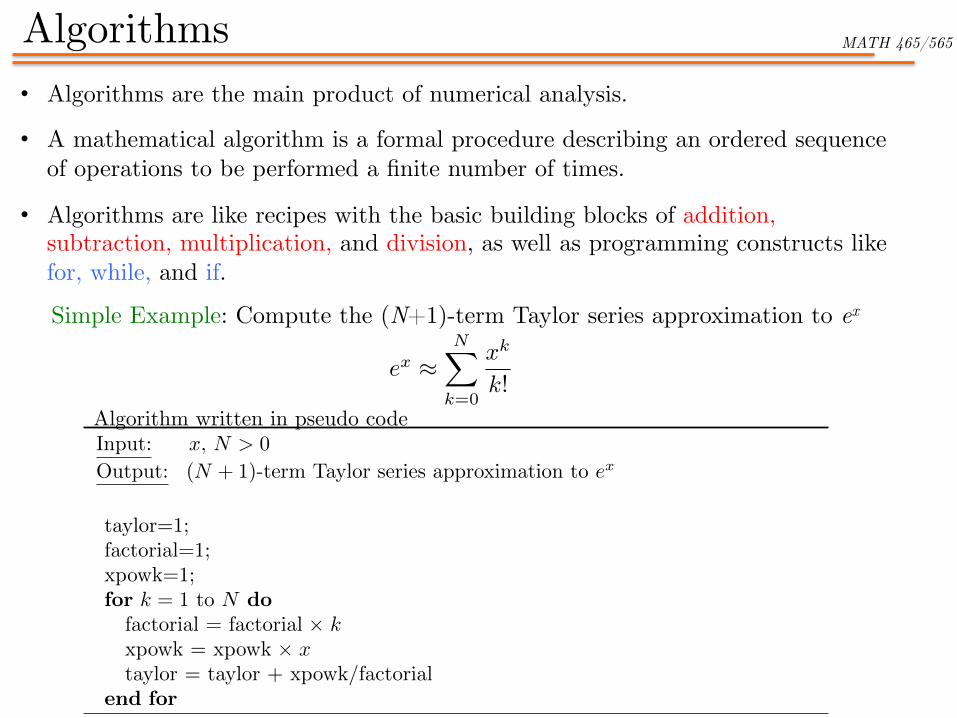
MATH 465/565 Algorithms •  Algorithms are the main product of numerical analysis.

•  A mathematical algorithm is a formal procedure describing an ordered sequence of operations to be performed a finite number of times.

•  Algorithms are like recipes with the basic building blocks of addition, subtraction, multiplication, and division, as well as programming constructs like for, while, and if.

Simple Example: Compute the (N+1)-term Taylor series approximation to ex

Algorithm written in pseudo code Input: x, N > 0

Output: (N + 1)-term Taylor series approximation to e

x

taylor=1;factorial=1;xpowk=1;for k = 1 to N do

factorial = factorial ⇥ k

xpowk = xpowk ⇥ x

taylor = taylor + xpowk/factorialend for

e

x ⇡NX

k=0

x

k

k!

MATH 465/565 Algorithms

•  Three primary concerns for algorithms:

§  Accuracy: How good is the algorithm at approximating the underlying quantity.

§  Stability: Is the output of the algorithm sensitive to small changes in the input data.

§  Efficiency: How much time does it take the algorithm to obtain a reasonable approximation.

•  We will discuss these for the algorithms considered in this course.

•  Some other important concerns include robustness, storage, and parallelization. o  These will be considered to a lesser extent

MATH 465/565 Algorithms •  Algorithms can be classified into two types:

§  Direct methods: Obtain the solution in a finite number of steps, assuming no rounding errors. Example: Solving a linear system with Gaussian elimination

§  Iterative methods: Generate a sequence of approximation that converge to the solution as the number of steps approaches infinity. Example:

MATH 465/565 Errors

•  Major sources of errors in numerical analysis:

§  Truncation errors: Result from the premature termination of an infinite computation. Example:

These are the primary concern of computational math.

§  Round-off errors: Result from using floating point arithmetic. Less significant than truncation errors, but nevertheless can result in catastrophic problems (see course webpage for examples).

•  Other errors that must be accounted for: Human errors, modeling errors, and measurement errors.

MATH 465/565 Measuring errors •  This course is about approximation. How do we measure errors in these

approximations? •  Let p be an approximation to p*, then we have two ways of measuring the

error:

§  Absolute error:

§  Relative error:

•  Relative error is typically the best, but it depends on the problem.

•  To illustrate this point consider the following simple example Example:

What are the absolute and relative errors in these cases? Which value makes the most sense to use?

MATH 465/565 Example of truncation and round-off error

f

0(x0) ⇡f(x0 + h)� f(x0)

h

•  Simple approximation of the derivative of a function:

As h �! 0 the approximation should get better and better.

10-20 10-15 10-10 10-5 100�

10-1610-14

10-1210-1010-8

10-610-4

10-2100

����

����

��

•  Example:

f(x) = sin(x), x0 = ⇡/4

����f0(x0)�

f(x0 + h)� f(x0)

h

����

Theoretical truncation error

Round-o↵ error

MATH 465/565 Convergence •  Some algorithms result in a sequence of approximations.

•  We often want to know if these sequences converge and how fast. •  Convergence/divergence:

•  Example:

MATH 465/565 Convergence rate and order •  We measure the speed of convergence of a sequence by the rate of convergence or

the order of convergence.

•  Big-O notation for understanding asymptotic behavior of functions and sequences:

•  Definition: Rate of convergence

•  Example:

Let pn =

1

n2� 2

n3+

5

n7and �n =

1

n2. Then {pn} converges to p = 0

as n ! 1 with a rate of convergence

1

n2, or pn = O

✓1

n2

◆.

Suppose lim

n!1pn = p and pn = O(�n) with lim

n!1�n = p. Then {pn}

is said to converge to p with rate of convergence �n.

• We say f(x) = O(g(x)) as x ! 1 if there exists a constant M > 0 such

that |f(x)| M |g(x)| for all x � x0.

• We say an = O(bn) as n ! 1 if there exists a constant C > 0 such that

|an| C|bn| for all n � N .

• We say e(h) = O(hq) as h ! 0 if there exists positive constants q and C

such that |e(h)| Chq

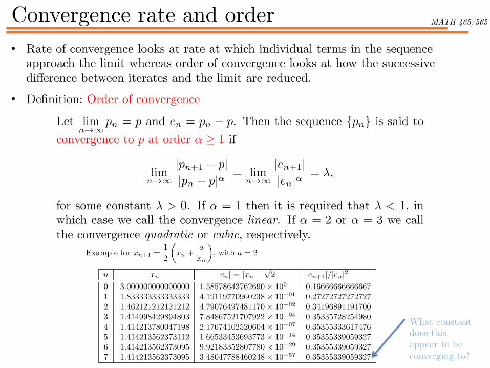
MATH 465/565 Convergence rate and order •  Rate of convergence looks at rate at which individual terms in the sequence

approach the limit whereas order of convergence looks at how the successive difference between iterates and the limit are reduced.

•  Definition: Order of convergence

What constant does this appear to be converging to?

MATH 465/565 Useful theorems from calculus