2015 1990 1 module 7: construction of indicators tools for civil society to understand and use...
TRANSCRIPT

12015
1990 Module 7: Module 7:
Construction of IndicatorsConstruction of Indicators
Tools for Civil Society to Understand Tools for Civil Society to Understand and Use Development Data: and Use Development Data:
Improving MDG Policymaking and Improving MDG Policymaking and MonitoringMonitoring

22015
1990
What you will be able to do by What you will be able to do by the end of this module:the end of this module:
• Understand the major types of quantitative Understand the major types of quantitative indicators, and how they are formulatedindicators, and how they are formulated
• Understand the role that a measure of variation Understand the role that a measure of variation plays in using and interpreting indicatorsplays in using and interpreting indicators

32015
1990
Quantitative Indicators: Quantitative Indicators: FormulationFormulation
• MeansMeans
• RatiosRatios
• ProportionsProportions
• PercentagesPercentages
• RatesRates
• QuantilesQuantiles
• Gini coefficientGini coefficient

42015
1990
MeansMeans
‘‘Average’ of two or more values:Average’ of two or more values:
• Simple: Sum of values/number of valuesSimple: Sum of values/number of values
• Weighted: Multiply values by some weighting Weighted: Multiply values by some weighting factor before summing, then divide by the sum of factor before summing, then divide by the sum of weightsweights
patients ofnumber
patients allby waited timesall of sumclinic aat time waitingAverage

52015
1990
Price increasePrice increase
% of price % of price increaseincrease
Income spentIncome spent % of income % of income spentspent
MeatMeat 1212 10001000 5050
BreadBread 2020 800800 4040
FruitFruit 120120 200200 1010
Food averageFood average ?????? 20002000 100100

62015
1990
Price increase (2)Price increase (2)
% of price % of price increaseincrease
Income spentIncome spent % of income % of income spentspent
MeatMeat 1212 10001000 5050
BreadBread 2020 800800 4040
FruitFruit 120120 200200 1010
Food averageFood average (12+20+120)/(12+20+120)/3=50.73=50.7
20002000 100100

72015
1990
Price increase (3)Price increase (3)
% of price % of price increaseincrease
Income Income spentspent
% of income % of income spentspent
MeatMeat 1212 10001000 5050
BreadBread 2020 800800 4040
FruitFruit 120120 200200 1010
Food averageFood average 1212∙∙50/10050/100+20+20∙∙
40/10040/100++120120∙∙1010/ / 100100=26=26
20002000 100100

82015
1990
RatiosRatios
• A ratio is the division of two numbers which A ratio is the division of two numbers which are both measured in the same unitsare both measured in the same units
- Compares like quantities- Compares like quantities
- Result has no units- Result has no units
• Example:Example:
- MDG I9: Ratio of girls to boys in primary, - MDG I9: Ratio of girls to boys in primary, secondary and tertiary educationsecondary and tertiary education

92015
1990
Ratios (2)Ratios (2)
Country, Country, yearyear
IndicatorIndicator GirlsGirls BoysBoys RatioRatio
Belarus, Belarus, 20062006
Net enrollment in Net enrollment in general secondary general secondary educationeducation
89.9689.96 87.0687.06 1.021.02
Moldova, Moldova, 20062006
Gross enrollment in Gross enrollment in general secondary general secondary educationeducation
83.6683.66 80.9280.92 1.031.03
Source: World Development Indicators, World Bank, 2008Source: World Development Indicators, World Bank, 2008

102015
1990
ProportionsProportions
When the ratio takes the form of a part divided by When the ratio takes the form of a part divided by the whole, it is called a proportionthe whole, it is called a proportion
Proportions therefore have no unitsProportions therefore have no units

112015
1990
Proportions (2)Proportions (2)
Example. Rural population as a proportion of total Example. Rural population as a proportion of total population, 2006population, 2006
CountryCountry Rural Rural population, population, thousand thousand peoplepeople
Total Total population, population, thousand thousand peoplepeople
ProportionProportion
BelarusBelarus 2658.92658.9 9732.59732.5 0.2730.273
MoldovaMoldova 2032.92032.9 3832.73832.7 0.5300.530
Source: World Development Indicators, World Bank, 2008Source: World Development Indicators, World Bank, 2008

122015
1990
PercentagesPercentages
To express a proportion as a percentage, multiply it To express a proportion as a percentage, multiply it by 100%by 100%
So, in 2006 in rural areas lived So, in 2006 in rural areas lived
0.273 0.273 ∙ 100%=27.3% and ∙ 100%=27.3% and
0.530 ∙ 100%=53.0% 0.530 ∙ 100%=53.0%
of the total population in Belarus and Moldova of the total population in Belarus and Moldova correspondinglycorrespondingly

132015
1990
RatesRates
When the numerator and denominator of a quotient When the numerator and denominator of a quotient do not have the same units, but are related in some do not have the same units, but are related in some other way, the result is a rateother way, the result is a rate
We usually use the word ‘per’ in the description of a We usually use the word ‘per’ in the description of a raterate
142015
1990
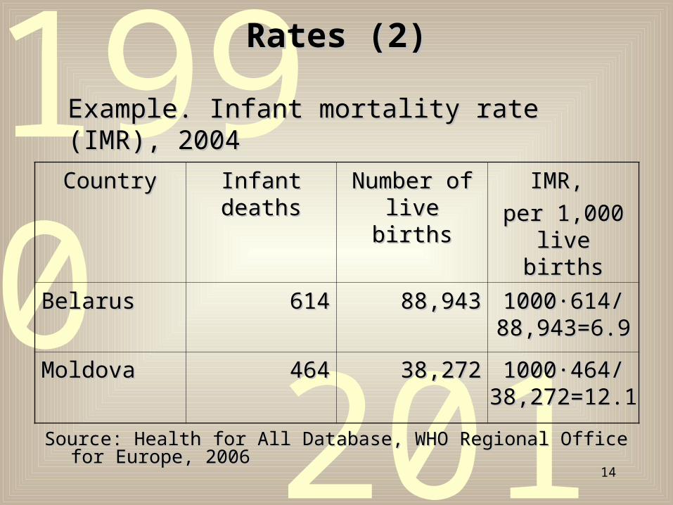
Rates (2)Rates (2)
Example. Infant mortality rate (IMR), 2004Example. Infant mortality rate (IMR), 2004
CountryCountry Infant deathsInfant deaths Number of Number of live live birthsbirths
IMR, IMR,
per 1,000 live per 1,000 live birthsbirths
BelarusBelarus 614614 88,94388,943 10001000∙614/ ∙614/ 88,943=88,943=6.96.9
MoldovaMoldova 464464 38,27238,272 10001000∙464/ ∙464/ 38,272=12.138,272=12.1
Source: Health for All Database, WHO Regional Office for Europe, 2006Source: Health for All Database, WHO Regional Office for Europe, 2006

152015
1990
Standardized RatesStandardized RatesExample. Crude (unweighted) and standardized Example. Crude (unweighted) and standardized
(weighted) death rates in urban and rural areas of (weighted) death rates in urban and rural areas of RomaniaRomania
Source: Mark Woodward, 2005, “Epidemiology: Study Design Source: Mark Woodward, 2005, “Epidemiology: Study Design and Data Analysis, 2nd ed.”, Chapman & Hall/CRC, Boca Ratonand Data Analysis, 2nd ed.”, Chapman & Hall/CRC, Boca Raton
PopulationPopulation DeathsDeathsAge groupAge group UrbanUrban RuralRural TotalTotal UrbanUrban RuralRural
0-90-9 18006801800680 13595011359501 31601813160181 35263526 49974997
10-1910-19 21281502128150 16429411642941 37710913771091 10101010 10491049
20-2920-29 19671101967110 14505501450550 34176603417660 15991599 19771977
30-3930-39 21182052118205 10190151019015 31372203137220 43334333 33003300
40-4940-49 16910331691033 11390651139065 28300982830098 83128312 69036903
50-5950-59 12004121200412 13960801396080 25964922596492 1489614896 1673916739
60-6960-69 921072921072 13807091380709 23017812301781 2419124191 3244332443
70-7970-79 404304404304 670133670133 10744371074437 2370623706 3887238872
80+80+ 175238175238 291062291062 466300466300 2590925909 4956149561
TotalTotal 1240620412406204 1034905610349056 2275526022755260 107482107482 155841155841

162015
1990
Standardized Rates (2)Standardized Rates (2)
Crude death rate, per 1,000 population (CDR) = Crude death rate, per 1,000 population (CDR) = =1000 =1000 ∙ ∙ total deaths / total populationtotal deaths / total population
Urban CDR = 1000 Urban CDR = 1000 ∙ ∙ (3526+1010 + …+ 25909)/ (3526+1010 + …+ 25909)/ 12406204 = 8.6612406204 = 8.66
Rural CDR = 1000 Rural CDR = 1000 ∙ ∙ (4997+1049 + … +49561)/ (4997+1049 + … +49561)/ 10349056 = 15.0610349056 = 15.06
Seems to be a large difference between urban and Seems to be a large difference between urban and rural CDRs, which could depend, however, on age rural CDRs, which could depend, however, on age structure of the populationstructure of the population

172015
1990
Standardized Rates (3)Standardized Rates (3)
Standardized death rate, per 1,000 population (SDR) Standardized death rate, per 1,000 population (SDR) ==
==
The weights used to calculate the SDR for both The weights used to calculate the SDR for both urban and rural areas must be the same and must be urban and rural areas must be the same and must be equal to the shares of each age group’s population in equal to the shares of each age group’s population in total populationtotal population
weightsof Sum
groups age year-ten for
rates death crude of sum Weighted

182015
1990
Standardized Rates (Standardized Rates (44))
• Age 0-9Age 0-9
- Urban CDR = 1000 - Urban CDR = 1000 ∙ ∙ 3526 / 1800680 = 1.963526 / 1800680 = 1.96
- Rural CDR = 1000 - Rural CDR = 1000 ∙ ∙ 4997 / 1359501 = 3.684997 / 1359501 = 3.68
- Weight = (1800680 + 1359501) / 22755260 = - Weight = (1800680 + 1359501) / 22755260 = 0.1390.139
• Age 10-19Age 10-19
- Urban CDR = 1000 - Urban CDR = 1000 ∙ 1010∙ 1010 / 2128150 = 0.47 / 2128150 = 0.47
- Rural CDR = 1000 - Rural CDR = 1000 ∙ 1049∙ 1049 / 1642941 = 0.64 / 1642941 = 0.64
- Weight = (2128150 + 1642941) / 22755260 = - Weight = (2128150 + 1642941) / 22755260 = 0.1660.166
• Etc.Etc.

192015
1990
Standardized Rates (Standardized Rates (55))
• Urban SDR = 1000 Urban SDR = 1000 ∙ (1.96∙ (1.96 ∙ 0.139 + 0.47∙ 0.139 + 0.47 ∙ 0.166 ∙ 0.166 + + … + 147.85+ + … + 147.85 ∙ 0.020) / 1∙ 0.020) / 1** = 11.24 = 11.24
• Rural SDR = 1000 Rural SDR = 1000 ∙ (3.68 ∙ 0.139 + 0.64 ∙ 0.166 + ∙ (3.68 ∙ 0.139 + 0.64 ∙ 0.166 + + … + 170.28 + … + 170.28 ∙ 0.020) / 1∙ 0.020) / 1** = 11.99 = 11.99
• Unlike crude death rates, there is only minor Unlike crude death rates, there is only minor difference in standardized death rates between difference in standardized death rates between urban and rural areasurban and rural areas
* 1 = Sum of weights* 1 = Sum of weights

202015
1990
QuantilesQuantiles• Quantiles are a set of points that, according to Quantiles are a set of points that, according to
their values, divide a set of ordered values into a their values, divide a set of ordered values into a defined number of groups each containing the defined number of groups each containing the same number of valuessame number of values
• E.g., three quantiles divide a set of numbers into E.g., three quantiles divide a set of numbers into four groupsfour groups
• The following quantiles are used often: median The following quantiles are used often: median (two groups), tertiles (three groups), quartiles (two groups), tertiles (three groups), quartiles (four groups), quintiles (five groups), deciles (ten (four groups), quintiles (five groups), deciles (ten groups), percentiles (one hundred groups)groups), percentiles (one hundred groups)
QQ11 QQ22 QQ33
212015
1990
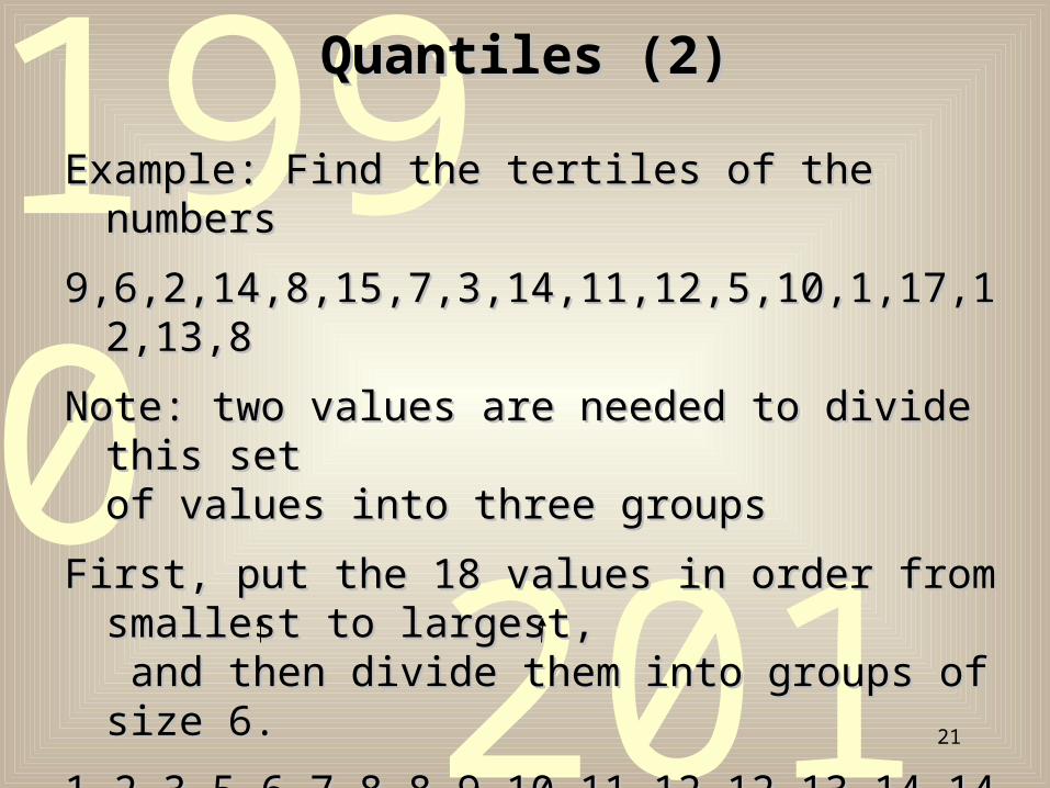
Quantiles (2)Quantiles (2)
Example: Find the tertiles of the numbersExample: Find the tertiles of the numbers
9,6,2,14,8,15,7,3,14,11,12,5,10,1,17,12,13,89,6,2,14,8,15,7,3,14,11,12,5,10,1,17,12,13,8
Note: two values are needed to divide this set Note: two values are needed to divide this set of values into three groupsof values into three groups
First, put the 18 values in order from smallest to First, put the 18 values in order from smallest to largest,largest, and then divide them into groups of size 6. and then divide them into groups of size 6.
1,2,3,5,6,7,8,8,9,10,11,12,12,13,14,14,15,171,2,3,5,6,7,8,8,9,10,11,12,12,13,14,14,15,17
tt11 t t22
Here, tHere, t11 = 7.5 and t = 7.5 and t22 = 12 = 12

222015
1990
Quantiles (3)Quantiles (3)
Example. Indicator for MDG1: Share of the Example. Indicator for MDG1: Share of the poorest quintile in national consumptionpoorest quintile in national consumption
• Estimate household consumption (from Estimate household consumption (from household survey data)household survey data)
• Adjust consumption for household size (to get per Adjust consumption for household size (to get per capita consumption); to determine per capita capita consumption); to determine per capita consumption, divide household consumption by consumption, divide household consumption by the (equivalent) number of people in the the (equivalent) number of people in the householdhousehold

232015
1990
Quantiles (4)Quantiles (4)
• Rank people by per capita consumption (smallest Rank people by per capita consumption (smallest to largest)to largest)
• Find the first quintile (QFind the first quintile (Q11))
• Aggregate all consumption less than QAggregate all consumption less than Q11, and , and aggregate all consumptionaggregate all consumption
• Divide the sum of all consumption below QDivide the sum of all consumption below Q11 by by the sum of all consumption the sum of all consumption
• This ratio multiplied by 100% is the value of MDG This ratio multiplied by 100% is the value of MDG indicatorindicator

242015
1990
Lorenz curve of income distribution
0%
10%
20%
30%
40%
50%
60%
70%
80%
90%
100%
0% 10% 20% 30% 40% 50% 60% 70% 80% 90% 100%
Cumulative population share
Cu
mu
lati
ve
in
co
me
sh
are
Gini CoefficientGini Coefficient
This is a special indicator used to measure inequalityThis is a special indicator used to measure inequality1 → complete inequality, 0 → complete equality1 → complete inequality, 0 → complete equality
Gini coefficient = Area A/(Area A + Area B)Gini coefficient = Area A/(Area A + Area B)
A
B
252015
1990
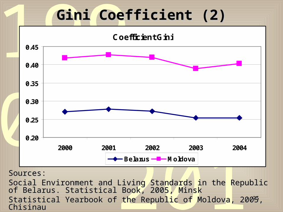
Gini Coefficient (2)Gini Coefficient (2)Coefficient Gini
0.20
0.25
0.30
0.35
0.40
0.45
2000 2001 2002 2003 2004
Belarus Moldova
Sources: Sources: Social Environment and Living Standards in the Republic of Belarus. Social Environment and Living Standards in the Republic of Belarus. Statistical Book, 2005, MinskStatistical Book, 2005, MinskStatistical Yearbook of the Republic of Moldova, 2005, ChisinauStatistical Yearbook of the Republic of Moldova, 2005, Chisinau

262015
1990
Indicators and VariabilityIndicators and Variability
An indicator such as a percentage or a quintile An indicator such as a percentage or a quintile gives a ‘snapshot’ picture of some particular aspect gives a ‘snapshot’ picture of some particular aspect of the process of the process it representsit represents
Example.Example. Per capita income in Kyrgyzstan by Per capita income in Kyrgyzstan by settlement type, thousand Kyrgyz somssettlement type, thousand Kyrgyz soms
Source: ADB Study on Source: ADB Study on Remittances and PovertyRemittances and Poverty in Central Asia and in Central Asia and Caucasus, 2007Caucasus, 2007
38.0
22.519.7
capital city other urban rural

272015
1990
Indicators and Variability (2)Indicators and Variability (2)
• Looks like income per capita is higher in capital Looks like income per capita is higher in capital city than in two other types of settlements, and in city than in two other types of settlements, and in other towns it is higher than in rural areasother towns it is higher than in rural areas
• Need to be able to prove this, by using Need to be able to prove this, by using information about the standard error of the information about the standard error of the variable as evidencevariable as evidence

282015
1990
Indicators and Variability (3)Indicators and Variability (3)
• The estimated standard error is a measure of The estimated standard error is a measure of sampling error; usually the larger sample size the sampling error; usually the larger sample size the smaller this errorsmaller this error
• In fact, we usually prefer to convert this into a In fact, we usually prefer to convert this into a range of values within which we expect to find the range of values within which we expect to find the estimateestimate
• We describe the likelihood of the range containing We describe the likelihood of the range containing the estimate with a percentage – usually 95%the estimate with a percentage – usually 95%

292015
1990
Indicators and Variability (4)Indicators and Variability (4)
• With probability 95% it is possible to claim that With probability 95% it is possible to claim that per capita income in the capital city is higher than per capita income in the capital city is higher than in other settlementsin other settlements
• But, with 5% error probability it is impossible to But, with 5% error probability it is impossible to claim that there is a difference in per capita claim that there is a difference in per capita income between other urban and rural areasincome between other urban and rural areas
95% confidence intervals for per capita income
15
25
35
45
capital city other urban rural
Th
ou
san
d K
yrg
yz s
om
s

302015
1990
Indicators and Variability (5)Indicators and Variability (5)Maternal mortality estimates, Maternal mortality estimates,
with confidence intervalswith confidence intervals
Source: UNICEFSource: UNICEF
0
2 0 0
4 0 0
6 0 0
8 0 0
1 0 0 0
1 2 0 0
1 4 0 0
A fr ic a A s ia L a t inA m e r ic a /
C a r ib b e a n
D e v e lo p e d W o r ld
L o w e s t im a te P o in t e s t im a te U p p e r e s t im a te

312015
1990
SummarySummary
• We have looked at the major types of quantitative We have looked at the major types of quantitative indicators in terms ofindicators in terms of
- Formulation- Formulation
- Characteristics- Characteristics
- Uses- Uses
- Interpretation- Interpretation• We have discussed the role that variability We have discussed the role that variability
and measures of it can play in enhancing the and measures of it can play in enhancing the interpretation and use of indicatorsinterpretation and use of indicators

322015
1990
Practical 7Practical 7
1.1. Why are quantiles useful as indicators of national Why are quantiles useful as indicators of national
and sub-national development?and sub-national development?
2.2. Why use rates as indicators rather than actual Why use rates as indicators rather than actual numbers?numbers?
3.3. Why is standardization useful for comparing the Why is standardization useful for comparing the situation between sub-populations? situation between sub-populations?

332015
1990
Practical 7 (2)Practical 7 (2)
4.4. Look at the following examples, and say whether Look at the following examples, and say whether a real difference exists:a real difference exists:
• Ratio of girls to boys in secondary school:Ratio of girls to boys in secondary school:
1995: 0.94 95% confidence interval (0.93, 0.95) 1995: 0.94 95% confidence interval (0.93, 0.95)
2000: 0.95 95% confidence interval (0.88, 1.02)2000: 0.95 95% confidence interval (0.88, 1.02)• Population below the food poverty line: Population below the food poverty line:
1991/92: 21.6%1991/92: 21.6% 95% confidence interval (20.5, 22.7) 95% confidence interval (20.5, 22.7)
2000/01: 18.7%2000/01: 18.7% 95% confidence interval (17.7, 19.7) 95% confidence interval (17.7, 19.7) • The following sequence of infant mortality rates: The following sequence of infant mortality rates:
Year Infant Mortality RateYear Infant Mortality Rate
19901990 3030
1994 1994 2828
1997 1997 2222
2000 2000 2121
2003 2003 1818