Contents

1 Introduction 11.1 Need of the project: . . . . . . . . . . . . . . . . . . . . . . . . . . . . . . . . 11.2 26/7: What went wrong? Why the need for a area-wise prediction system? . 21.3 Scope of the Project: . . . . . . . . . . . . . . . . . . . . . . . . . . . . . . . 6

2 Literature Survey 72.1 Monitoring Rain Rate with Data from Networks of Microwave Transmission

Links - Christian Mtzler, Ernest Koffi and Alexis Berne . . . . . . . . . . . . 72.2 Cumulative distributions of rainfall rate and microwave attenuation in Singa-

pore’s tropical region - Z. X. Zhou, L. W. Li, T. S. Yeo, and M. S. Leong . . 82.2.1 Comparisons of experimental and CCIR predictions . . . . . . . . . . 9

2.3 Rain Attenuation Measurements in Amritsar over terrestrial microwave linkat 19.4 & 28.75 GHz - Ashok Kumar, I. S. Hudiara, Sarita Sharma And VibhuSharma . . . . . . . . . . . . . . . . . . . . . . . . . . . . . . . . . . . . . . 10

2.4 Monitoring of rainfall by ground-based passive microwave systems:Models,measurements and applications - F. S. Marzano, D. Cimini, and R. Ware . . 11

2.5 Rain Attenuation Modeling In The 10-100 GHz Frequency Using Drop SizeDistributions For Different Climatic Zones In Tropical India - S. Das, A.Maitra, A. K. Shukla . . . . . . . . . . . . . . . . . . . . . . . . . . . . . . . 13

2.6 Inference . . . . . . . . . . . . . . . . . . . . . . . . . . . . . . . . . . . . . . 14

3 Basics of Rainfall Measurements 153.1 Rain Fall Intensity: . . . . . . . . . . . . . . . . . . . . . . . . . . . . . . . . 153.2 Rainfall Recording . . . . . . . . . . . . . . . . . . . . . . . . . . . . . . . . 15

3.2.1 Non-recording Gauges . . . . . . . . . . . . . . . . . . . . . . . . . . 153.2.2 Automatic Recording Gauges . . . . . . . . . . . . . . . . . . . . . . 16

3.3 Duration of Rainfall . . . . . . . . . . . . . . . . . . . . . . . . . . . . . . . 183.4 Frequency of Rainfall . . . . . . . . . . . . . . . . . . . . . . . . . . . . . . . 183.5 The Watershed Concept . . . . . . . . . . . . . . . . . . . . . . . . . . . . . 18

3.5.1 A watershed is a precipitation collector . . . . . . . . . . . . . . . . . 193.5.2 Not all precipitation that falls in a watershed flows out . . . . . . . . 19

4 Rain Attenuation and Now-casting 214.1 Microwave attenuation to predict rain-rate . . . . . . . . . . . . . . . . . . . 214.2 Need of Now-casting . . . . . . . . . . . . . . . . . . . . . . . . . . . . . . . 224.3 Parameters that contribute to floods . . . . . . . . . . . . . . . . . . . . . . 24

4.3.1 Infiltration: . . . . . . . . . . . . . . . . . . . . . . . . . . . . . . . . 244.3.2 Soil Characteristics: . . . . . . . . . . . . . . . . . . . . . . . . . . . . 24

i

4.3.3 Plants and Animals: . . . . . . . . . . . . . . . . . . . . . . . . . . . 254.3.4 Slopes . . . . . . . . . . . . . . . . . . . . . . . . . . . . . . . . . . . 264.3.5 Runoff and Flooding . . . . . . . . . . . . . . . . . . . . . . . . . . . 264.3.6 Runoff and Urban Development . . . . . . . . . . . . . . . . . . . . . 264.3.7 Drainage system . . . . . . . . . . . . . . . . . . . . . . . . . . . . . 274.3.8 Tides . . . . . . . . . . . . . . . . . . . . . . . . . . . . . . . . . . . . 27

5 Flood Prediction System 285.1 Defining the topography: . . . . . . . . . . . . . . . . . . . . . . . . . . . . . 285.2 Creating a grid of recorded data: . . . . . . . . . . . . . . . . . . . . . . . . 285.3 Finding the number of sinks: . . . . . . . . . . . . . . . . . . . . . . . . . . . 295.4 Finding the watershed . . . . . . . . . . . . . . . . . . . . . . . . . . . . . . 305.5 Flooding . . . . . . . . . . . . . . . . . . . . . . . . . . . . . . . . . . . . . . 31

6 Experimentation and Result Analysis 32

7 Comparison of Rain Attenuation Models 387.1 ITU-R Model . . . . . . . . . . . . . . . . . . . . . . . . . . . . . . . . . . . 387.2 The Indian Model . . . . . . . . . . . . . . . . . . . . . . . . . . . . . . . . . 397.3 Simple Attenuation Model . . . . . . . . . . . . . . . . . . . . . . . . . . . . 407.4 Crane Model . . . . . . . . . . . . . . . . . . . . . . . . . . . . . . . . . . . 427.5 Earth to Space Model . . . . . . . . . . . . . . . . . . . . . . . . . . . . . . 437.6 Tropical Model . . . . . . . . . . . . . . . . . . . . . . . . . . . . . . . . . . 46

8 Conclusion and Future Work 498.1 Conclusion . . . . . . . . . . . . . . . . . . . . . . . . . . . . . . . . . . . . . 498.2 Future Work . . . . . . . . . . . . . . . . . . . . . . . . . . . . . . . . . . . . 49

References 508.3 Reference Papers . . . . . . . . . . . . . . . . . . . . . . . . . . . . . . . . . 50

ii

List of Figures

1.1 Rainfall in different areas of Mumbai on July 26 . . . . . . . . . . . . . . . . 21.2 Percentage of days with rainfall above a given threshold along the western coast 41.3 Fig 1:History of heavy rainfall days in Mumbai . . . . . . . . . . . . . . . . . 51.4 Extraordinarily heavy rainfall events over India . . . . . . . . . . . . . . . . 6

2.1 Extinction coefficient A in dB/km at 38 GHz of rain at a temperature T=283Kversus rain rate R in mm/h for the four drop-size distributions . . . . . . . . 8

2.2 Cumulative distribution of rainfall rate in Singapore compared with the In-ternational Radio Consultative Committee (CCIR) prediction . . . . . . . . 9

2.3 Relationship between attenuation and rainfall rate compared with that of theCCIR at frequencies of 15 and 38.6 GHz. . . . . . . . . . . . . . . . . . . . . 10

2.4 The measured and ITU-R rain rate . . . . . . . . . . . . . . . . . . . . . . . 112.5 Annual cumulative percentage of time for path attenuation exceeding present

level . . . . . . . . . . . . . . . . . . . . . . . . . . . . . . . . . . . . . . . . 112.6 Annual cumulative percentage of time for path attenuation exceeding preset

level . . . . . . . . . . . . . . . . . . . . . . . . . . . . . . . . . . . . . . . . 122.7 Specific attenuation for different locations with frequency a rain rate (a) 10

mm/h, (b) 25 mm/h, (c) 50mm/h and (d) 100 mm/h. . . . . . . . . . . . . . 14

3.1 Watershed . . . . . . . . . . . . . . . . . . . . . . . . . . . . . . . . . . . . . 18

5.1 Watershed Topography categorized according to their averaged heights . . . 295.2 The direction in which the water from a particular cell will flow . . . . . . . 295.3 Watershed table . . . . . . . . . . . . . . . . . . . . . . . . . . . . . . . . . . 305.4 Watershed connected by their spill heights . . . . . . . . . . . . . . . . . . . 30

6.1 Elevation Grid . . . . . . . . . . . . . . . . . . . . . . . . . . . . . . . . . . . 326.2 Watershed Map . . . . . . . . . . . . . . . . . . . . . . . . . . . . . . . . . . 336.3 Watershed Graph . . . . . . . . . . . . . . . . . . . . . . . . . . . . . . . . . 346.4 The plot shows the region prior to the beginning of the simulation. . . . . . 356.5 The plot shows the region after the simulation began. . . . . . . . . . . . . . 356.6 The plot shows the area getting flooded (marked in red) . . . . . . . . . . . 366.7 The plot shows different regions getting flooded (marked in red) . . . . . . . 366.8 This plot gives the time duration in which the individual regions (watersheds)

flooded over. Also the time required for the region on interest to flood isdisplayed along with the name of the area which that watershed represents. . 37

7.1 The ITU-R model . . . . . . . . . . . . . . . . . . . . . . . . . . . . . . . . . 397.2 The Indian rain attenuation prediction model . . . . . . . . . . . . . . . . . 40

iii

7.3 The Simple attenuation model . . . . . . . . . . . . . . . . . . . . . . . . . . 417.4 The Crane model . . . . . . . . . . . . . . . . . . . . . . . . . . . . . . . . . 437.5 The Earth to Space Improved Model . . . . . . . . . . . . . . . . . . . . . . 457.6 k and a for different regions are given at different frequencies . . . . . . . . . 47

iv

Rain Rate Monitoring and Flood Prediction Model

Project Report 2010 - 2011

by

Anjana IyerRhucha ParanjapeHemangi Sahare

Chaitali Walavalkar

under the guidance of

Prof. K. T. Talele

Department of Electronics & Telecommunication EngineeringSardar Patel Institute of Technology,

Munshi Nagar, Andheri (W), Mumbai - 400 058

April - 2011

acknowledgements

We feel privileged to thank our project guide, Prof. K. T. Talele for providing all thesupport needed for successful completion of the project. We would like to express our grati-tude towards his constant encouragement, and guidance throughout the development of theproject. We are indebted to the Indian Meteorological Department (IMD), Mumbai Divisionfor their persistent help and support. We would like to thank Arunkumar Mahadevan forhis innovative insights and help at various problems faced during the project.

We also thank Sardar Patel Institute of Technology for providing continuous access tothe required infrastructure. We would like to thank our fellow colleagues for their supportthroughout the project.

1

Abstract

The project involves monitoring of rain-rate from the degree of corresponding microwaveattenuation, followed by prediction of time taken for a particular region to flood, given aparticular rain-rate. The rain-rate measurement from microwave attenuation has been aknown potential for many years. A comparison of several rain attenuation models has beendemonstrated in detail. The rain-rate obtained from these relations is then integrated in amodel which also takes in account the topography to predict the time required for the regionto get flooded. The scope of the project is those cities which experience heavy rainfall andin turn suffer loss of life and property due to such rain floods. With this technique, it ispossible to predict a impending flood. Also this method of prediction can be applied to anyregion, provided the necessary data is available.

Project Objective

The city of Mumbai experienced the worst floods in history on 26th July 2005 when itrained about 994 mm in 24 hours. Loss of life and property because of floods has now becomea major issue. Hence it is necessary to monitor the rainfall in real time and consequentlyrelay appropriate warnings in case of such events. However, there is no system in place atpresent which can perform these tasks. Thus, the objective of our project is to achieve thesetasks.

The rain rate is monitored continuously with the help of corresponding microwave atten-uation. This rain-rate thus calculated is used as one of the input parameters in a floodprediction model based on the concept of watersheds. In addition, the topography of a re-gion also plays a crucial role in the time required for the region to get flooded. The systemis faster and thus reduces the time required to relay warnings during rain floods and henceprevent significant damages.

The current prediction technique involves satellite imagery and traditional rain gauges.With the proposed technique, it is possible to monitor rain-rate in real time and reduce theprediction time. The prime objective therefore is to provide an additional aid to the IndianMeteorological Department. The system could be integrated with the existing techniques offlood prediction. Also the key users could include civil agencies at national, provincial/stateand local level; military organization, corporations especially those which operate structures;voluntary emergency response organizations and the media.

Chapter 1

Introduction

Flooding is simultaneously one of nature’s most destructive and violent forces. Floodsoccur when the flow of water exceeds the amount that can be contained in a river’s naturalbanks or soil. This can happen due to a variety of factors, including rainfall intensity,duration, surface conditions, and the topography and slope of the receiving basin. Thedestructiveness of floods can also be exacerbated by many human activities, such as removingtrees and vegetation, modifying the course of rivers and streams, and development in floodplain and urban areas. Such floods are a common phenomenon in many regions of theworld and also a major form of natural disaster in many parts of the world. In the UnitedStates, where flood mitigation and prediction is advanced, floods do about $6 billion worthof damage and kill about 140 people every year. A 2007 report by the Organization forEconomic Cooperation and Development found that coastal flooding alone does some $3trillion in damage worldwide.

1.1 Need of the project:

The classical form of rain-related flood prediction involves use of traditional rain-gaugesspread over a large area in addition to the satellite imagery and meteorological radars Thedensity of rain gauges is not sufficient to cover whole area under consideration. Moreover theradars or other means used give only a synoptic view of the situation. Also the time takenfor processing such information and hence relaying suitable warnings is too large. Henceneed for a system that performs faster and has a shorter response time is crucial.

The rain gauges used at Indian Meteorological Department (IMD) are non-recording ones.The quantity of rainfall is measured every three hours. The data from these rain gaugesis then utilized for further analysis purposes. Based on these measurements, the averagerainfall of the day is calculated and recorded. This data along with cloud density fromsatellite imaging is used for weather forecasting. Non-recording rain gauges however giveaverage intensity of rainfall and not the actual rainfall intensity. They record data only inthree-hourly basis. The self recording ones are not automated to transmit in real time. Inessence, the real time data is not available. Data has to be retrieved and scrutinized before itcan be used in analysis. Hence after measurement of data, the result can be made availableonly after a couple of hours. Such a large window makes it difficult to predict the rainfallaccurately. The IMD uses synoptic scale models for most of it predictions while certainconcentrated rain events require meso-scale predictions.

1

1.2 26/7: What went wrong? Why the need for a area-

wise prediction system?

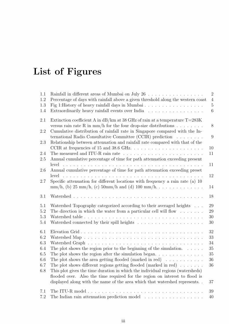
According to the IMD’s terminology for the classification of rainfall intensity, ”Rather HeavyRain” stands for 3.5 cm to 7.49 cm of rain over a 24 hour period, ”Heavy Rain” for 7.5 cmto 12.49 cm and ”Very Heavy Rain” for rain in excess of 12.5 cm. Clearly, the terminologyis grossly inadequate to classify the unprecedented rain of July 26 in Mumbai. The mete-orological station at Santacruz in North Mumbai recorded a whopping 94.4 cm of rain in24 hours. Some pockets seem to have received even higher rainfall (Table 1). But, giventhe relative frequencies of rainfall with different intensity during the monsoon period, theterminology is not without logic. Table 2, for example, shows the relative frequencies fordifferent rainfall intensity along the West Coast, where one witnesses spells of heavy rainfallduring the monsoon.

Figure 1.1: Rainfall in different areas of Mumbai on July 26

Historically, in more than a century of rainfall records of the IMD, the number of occasionsMumbai received more than 20 cm of rainfall in a day is 50; and, the number of occasionswith more than 30 cm is only 13 (Table 3). The highest previously recorded day’s rainfallin Mumbai is 57.56 cm on July 4, 1974. In fact, the July 26 rain in Mumbai was truly ex-traordinary even when compared with heaviest rainfall recorded in places such as Cherapunji(Table 4). But pertinently, in Mumbai’s case the rainfall (and hence the scale of the weathersystem that caused it) was extremely localized. The station at Colaba in the southern endof Mumbai recorded only 7.34 cm of rain on the same day.

2

The extraordinary precipitation seems to have been spread across 20 to 30 km only. Inmeteorological parlance, processes that extend over such small scales (20 km to 200 km)are known as ”mesoscale phenomena”, as against ”synoptic scale phenomena” (200 km to2,000 km), on which the routine observational meteorology is based. Usually, ”mesoscalephenomena” last for a very short duration (a few hours) while ”synoptic scale phenomena”can last for a couple of days.

Given the available synoptic and modeling techniques, forecasting such a rare and extreme,and that too highly localized, event would seem to be nearly impossible. The techniques ofsynoptic or short range, forecasting (one to three days ahead) are based on the knowledgeof events that occur with relatively high frequency. As Harold Brooks of the United States’National Oceanic and Atmospheric Administration (NOAA) points out: ”Essentially, we’relooking for ingredients to come together to produce such an extreme event and, in this case,they are unlikely to have been observed often enough to learn from them. We might be ableto predict a very heavy (about 30 cm) event, but not the incredible event that occurred.”

Even numerical weather prediction models require input data at appropriate spatial res-olution (grid points) to be fed into the model as initial conditions. Roughly speaking, toanalyze a complete wave of atmospheric disturbance any numerical model would requireat least data at five grid points. Hence if the intrinsic resolution of a numerical weatherprediction model is, say, 30 km (which would be a good model), the scale at which it canpossibly predict processes or the formation of weather systems would be 120 km. Even forvery high-resolution mesoscale forecasting models (say 5 km to 10 km resolution), it wouldbe a tough ask to predict a phenomena on such a small scale as across 20 km.

In fact, given the meteorological systems that were developing in the days prior to theevent, most models did predict heavy precipitation. But no model, at any forecasting centreof the world, could predict the extremely intense precipitation that occurred. Both theIMD, in its 24-hour forecast using a limited-area regional model, and the National Centre forMedium Range Weather Forecasting (NCMRWF), in its 48-hour forecast using a mesoscalemodel (with a 38 km resolution), had predicted 8cm to 16 cm of rain over Mumbai up to8-30 a.m. of July 27.

Some models around the world, like the one at the United Kingdom Meteorological Office,apparently forecast up to 30 cm of rain. Even this, as the frequencies of intense rainfallevents show, is of garden variety, and not anything unusual. However, according to AkhileshGupta of the NCMRWF, in a re-run of its model, with some improved input data assimila-tion techniques and changed input parameters (whose details are not known yet), the U.K.Meteorological Office found that its model predicted rainfall up to 80 cm. Notwithstandingthis, it would be fair to say at this point of time that, given the paucity of wind and pre-cipitation rate data, even the cause of the event (which is unlike any other in the past) ispuzzling to say the least, though some speculations have been made.

Considering that the event was not amenable to prediction, the question that naturallyarises is whether the people of Mumbai could have been forewarned, say a few hours ahead,of the impending disaster. For instance, the first warning, based on the local forecast for

3

Mumbai and suburbs, that the IMD sent out to all the agencies concerned on July 26, first at1-00 p.m. and repeated thereafter, said: ”Rather heavy to heavy rain accompanied by stronggusty winds likely in city and suburbs. Heavy rainfall likely to occur at a few places withvery heavy rainfall at isolated places over Konkanpatti-Goa during next 48 hours. Heavy tovery heavy rainfall likely to occur at isolated places over madhya [central] Maharashtra andMarathwada during the same period.”

Given the classification of the intensity of rainfall, this warning hardly conveys the gravityof the developing situation. But with the observed rainfall at that time (about 1 cm ofcumulative rain) and the limited instrumentation that is in place in the region, such awarning would seem natural and would have been considered appropriate by the IMD aswell.

Figure 1.2: Percentage of days with rainfall above a given threshold along the western coast

The instrumentation for weather-related measurements in Mumbai include manually op-erated rain gauges at variously located stations, whose data are recorded every three hoursand transmitted, two continuous self-recording rain gauges at Colaba and Santacruz mete-orological stations, and an X-band weather radar. The radar is basically a wind-and-stormdetection instrument which can, at best, be used to detect cloudiness and measure size anddepth of clouds.

If an S-band Doppler weather radar or radars (with a range of about 300 km) had been inplace, one would have got wind speeds of the rapid convection systems that were continuouslyfeeding high levels of moisture into the clouds in a localized fashion and the high precipitationrates. Such a radar would have been able to show not only how much rain had fallen and the

4

rate at which it had fallen, but also the extent of rain that was approaching the area hoursahead. However, while any such system would have probably warned of a rainfall intensityof 30 cm to 50 cm, a rainfall intensity of above 90 cm could not have been anticipated at allgiven the history of intense rainfall events in the region. But the event has certainly broughthome the urgency to implement the proposed Doppler Weather Radar (DWR) network alongcoastal India. It would also perhaps call for a rethink on the density of the network alongthe western coast. Unlike the network on the east for cyclone detection, a fewer numberhave been proposed along the west.

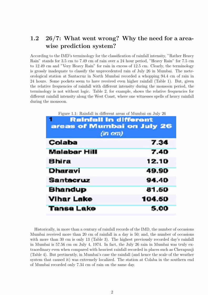
There was a rapid increase in the rate of precipitation at the Santacruz meteorologicalstation. In the three-hour duration between 2-30 p.m. and 5-30 p.m. on July 26, it pourednearly 39 cm; more rain per hour than a full day’s rain in many intense rainfall days duringmonsoon. Unfortunately, the instrumentation network of the IMD that is in place does notprovide real-time data online. While the manually operated rain gauges give data only inthree-hourly bins, the self-recording ones are not automated to transmit in real-time. Thedata has to be retrieved and scrutinized before it can be used in analysis.

Figure 1.3: Fig 1:History of heavy rainfall days in Mumbai

However, given the intense rainfall along Goa and coastal Karnataka in the preceding days,and given the sudden cloudburst-like activity in Mumbai, the meteorological officials shouldhave responded to the situation better and obtained the rain gauge data more frequently,say on a half-hourly or hourly basis. The first half-hour in the beginning of the next three-hourly bin (2-30 p.m. to 5-30 p.m.) itself would have indicated the extreme nature of theevent. That would have probably sufficed to issue an immediate red alert following theearlier warning. But this was not done and a couple of crucial hours were perhaps lost. Infact, the sad part is that till date, data from the continuous self-recording rain gauges arenot available even to the IMD headquarters in Delhi for a proper diagnosis of the event bothby the IMD and other researchers across the country.

5

Figure 1.4: Extraordinarily heavy rainfall events over India

1.3 Scope of the Project:

The purpose of the project is to put forth an efficient system for predicting floods. The basicprediction is based on forecasting the time required for a particular region to flood based onits topography and the corresponding rain-rate. In addition the use of microwave attenuationto predict the corresponding rain-rate has been proposed. There exists a relation betweenmicrowave attenuation and rain-rate proposed by the ITU-R. However some observationshave shown that this relation does not clearly define the conditions prevailing in the tropicalregions. In addition an analysis was done for the same by the mobile service provider Orangein the year 2010 .The project provides a detailed analysis of these relations and some relatedobservation.

The core model takes two primary inputs namely: rain-rate and topography of an area.For the purpose of the analysis a small region consisting of the Andheri, Vile Parle andJogeshwari areas in Mumbai. It forecasts the time required for a particular area to floodtaking into account the basic consideration that low-lying areas get flooded faster than thoserelatively higher than the sea-level. The flood prediction should take into account a widerange of factors such as the soil characteristics, the nature of soil et cetera. However theeffects of these parameters have not been accounted for due to lack of sufficient data.

The model provides satisfactory results for flood prediction and can be expanded to includemore parameters and give more accurate results. With the inclusion of a variety of factorsand parameters an elaborate flood prediction system can be designed.

6

Chapter 2

Literature Survey

This chapter includes the summary of all the papers referred and studied for the imple-mentation of the project.

2.1 Monitoring Rain Rate with Data from Networks of

Microwave Transmission Links - Christian Mtzler,

Ernest Koffi and Alexis Berne

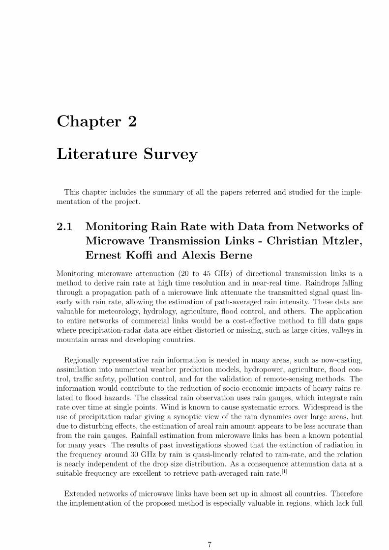
Monitoring microwave attenuation (20 to 45 GHz) of directional transmission links is amethod to derive rain rate at high time resolution and in near-real time. Raindrops fallingthrough a propagation path of a microwave link attenuate the transmitted signal quasi lin-early with rain rate, allowing the estimation of path-averaged rain intensity. These data arevaluable for meteorology, hydrology, agriculture, flood control, and others. The applicationto entire networks of commercial links would be a cost-effective method to fill data gapswhere precipitation-radar data are either distorted or missing, such as large cities, valleys inmountain areas and developing countries.

Regionally representative rain information is needed in many areas, such as now-casting,assimilation into numerical weather prediction models, hydropower, agriculture, flood con-trol, traffic safety, pollution control, and for the validation of remote-sensing methods. Theinformation would contribute to the reduction of socio-economic impacts of heavy rains re-lated to flood hazards. The classical rain observation uses rain gauges, which integrate rainrate over time at single points. Wind is known to cause systematic errors. Widespread is theuse of precipitation radar giving a synoptic view of the rain dynamics over large areas, butdue to disturbing effects, the estimation of areal rain amount appears to be less accurate thanfrom the rain gauges. Rainfall estimation from microwave links has been a known potentialfor many years. The results of past investigations showed that the extinction of radiation inthe frequency around 30 GHz by rain is quasi-linearly related to rain-rate, and the relationis nearly independent of the drop size distribution. As a consequence attenuation data at asuitable frequency are excellent to retrieve path-averaged rain rate.[1]

Extended networks of microwave links have been set up in almost all countries. Thereforethe implementation of the proposed method is especially valuable in regions, which lack full

7

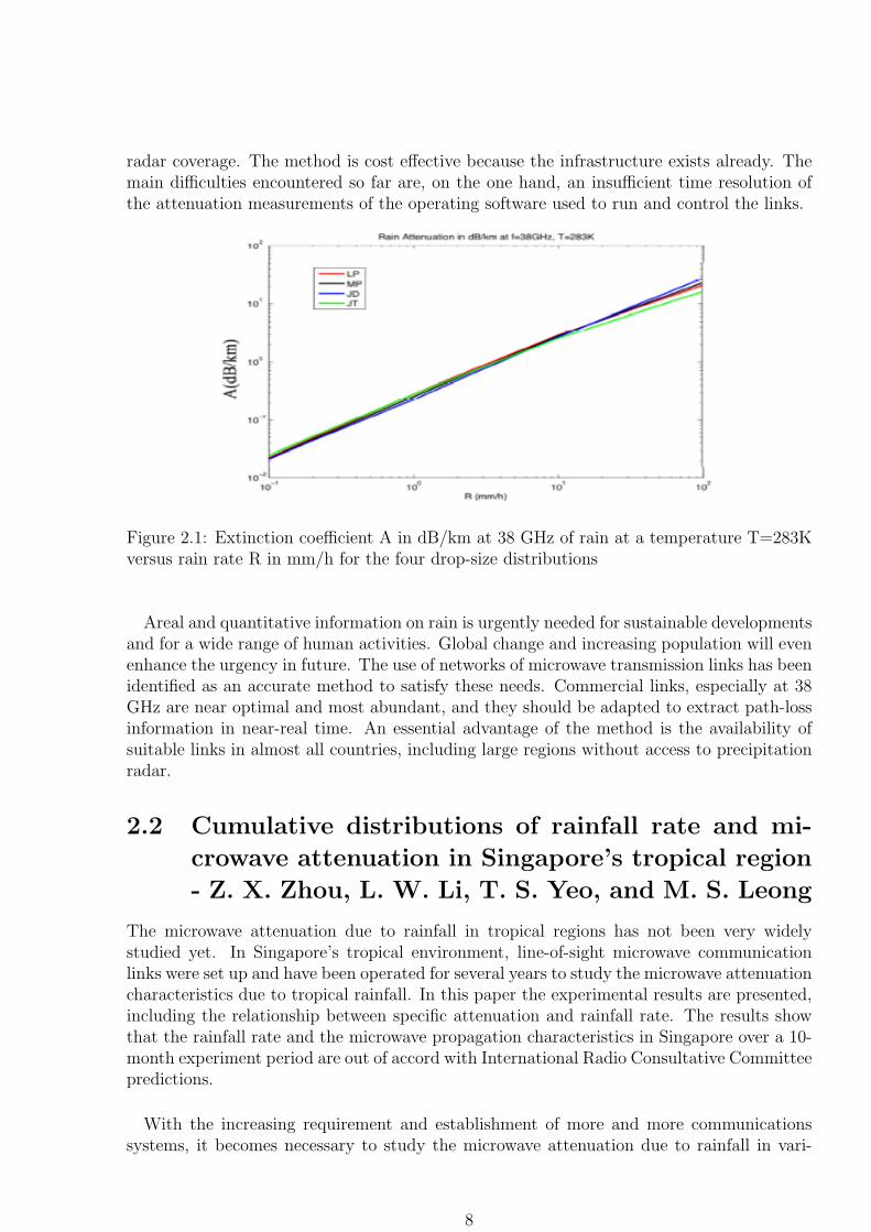
radar coverage. The method is cost effective because the infrastructure exists already. Themain difficulties encountered so far are, on the one hand, an insufficient time resolution ofthe attenuation measurements of the operating software used to run and control the links.

Figure 2.1: Extinction coefficient A in dB/km at 38 GHz of rain at a temperature T=283Kversus rain rate R in mm/h for the four drop-size distributions

Areal and quantitative information on rain is urgently needed for sustainable developmentsand for a wide range of human activities. Global change and increasing population will evenenhance the urgency in future. The use of networks of microwave transmission links has beenidentified as an accurate method to satisfy these needs. Commercial links, especially at 38GHz are near optimal and most abundant, and they should be adapted to extract path-lossinformation in near-real time. An essential advantage of the method is the availability ofsuitable links in almost all countries, including large regions without access to precipitationradar.

2.2 Cumulative distributions of rainfall rate and mi-

crowave attenuation in Singapore’s tropical region

- Z. X. Zhou, L. W. Li, T. S. Yeo, and M. S. Leong

The microwave attenuation due to rainfall in tropical regions has not been very widelystudied yet. In Singapore’s tropical environment, line-of-sight microwave communicationlinks were set up and have been operated for several years to study the microwave attenuationcharacteristics due to tropical rainfall. In this paper the experimental results are presented,including the relationship between specific attenuation and rainfall rate. The results showthat the rainfall rate and the microwave propagation characteristics in Singapore over a 10-month experiment period are out of accord with International Radio Consultative Committeepredictions.

With the increasing requirement and establishment of more and more communicationssystems, it becomes necessary to study the microwave attenuation due to rainfall in vari-

8

ous climatic zones. There exists a lot of research carried out in several countries, such asAmerica, Europe, and Japan, on the microwave propagation characteristics. The resultspublished in the literature are mainly applicable to regions of higher latitude, whereas theresults available for the tropical regions are quite limited. When the International RadioConsultative Committee (CCIR) recommended model is applied to the tropical regions, theinaccuracies of these empirical formulae are clearly seen.[2]

To study the microwave propagation characteristics, experiments have been carried outin Singapore. Previously published articles have introduced the setup of the experiment,analyzed the microwave attenuation due to rainfall at 21.225 GHz, proposed the cumulativedistributions of attenuation and attenuation duration at frequencies of 15 and 38.6 GHz,and also obtained the frequency scaling empirical formulae. As described previously, theexperimental results obtained in Singapore differ a lot from the CCIR predictions. In accordwith the CCIR recommendations, these experimental results are carefully studied again, andthe empirical formulae are proposed according to CCIR recommendations.

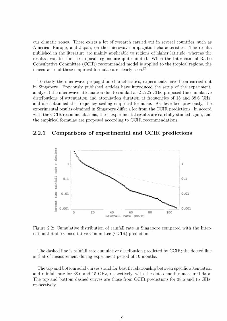
2.2.1 Comparisons of experimental and CCIR predictions

Figure 2.2: Cumulative distribution of rainfall rate in Singapore compared with the Inter-national Radio Consultative Committee (CCIR) prediction

The dashed line is rainfall rate cumulative distribution predicted by CCIR; the dotted lineis that of measurement during experiment period of 10 months.

The top and bottom solid curves stand for best fit relationship between specific attenuationand rainfall rate for 38.6 and 15 GHz, respectively, with the dots denoting measured data.The top and bottom dashed curves are those from CCIR predictions for 38.6 and 15 GHz,respectively.

9

Figure 2.3: Relationship between attenuation and rainfall rate compared with that of theCCIR at frequencies of 15 and 38.6 GHz.

It is seen that for the 10-month experiment period, the 1-min average rainfall rate dis-tribution is much different from the CCIR predictions for Singapore’s tropical environment.It is again confirmed that the CCIR recommendations have underestimated the microwavespecific attenuation due to tropical rainfall at least in the 10-month-term view. This needsto be studied further. The frequency scaling formula in Singapore in the experiment periodis also out of accord with those in literature, and it seems to follow a square root law in thefrequency range from 10 to 40 GHz. In summation, in our 10-month experiment period, therainfall rate is much smaller than predicted by CCIR for the same percent time (for example,0.01% ), while the specific attenuation is much bigger than that predicted by CCIR. It hasbeen proposed that the raindrop model and raindrop size distribution in Singapore are quitedifferent from those adopted by CCIR.

2.3 Rain Attenuation Measurements in Amritsar over

terrestrial microwave link at 19.4 & 28.75 GHz -

Ashok Kumar, I. S. Hudiara, Sarita Sharma And

Vibhu Sharma

Rain induced attenuation at 19.4 & 28.75 GHz over a terrestrial path link of 2.29 km wasmeasured for the period of one year in Amritsar (31 deg 36 degN74 deg 52 degE) environ-ment. An empirical model for predicting rain-induced attenuation on terrestrial path linkis proposed. Measured prediction has been compared with the recently prediction methodproposed by the International Telecommunication union (ITU-R). It appears that the pre-diction found differ from those predicted by ITU-R equation for the rain rate encounteredin this period.

10

System setup for the rain attenuation measurement is shown in the figure. This arrange-ment provides a dynamic range of about 45 dB at 19.4 GHz and about 47 dB at 28.75 ofexcess attenuation, which is adequate for our purpose.[3]

Figure 2.4: The measured and ITU-R rain rate

Figure 2.5: Annual cumulative percentage of time for path attenuation exceeding presentlevel

The results of one-year measurement of rain attenuation of microwave signal propagatingat 19.4 & 28.75 GHz have been presented. The annual statistics of rainfall rate and rainattenuation have been derived from the measured experimental data and compared withthose predicted by ITU-R. It is observed that ITU-R predictions underestimate the measuredrainfall rate and rain attenuation statistics.

2.4 Monitoring of rainfall by ground-based passive mi-

crowave systems:Models, measurements and appli-

cations - F. S. Marzano, D. Cimini, and R. Ware

A large set of ground-based multi-frequency microwave radiometric simulations and measure-ments during different precipitation regimes are analyzed. Simulations are performed for a

11

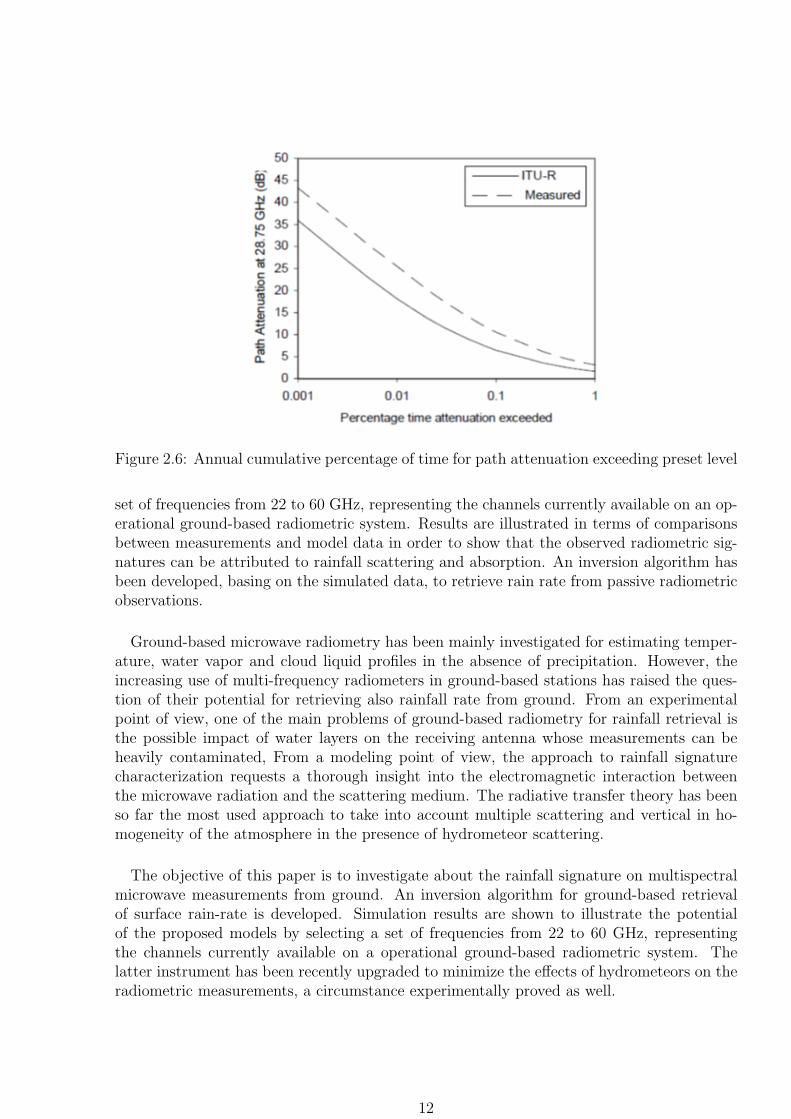
Figure 2.6: Annual cumulative percentage of time for path attenuation exceeding preset level

set of frequencies from 22 to 60 GHz, representing the channels currently available on an op-erational ground-based radiometric system. Results are illustrated in terms of comparisonsbetween measurements and model data in order to show that the observed radiometric sig-natures can be attributed to rainfall scattering and absorption. An inversion algorithm hasbeen developed, basing on the simulated data, to retrieve rain rate from passive radiometricobservations.

Ground-based microwave radiometry has been mainly investigated for estimating temper-ature, water vapor and cloud liquid profiles in the absence of precipitation. However, theincreasing use of multi-frequency radiometers in ground-based stations has raised the ques-tion of their potential for retrieving also rainfall rate from ground. From an experimentalpoint of view, one of the main problems of ground-based radiometry for rainfall retrieval isthe possible impact of water layers on the receiving antenna whose measurements can beheavily contaminated, From a modeling point of view, the approach to rainfall signaturecharacterization requests a thorough insight into the electromagnetic interaction betweenthe microwave radiation and the scattering medium. The radiative transfer theory has beenso far the most used approach to take into account multiple scattering and vertical in ho-mogeneity of the atmosphere in the presence of hydrometeor scattering.

The objective of this paper is to investigate about the rainfall signature on multispectralmicrowave measurements from ground. An inversion algorithm for ground-based retrievalof surface rain-rate is developed. Simulation results are shown to illustrate the potentialof the proposed models by selecting a set of frequencies from 22 to 60 GHz, representingthe channels currently available on a operational ground-based radiometric system. Thelatter instrument has been recently upgraded to minimize the effects of hydrometeors on theradiometric measurements, a circumstance experimentally proved as well.

12

On analysis of a large set of ground-based multi-frequency radiometric measurements andsimulations for different precipitation regimes. The modeled frequencies have been selectedin order to match the set of channels currently available on an operational ground-basedradiometric system. Rain events occurred in Boulder, Colorado and at the ARM SGP sitehave been analyzed in terms of comparisons between measurements and model data. Thiscomparison has in a way validated that the observed radiometric signatures can be attributedto rainfall scattering and absorption.[4]

2.5 Rain Attenuation Modeling In The 10-100 GHz

Frequency Using Drop Size Distributions For Dif-

ferent Climatic Zones In Tropical India - S. Das,

A. Maitra, A. K. Shukla

Rain drop size distributions (DSD) are measured with disdrometers at five different cli-matic locations in the Indian tropical region. The distribution of drop size is assumed to belognormal to model the rain attenuation in the frequency range of 10-100 GHz. The rainattenuation is estimated assuming single scattering of spherical rain drops. Different atten-uation characteristics are observed for different regions due to the dependency of DSD onclimatic conditions. A comparison shows that significant differences between ITU-R modeland DSD derived values occur at high frequency and at high rain rates for different regions.At frequencies below 30 GHz, the ITU-R model matches well with the DSD generated valuesup to 30mm/h rain rate but differ above that. The results will be helpful in understandingthe pattern of rain attenuation variation and designing the systems at EHF bands in thetropical region. Rain attenuation is a major limiting factor above 10 GHz frequency bandsto be used in radio communications. Rain attenuation modeling is usually done in terms ofdrop size distribution (DSD). But, the variability of DSD for different climatic regions is amajor concern, especially for the tropical region, which has a huge diversity in climatic con-ditions. In the absence of measured attenuation data, DSD measurements can provide usefulinformation on the variation of the rain attenuation. Rain DSD varies with rain rate as wellwith the location. Thus the same rain rate can correspond to different DSDs. Raindrop sizedistributions depend on several factors such as rainfall intensity, circulation system, type ofprecipitation, wind share, cloud type, etc. It is thus very difficult to formulate a single DSDmodel to describe the actual raindrop size distribution for all location and rain type.DSD isnormally modeled with distributions like exponential, gamma and lognormal.

The lognormal distribution is more suited for the lower end of drop spectrum due to itssteeper gradient than the gamma distribution. From the various studies over tropical region,it is found that three-parameter lognormal model is suitable for this region. Therefore, inthe present study, lognormal model is considered to be the representative distribution forDSD. Currently, Indian Space Research Organization (ISRO), as a part of earth-space prop-agation experiment over India region conducting ground based measurements at five differ-ent geographical locations, namely, Ahmedabad(AHM), Shillong(SHL), Trivandrum(TVM),Kharagpur(KGP) and Hassan(HAS). These locations fall in different climatic zones of Indiawith different rain characteristics. In the absence of actual earth-space propagation mea-surements, the attenuation modeling using DSD is attempted. This study will be helpful for

13

understanding the rain attenuation characteristics over the Indian tropical region.

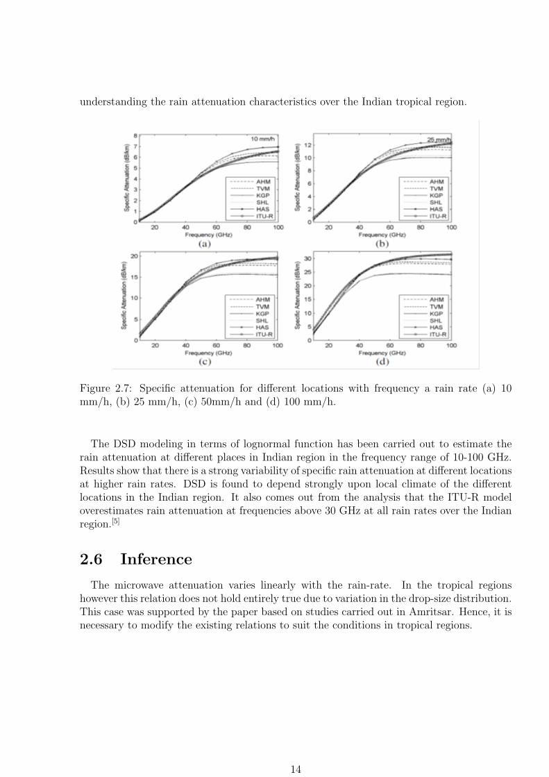
Figure 2.7: Specific attenuation for different locations with frequency a rain rate (a) 10mm/h, (b) 25 mm/h, (c) 50mm/h and (d) 100 mm/h.

The DSD modeling in terms of lognormal function has been carried out to estimate therain attenuation at different places in Indian region in the frequency range of 10-100 GHz.Results show that there is a strong variability of specific rain attenuation at different locationsat higher rain rates. DSD is found to depend strongly upon local climate of the differentlocations in the Indian region. It also comes out from the analysis that the ITU-R modeloverestimates rain attenuation at frequencies above 30 GHz at all rain rates over the Indianregion.[5]

2.6 Inference

The microwave attenuation varies linearly with the rain-rate. In the tropical regionshowever this relation does not hold entirely true due to variation in the drop-size distribution.This case was supported by the paper based on studies carried out in Amritsar. Hence, it isnecessary to modify the existing relations to suit the conditions in tropical regions.

14

Chapter 3

Basics of Rainfall Measurements

Rainfall measurement involves a number of parameters. These parameters along with rele-vant concepts and some apparatuses for rainfall measurement are illustrated in this chapter.

3.1 Rain Fall Intensity:

The intensity of rainfall is the rate at which the rain is falling and it is expressed in cm/hr.For example, during a particular event of rainfall occurred for 10 minutes and the quantityof rainfall is 2 cm, then the intensity of rainfall of that rain event is 12 cm/hr. 5 cm/ hrintensity of rainfall means an average rainfall rate of 5 cm per hour duration. The rainfallparticulars are recorded with either non-recording rain gauges or automatic recording raingauges or by Meteorological Department (IMD).

3.2 Rainfall Recording

3.2.1 Non-recording Gauges

In non-recording gauges the rainfall for the past 24 h is measured and recorded as cm ofrainfall during the last 24 hours. These data give only average intensity and not the actualintensity of rainfall of the rain event, which might have last for only 10 to 15 minutes.These types of rain gauges do not record the rain but only collect the rain. Symons’s typeinstrument is most commonly used. The rain gauge consists of a collector, with a gun metalrim, a base and a polythene bottle. The collector and the base are made of Fiber GlassReinforced (FRP). The collectors have aperture of either 100 cm2 or 200 cm2 area and areso made that they are interchangeable. The polythene bottles are of three sizes havingcapacities of 2, 4 and 10 liters of water respectively. The rain gauge should be fixed on amasonry or concrete foundation 60 x 60 x 60 cm sunk into the ground. The base of thegauge should be embedded in the foundation, so that the rim of the gauge is exactly 30 cmabove the surrounding ground level. The rim of the gauge should be kept perfectly level.The horizontality should be checked with a spirit level laid across the rim.

At the time of recording rainfall, the funnel of the rain gauge is removed and the polythenebottle taken out. The measuring jar is placed in an empty basin and the contents are pouredslowly out of the receiver into the measuring jar taking care to avoid spilling. If, however, any

15

water is spilled into the basin, its amount to the water in the measuring jar before arrivingat the total amount collected. While reading the amount of rain, the measuring jar is held,upright between the thumb and the first finger or placed it on a table or other horizontalsurface. The eye is brought to the level of the water in the measure glass and the reading ofthe bottom of the meniscus or curved surface of the water is taken. The amount of rainfallshould be read in millimeters and tenths. It is extremely important to note that the correcttype of measuring jar appropriate to the type of rain gauge funnel in use should be used formeasuring the amount of rainfall, to avoid errors in the results. A value of 0.0 is entered forno rain and a ’t’ (meaning trace) for rainfall below 0.1 mm.

The collector of the rain gauge, the receiving bottle and measuring cylinder are alwayskept clean. They should be emptied regularly of sediment or other material that may havefallen into them and cleaned periodically. The grass around the gauge should be kept short.No shrubs or plants should be allowed to grow around the gauge.

3.2.2 Automatic Recording Gauges

Automatic rain gauges record continuously the cumulative amount of water with time ona graph paper. After the collection in the bottle has recorded 10 mm of rain, the bottlegets emptied and the line representing cumulative rainfall vertically falls down. Hence, whileestimating the amount of rain fallen during any time interval, this fact must be kept in view.The graph of the automatic rain gauge shows the time taken for each 10 mm of rain. Thetotal rainfall in any particular hour can be obtained from the graph.

Recording type of rain gauges are those which can give a permanent automatic rainfallrecord without bottle reading. In this type of rain gauges, a man need not go to the gaugeto measure or read the amount of rain fallen. A mechanical arrangement by which the totalamount of rain fallen, since the record was started, gets recorded automatically in graphpaper. Thus the gauge forms a record of cumulative rain versus time in the form of a graphand which is known as the mass curve of rain fallen. The curve also helps in indicating thetimes of onset and cessation of a rain and its duration. The slope of the curve gives theintensity of rainfall for any given period.

Since such gauge represent the cumulative rain, they are called as integrating rain gauges.There are three types of recording rain gauges. They are:

• Tipping Bucket Gauge In this type of rain gauge, the rainwater is collected in thecollector and then passed through a funnel. The funnel discharges the water into a twocompartment bucket. If 0.1mm of rainwater gets filled up in one compartment, thebucket tips emptying in to a reservoir and moving the second compartment into placebeneath the funnel. The tipping bucket completes an electric circuit, causing a pen tomark on a revolving drum. These types of gauges are generally in hilly and inaccessibleareas, where they can supply measurements directly to control room. No graph paperor drum is installed in the gauge and the rainfall measurements are directly recordedat the control room.

• Weighting Type This type of gauge weights the rain which falls into a bucket placed onthe platform of a spring or a lever balance or any other weighting mechanisms .When

16

the weight of the bucket increases that helps in recording the increased quantity of rainwith time by moving a pen on a revolving drum.

• Floating Type In this type of gauge, the rise of floating body due to increasing raincatch helps in lifting the pen point, which goes on recording the cumulative rain withtime in a graph paper wrapped round a rotating drum. Nowadays various types offloating type recording rain gauges are available. Natural Siphon recording rain gaugeis widely used in India.

The rainwater entering the gauge at the top of the cover is led via the funnel to the receiver,consisting of a float chamber and a siphon chamber. A pen is mounted on the stem of thefloat, and as the water level in the receiver rises, the float arises and the pen records, on achart wrapped round a clockwise rotating drum, the amount of water in the receiver at anyinstant. The rotating drum completes one revolution in 24 hours (one day) or sometimes in7 days. Siphoning occurs automatically when the pen reaches the top of the chart, and asthe rain continues, the pen rises again from the zero line of the chart. If there is no rain, thepen traces a horizontal line from where it leaves off rising.

The siphon recording rain gauge is an instrument designed for continuous recording ofrainfall. In addition to the total amount of rainfall, the onset and cessation of rain (andtherefore the duration of rainfall) are recorded.

The gauge should be installed in such a way that the rim of the funnel is horizontal andset at a height of exactly 75 cm above ground level. For setting the pen at the zero mark,pour sufficient water into the receiver till the pen reaches the top and water siphons out.After all the water is drained out, the pen should be on the zero line; if not, it should beadjusted.

Rainfall enters the gauge at the top via a funnel and passes through a receiver consistingof a float chamber and a siphon chamber. A pen is mounted on the stem of the float, andas the water level rises in the receiver, the float rises and the pen records the level of waterin the chamber on a chart wrapped round a clockwise rotating drum. The rotating drumcompletes one revolution in 24 hours (one day) or sometimes in 7 days. Siphoning occursautomatically when the pen reaches the top of the chart, at the 10 mm mark, and then thepen comes down to the zero line of the chart. The pen rises again with the onset of rainfall.When there is no rain, the pen traces a base horizontal line of the chart.

The siphon is arranged concentrically so that the long discharge tube being surroundedby the shorter siphon chamber and is directly connected to the float chamber. A glass pieceis placed over the joint of these tubes and the passage connecting two tubes at this joint isof almost capillary dimensions, but the sectional area is large enough to discharge the watercollected in the receiver with enough speed. When the upper end of the water level fallsto a certain depth, the siphon ceases to act, the water column is broken at a definite stageby a bubble of air which gets into the capillary and freedom from dribbling is thus ensured.There is just sufficient water to float the float after siphoning.

17

The chart should be changed daily (in India at 08 30 IST) as a routine observation ir-respective of the rainfall occurrence. The observer should see that the pen trace matchesthe base horizontal line of the chart without an error after every siphoning operation. Theinstrument should be checked daily once for correct siphoning operation.

3.3 Duration of Rainfall

The duration of rainfall is the time period for which the rain event occurs at that givenintensity of rainfall. From the historic records of the automatic rain gauge station (of graphs)for 30 to 50 years the intensity of rainfalls for different time intervals such as 5 minutes, 10minutes, 15 minutes, 20 minutes, 60 minutes, etc., could be obtained.

3.4 Frequency of Rainfall

The frequency of rainfall is the number of times the rainfall of a particular intensity andduration occurred in the past based on the historic records. Frequency of rainfall is alsoknown as the recurrence interval of a particular rainfall.

3.5 The Watershed Concept

A watershed can be defined as the area of land that drains to a particular point along astream. Each stream has its own watershed. Topography is the key element affecting thisarea of land. The boundary of a watershed is defined by the highest elevations surroundingthe stream. A drop of water falling outside of the boundary will drain to another watershed.

Figure 3.1: Watershed

18

A watershed is an area of land that drains all the streams and rainfall to a common outletsuch as the outflow of a reservoir, mouth of a bay, or any point along a stream channel.The word watershed is sometimes used interchangeably with drainage basin or catchment.Ridges and hills that separate two watersheds are called the drainage divide. The watershedconsists of surface water–lakes, streams, reservoirs, and wetlands–and all the underlyingground water. Larger watersheds contain many smaller watersheds. It all depends on theoutflow point; all of the land that drains water to the outflow point is the watershed for thatoutflow location. Watersheds are important because the stream-flow and the water qualityof a river are affected by things, human-induced or not, happening in the land area ”above”the river-outflow point.

3.5.1 A watershed is a precipitation collector

Most of the precipitation that falls within the drainage area of a stream’s monitoring sitecollects in the stream and eventually flows by the monitoring site. Many factors, some listedbelow, determine how much of the streamflow will flow by the monitoring site. Imaginethat the whole basin is covered with a big (and strong) plastic sheet. Then if it rained oneinch, all of that rain would fall on the plastic, run down-slope into gulleys and small creeksand then drain into main stream. Ignoring evaporation and any other losses, and using a1-square mile example watershed, then all of the approximately 17,378,560 gallons of waterthat fell as rainfall would eventually flow by the watershed-outflow point.

3.5.2 Not all precipitation that falls in a watershed flows out

To picture a watershed as a plastic-covered area of land that collects precipitation is overlysimplistic and not at all like a real-world watershed. A career could be built on tryingto model a watershed water budget (correlating water coming into a watershed to waterleaving a watershed). There are many factors that determine how much water flows in astream (these factors are universal in nature and not particular to a single stream):

Precipitation:

The greatest factor controlling stream-flow, by far, is the amount of precipitation that fallsin the watershed as rain or snow. However, not all precipitation that falls in a watershedflows out, and a stream will often continue to flow where there is no direct runoff from recentprecipitation.

Infiltration:

When rain falls on dry ground, some of the water soaks in, or infiltrates the soil. Some waterthat infiltrates will remain in the shallow soil layer, where it will gradually move downhill,through the soil, and eventually enters the stream by seepage into the stream bank. Someof the water may infiltrate much deeper, recharging ground-water aquifers. Water maytravel long distances or remain in storage for long periods before returning to the surface.The amount of water that will soak in over time depends on several characteristics of thewatershed:

19

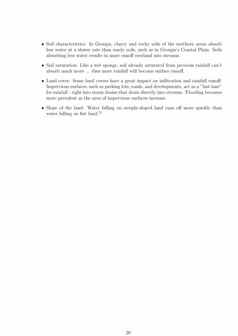
• Soil characteristics: In Georgia, clayey and rocky soils of the northern areas absorbless water at a slower rate than sandy soils, such as in Georgia’s Coastal Plain. Soilsabsorbing less water results in more runoff overland into streams.

• Soil saturation: Like a wet sponge, soil already saturated from previous rainfall can’tabsorb much more ... thus more rainfall will become surface runoff.

• Land cover: Some land covers have a great impact on infiltration and rainfall runoff.Impervious surfaces, such as parking lots, roads, and developments, act as a ”fast lane”for rainfall - right into storm drains that drain directly into streams. Flooding becomesmore prevalent as the area of impervious surfaces increase.

• Slope of the land: Water falling on steeply-sloped land runs off more quickly thanwater falling on flat land.[1]

20

Chapter 4

Rain Attenuation and Now-casting

Rain attenuation corresponds to degradation of microwave signal due to rainfall. It ispossible to use this attenuation in turn to predict rainfall rate. This rainfall has been usedto predict the time in which a particular region will get flooded, given a particular rain rate.The process of prediction whereby we get results a short time after we input parameters isknown as now-casting.

4.1 Microwave attenuation to predict rain-rate

The measurement of rainfall in urban areas is important both for design of urban drainagesystems and rainfall forecasting as input to urban drainage models (udm) to operate andcontrol drainage systems in real-time. In addition flood warning aspects have become im-portant in recent years. At present, rainfall as input to urban drainage models is deducedfrom the measurement made by rain-gauges whereas the use of radar data in urban drainagemodel is neither a new task nor a common practice

The classical rain observation uses rain gauges, which integrate rain rate over time atsingle points. Gauges measure single point rainfall and therefore their spatial significance islimited. Particularly in convective storms a series of point measurements may give a poorreflection of the areal rainfall in the catchment. Wind is known to cause systematic errors.Widespread is the use of precipitation radar giving a synoptic view of the rain dynamics overlarge areas, but due to disturbing effects, the estimation of areal rain amount appears tobe less accurate. Even though the problems connected with this measurement method, likeclutter, attenuation and Z/R relation, have to be taken care of, radar data provide valuableinformation in real time control applications.

Monitoring microwave attenuation of directional transmission links is a method to de-rive rain rate at high time resolution and in near-real time. Raindrops falling through apropagation path of a microwave link attenuate the transmitted signal quasi linearly withrain rate, allowing the estimation of path-averaged rain intensity. These data are valuablefor meteorology, hydrology, agriculture, flood control, and others. The application to en-tire networks of commercial links would be a cost-effective method to fill data gaps whereprecipitation-radar data are either distorted or missing, such as large cities, valleys in moun-tain areas and developing countries. Regionally representative rain information is neededin many areas, such as now-casting, assimilation into numerical weather prediction models,

21

hydropower, agriculture, flood control, traffic safety, pollution control, and for the validationof remote-sensing methods. The information would contribute to the reduction of socio-economic impacts of heavy rains related to flood hazards. With climate change, storms maybecome more frequent and more severe, and thus such information will become even moreimportant.

Rainfall estimation from microwave links has been a known potential for many years,but a breakthrough to operational applications is still lacking. The results of past investi-gations showed that the extinction of radiation in the frequency around 30 GHz by rain isquasi-linearly related to rain rate, and the relation is nearly independent of the drop-size dis-tribution As a consequence attenuation data at a suitable frequency are excellent to retrievepath-averaged rain rate. Such data would be representative for a real precipitation. Theuse of commercial hardware installations however poses new challenges, because commercialmicrowave networks are optimized for high communication performance and are designed inthe way that reduces the effect of weather-related impairments on quality of service. Thus,the observation type, time and magnitude resolution, network geometry and frequencies arepredefined and, in most cases, cannot be changed; records of received signal level (RSL)are distorted by quantization. Other difficulties in estimation of average rainfall per linkfrom signal attenuation include uncertainties due to variability of DSD along the link, wetantenna attenuation and uncertainty in determination of clear air attenuation due to watervapor induced attenuation and scintillation effects.

A first demonstration of the method with commercial microwave links was demonstratedin Israel. Further possibilities include attenuation data at two frequencies, at two orthog-onal polarizations, or by measuring their phase difference. The microwave attenuation dueto rainfall in tropical regions has not been very widely studied yet. The results of many ex-periments carried in Amritsar, Pakistan and Malaysia shows that prediction found in theseregion differ from those predicted by ITU-R equation for the rain rate encountered in thesame interval. The research carried out in Amritsar, proved the relation given by ITU-Rbetween attenuation and rainfall rate. In addition to that, a new relation was proposed spe-cially for that particular region which was also shown to be better than the existing ITU-Rrelation. The research in Pakistan showed that the prediction found in these region differfrom those predicted by International Telecommunication Union-Radio equation for the rainrate encountered in the same interval. Thus, the ITU-R model was not found suitable fortropical regions. The research carried out in Malaysia, on the other hand, showed that modelproposed by ITU-R was in fact better than the one shown by VIHT. An analysis of theseconditions and its results has been done as the first part of the project.[6]

4.2 Need of Now-casting

The forecasting of the weather within the next six hours is often referred to as now-casting.In this time range it is possible to forecast smaller features such as individual showers andthunderstorms with reasonable accuracy, as well as other features too small to be resolved bya computer model. A human given the latest radar, satellite and observational data will beable to make a better analysis of the small scale features present and so will be able to make amore accurate forecast for the following few hours. It is, therefore, a powerful tool in warning

22

the public of hazardous, high-impact weather including tropical cyclones, thunderstorms andtornados which cause flash floods, lightning strikes and destructive winds. In broad terms,now-casting contributes to the :

• Reduction of fatalities and injuries due to weather hazards;

• Reduction of private, public, and industrial, property damage; and to

• Improved efficiency and savings for industry, transportation and agriculture.

In addition to using now-casting for warning the public of hazardous weather, it is also usedfor aviation weather forecasts in both the terminal and en-route environment, marine safety,water and power management, off-shore oil drilling, construction industry and leisure indus-try. The strength of now-casting lies in the fact that it provides location-specific forecastsof storm initiation, growth, movement and dissipation, which allows for specific preparationfor a certain weather event by people in a specific location.

The software applications in the now-cast environment include algorithms for identifyingand tracking thunderstorm movement, identifying boundaries, wind retrieval from radar, aswell as a fuzzy-logic engine which allows the user to combine the weighted outputs fromthe various algorithms to produce a single, combined forecast. Subsequent verification ofgenerated forecasts is available both visually and statistically. In real-time operations thenow-cast environment initiates and maintains process control through an auto-restart mech-anism. The auto-restarter provides the user with an automated, hands-free forecasting en-vironment. To address issues of disaster management in India, an Indo-US collaborativeproject for improvement and modernization of the hydro- meteorological forecasting andearly warning system in India was formulated (during 2003-2008) as a part of the Govern-ment of India (GOI) US Aid for International Development (USAID) Disaster ManagementSupport Project (DMSP). Processing of Indian Doppler Weather Radar (DWR) data fornow-casting application under the sub-project Local Severe Storms and Flash Floods wasone component of this collaborative project. IMD has recently started upgrading its oldanalog radar network with a denser network of DWRs. IMD has so far installed five S-Band DWRs manufactured by Gematronik Corporation (Model: Meteor 1500S) at Chennai(2002), Kolkata (2003), Machilipatnam (2004) and Visakhapatnam (2006) replacing the oldgeneration S-Band cyclone detection radars at these stations. IMD has also installed oneindigenously built DWR at Sriharikota in 2004.

The state-of-the-art S-band Doppler Weather Radar has recently (June 2010) been in-stalled at Navy Nagar in Mumbai. The Meteorological department traditionally uses satel-lite pictures and numerical weather prediction models to forecast the rains. With the radarinstalled, it will be able to forecast the height of the cloud, direction, speed, wind activityinside the cloud. The radar will be able to locate cloud activity of around 250 km from thearea. It will also be able to accurately predict the intensity of the rainfall.

Now-casting can also be achieved by predicting rain-rate in near real-time using the mi-crowave attenuation that occurs due to rainfall. The rain-rate thus obtained can be incor-porated with a prediction system to generate forecasts.

23

4.3 Parameters that contribute to floods

Rain falling on the landscape may flow quickly over soil or rock surfaces as runoff to streamchannels. Alternately, some water may flow more slowly down-slope toward streams withinthe soil. Some may percolate downward through pores in soil and fractures in rock to reachthe top of the saturated zone (often called the water table). Below the saturated zone, it flowsmuch more slowly as ground-water.Soil characteristics, plants and animals, and slope angleare among the natural factors controlling the proportion of precipitation that is convertedto runoff in a given landscape, and the time it takes for runoff to enter a stream. Humanchanges to these landscape features can greatly influence runoff.

Grassed filter strips in farm fields help reduce runoff and erosion by slowing water veloc-ities in the vegetated areas. Grassy strips also reduce erosion by trapping excess sediment,nutrients, and farm chemicals. Vegetation (including dead vegetative materials) in prairies,forests, and other natural areas plays a similar role.

4.3.1 Infiltration:

The soil surface acts as a filter that lets water pass through (infiltrate) at a rate known asthe infiltration rate or infiltration capacity. Runoff may be produced when precipitation orsnowmelt adds water to the soil surface faster than it can be absorbed. The excess waterremains on the surface and flows down-slope as runoff. For example, if the precipitation rateis 5 centimeters (about 2 inches) per hour, but the infiltration rate is only 2.5 centimeters(about 1 inch) per hour, surface runoff is produced at the rate of 2.5 centimeters (about 1inch) per hour, even if the soil is not entirely saturated. This mechanism of runoff generationis more common in drier climates where vegetation cover is sparse.

In humid areas with greater vegetation cover, the water table may lie at the surface inlow-lying areas or slope hollows, so that the soil there is saturated. Saturated areas expandduring rain, as well as during the cold season when plants withdraw little water from thesoil. Any rain that falls on these saturated areas must run off over the surface. In times ofprolonged heavy rainfall, large areas of a gently sloping landscape may become saturated,and much of the rain that follows runs off rapidly to streams. This was the case duringthe devastating Mississippi River flood of 1993, when much of the landscape in the UpperMississippi River Basin appeared as a ”lake” on satellite images that detect surface water.

4.3.2 Soil Characteristics:

Infiltration rate is controlled by the nature of the soil, by the plant and animal communitiesit supports, and by human influences. Where soil is absent and little-fractured bedrock isexposed, water cannot soak in and will run off rapidly. If soil is present, but is very fine-grained and clay-rich, the pore spaces that water must pass through are extremely small;hence, water will infiltrate very slowly compared to sandy soils that readily soak up water.Some finer-grained soils have vertical cracks that form when the soil shrinks as it dries. Thesecracks allow water to enter more readily, but may close up after the soil is wetted.

24

Compaction of soils reduces the size of pore spaces and the infiltration rate. Water com-monly runs off areas that were compacted through repeated passage of people, large ani-mals, or heavy machinery. Raindrops falling on bare soil also can compact the soil surfacein ploughed fields, leading to increased runoff and erosion of farmland. The infiltration rateof a soil depends on factors that are constant, such as the soil texture. It also depends onfactors that vary, such as the soil moisture content.

Soil Texture

Coarse textured soils have mainly large particles in between which there are large pores.On the other hand, fine textured soils have mainly small particles in between which thereare small pores.In coarse soils, the rain or irrigation water enters and moves more easilyinto larger pores; it takes less time for the water to infiltrate into the soil. In other words,infiltration rate is higher for coarse textured soils than for fine textured soils.

The Soil Moisture Content

The water infiltrates faster (higher infiltration rate) when the soil is dry, than when it is wetAs a consequence, when irrigation water is applied to a field, the water at first infiltrateseasily, but as the soil becomes wet, the infiltration rate decreases.

The Soil Structure

Generally speaking, water infiltrates quickly (high infiltration rate) into granular soils butvery slowly (low infiltration rate) into massive and compact soils. Because the farmerscan influence the soil structure (by means of cultural practices), they can also change theinfiltration rate of his soil.

4.3.3 Plants and Animals:

In general, plants and small animals tend to increase the infiltration rate of soils. Somewater usually evaporates from plant surfaces before it can fall to the soil surface. A plantcover and litter layer of dead vegetation protects the soil surface from compaction by heavyraindrops, and also slows the delivery of water to the soil surface. Plant stems help slowdown water that flows over the soil surface. Plant roots help create openings in the soil, andalso draw water from beneath the soil surface and transpire it through leaves back to theatmosphere. Decayed plant matter helps keep fine soil particles (such as clay) from stickingtogether, thereby increasing infiltration capacity. The burrowing activities of small animalssuch as insects, worms, and gophers also help keep the soil loose and create small openingsthrough which water can pass.

When the landscape is completely de-vegetated, for example, following a forest fire orduring a construction project, a dramatic increase in runoff and soil erosion may result. Indesert environments where much of the soil surface lacks vegetation and where bare rock isexposed, most of the rainfall in heavy thunderstorms runs off rapidly and flash floods arecommon. Yet in dense, humid forests, vegetation and thick, loose soils may absorb water soreadily that water rarely runs off the surface.

25

4.3.4 Slopes

Steep slopes in the headwaters of drainage basins tend to generate more runoff than dolowland areas. Mountain areas tend to receive more precipitation overall because they forceair to be lifted and cooled. On gentle slopes, water may temporarily pond and later soakin. But on steep mountainsides, water tends to move downward more rapidly. Soils tend tobe thinner on steep slopes, limiting storage of water, and where bedrock is exposed, littleinfiltration can occur. In some cases, however, accumulations of coarse sediment at the baseof steep slopes soak up runoff from the cliffs above, turning it into subsurface flow.

4.3.5 Runoff and Flooding

Water commonly flows down-slope through the loose soil overlying bedrock. This watermoves more slowly to streams than does surface runoff. Rain falling on areas where un-fractured bedrock is exposed has little opportunity to infiltrate, and instead will run off thesurface. A brief thunderstorm in Yellowstone National Park produced considerable surfacerunoff from these steep cliffs much less likely to cause flooding, but is faster than the creepingflow of groundwater in the bedrock below.

4.3.6 Runoff and Urban Development

Urban development can greatly increase the amount of precipitation that is converted torunoff in a drainage basin. Most paved surfaces and rooftops allow no water to infiltrate,but instead divert water directly to storm channels and drains. Urbanization is of seriousconcern to water resources for several reasons.

First, the increased amount of water flowing to streams during storms causes larger floods,and floods build to a peak faster because of the rapid flow of water over smooth surfaces.

Second, motor vehicles leave oils and exhaust residues on streets, and household andindustrial chemicals also collect on pavement surfaces. These nonpoint-source pollutantsare readily washed off during storms, contaminating streams into which urban runoff flows.Careless disposal of hazardous wastes on streets or in storm drains adds to the problem.

Third, most precipitation has no chance to percolate downward to groundwater, so thesupply of groundwater to wells is reduced.

Some cities have taken steps to reduce these impacts. Pavement can be constructed sothat some water passes through to recharge groundwater, and storm runoff can be routed toartificial basins that allow water to soak in. Along with regulation of hazardous industrialwastes, programs have been developed to educate the public about the dangers of improperdisposal of wastes on streets and in storm drains.

Flooding can happen anywhere, whether near to watercourses or not. Floods can evenoccur during summer months when thunderstorms trigger torrential downpours.

26

4.3.7 Drainage system

The drainage system sometimes cannot cope with the magnitude of water that collects onsurrounding surfaces, especially when they are already saturated with large quantities ofwater. In this case, even a small amount of additional rainfall can cause flooding.

Flooding can be caused by cracks in broken pipes owned by water companies and heavierthan normal rainfall that causes water to run onto roads from fields and over-full rivers. Itcan also be caused by the collection of mud, leaves and other debris that block drains.

4.3.8 Tides

The chance of big waves meeting ocean-bound runoff has communities taking protectivemeasures. Heavy rains combined with a high tide over six feet can lead to severe coastalfloods. The high tides prevent the rain-water from draining into the oceans resulting inheavy floods in the coastal areas. There have been many instances of flooding due to rainswhen they are accompanied by high tides. These conditions are always a concern in allcoastal cities including Mumbai.

27

Chapter 5

Flood Prediction System

The probability of floods in a particular region depends not only on the amount andduration of rainfall but also on a number of other influential factors. An effective floodprediction system thus should take into account all the above factors for accurate forecast.

Our undertaking though not elaborate has aimed to work on similar lines. It takes intoaccount the rain-rate along with the topography of an area to predict possibility of floods.The basic idea is based on the fact is that in case of rainfall the low-lying regions are morelikely to get flooded, the water then eventually moving to the other areas. This can givea fair idea of the time in which the any region under consideration is likely to flood. Thisconcept has been implemented by dividing the area into watersheds. A watershed is a basin-like landform defined by highpoints and ridgelines that descend into lower elevations andstream valleys.

5.1 Defining the topography:

The topography of an area is defined in terms of latitude, longitude and height above thesea level of various points in the area under consideration. The number of points recordeddepends on the desired accuracy of representation of topography. The greater the numberof points more accurate is the reconstruction of an area.

For the sake of demonstration and verification the region from Vile Parle (West) to Jogesh-wari (West) in Mumbai. A total of 1500 locations were recorded taking into considerationthe three defining parameters. Depending on the availability and accuracy of data around1004 points were considered for the final observation. The data required was collected fromthat available on Google maps. The amount of data required is not precisely available withthe BMC and can be most accurately recorded from the services provided by Google maps.

5.2 Creating a grid of recorded data:

A point with lowest value of latitude and longitude is taken as the origin also termed asthe reference point. The relative positions of all other recorded points with respect to thereference are calculated. This relative positioning is of utmost importance in recreating thetopography with exact locations and dimensions for the new grid.

28

The dimensions of the grid are then fixed depending on the desired resolution and theneed of representation. The area is then divided into intervals along length and width toform a suitable grid. All the points lying with a given cell of the grid are noted. The averageheights of all the points is calculated and assigned to the cell. This cell represents the areaenclosed by the intervals along length and the breadth. The initial total number of points isthus grouped according to their location and their average heights determined. This processis termed as Grid Averaging.

5.3 Finding the number of sinks:

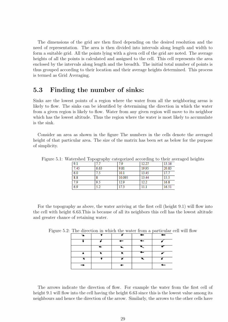
Sinks are the lowest points of a region where the water from all the neighboring areas islikely to flow. The sinks can be identified by determining the direction in which the waterfrom a given region is likely to flow. Water from any given region will move to its neighborwhich has the lowest altitude. Thus the region where the water is most likely to accumulateis the sink.

Consider an area as shown in the figure The numbers in the cells denote the averagedheight of that particular area. The size of the matrix has been set as below for the purposeof simplicity.

Figure 5.1: Watershed Topography categorized according to their averaged heights

For the topography as above, the water arriving at the first cell (height 9.1) will flow intothe cell with height 6.63.This is because of all its neighbors this cell has the lowest altitudeand greater chance of retaining water.

Figure 5.2: The direction in which the water from a particular cell will flow

The arrows indicate the direction of flow. For example the water from the first cell ofheight 9.1 will flow into the cell having the height 6.63 since this is the lowest value among itsneighbours and hence the direction of the arrow. Similarly, the arrows to the other cells have

29

been assigned. The blank cells indicate that the corresponding regions only receive waterfrom their neighboring areas and itself cannot contribute to water accumulation in any otherregion. These areas are the sink regions. These directions also play a role in determining thewatersheds in an area. A sink and the regions contributing to water accumulation in thatsink together form a watershed.

5.4 Finding the watershed

Initially every regions is denoted by ’1’.For every cell that contributes to accumulation in aparticular regions the count for that particular region is incremented by ’1’.Thus the totalnumber of regions contributing to accumulation in a given area (cell) can be calculated.Accordingly the above representation is transformed into the following figure.

Figure 5.3: Watershed table

Sinks however are not just the lowest regions; they are those regions which only receivewater and do not contribute to flooding in other areas. Thus for the given topography thesinks occur at points with altitude 6, 5.2 and 11.1.All heights being taken in meters. Thedirection of flow thus plays a crucial role in identifying a watershed, since a region maybe atthe lowest elevation but it may not be a sink.

Once a particular region is filled with water it will overflow to the neighbor having thelowest height. Extending this concept to the watersheds, water will flow from one watershedto the next over the smallest height. This height is known as the spill height. The watershedsare thus assumed to be connected to each other by their spill-heights. As shown in the figurebelow.

Figure 5.4: Watershed connected by their spill heights

30

The circles denote the watersheds with their sink values specified. The links give thevalues the lowest height common to the watershed over which the water will move to thenext watershed. The bidirectional nature of the links indicates that water may flow fromeither region to the other depending on the extent of accumulation in those regions.

5.5 Flooding

The process of flooding of each area can be defined by taking into consideration the volumeof a cell and its fill rate.

Volume of any cell is given by Area of a cell X Height up to which the water willfill before flowing over.

Fill Rate is defined as the time taken for a particular area to fill. It is given as

Rain-rate *No of cells

Therefore,

Spill Time = Volume/Fill Rate

When an area under consideration experiences rainfall the rain water as well as the waterfrom the neighboring areas flows into the sinks. The sinks once underwater the additionalwater overflows into the neighboring areas.

Once a watershed is completely inundated water from that region will move into theneighboring watershed over the smallest height. Thus the two watersheds merge effectivelythough not physically. Thus the effective volume and spill time changes for the new apparenttopography. Therefore every time watersheds merge the topography changes apparently andhence the spill time and spill volume until finally the region is submerged.

Thus if the rain-rate is known the amount of time in which a region will be flooded can bedetermined. Also similarly the extent to which a given area will be flooded in a particulartime for a particular rain-rate can be determined. Thus floods can be predicted.

Along with the basic topography, a number of parameters contribute to flooding. Anintegration of these parameters is important for well defined accurate predictions. Howeverdue to insufficient data the other parameters have not been included.[2][3]

31

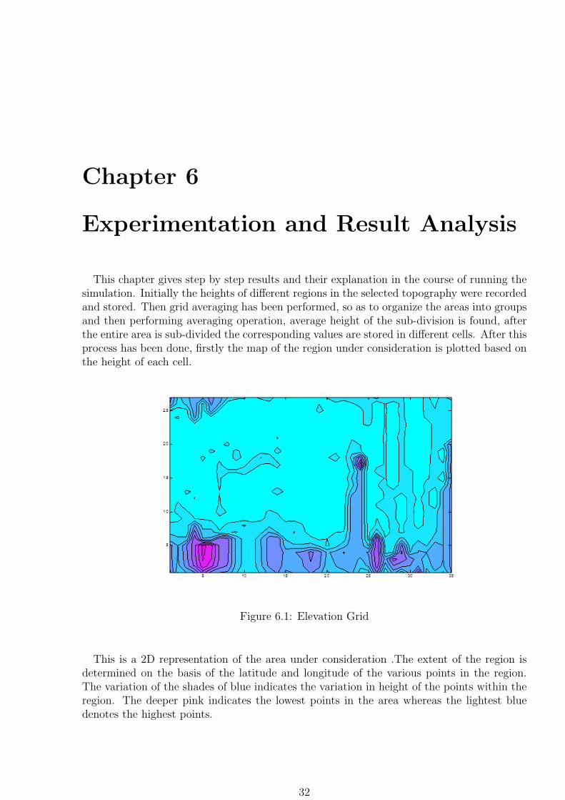
Chapter 6

Experimentation and Result Analysis

This chapter gives step by step results and their explanation in the course of running thesimulation. Initially the heights of different regions in the selected topography were recordedand stored. Then grid averaging has been performed, so as to organize the areas into groupsand then performing averaging operation, average height of the sub-division is found, afterthe entire area is sub-divided the corresponding values are stored in different cells. After thisprocess has been done, firstly the map of the region under consideration is plotted based onthe height of each cell.

Figure 6.1: Elevation Grid

This is a 2D representation of the area under consideration .The extent of the region isdetermined on the basis of the latitude and longitude of the various points in the region.The variation of the shades of blue indicates the variation in height of the points within theregion. The deeper pink indicates the lowest points in the area whereas the lightest bluedenotes the highest points.

32

Further, based on the heights of cells, the sinks present in the region under considerationare found out. Sink is said to be the cell where water gets accumulated. The cells contributingto a particular sink together form a watershed.

The model displays the topography of the region under consideration. In addition it alsogives the time required for a particular region to get flooded. The flowing are the simulationresults of the model.

Figure 6.2: Watershed Map

This is known as a watershed map. Each different color denotes a different watershed (asink and all areas contributing to that sink) .The watersheds border on a number of differentwatersheds to form the complete area under consideration. A single color represents themean height of that particular watershed above the sea-level.

Each node represents a sink within a watershed. The number of nodes therefore is equalto the number of sinks i.e number of watersheds. The watersheds (nodes) are shown to beconnected to the bordering watersheds with links .The lowest height on the boundary isspecified on the link i.e it denotes the path through which water from a particular watershedwill spill out on overflowing. All links are bi-directional to indicate that the water mayoverflow from any region that fills in earlier in time to its neighbor.

This is the 3D representation of the area under consideration. The X-Y plane defines thegeographical extent of the area .The Z axis gives the height of the individual regions abovethe sea-level. The shown region is mapped based on the latitude and longitude of the pointswithin the region and their relative positions from each other.

The following is the a succession of images of the simulation displaying the flooding of aparticular region.The region considered here is the watershed number 40 .The unit rainfalland the time of rain are also specified. This is the 3D representation of the area underconsideration. The X-Y plane defines the geographical extent of the area .The Z axis givesthe height of the individual regions above the sea-level. The shown region is mapped based

33

Figure 6.3: Watershed Graph

on the latitude and longitude of the points within the region and their relative positionsfrom each other.

34

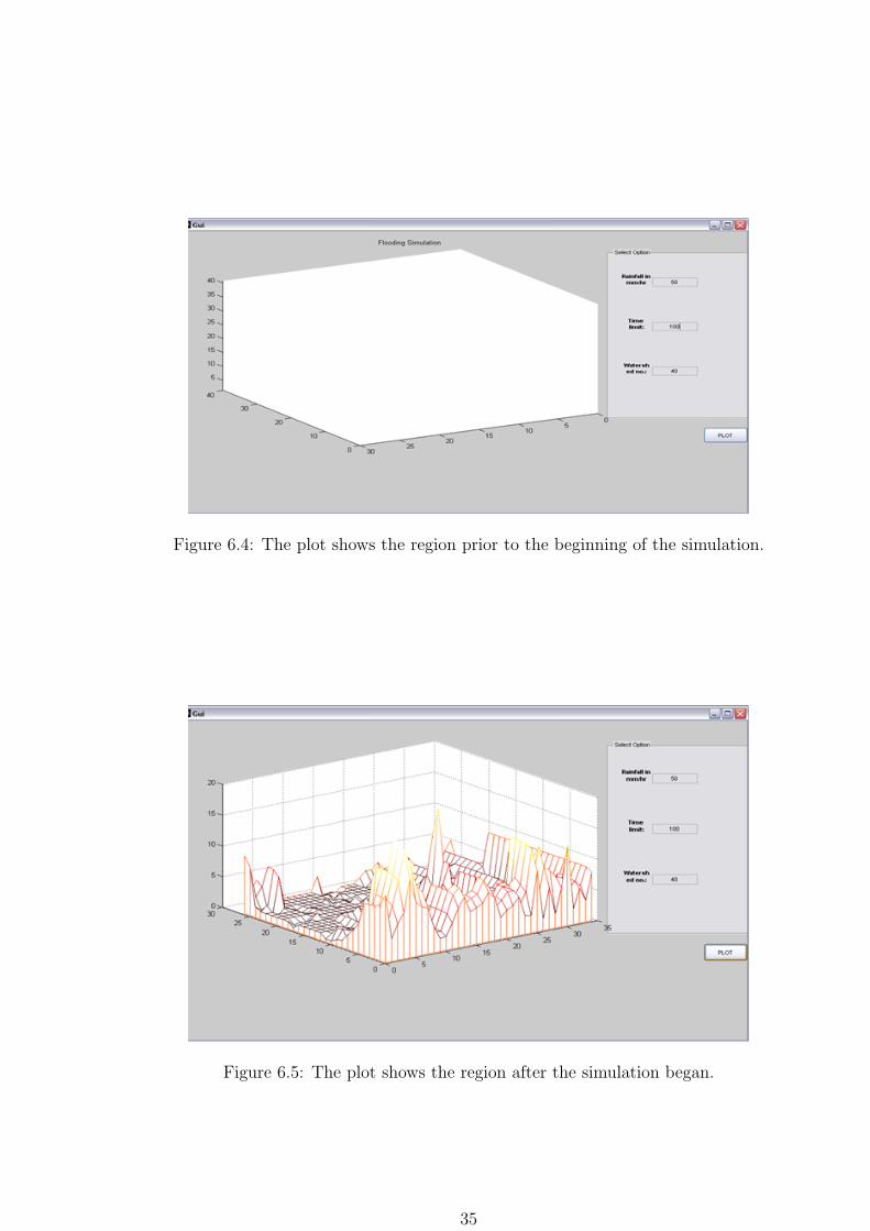
Figure 6.4: The plot shows the region prior to the beginning of the simulation.

Figure 6.5: The plot shows the region after the simulation began.

35

Figure 6.6: The plot shows the area getting flooded (marked in red)

Figure 6.7: The plot shows different regions getting flooded (marked in red)

36

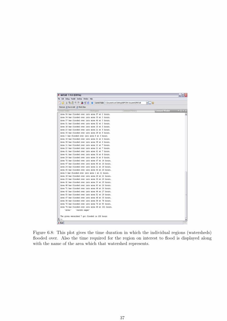
Figure 6.8: This plot gives the time duration in which the individual regions (watersheds)flooded over. Also the time required for the region on interest to flood is displayed alongwith the name of the area which that watershed represents.

37

Chapter 7

Comparison of Rain AttenuationModels

This section gives the comparison between various rain attenuation models with the ITU-Rmodel,which give a relationship between rain rate and microwave attenuation due to rain.

The models generally fall into two categories: (a) those that attempt to define the physicsof the process and (b) those that use empirical approaches with simplified assumptions. Dueto the lack of world-wide information on many of the physical inputs needed to provideaccurate results using the models of type (a), type (b) models - empirical procedures - havetended to be used most often and with usually the best results.

It has been reported that most of the available rain attenuation prediction models providean annual average accuracy of the order of 30%.The model accuracy reported is supportedby recent testing efforts in the ITU-R. A lower limit to the prediction accuracy for rainattenuation models is set by the natural variability of the rain process itself, which is thoughtto be around 20% on an annual basis. Results indicate that the rain attenuation element ofthe model provides the best average accuracy globally between 10 and 30 GHz and that thecombined procedure gives prediction accuracies comparable to uncertainties associated withthe year-to-year variability of path attenuation.

7.1 ITU-R Model

The Crane and other models were believed to overestimate the attenuation compared tothe CCIR model. Yamada used 124 data sites and proposed changes to the CCIR modelthat are represented in the present ITU model. After improvement to the CCIR method,errors in the mean attenuation were less than 20% at availabilities of 99.9% or better.

For prediction of rain fade attenuation using the ITU 530 standard, rain rate at the 0.01%exceeded level for the zone of interest is required, frequency, path length, frequency, andattenuation factors from ITU-R 838 . The ITU model consists of simple equations and isknown for ease of use.[9]

38

Figure 7.1: The ITU-R model

7.2 The Indian Model

The proposed rain attenuation prediction model is somewhat similar to the one recom-mended by the ITU-R where the rain related input to the model is the rain intensity at the0.01% probability level. The method was derived on the basis of the log-normal distribu-tion using similarity principles. Both point rain intensity and path attenuation distributionsgenerally conform to the log-normal distribution. In homogeneity in rain in the horizontaland vertical directions are accounted for in the prediction. The same procedure applies forboth slant paths and terrestrial paths. The method is applicable across the frequency range4 to 35 GHz and percentage probability range 0.001% to 10%.

Rain zone models such as the ITU-R and Crane global model embody broader climaticfeatures of widely separated regions. As such, they tend to be rather coarse and may not

39

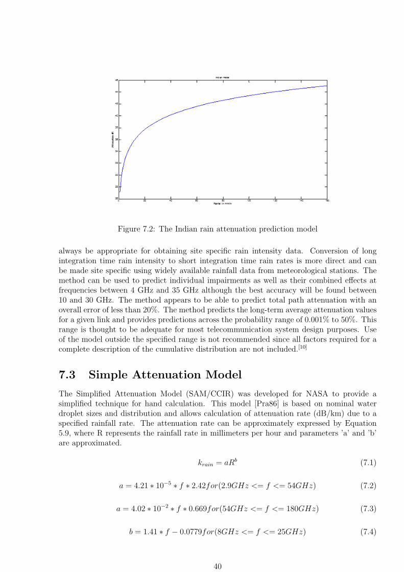
Figure 7.2: The Indian rain attenuation prediction model

always be appropriate for obtaining site specific rain intensity data. Conversion of longintegration time rain intensity to short integration time rain rates is more direct and canbe made site specific using widely available rainfall data from meteorological stations. Themethod can be used to predict individual impairments as well as their combined effects atfrequencies between 4 GHz and 35 GHz although the best accuracy will be found between10 and 30 GHz. The method appears to be able to predict total path attenuation with anoverall error of less than 20%. The method predicts the long-term average attenuation valuesfor a given link and provides predictions across the probability range of 0.001% to 50%. Thisrange is thought to be adequate for most telecommunication system design purposes. Useof the model outside the specified range is not recommended since all factors required for acomplete description of the cumulative distribution are not included.[10]

7.3 Simple Attenuation Model

The Simplified Attenuation Model (SAM/CCIR) was developed for NASA to provide asimplified technique for hand calculation. This model [Pra86] is based on nominal waterdroplet sizes and distribution and allows calculation of attenuation rate (dB/km) due to aspecified rainfall rate. The attenuation rate can be approximately expressed by Equation5.9, where R represents the rainfall rate in millimeters per hour and parameters ’a’ and ’b’are approximated.

krain = aRb (7.1)

a = 4.21 ∗ 10−5 ∗ f ∗ 2.42for(2.9GHz <= f <= 54GHz) (7.2)

a = 4.02 ∗ 10−2 ∗ f ∗ 0.669for(54GHz <= f <= 180GHz) (7.3)

b = 1.41 ∗ f − 0.0779for(8GHz <= f <= 25GHz) (7.4)

40

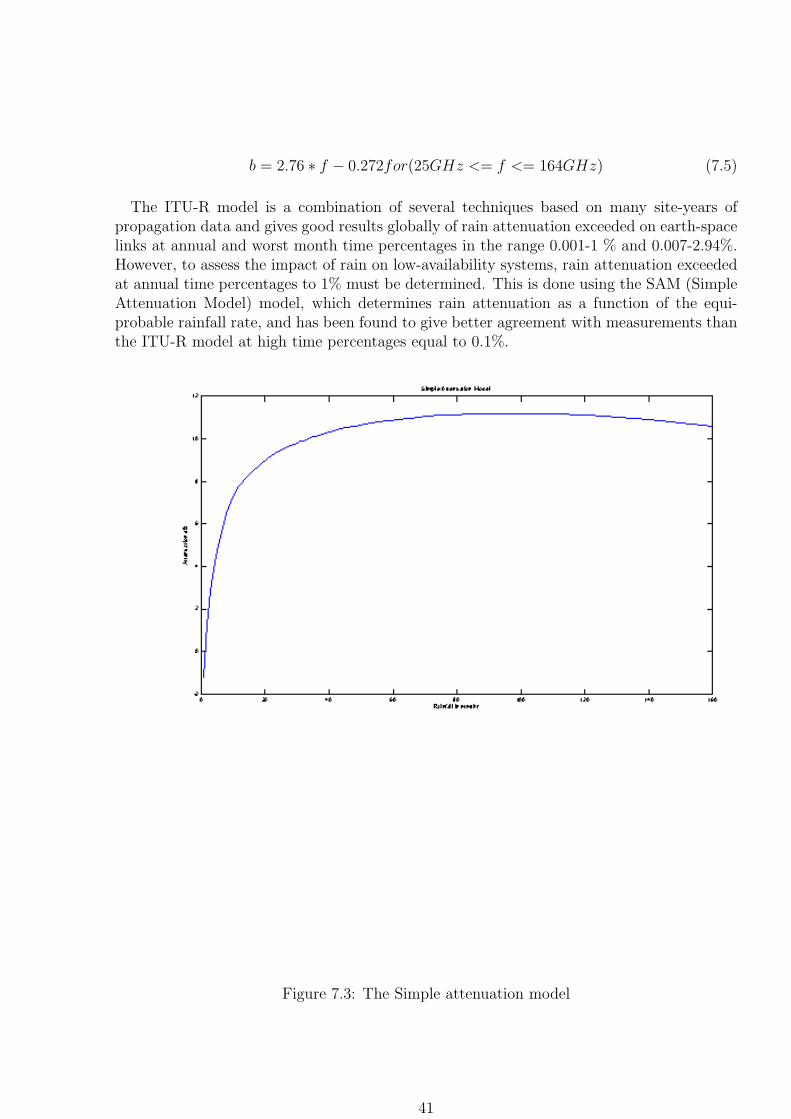
b = 2.76 ∗ f − 0.272for(25GHz <= f <= 164GHz) (7.5)

The ITU-R model is a combination of several techniques based on many site-years ofpropagation data and gives good results globally of rain attenuation exceeded on earth-spacelinks at annual and worst month time percentages in the range 0.001-1 % and 0.007-2.94%.However, to assess the impact of rain on low-availability systems, rain attenuation exceededat annual time percentages to 1% must be determined. This is done using the SAM (SimpleAttenuation Model) model, which determines rain attenuation as a function of the equi-probable rainfall rate, and has been found to give better agreement with measurements thanthe ITU-R model at high time percentages equal to 0.1%.

Figure 7.3: The Simple attenuation model

41

The attenuation increases with an in increase in rainfall. However the characteristics alsoexhibit a fall in attenuation at higher values of rainfall which does not satisfy the generalrule and hence questions the credibility of the model.[11]

7.4 Crane Model

The ”Crane” models, after Robert K. Crane, are popular for satellite-earth links but alsohave terrestrial models.

In the equations below ,AR is the rain attenuation in dB, R is the point rain-rate inmm/hr, and d is the distance in km. Constants ’a’ and ’b’ are rain attenuation coefficientsthat are functions of frequency and polarization and are tabulated.

A = aRb ∗ (eubd − 1)/ubfor0 <= d <= D0 (7.6)

A = aRb ∗ ((eubD0 − 1)/ub− (BbecbD0)/cb+ (Bbecbd)/cb) (7.7)

D03.8− 0.6ln(R) (7.8)

B = 2.3R( − 0.17) (7.9)

u = ln(B ∗ e(c ∗D0))/D0 (7.10)

c = 0.026 + 0.03ln(R) (7.11)

For paths longer than 22.5 km, the attenuation AR is calculated for a 22.5 km path, andthe resulting rain attenuation is multiplied by a factor of (d /22.5). The Crane rainfall zonesare defined differently than the ITU zones with more defined zones in the US than the ITUzones. The Crane models predict a larger attenuation than the ITU model. Calculation bythe ITU model is straightforward by scaling the 0.01% rain rate and by using an effective pathlength reduction factor to account for the cellular nature of heavy rainfall. Mean cumulativedistributions of rainfall zones are defined geographically in ITU-R 837.

The Crane Global model requires solution of about 8 equations to obtain the path-averagedrain rate and a piecewise representation of the path profile by exponential functions. Theinitial two-component Crane model first computes the volume cell contribution from thepath integrated rain rate produced by a volume cell and the debris contribution based onthe length scale for the debris path. About 10 equations are involved.

For the revised two-component Crane model, spatial correlation functions are includedand an integral equation for the debris path. It also includes a prediction for satellite pathdiversity.

42

Figure 7.4: The Crane model

7.5 Earth to Space Model

Rain attenuation modeling on satellite paths has been done by many researchers over thelast three decades. With the introduction of Ku-band satellite communication services inthe tropical and equatorial region, prediction of rain attenuation has become an importantfactor. Several empirical and non-empirical rain attenuation prediction models that havebeen developed are based on the measurement data obtained from temperate regions. Mostof these existing rain attenuation prediction models do not appear to perform well in highrainfall regions.

The ITU-R model is currently being widely used by many researchers. Cumulative distri-bution empirical evidence shows that the ITU-R model underestimates the measured rainattenuation cumulative distribution when applied to tropical regions, leading to a poor pre-

43

diction. Therefore a modified ITU-R model was developed using the complete rainfall ratecumulative distribution and the horizontal path length to calculate the cumulative distribu-tion of rain attenuation for tropical and equatorial regions.

The modified ITU-R model retains the concept of an equivalent rain cell. The horizontalprojection of the slant path, LG was modified based on the rain height, elevation angle,reduction factor, and the rainfall rate at the measurement sites. Therefore this model wasrevised, so that it can be used at tropical countries with the antenna elevation angle varyingfrom 400 to700. In the ITU-R model, the rainfall rate exceeded at 0.01% of time is used forpredicting the correspondent value of rain attenuation. The extrapolation formula was alsoused to calculate the rain attenuation exceeded at other percentages of time between 1%and 0.001%. In the proposed model, the extrapolation formula was modified based on therain attenuation data obtained from the measurement sites. The rain attenuation exceededduring P% of time is then given by:

Ap = A0.01 ∗ 0.12 ∗ p−(0.58569 + 0.06104log(P ))dB (7.12)

Where, A0.01is the rain attenuation exceeded at 0.01% of time. The specific attenuationis a function of the rainfall rate, R0.01 exceeded at 0.01% of time is given by:

γ = k(R0.01)αdB/km (7.13)

Where, k and α are frequency and polarization parameters. The horizontal reductionfactor, r0.01 exceeded at 0.01% of time is given by:

r0.01 = (1 + LG/Lo)−1 (7.14)

where, Lo is equivalent rain cell length and LG is horizontal projection of the slant pathcalculate by using the rain attenuation data at the measurement site. This parameter isgiven by:

LG = (3167.9714+2088.3369(LS cos(θ))−66.345562(LS cos(θ))2−2182.7255(ln(LS cos(θ)))2+1229.5222(LS cos(θ))2)(7.15)

Where, LSis the slant path length and θ is the antenna elevation angle.The rainfall attenuation, A0.01 exceeded at 0.01% of time is given by:

A0.01 = γ ∗ r0.01 ∗ LS (7.16)

The mean error, µe and standard deviation, σe are used to calculate the Root Mean Square,De(RMS).

The parameter is defined as follows:

De = (µ2e + σ2

e)0.5 (7.17)

According to evaluation procedures adopted by the CCIR the preferred prediction methodis the one producing the smallest RMS values.

44

On comparison it is seen that the proposed rain attenuation model for earth-to-spaceperformed better than the ITU-R model. The model can be used for different elevationangles and it is simply to use.

Figure 7.5: The Earth to Space Improved Model

According to evaluation procedures adopted by the CCIR the preferred prediction methodis the one producing the smallest RMS values.

On comparison it is seen that the proposed rain attenuation model for earth-to-spaceperformed better than the ITU-R model. The model can be used for different elevationangles and it is simply to use.

45

7.6 Tropical Model

Rain attenuation is a major limiting factor above 10 GHz frequency bands to be used inradio communications. It is also a relevant issue for space-borne radars for cloud and precip-itation characterization. Although, other forms of hydrometeors (snow, hail etc) also affectthe performance of the system, the attenuation due to rain is most severe. Rain attenuationmodeling is usually done in terms of drop size distribution (DSD). But, the variability ofDSD for different climatic regions is a major concern, especially for the tropical region, whichhas a huge diversity in climatic conditions. A few attempts have been made to characterizethe rain attenuation over this region. In the absence of measured attenuation data, DSDmeasurements can provide useful information on the variation of the rain attenuation.

Rain drop size distributions (DSD) were measured with disdrometers at five differentclimatic locations in the Indian tropical region. The distribution of drop size is assumed tobe lognormal to model the rain attenuation in the frequency range of 10-100 GHz. The rainattenuation is estimated assuming single scattering of spherical rain drops. A comparisonshows that significant differences between ITU-R model and DSD derived values occur athigh frequency and at high rain rates for different regions. At frequencies below 30 GHz,the ITU-R model matches well with the DSD generated values up to 30mm/h rain rate butdiffer above that.

To estimate the direct relationship between rain fall rate and the rain attenuation, nor-mally, a power-law relationship of the following form is considered according to ITU-R stan-dard.

A = k(Rα) (7.18)

Where k and α are constants.

From the regression analysis of the modeled attenuation with the rain rate, the constantsare again determined for different locations and different frequencies in the tropical regionas shown. In the table below SHL stands for Shillong, AHM stands for Ahmedabad, TVMstands for Tiruvananthapuram, KGP stands for Kharagpur and HAS stands for Hasan.

The DSD modeling in terms of lognormal function has been carried out to estimate therain attenuation at different places in Indian region in the frequency range of 10-100 GHz.Results show that there is a strong variability of specific rain attenuation at different lo-cations at higher rain rates. DSD is found to depend strongly upon local climate of thedifferent locations in the Indian region. It also comes out from the analysis that the ITU-R model overestimates rain attenuation at frequencies above 30 GHz at all rain rates overthe Indian region. At smaller rain rates and in the frequency range 10-30 GHz, the ITU-Rmodel performs well. It is found that for higher rain rates, specific attenuation values varysignificantly at different locations and also differ from the ITU-R model. The results will behelpful in understanding rain attenuation variation and designing communication systemsat EHF bands in the Indian regions.

46

Figure 7.6: k and a for different regions are given at different frequencies

Firstly, the proposed system requires the measurement of rainfall of a given region. Thetraditional method to measure rainfall has been with the help of rain gauges. The gauges areof two types viz., non-recording and automatic recording gauges. The non-recording gaugesare used less and automatic recording ones are preferred. The automatic recording gaugesrecord the cumulative amount of water with time continuously on graph paper. Thus theaccuracy of automatic rain gauges is more as it gives more number of readings. In addition tothis method satellite imagery is also used but it is not sufficiently efficient for fast prediction.

It is also possible to extract rainfall data from the amount of corresponding microwaveattenuation. In other words, the amount of rainfall of a given region can be found out byusing the information regarding the extent of degradation of microwave signals. There are anumber of relations that are used to give more accurate results than the other. The factor tobe taken into account, is, which one of these models gives most accurate results for the region

47

under consideration. Thus it can be seen that the ITU-R relation has definite flaws when itcomes to implementation in tropical regions. This can be traced to high amounts of rainfallin tropical regions and corresponding drop sizes. Further, depending upon the region underobservation, appropriate relation can be chosen so as to measure the rainfall rate throughthe use of microwave attenuation data. The advantage of using microwave attenuation datafor calculation of rain-rate is the prospect of monitoring the system on a real-time basis.This brings to light the concept of now-casting which enables the authorities to keep an eyeon natural disasters like rain-flood and take necessary action before the situation worsens.

Secondly, the proposed system involves the calculation of time in which a particular regionmight get flooded when provided with the intensity of rainfall in mm/hr. This time that ispredicted is known as spill time. Most of the current systems have low sensitivity, that is,they are slower to respond to extreme flood causing events like rain flood. The reasons behindit are the lack of continuous monitoring of rainfall rate and an absence of any fixed algorithmfor prediction of flooding time. There exists an algorithm which has been usually used topredict river floods in a particular area. The proposed system, thus, involves integration ofthis algorithm to predict rain-floods, that is, to predict the time required for a given areato get flooded. This algorithm takes rainfall rate at a given instant of time along with theheights of sectors within the area under consideration as input and gives the spill time of thatarea. The data regarding heights of different regions within the area needs to be recorded.The rainfall data required can be obtained from the earlier method, that is, from microwaveattenuation. The advantage of this system is that since the rainfall rate can be continuouslymonitored through measurement of microwave attenuation, corresponding spill time can becalculated at the same rate. The topographic data that is the data regarding heights ofregions within the areas can be stored beforehand. As the rain rate gets fed as input to thesystem in real time, the spill time of any desired region within the area under considerationcan be calculated equally efficiently. Thus, in case of extreme events the response time ofthe system would be much less. As a result, the process of issuing of warnings can be spedup so as to prevent the loss of human life as well as proper.

48

Chapter 8

Conclusion and Future Work

8.1 Conclusion

The relation proposed by the ITU-R does not provide accurate results for the tropicalregions. It can be modified to according to the conditions in the tropical region. The mainreason for the variation in attenuation due to rainfall in the tropical regions is the higheramount of rainfall and different drop size distribution. Although efforts have been madeto develop a relation suitable for the tropical regions no particular relation has yet beendeveloped.

The method of flood prediction proposed in this project gives satisfactory results for thearea considered. The time required for the particular area to get flooded for a particular rateof rain can be determined successfully. However due to limited number of input parametersconsidered the large scale application of the project is restricted.

8.2 Future Work

The need of the hour is a system that provided faster flood prediction in cities. It canonly be achieved a means of faster rain-rate measurements accompanied by the knowledge oftopographical and structural characteristics of a region to achieve more accurate prediction.

Therefore, efforts to determine an improved relation between the rain-rate and correspond-ing attenuation in the tropical region are crucial for accurate rain-rate measurements. Inaddition elaborate details about the structure and topography of an area are important .Thiswould require the assimilation of all factors contributing to floods. A model incorporatingthe drainage system, soil and the plan of a city in addition to basic topography is requiredfor accurate results.

Thus a complete system comprising of all the necessary parameters should be the goalfor the future. Also the prediction results can be relayed to the concerned individuals withmeans of broadcast system taking input from the prediction model. The system could bea simple GSM modem. A wise combination of all the above can thus provide a absolutesystem for flood prediction in flood prone cities like Mumbai.

49

Bibliography

8.3 Reference Papers

[1] Christian Mtzler, Ernest Koffi and Alexis Berne (2009) -’Monitoring Rain Rate withData from Networks of Microwave Transmission Links’, EUCAP, Berlin.

[2] Z. X. Zhou, L. W. Li, T. S. Yeo, and M. S. Leong(June 2000)-’Cumulative distributionsof rainfall rate and microwave attenuation in Singapore’s tropical region’, Radio Science,Vol.35 ,No 3.

[3] Ashok Kumar, I. S. Hudiara, Sarita Sharma and Vibhu Sharma (2009) - ’Rain Attenu-ation Measurements in Amritsar over terrestrial microwave link at 19.4 & 28.75 GHz’,Guru Nanak Dev University.

[4] F. S. Marzano, D. Cimini, and R. Ware (July 2005) - ’Monitoring of rainfall by ground-based passive microwave systems: models, measurements and applications.’ Advancesin Geosciences.

[5] S. Das, A. Maitra, A. K. Shukla (2010)-’Rain Attenuation Modeling In 10-100GHzFrequency Using Drop Size Distributions For Different Climatic Zones In Tropical India’,Progress in Electromagnetic Research B, Vol. 25.

[6] M. R. Islam,Tharek Rahman, Sheroz Khan, Khalifa O., and M. M. Rashid(2004)-’TheRain Attenuation Prediction Methods From 10-TO 37-GHZ Microwave Signals BasedOn Data Measured In Malaysia’,International Conference on Electrical and ComputerEngineering.

[7] Mandeep Singh Jit Singh, Syed Idris Syed Hassan and Mohd Fadzil Ain(2007)-’RainfallAttenuation and Rainfall Rate Measurements in Malaysia Comparison with PredictionModels’,American Journal of Applied Sciences 4(1).

[8] A. K. Bhatnagar, P. Rajesh Rao, S. Kalyanasundaram, S. B. Thampi, R. Suresh and J.P. Gupta(2003)-’Doppler radar - A detecting tool and measuring instrument in meteo-rology’,Current Science, Vol. 85, No. 3.

[9] Damodar Magdum, Ajitsinh Jadhav-’KA-Band Rain Attenuation Over Major IndianCities’,Dr.D.Y.Patil College of Engineering and Technology..

[10] Asoka Dissanayake, Jeremy Allnutt, Fatim Haidara-’A Prediction Model that Com-bines Rain Attenuation and Other Propagation Impairments Along Earth-SatellitePaths’,Online Journal of Space Communication.

50

[11] I.E. Otung(1996)-’Comparative Evaluation Of Rain And Scintillation Fading OnLow Availability KA-EHF Bands VSAT Satellite Systems’,0-7803-3019-6/96/3.00 1996IEEE.

[12] Sanjaya Gurung,Jingshu Zhao-’Attenuation Of Microwave Signal And Its Impacts OnCommunication System’,University of North Texas.

[13] A. R. Rahimi, A. R. Holt, G. J. G. Upton,S. Krmer, A. Redder, and H-R Verworn-’Attenuation Calibration of an X-band Weather Radar using a Microwave Link’,Instituteof Water Resources Management.

[14] A. Berne and R. Uijlenhoet(2007)-’Path-averaged rainfall estimation using microwavelinks: Uncertainty due to spatial rainfall variability’,Geophysical Research Letters, Vol.34, L07403.

[15] Parshotam Sharma, I.S. Hudiara, M.L.Sigh-’Rain Attenuation Statistics over terrestrialMicrowave Link operating at 28.75 GHz over Amritsar, INDIA( Tropical Region)’,GuruNanak Dev University.

[16] J. S. Ojo and M. O. Ajewole(2008)-’Rain Rate And Rain Attenuation Prediction ForSatellite Communication in Ku and Ka Bands Over Nigeria’,Progress in ElectromagneticResearch B Vol.5.

[17] Frank Silvio Marzano and Laura Roberti (2003)-’Numerical Investigation of IntenseRainfall Effects on Coherent and Incoherent Slant-Path Propagation at K-Band andAbove’,IEEE Transactions On Antennas And Propagation, Vol. 51, No. 5.

[18] V. N. Bringi, T. D. Keenan, and V. Chandrasekar(2001)-’Correcting C-Band RadarReflectivity and Differential Reflectivity Data for Rain Attenuation: A Self-ConsistentMethod With Constraints’,IEEE Transactions On Geoscience And Remote Sensing, Vol.39, No. 9.

[19] Glenn S. Feldhake and Dr. Lynn Ailes-Sengers(2002)-’Comparison of Multiple Rain At-tenuation Models with Three Years of Ka Band Propagation Data Concurrently Takenat Eight Different Locations’,Stanford Telecommunications, Inc..

[20] Robert K. Crane (2003)-’A Local Model for the Prediction of Rain-Rate Statistics forRain-Attenuation Models’,IEEE Transactions On Antennas And Propagation, Vol. 51,No. 9.

[21] Y.Y. Shan, J.T. Ong, Y.H. Lee, and T.T. Nguyen(2005)-’Lognormal model for Singaporeraindrop size distribution’,0-7803-9282-5/05/$20.00 2005 IEEE.

Websites

[22] http : //www.watershedatlas.org/fsindexwater.html

[23] http : //www.tulane.edu/ sanelson/geol204/riverflooding.htm

[24] http : //en.wikipedia.org/wiki/Breadth− firstsearch

51