1 nurse scheduling with tabu search and strategic oscillation jia-xian zhu

1

Nurse scheduling with tabu search and strategic oscillation

Jia-Xian Zhu

2

Introduction

• Every hospital is repeatedly faced with the administrative task of producing work rosters for its nursing staff.

• A popular approach is to use a cycle schedule.– This assumes a constant number of personnel

all of whom are available at all times.– As it will not always be possible to meet every

one’s requirements.

3

Introduction

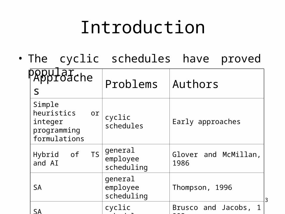
• The cyclic schedules have proved popular.

Approaches Problems AuthorsSimple heuristics or integer programming formulations

cyclic schedules Early approaches

Hybrid of TS and AIgeneral employee scheduling

Glover and McMillan, 1986

SAgeneral employee scheduling

Thompson, 1996

SA cyclic schedules Brusco and Jacobs, 1993

Knowledge based approaches

rostering airline ground crews and scheduling hospital doctors

Chow and Hui, 1993

Gierl et al., 1993

(suggestion)

4

Introduction

• In this case the objectives – To produce weekly schedules which meet

strict constraints on the numbers of nurses of different grades on duty at different times.

– This problem somewhat different from those in which the objectives are to minimize actual monetary costs.

5

The problem

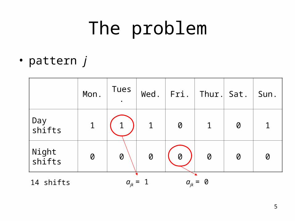
• pattern j

Mon. Tues. Wed. Fri. Thur. Sat. Sun.

Day shifts 1 1 1 0 1 0 1

Night shifts 0 0 0 0 0 0 0

14 shifts ajk = 1 ajk = 0

6

The problem

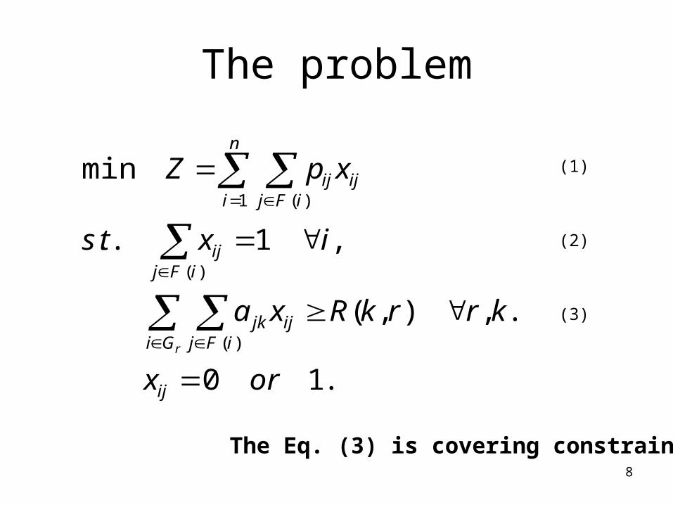
• Variable definition

xij

if nurse i works pattern j then xij = 1

Otherwise xij = 0

pij The penalty associated with nurse i working pattern j.

F(i) The set of patterns feasible for nurse i.

ajkif pattern j covers shift k then ajk = 1

Gr The set of nurses of grade-band r or above.

R(k,r) The minimum acceptable number of nurses of grade r or above for shift k.

7

The problem

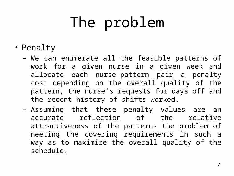
• Penalty– We can enumerate all the feasible patterns of work for

a given nurse in a given week and allocate each nurse-pattern pair a penalty cost depending on the overall quality of the pattern, the nurse’s requests for days off and the recent history of shifts worked.

– Assuming that these penalty values are an accurate reflection of the relative attractiveness of the patterns the problem of meeting the covering requirements in such a way as to maximize the overall quality of the schedule.

8

The problem

.10

.,),(

,1..

min

)(

)(

1 )(

　　　　　

　　　　

　　　

　

orx

krrkRxa

ixts

xpZ

ij

Gi iFjijjk

iFjij

n

i iFjijij

r

(1)

(2)

(3)

The Eq. (3) is covering constraint.

9

The local search framework (Neighborhood)

• The problem has two natural neighborhoods.① Involves moving from schedule to schedule by

changing the shift pattern of a single nurse by a single shift. This neighborhood would not enable the search to move

directly from one type of pattern to the other.

② This second neighborhood was selected as the basis for all moves and will be referred to throughout as the standard neighborhood. To overcome the first neighborhood, either the solution

space would need to be extended.

10

The local search framework (Handling the covering constraint)

• In a situation where all nurses work full-time and each nurse is available for all full-time shift patterns.– Feasible solutions satisfying constraints (2) and (3) is

easily.

• Once part-timers and infeasible patterns are incorporated, simply finding a feasible solution becomes more difficult.

• It was therefore decided to incorporate the search for feasible solutions into the main search process.

11

The local search framework (Handling the covering constraint)

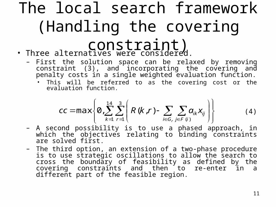
• Three alternatives were considered.– First the solution space can be relaxed by removing constraint

(3), and incorporating the covering and penalty costs in a single weighted evaluation function.

• This will be referred to as the covering cost or the evaluation function.

– A second possibility is to use a phased approach, in which the objectives relating to binding constraints are solved first.

– The third option, an extension of a two-phase procedure is to use strategic oscillations to allow the search to cross the boundary of feasibility as defined by the covering constraints and then to re-enter in a different part of the feasible region.

14

1

3

1 )(

),(,0maxk r Gi iFj

ijik

r

xarkRcc (4)

12

Obtaining a feasible solution with phase 1 (standard neighborhood)

• Phase 1 starts with a randomly generated solution and randomly selects moves using the standard neighborhood.– The candidate list is restricted to moves which

decrease the covering cost and do not increase the penalty cost.

– The first feasible candidate sampled is accepted.

• Any solution partitions the nurses into two sets:– Those working days.– Those working nights.

13


• Once a local optimum has been reach, moving a single nurse from one type to another usually involves a significant increase in covering cost.

Tt The set of shift patterns of type t.

Nt(i)The number of shifts in a pattern of type t worked by nurse i.

QtrThe total number of shifts of type t required for grade-band r.

r

t

GiTjiFj

trijt QxiN)(

)( (5)

14


• Such solutions will be referred to as unbalanced.– They can be corrected by a standard neighborhood move, which

moves a nurse who is not working a type t pattern to a type t pattern.

– The candidate list is restricted to moves which do this and the best move according to the covering cost is chosen.

• Local optima which are not unbalanced also occur frequently.– Examination of these solutions indicated that they were

surrounded by many zero-cost and small uphill moves.– A more intelligent approach of actively generating improving

chains of moves was chosen.

15

Obtaining a feasible solution with phase 1 (shift chain neighborhood)

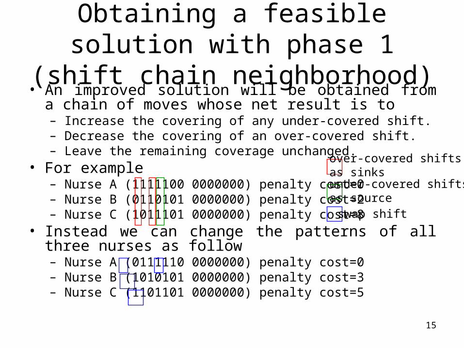
• An improved solution will be obtained from a chain of moves whose net result is to– Increase the covering of any under-covered shift.– Decrease the covering of an over-covered shift.– Leave the remaining coverage unchanged.

• For example– Nurse A (1111100 0000000) penalty cost=0– Nurse B (0110101 0000000) penalty cost=2– Nurse C (1011101 0000000) penalty cost=8

• Instead we can change the patterns of all three nurses as follow– Nurse A (0111110 0000000) penalty cost=0– Nurse B (1010101 0000000) penalty cost=3– Nurse C (1101101 0000000) penalty cost=5

over-covered shiftsas sinks under-covered shiftsas sourceswap shift

16


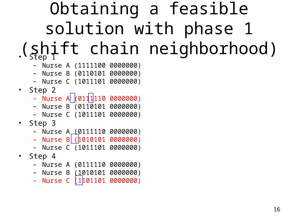
• Step 1– Nurse A (1111100 0000000)– Nurse B (0110101 0000000)– Nurse C (1011101 0000000)




17


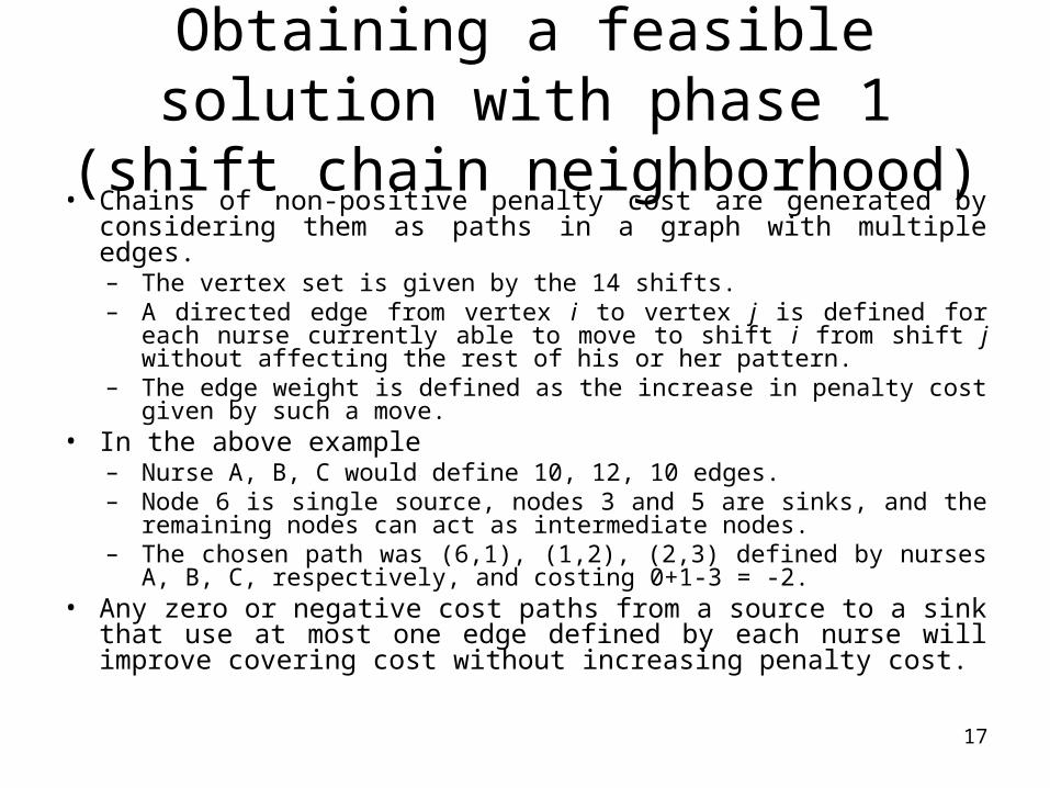
• Chains of non-positive penalty cost are generated by considering them as paths in a graph with multiple edges.– The vertex set is given by the 14 shifts.– A directed edge from vertex i to vertex j is defined for each nurse

currently able to move to shift i from shift j without affecting the rest of his or her pattern.

– The edge weight is defined as the increase in penalty cost given by such a move.

• In the above example– Nurse A, B, C would define 10, 12, 10 edges.– Node 6 is single source, nodes 3 and 5 are sinks, and the remaining

nodes can act as intermediate nodes.– The chosen path was (6,1), (1,2), (2,3) defined by nurses A, B, C,

respectively, and costing 0+1-3 = -2.• Any zero or negative cost paths from a source to a sink that use at

most one edge defined by each nurse will improve covering cost without increasing penalty cost.

18


• Using a depth first search (DFS) with the nodes ordered randomly to avoid built in bias until either a suitable path has been found or the search tree is exhausted.– The fourteen vertex graph can be regarded as

two disjoint graphs of seven vertices.– For a particular set of sources and sinks the

tree therefore has a maximum depth of five intermediate search nodes.

19

Obtaining a feasible solution with phase 1 (nurse chain

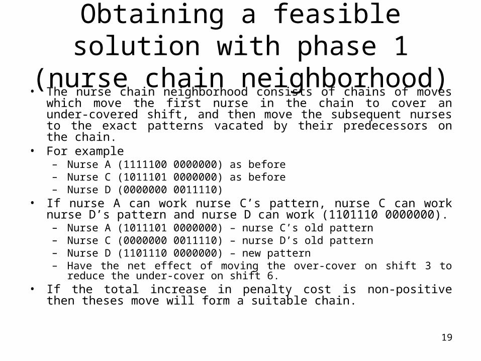
neighborhood)• The nurse chain neighborhood consists of chains of moves which move the

first nurse in the chain to cover an under-covered shift, and then move the subsequent nurses to the exact patterns vacated by their predecessors on the chain.

• For example– Nurse A (1111100 0000000) as before– Nurse C (1011101 0000000) as before– Nurse D (0000000 0011110)

• If nurse A can work nurse C’s pattern, nurse C can work nurse D’s pattern and nurse D can work (1101110 0000000).

– Nurse A (1011101 0000000) – nurse C’s old pattern– Nurse C (0000000 0011110) – nurse D’s old pattern– Nurse D (1101110 0000000) – new pattern– Have the net effect of moving the over-cover on shift 3 to reduce the under-cover

on shift 6.• If the total increase in penalty cost is non-positive then theses move will

form a suitable chain.

20

Obtaining a feasible solution with phase 1 (nurse chain

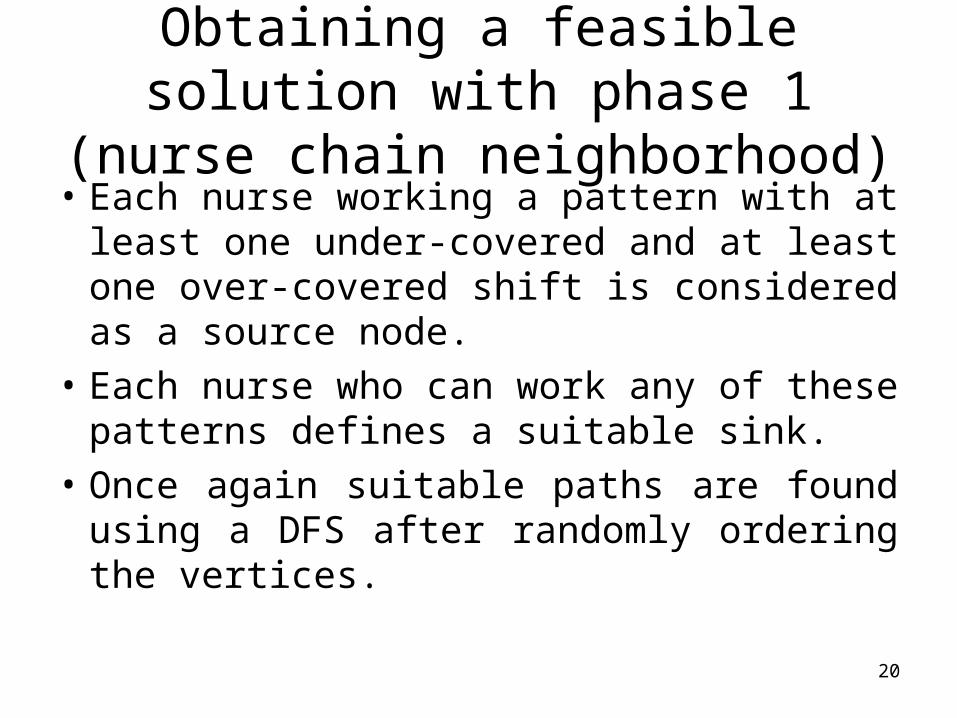
neighborhood)• Each nurse working a pattern with at least

one under-covered and at least one over-covered shift is considered as a source node.

• Each nurse who can work any of these patterns defines a suitable sink.

• Once again suitable paths are found using a DFS after randomly ordering the vertices.

21

The full phase 1 strategy

• Both chain neighborhoods are used aggressively to decrease covering cost without increasing penalty cost.

• The moves are attempted in order.– If the move is accepted the pointer returns to the top of the list.– Otherwise the next move is attempted.

22

Reducing penalty cost – phases 2 and3

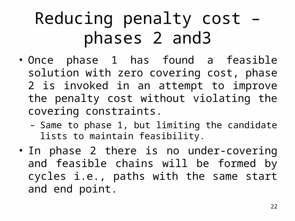
• Once phase 1 has found a feasible solution with zero covering cost, phase 2 is invoked in an attempt to improve the penalty cost without violating the covering constraints.– Same to phase 1, but limiting the candidate lists to

maintain feasibility.

• In phase 2 there is no under-covering and feasible chains will be formed by cycles i.e., paths with the same start and end point.

23

Reducing penalty cost – phases 2 and3

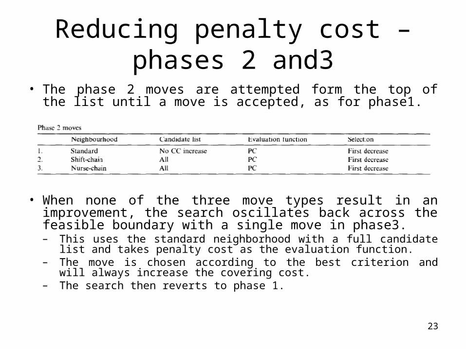
• The phase 2 moves are attempted form the top of the list until a move is accepted, as for phase1.

• When none of the three move types result in an improvement, the search oscillates back across the feasible boundary with a single move in phase3.– This uses the standard neighborhood with a full candidate list

and takes penalty cost as the evaluation function.– The move is chosen according to the best criterion and will

always increase the covering cost.– The search then reverts to phase 1.

24

An influential attribute

• There appeared to be certain data characteristics which lead to very variable results.– When there were just enough nurses to meet

overall covering requirements and the work force contained small numbers of nurses contracted to work four days or three nights and three days or three nights.

– When the covering constraints were slack.

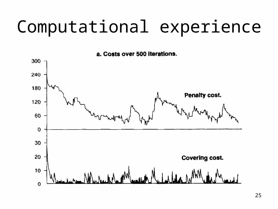
25

Computational experience

26


27


28

Conclusions

• One of this paper was to show how and why each of these ingredients was selected to gradually build an algorithm able to match the quality of solutions produced by a human expert.

1 nurse scheduling with tabu search and strategic oscillation jia-xian zhu

Documents