1

Computational Methods II(Elliptic)

Dr. Farzad Ismail

School of Aerospace and Mechanical EngineeringUniversiti Sains Malaysia

Nibong Tebal 14300 Pulau Pinang

Week 4- Lecture 1 and 2

2

Overview

We already know the nature of hyperbolic and parabolic PDE’s.

Now we will focus on elliptic PDE.

The elliptic PDE is a type of PDE for solving incompressible flow.

3

Overview (cont’d)

Elliptic PDE’s are always smooth

Easier to obtain accurate solutions compared to hyperbolic problems, the challenge is in getting solutions efficiently.

Unlike hyperbolic and parabolic problems, information is transmitted everywhere

4

Overview (cont’d)

The model problem that will be discussed is

Note that the problem is now 2D but with no time dependence

Laplace Equation

Poisson Eqn

5

Overview (cont’d)

6

Overview (cont’d)

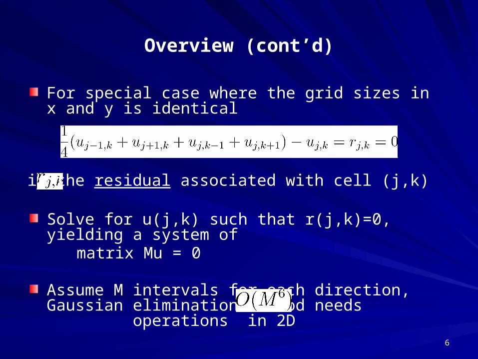
For special case where the grid sizes in x and y is identical

Solve for u(j,k) such that r(j,k)=0, yielding a system of matrix Mu = 0

Assume M intervals for each direction, Gaussian elimination method needs operations in 2D

is the residual associated with cell (j,k)

7

Iteration Method

Solving it directly is to expensive, usually an iteration method is employed.

The simplest iteration method is the point Jacobi method – based on solving the steady state of parabolic pde

Solve iteratively for until

8

Iteration Method (cont’d)

The superscript n denotes pseudo-time, not physical time

ω is the relaxation factor, analogous to μ

The first thought is to achieve steady-state as quickly as possible, hence choosing a largest ω consistent with stability

Not a good idea since we need to know what is the best choice for ω

9

Typical Residual Plot

10

Residual Pattern

Plot of convergence history

Has three distinct phases

First phase, the residual decays very rapidly

Second phase decays linearly on the log-plot (or exponentially in real plot)

Third phase is ‘noise’, since randomness has set in - after a while residuals become so small that they are of the order of round-off errors

11

Residual Pattern (cont’d)

Sometimes the residual plot would ‘hang’ up

Usually due to a ‘bug’ in the code

To save time, apply a ‘stopping’ criterion to residual

But not easy to do so, need to understand errors

12

Analyzing the Errors

We want know how the iteration errors decay.

Expand the solution as

The first term on the RHS is the solution after infinite number of iterations

The second term on the RHS is the error between the solution at iterative level n and after infinite iterations

Get the best solution if error is removed

13

Analyzing the Errors (cont’d)

Substitute the error relation into the iteration method.

Converge solution gives zero residual, hence

Iterations for error

14

Analyzing the Errors (cont’d)

Shows that error itself follow an evolutionary pattern

This is true for all elliptic problems

Remarkably, we can determine how the error would behave even if we do not know the solution

15

Analyzing the Errors using VA

In 2D, von Neumann analysis (VA)

Insert this into the error equation

Yields the amplification factor for the errors

16

Amplification factor for Point Jacobi Method

What does the figure tell you ???

17

G for Errors using Point Jacobi (cont’d)

The plot shows how the errors decay for various error modes (in terms of sines and cosines)

Consider 1D situation – let there be M+1 points on a line giving M intervals. The errors can be expressed as

where m = 1,2, .., M-1

18

Error Modes for M=8

Seven possible error modes on a 1D mesh with eight intervals – Lowest to highest frequencies.

19

Error Modes Analysis M=8

Any numbers satisfying f(0)=f(M)=0 can be represented as

This is a discrete Fourier Transform

In 1D, need only to consider the following set of discrete frequencies (lowest to highest)

20

2D situation

Consider 2D situation – let there be M+1 and N+1 points, giving M and N intervals in x and y directions

where m = 1,2, .., M-1. n=1,2,.. N-1.

Assume M=N, the highest and lowest frequencies correspond to

21

Discrete G versus z

- Each point corresponds to discrete error modes, each error mode decays differently even for samerelaxation factor

- Note ZL = -ZR

22

Decay of Error Modes

In eliminating the errors, we do not care the sign of amplitude, just the magnitude of it – want g as small as possible

If 0 < |g| < 1 for ALL error modes, then we could say that we eventually will remove all the iteration errors and hence a steady state solution will be obtained.

However, the errors will be removed at different rates, with modes corresponding to the largest |g| (convergence rate) will be most difficult to be removed- dominant error mode

23

Decay of Error Modes (cont’d)

For ω=0.6, it is clear that ZR (lowest frequency) is the dominant error mode

Increasing ω, will decrease g until ω=1 – both lowest and highest frequency modes become dominant

Beyond ω > 1, ZL (highest frequency) modes become more dominant and |g| deteriorates.

24

Computational Cost

Recall for direct method (Gaussian Elimination) requires in 2D and in 3D.

Using point Jacobi iteration methods costs in 2D and in 3D.

Can this be improved? Let say by one order magnitude?

25

Gauss Seidel

- When visiting node (j,k) at time level n+1, can use information of nodes (j,k-1) at time level n and (j-1, k) at n+1 (square nodes)

- This is Gauss-Seidel method

26

SOR Method

Coupling Gauss-Seidel with point Jacobi gives Successive Over- Relaxation (SOR) method

It can be shown that using VA, the convergence rate

Only consider real z such that

27

G versus z for SOR

- Note now z = [0,2]

- Similar to Point Jacobi for ω less than or equal to 1

- But improved convergence rate for ω > 1 (1.16, 1.36, 1.64, 1.81 ) -> STILL LOWEST FREQUENCY MODE IS DOMINANT

28

Discussion of Low Frequency Modes

We have seen that the low frequency modes are most difficult to get rid of for Point Jacobi and SOR methods

Moderate to high frequency modes are usually much easier to be removed.

This is the general behavior for almost all methods in solving elliptic PDE

Need to think out of the box

29

Multigrid (Brandt)

Use a hierachy of different grid sizes to solve the elliptic PDE –splitting the error modes

The low frequency error modes on a fine grid will appear as high frequency modes on a coarser grid.

Hence easier to be removed

But there is a problem with coarse grids.

30

Multigrid Mesh

- An 8 x 8 grid superimposed with 4 x 4 + 2 x 2 grid

31

Multigrid (cont’d)

Although coarse grids will remove the error modes quickly, but it will converge to an inaccurate solution

Need to combine the accuracy of fine grids with the fast convergence on coarse grids

As long as there are significant error modes in fine grid, coarse grid must be kept to work

Fine grids must ‘tell’ the coarse grids the dominant error modes and ask ‘advice’ on how to remove them – restriction operator

32

Multigrid (cont’d)

Coarse grids will give information on how to remove the dominant error modes to fine grids and ask for ‘advice’ regarding accuracy- prolongation operator

Communication between coarse-fine grids is the key

In between, perform relaxation (solving the steady state equation)

33

Story

34

Multigrid V Cycle