07 logistic regression - cs.tufts.edu

Logistic Regression

1

Tufts COMP 135: Introduction to Machine Learninghttps://www.cs.tufts.edu/comp/135/2019s/

Many slides attributable to:Erik Sudderth (UCI)Finale Doshi-Velez (Harvard)James, Witten, Hastie, Tibshirani (ISL/ESL books)

Prof. Mike Hughes

https://www.cs.tufts.edu/comp/135/2019s/

Logistics

• Waitlist: We have room, contact me ASAP

• HW3 due Wed• Please annotate pages in Gradescope!• Remember: Turn in on time!

• Recitation tonight (730-830pm, Room 111B)• Practical binary classifiers in Python with sklearn• Numerical issues and how to address them

2Mike Hughes - Tufts COMP 135 - Spring 2019

Objectives:Logistic Regression Unit

Refresher: “taste” of 3 Methods• Logistic Regression, k-NN, Decision Trees

Logistic Regression: A Probabilistic Classifier• 3 views on why we optimize log loss

• Upper bound error rate• Minimize (cross) entropy• Maximize (log) likelihood

• Computing gradients• Training via gradient descent


What will we learn?


SupervisedLearning

Unsupervised Learning

Reinforcement Learning

Data, Label PairsPerformance

measureTask

data x

labely

{xn, yn}Nn=1

Training

Prediction

Evaluation


y

x2

x1

is a binary variable (red or blue)

SupervisedLearning

binary classification

Unsupervised Learning

Reinforcement Learning

Task: Binary Classification

Example: Hotdog or Not


https://www.theverge.com/tldr/2017/5/14/15639784/hbo-silicon-valley-not-hotdog-app-download

https://www.theverge.com/tldr/2017/5/14/15639784/hbo-silicon-valley-not-hotdog-app-download

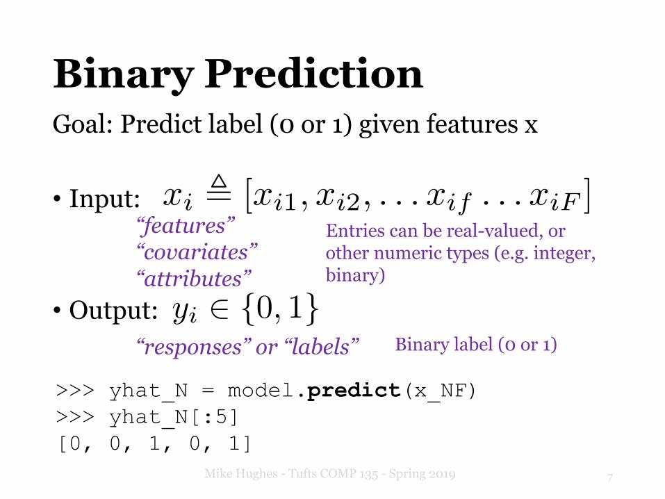
>>> yhat_N = model.predict(x_NF)>>> yhat_N[:5][0, 0, 1, 0, 1]

Binary PredictionGoal: Predict label (0 or 1) given features x

• Input:

• Output:


xi , [xi1, xi2, . . . xif . . . xiF ]Entries can be real-valued, or other numeric types (e.g. integer, binary)

Binary label (0 or 1)

“features”“covariates”“attributes”

“responses” or “labels”yi 2 {0, 1}

>>> yproba_N2 = model.predict_proba(x_NF)>>> yproba1_N = model.predict_proba(x_NF)[:,1]>>> yproba1_N[:5][0.143, 0.432, 0.523, 0.003, 0.994]

Probability PredictionGoal: Predict probability of label given features

• Input:

• Output:


xi , [xi1, xi2, . . . xif . . . xiF ]Entries can be real-valued, or other numeric types (e.g. integer, binary)

“features”“covariates”“attributes”

“probability”pi , p(Yi = 1|xi) Value between 0 and 1

e.g. 0.001, 0.513, 0.987

Decision Tree Classifier


Leaves make binary predictions! (but can be made probabilistic)

Goal: Does patient have heart disease?


Decision Tree ClassifierParameters:

- at each internal node: x variable id and threshold- at each leaf: probability of positive y label

Prediction:- identify rectangular region for input x - predict: most common y value in region- predict_proba: report fraction of each label in regtion

Training:- minimize error on training set- often, use greedy heuristics

Decision Tree: Predicted Probas


Pretty flexible!

Function is piecewise constantand axis-aligned

K nearest neighbor classifier


Parameters:K : number of neighbors

Prediction:- find K “nearest” training vectors to input x- predict: vote most common y in neighborhood- predict_proba: report fraction of labels

Training:none needed (use training data as lookup table)

KNN: Predicted Probas


Very flexible!

Function is piecewise constant

Logistic Regression classifierParameters:

Prediction:

Training:find weights and bias that minimize error


w = [w1, w2, . . . wf . . . wF ]b

weight vector

bias scalar

p(yi = 1|xi) , sigmoid

0

@FX

f=1

wfxif + b

1

Ap(xi, w, b) =

Logistic Sigmoid Function


sigmoid(z) =1

1 + e�z

Goal: Transform real values into probabilitiespr

obab

ility

Logistic Regression: Training


Optimization: Minimize total log loss on train set

min

w,b

NX

n=1

log loss(yn, p(xn, w, b))

Algorithm: Gradient descent

Today!

Avoid overfitting: Use L2 or L1 penalty on weights

Logistic Regr: Predicted Probas


Function ismonotonically increasing in one direction

Decision boundarieswill be linear

Summary of Methods


Function classflexibility

Knobs to tune Interpret?

LogisticRegression

Linear L2/L1 penalty on weights Inspect weights

Decision TreeClassifier

Axis-alignedPiecewise constant

Max. depthMin. leaf sizeGoal criteria

Inspecttree

K Nearest NeighborsClassifier

Piecewise constant Number of NeighborsDistance metricHow neighbors vote

Inspect neighbors

Optimization ObjectiveWhy minimize log loss?An upper bound justification


Log loss upper bounds error rate


log loss(y, p) = �y log p� (1� y) log(1� p)

Plot assumes:

- True label is 1

- Threshold is 0.5

- Log base 2

error(y, y) =

(1 if y 6= y

0 if y = y

Optimization ObjectiveWhy minimize log loss?An information-theory justification


Entropy of Binary Random Var.


Goal: Entropy of a distribution captures the amount of uncertainty

entropy(X) = �p(X = 1) log2 p(X = 1)� p(X = 0) log2 p(X = 0)

Log base 2: Units are “bits”Log base e: Units are “nats”

1 bit of information is always needed to represent a binary variable X

Entropy tells us how much of this one bit is uncertain

Entropy of Binary Random Var.


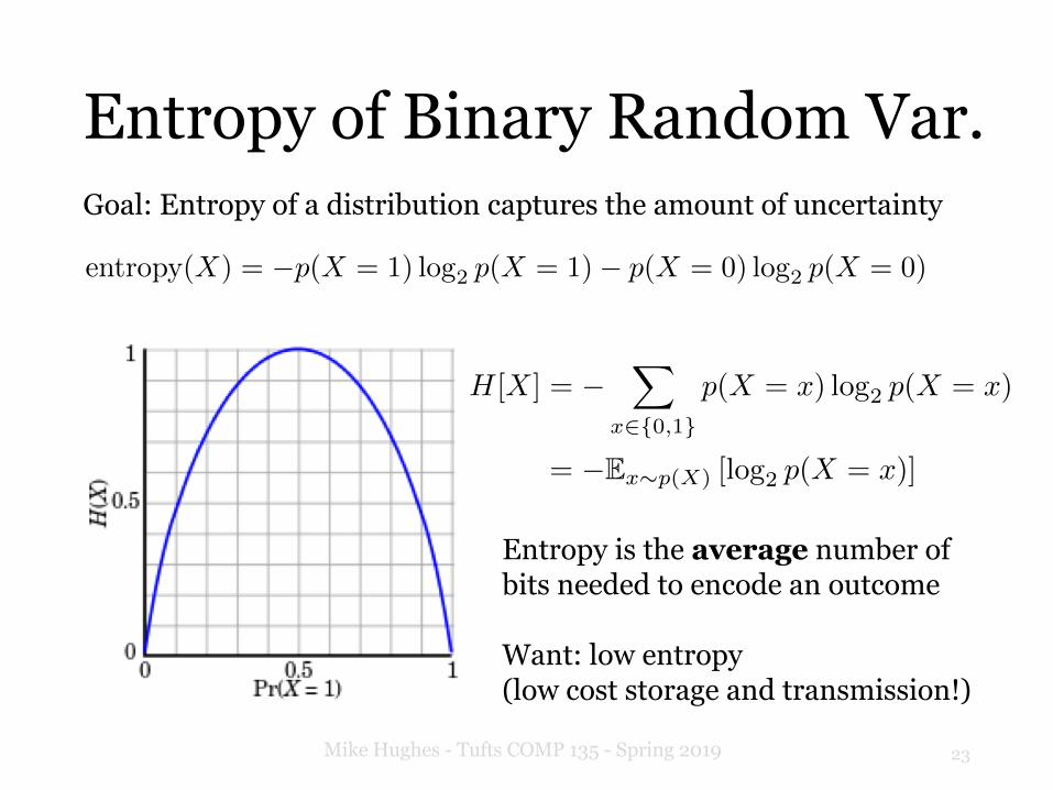
Goal: Entropy of a distribution captures the amount of uncertainty

entropy(X) = �p(X = 1) log2 p(X = 1)� p(X = 0) log2 p(X = 0)

H[X] = �X

x2{0,1}

p(X = x) log2 p(X = x)

= �Ex⇠p(X) [log2 p(X = x)]

Entropy is the average number ofbits needed to encode an outcome

Want: low entropy(low cost storage and transmission!)

Cross Entropy


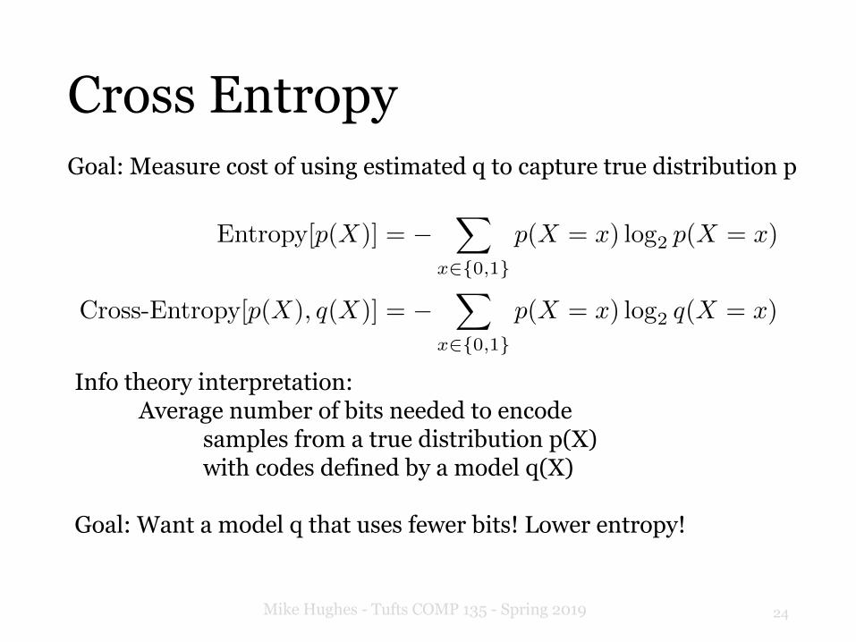
Goal: Measure cost of using estimated q to capture true distribution p

Entropy[p(X)] = �X

x2{0,1}

p(X = x) log2 p(X = x)

Cross-Entropy[p(X), q(X)] = �X

x2{0,1}

p(X = x) log2 q(X = x)

Info theory interpretation: Average number of bits needed to encode

samples from a true distribution p(X)with codes defined by a model q(X)

Goal: Want a model q that uses fewer bits! Lower entropy!

Log loss is cross entropy!


Let our “true” distribution p(Y) be empirical distribution of labels in the training set

Let our “model” distribution q(Y) be the estimated probabilities from logistic regression

Cross-Entropy[p(Y ), q(Y )] = Ey⇠p(Y ) [� log q(Y = y)]

=

1

N

NX

n=1

�yn log pn � (1� yn) log(1� pn)

Same as the “log loss”!

Info Theory Justification for log loss: Want to set logistic regression weights to provide best encoding of the training data’s label distribution

The log loss metric


Log loss (aka “binary cross entropy”)

log loss(y, p) = �y log p� (1� y) log(1� p)

from sklearn.metrics import log_loss

Advantages:• smooth• easy to take

derivatives!

Lower is better!


Optimization ObjectiveWhy minimize log loss?A probabilistic justification

Likelihood of labels under LR


We can write the probability for each outcome of Y as:

p(Yi = 1|xi) = sigmoid(w

Txi + b)

p(Yi = 0|xi) = 1� sigmoid(w

Txi + b)

We can write the probability mass function of Y as:

p(Yi = yi|xi) =⇥�(wT

xi + b)⇤yi

⇥1� �(wT

xi + b)⇤1�yi

Interpret: p(y | x) is the “likelihood” of label y given input features xGoal: Fit model to make the training data as likely as possible

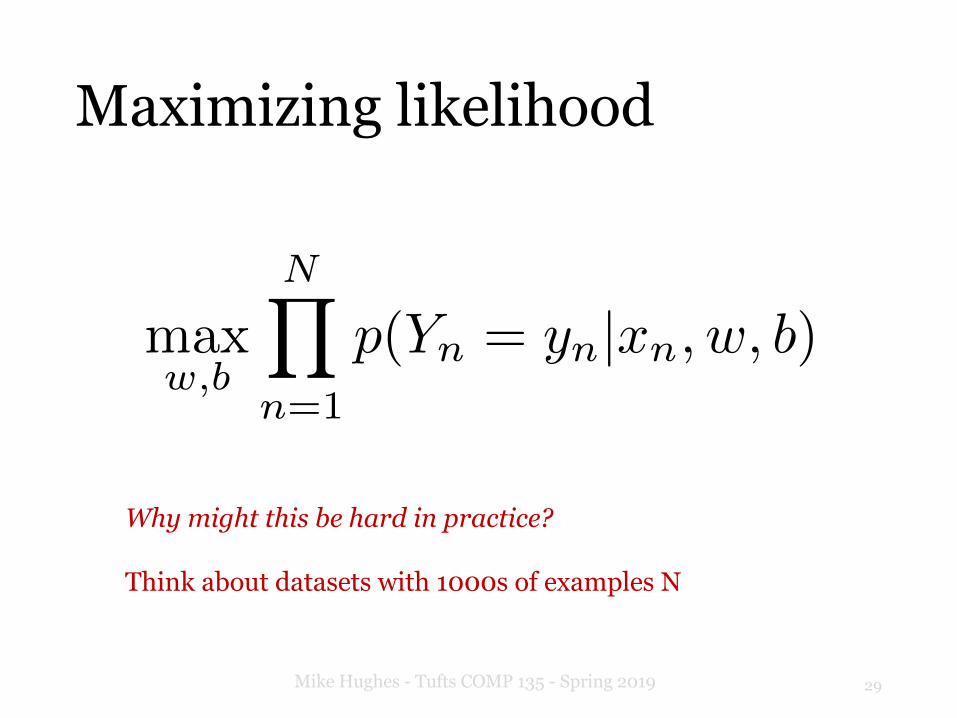
Maximizing likelihood


max

w,b

NY

n=1

p(Yn = yn|xn, w, b)

Why might this be hard in practice?

Think about datasets with 1000s of examples N

Maximizing log likelihood


The logarithm (with any base) is a monotonic transform

a > b implies log (a) > log (b)

Thus, the following are equivalent problems

w

⇤, b

⇤= argmax

w,b

NY

n=1

p(Yn = yn|xn, w, b)

w

⇤, b

⇤= argmax

w,blog

"NY

n=1

p(Yn = yn|xn, w, b)

#

Log likelihood for LR


We can write the probability mass function of Y as:

Our training objective is to maximize log likelihood

p(Yi = yi|xi) =⇥�(wT

xi + b)⇤yi

⇥1� �(wT

xi + b)⇤1�yi

Pair Exercise: Simplify the training objective J(w,b)!

Can you recover a familiar form?

w

⇤, b

⇤= argmax

w,b

NY

n=1

p(Yn = yn|xn, w, b)

w

⇤, b

⇤= argmax

w,blog

"NY

n=1

p(Yn = yn|xn, w, b)

#

J(w, b)

Minimize negative log likelihood

Two equivalent optimization problems:


w

⇤, b

⇤= argmax

w,b

NX

n=1

log p(Yn = yn|xn, w, b)

w

⇤, b

⇤= argmin

w,b�

NX

n=1

log p(Yn = yn|xn, w, b)

Summary of “Likelihood interpretation”

• LR defines a probabilistic model for Y given x• We want to maximize probability of training

data (the “likelihood”) under this model • We can show that an another optimization

problem (”maximize log likelihood”) is easier numerically but produces the same optimal values for weights and bias• Turns out, minimizing log loss is precisely the

same thing as minimizing negative loglikelihood


Computing gradients


Simplified LR notation

• Feature vector with first entry constant

• Weight vector (first entry is the “bias”)

• “Score” value z (real number, -inf to +inf)


w = [w0 w1 w2 . . . wF ]

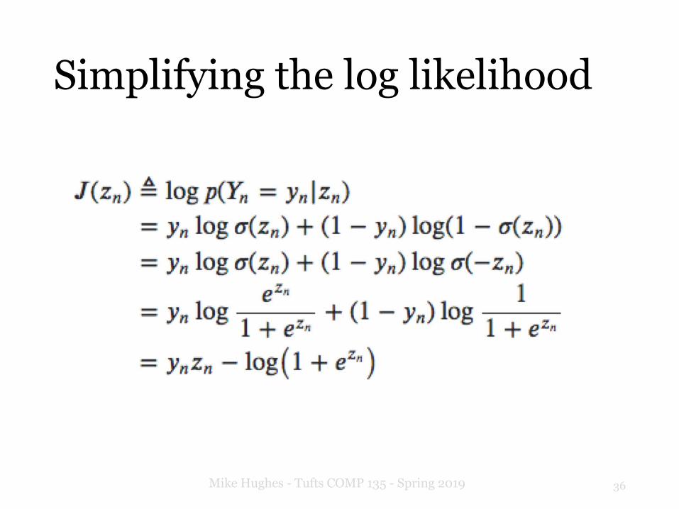
Simplifying the log likelihood


Gradient of the log likelihood


J(zn(w)) = ynzn � log(1 + ezn)

d

dwfJ(zn(w)) =

d

dznJ(zn) ·

d

dwfz(w)J(zn(w)) = ynzn � log(1 + ezn)

d

dwfJ(zn(w)) =

d

dznJ(zn) ·

d

dwfz(w)

= (yn � �(zn))xnfSimplifying yields:

Log likelihood

Gradient w.r.t. weight on feature f

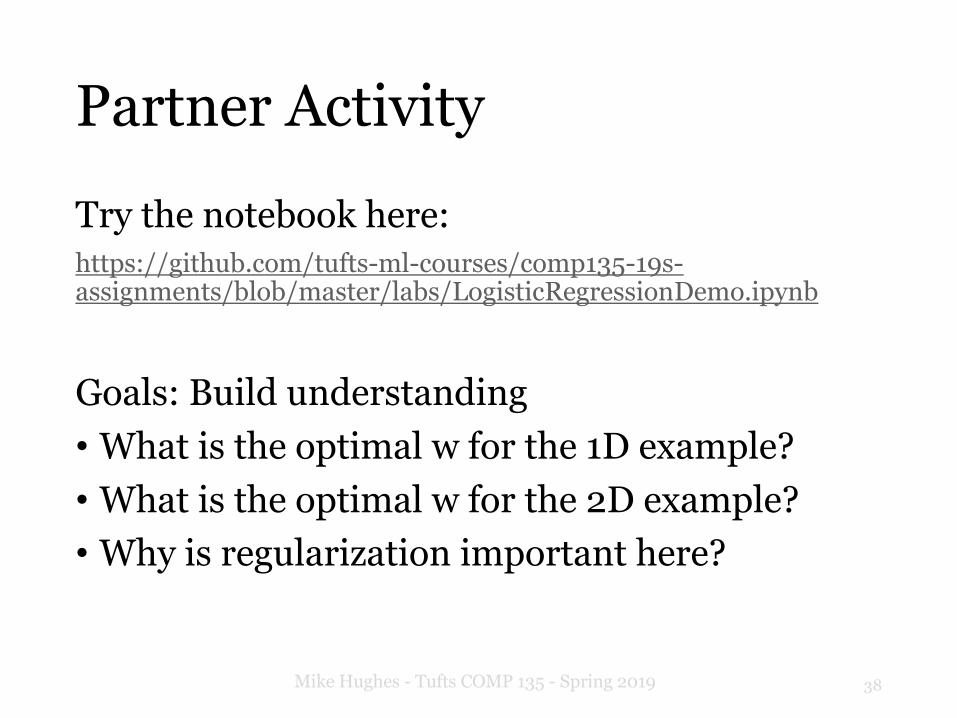
Partner Activity

Try the notebook here:https://github.com/tufts-ml-courses/comp135-19s-assignments/blob/master/labs/LogisticRegressionDemo.ipynb

Goals: Build understanding• What is the optimal w for the 1D example?• What is the optimal w for the 2D example?• Why is regularization important here?


https://github.com/tufts-ml-courses/comp135-19s-assignments/blob/master/labs/LogisticRegressionDemo.ipynb

STOP: End of class 2/11


Gradient descent for LR


Gradient descent for L2 penalized LR


Start with !" = 0,&"" = 0, step size -for . = 0,… , (1 − 1)

!567 = !5 − s 89 !5, &"5 − :!5

&"567 = &"5 − s 89 !5, &"5

if ; !567, &"567 − ; !5, &"5 < =break

return !>, &">

min!,AB

−∑D log H ID JD;!,&") +:2 ! N

N

J(w,w0)

Will gradient descent always find same solution?


Log loss is convex!


Intuition: 1D minimization


!(#)

#

!(#)

## #

Log likelihood vs iterations


If step size is too small


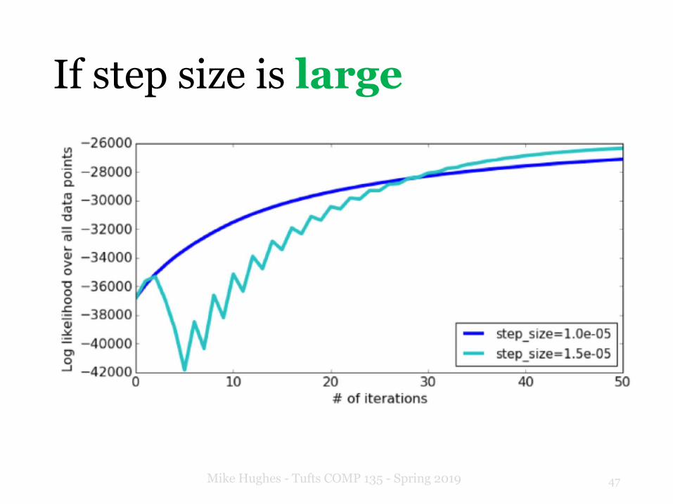
If step size is large


If step size is too large


If step size is way too large


Rule for picking step sizes• Never try just one!• Try several values (exponentially spaced) until

• Find one clearly too small• Find one clearly too large (oscillation / divergence)

• Always make trace plots!• Show the loss, norm of gradient, and parameters

• Smarter choices for step size:• Decaying methods• Search methods• Adaptive methods


Decaying step sizes

• Decay over iterations


Searching for good step sizes

• Line Searchscipy.optimize.line_search


07 logistic regression - cs.tufts.edu

Documents