` Research Division Federal Reserve Bank of St. Louis Working Paper Series

Do European Capital Flows Comove?

Silvio Contessi and

Pierangelo De Pace

Working Paper 2008-042B http://research.stlouisfed.org/wp/2008/2008-042.pdf

November 2008 Revised May 2009

FEDERAL RESERVE BANK OF ST. LOUIS Research Division

P.O. Box 442 St. Louis, MO 63166

______________________________________________________________________________________

The views expressed are those of the individual authors and do not necessarily reflect official positions of the Federal Reserve Bank of St. Louis, the Federal Reserve System, or the Board of Governors.

Federal Reserve Bank of St. Louis Working Papers are preliminary materials circulated to stimulate discussion and critical comment. References in publications to Federal Reserve Bank of St. Louis Working Papers (other than an acknowledgment that the writer has had access to unpublished material) should be cleared with the author or authors.

Do European Capital Flows Comove?∗

Silvio Contessi

Federal Reserve Bank of St. Louis

Pierangelo De Pace

Johns Hopkins University

March 2009

Abstract

We study the cross-section correlations of net, total, and disaggregated capital flows for the major

source and recipient European Union countries. We seek evidence of changes in these correlations

since the introduction of the euro to understand whether the European Union can be considered a

unique entity with regard to its international capital flows. We make use of Ng’s (2006) “uniform

spacing” methodology to rank cross-section correlations and shed light on potential common factors

driving international capital flows. We find that a common factor structure is suitable for equity flows

disaggregated by sign but not for net and total flows. We only find mixed evidence that correlations

between types of flows have changed since the introduction of the euro.

JEL Classification: F32, F34, F36

Keywords: capital flows volatility, foreign direct investment, foreign portfolio investment,

uniform spacings, group effects

∗We thank Serena Ng for providing the MATLAB codes, Ariel Weinberger for capable research assistance,Andrew Hughes Hallett for helpful discussion, and the participants in The Implications of European Integrationconference organized by the Federal Reserve Bank of St. Louis for their comments. Silvio Contessi: Federal ReserveBank of St. Louis, Research Division, P.O. Box 442, St. Louis MO 63166-0442. Pierangelo De Pace (correspondingauthor): Johns Hopkins University, 3400 N. Charles Street, Baltimore MD 21218, pierangelo.depace@jhu.edu. Theviews expressed are those of the authors and do not represent official positions of the Federal Reserve Bank of St.Louis, the Board of Governors, or the Federal Reserve System.

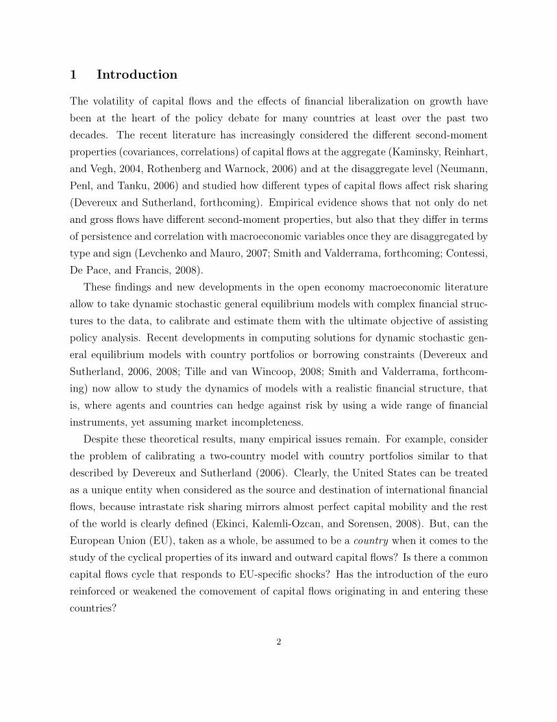
1 Introduction

The volatility of capital flows and the effects of financial liberalization on growth have

been at the heart of the policy debate for many countries at least over the past two

decades. The recent literature has increasingly considered the different second-moment

properties (covariances, correlations) of capital flows at the aggregate (Kaminsky, Reinhart,

and Vegh, 2004, Rothenberg and Warnock, 2006) and at the disaggregate level (Neumann,

Penl, and Tanku, 2006) and studied how different types of capital flows affect risk sharing

(Devereux and Sutherland, forthcoming). Empirical evidence shows that not only do net

and gross flows have different second-moment properties, but also that they differ in terms

of persistence and correlation with macroeconomic variables once they are disaggregated by

type and sign (Levchenko and Mauro, 2007; Smith and Valderrama, forthcoming; Contessi,

De Pace, and Francis, 2008).

These findings and new developments in the open economy macroeconomic literature

allow to take dynamic stochastic general equilibrium models with complex financial struc-

tures to the data, to calibrate and estimate them with the ultimate objective of assisting

policy analysis. Recent developments in computing solutions for dynamic stochastic gen-

eral equilibrium models with country portfolios or borrowing constraints (Devereux and

Sutherland, 2006, 2008; Tille and van Wincoop, 2008; Smith and Valderrama, forthcom-

ing) now allow to study the dynamics of models with a realistic financial structure, that

is, where agents and countries can hedge against risk by using a wide range of financial

instruments, yet assuming market incompleteness.

Despite these theoretical results, many empirical issues remain. For example, consider

the problem of calibrating a two-country model with country portfolios similar to that

described by Devereux and Sutherland (2006). Clearly, the United States can be treated

as a unique entity when considered as the source and destination of international financial

flows, because intrastate risk sharing mirrors almost perfect capital mobility and the rest

of the world is clearly defined (Ekinci, Kalemli-Ozcan, and Sorensen, 2008). But, can the

European Union (EU), taken as a whole, be assumed to be a country when it comes to the

study of the cyclical properties of its inward and outward capital flows? Is there a common

capital flows cycle that responds to EU-specific shocks? Has the introduction of the euro

reinforced or weakened the comovement of capital flows originating in and entering these

countries?

2

In this paper we attempt to answer these questions. In the first part, we use Ng (2006)’s

“uniform spacings” method to determine whether the comovement of disaggregated capital

flows has increased with the introduction of the euro in 1999. Although the breakpoint

date could have been estimated, rather than exogenously imposed, we choose to use an

exogenous breakpoint that looks natural for European economies. In related research , we

show that the conditional variance of the cyclical component of individual capital flows

exhibits a structural break between the first quarter of 1998 and the second quarter of 1999

in most cases (Contessi, De Pace, and Francis, 2008).

We analyze disaggregated capital flows organized in 11 panels, assess the extent of

their cross-section correlation, and find that a common factor structure is suitable for

equity flows disaggregated by sign but not for net and total flows. Hence, as suggested

by recent theoretical contributions (Devereux and Sutherland, 2006, 2008; Tille and van

Wincoop, 2008), the analysis of countries’ gross assets and liabilities and their breakdown

into different types might be important when capital flows are interpreted as adjustments

to country portfolios.

In the second part of our paper, we examine changes in correlation between different

types of flows for each country over the two subperiods 1990-1998 and 1999-2006. We

measure these correlations and formally test for changes over the two subperiods using a

statistical approach originally suggested by Doyle and Faust (2005) and later revisited by

De Pace (2008). We find mixed evidence of significant changes and no systematic pattern.

The structure of the paper is as follows. Section 2 describes the data, Section 3 explains

the methodologies we use to detect the presence of common factors in European capital

flows and to test for correlation changes. In Section 4 we present the results, followed by

our conclusions in Section 5.

2 International Capital Flows

Most of the literature on international capital flows focuses on net flows, often defined as the

difference between aggregate inflows and outflows. Recent empirical contributions, such as

those of Lipsey (1999), Rothenberg and Warnock (2006), and Kose, Prasad, and Terrones

(forthcoming), have pointed out that disaggregated flows data contain relevant information

that helps understand aggregate net flows. In addition to how they are classified in the

balance of payments, the economic characteristics of each type of capital flow are quite

3

different. Transactions such as bank loans, government securities, bonds, and equity are

conducted and observed in markets populated by many buyers and sellers, standardized

contracts, and publicly available prices. On the contrary, foreign direct investment (FDI)

is the result of financial and industrial decisions that are internal to the firm, not market-

mediated. In the case of emerging economies, an empirical case for separately examining

inflows and outflows is made by Rothenberg and Warnock (2006), who look at gross flows

and show that about half of the observed sudden stops (retreat of global investors) are

actually episodes of sudden flight of local investors.

In two recent theoretical exceptions, Tille and van Wincoop (2008) and Devereux and

Sutherland (forthcoming) develop a novel solution for two-country DSGE models with

country portfolios and stress the importance of distinguishing between gross and net flows.

In a small open economy setting, Smith and Valderrama (forthcoming) discuss the cyclical

properties of different types of flows to a group of emerging countries using data recorded at

the quarterly frequency. Unlike previous open economy macroeconomic models that stylize

international financial linkages in terms of net foreign assets and the current account, these

papers consider the fact that the data show huge cross-country gross asset and liability

positions in assets whose value might change radically over short periods, even if the trade

balance barely moves (Lane and Milesi Ferretti, 2007). The size of such gross asset positions

suggests the need of understanding the determinants of portfolio choice and their effects

on macroeconomic dynamics. For example, fluctuations of the nominal exchange rate alter

capital gains and losses for gross positions, with potentially large effects on the value of

net foreign assets (depending on the composition of countries’ portfolios). However, they

do not necessarily imply changes in net export.

We interpret different types of capital flows as adjustments to country positions of FDI,

foreign portfolio investment (FPI), and debt stocks. We focus on quarterly data on capital

flows, disaggregated by sign and type. Complete series are available for the period 1990:Q1

through 2006:Q4 for the major countries in the EU (France, Germany, Italy, Finland, the

Netherlands, Portugal, Spain, the United Kingdom, and Sweden).1 International capital

flows are reported as assets (outflows) and liabilities (inflows), separately for each country.

We collect 11 panels organized as follows. (i) Inward foreign direct investment (iFDI) is

direct investment in the reporting economy, (ii) outward foreign direct investment (oFDI)

1Source: International Financial Statistics (IFS), published by the International Monetary Fund (IMF), various issues.

4

is direct investment abroad. Both types of investment include equity capital, reinvested

earnings, other capital, and financial derivatives associated with various intercompany

transactions with affiliated companies, as discussed in IMF (2007). Inward and outward

portfolio investment includes financial securities of any maturity, including corporate se-

curities, bonds, notes, and money market instruments other than those parts of direct

investment or reserve assets. Because IFS data combine debt and equity portfolio invest-

ment, we separate Equity Securities from Debt Securities. According to our definition,

(iii) inward (iFPI) and (iv) outward equity securities (oFPI) include only shares, stock

participation, and similar equity investments (e.g., American Depository Receipts and

Global Depository Receipts). Debt securities assets and liabilities include bonds, deben-

tures, notes, and money market or negotiable debt instruments. We combine these series

with other investment assets and liabilities (i.e., all the financial transactions not covered

in direct investment, portfolio investment, financial derivatives, or other assets, such as

trade credits, loans, transactions in currency and deposits, and other assets/liabilities).

We define these aggregates as (v) inward debt (iDebt) and (vi) outward debt (oDebt). To-

tal equity flows are calculated as equity securities plus foreign direct investment for both

inflows and outflows and labelled (vii) total equity liabilities (iEqu) and (viii) total equity

assets (oEqu). Total equity flows plus total debt flows are summed as (ix) total inflows

liabilities (iTot) and total outflows assets (oTot). The difference between oTot and iTot is

(xi) net outward flows (noTot). Table 1 summarizes the classification of capital flows.

We study the levels of the quarterly series of nominal capital flows. A few series exhibit

occurrences of negative values or zero entries. In some cases, negative values may be due to

either underreporting or large disinvestment; the latter is often caused by repatriation of

previous investment (for example, negative FDI inflows). Given the nature of our dataset,

using the log of capital flows to reduce the weight of observations with particularly large

quarter-specific values is not always viable, because some entries in the series may be

negative or zero. A semi-logarithmic transformation would deal with zero entries, but

would not solve the issue of negative observations. We use the solution described in Levy-

Yeyati, Panizza, and Stein (2007) and opt for the transformation

Flow∗t = sign (Flowt)× log (1 + |Flowt|) (1)

5

where Flowt can be any of the capital flow series previously described. This manipulation

of the data still allows the application of conventional filtering methods to the transformed

variables without distorting standard interpretations. We detrend the transformed capital

flow series using a standard Hodrick-Prescott filter.

3 The Econometric Framework

In this section, we briefly describe the theoretical framework developed in Ng (2006) to

test for cross-section correlations and briefly refer to De Pace (2008) for a formal test on

correlation changes based on bootstrap methods.

3.1 Cross-Section Correlations: Ng’s Uniform Spacings Methodology

We test for the significance of cross-section correlations in 11 panels of data on international

capital flows, organized by type and sign, and treated as previously described.

Our adoption of Ng’s (2006) methodology is motivated by the observation that the

majority of tests for cross-section correlation in panels of data are based on the null hy-

pothesis that all the units exhibit no correlation against the alternative hypothesis that

the correlation is different from zero for some units.2 Such statistical tests provide no

guidance on the assessment of the extent of correlation in the panel if the null is rejected.

On the contrary, the application of Ng (2006)’s uniform spacings methodology allows the

determination of whether at least some (not necessarily all) countries in the sample have

correlated capital flows. Furthermore, we can identify those countries clearly. Formally,

for the panel of a specific capital flow, let M be the number of countries in the sample

and T the number of time-series observations (quarters herein). The number of unique

elements above (or below) the diagonal of the sample correlation matrix is denoted by

N = M(M−1)2

.3 Let ρ = (|ρ̂1| , |ρ̂2| , ..., |ρ̂N |)′ be the vector of the absolute sample correla-

tion coefficients: the absolute values of the estimates of the population correlations in the

vector ρ = (ρ1, ρ2, ..., ρN)′. Then sort the elements in ρ from the smallest to the largest

in the ordered series(ρ[1:N ], ρ[2:N ], ..., ρ[N :N ]

)′. Finally, define φj = Φ

(√Tρ[j:N ]

), where

2An assessment of the extent of cross-section correlation in the errors has significant implications for estimation andinference. Andrews (2005) showed that ordinary least squares applied to cross-section data can be inconsistent unless theerrors, conditional on the common shock, are uncorrelated with the regressors.

3The application of the testing strategy requires the correlation coefficients to be ordered from the smallest to the largest.We do not directly test whether the sample correlations (jointly or individually) are zero. Instead, as we describe later, thegoal is to test whether the probability integral transformation of the ordered correlations, φj , is uniformly distributed.

6

Φ is the cumulative distribution function of a standard normal distribution.4 Given that

ρ[j:N ] ∈ [0, 1] ∀j, then φj ∈ [0.5, 1], from which Ng (2006) shows that the null hypothesis of

ρj = 0 is equivalent to the null of φj ∼ U (0.5, 1). The q-order uniform spacings are simply

defined as{(φj − φj−q

)}Nj=1

.5

We partition the N absolute sample correlations into two groups: S for small (con-

taining the smaller absolute correlations) and L for large (containing the larger absolute

correlations), with θ ∈ [0, 1] being the fraction of the sample contained in S. θ is estimated

through maximum likelihood using a standard breakpoint analysis. The S group has size

K̂, whereas the L group has size(N − K̂

). It may happen that the

(N − K̂

)correla-

tions in L are not statistically different from the K̂ correlations in S. In that case, the

strategy is to test whether the K̂ correlations in S are zero. If the small correlations are

statistically different from zero, then the correlations in L must also be different from zero

by construction. Ng (2006) proposes a standardized spacings variance-ratio (SV R) test

based on a statistic, SV R (η), that asymptotically follows a standard normal distribution

under the null of no correlation in the subsample of size η.6

The SV R test can be applied to the full sample, to S, or to L, with η = N , η =

K̂, or η =(N − K̂

), respectively. The SV R test is based on the spacings, which are

exchangeable. This fact implies that the test can be performed on any subset of the

ordered correlations. It can be shown that, if the data are uncorrelated, the φj all lie along

a straight line. This allows to use any partition of the full sample to test the slope. If the

uniformity hypothesis on the φj is rejected in S, testing whether the same hypothesis holds

in L becomes noninformative.7 In principle, we can reapply the breakpoint estimator to

the partition S (second split) to obtain two further subsamples, SS and SL.8 Then we

4Note that because{ρ[j:N ]

}Nj=1

is ordered, then{φj

}Nj=1

, a set of monotonic transformations of ordered absolute corre-

lations, is also ordered.5Ng (2006) also provides details explaining why, if the underlying correlations are 0, the uniform spacings,

(φj − φj−q

),

represent a stochastic process with easily testable properties.6This is an asymptotic result that holds true when the the number, N , of unique correlations approaches infinity. Ng

(2006) shows that the method is also reliable in small samples.7For further details, the reader is referred again to Ng (2006). Here we note that, for each group, we test whether the

variance of(φj − φj−q

)is a linear function of q, which turns the problem of testing the cross-section correlation into a

problem of testing uniformity and nonstationarity of a transformation of the sample correlations. A q-q plot of the φj mayprovide information about the extent of cross-section correlation in the data. If all correlations are nonzero, then the q-qplot will be shifted upward and its intercept will be larger than 0.5. If there is homogeneity in a subset of the correlations,then the q-q plot will be flat over a certain range. The more prevalent and the stronger the correlation, the further away arethe φj from the straight line with slope 1

2(n+1).

8Note that failing to reject the null of no correlation in a group is not evidence of no correlation, because the test maysimply have low power. Given the characteristics of the testing strategy, it may happen that we reject the null in the S

7

can perform the SV R test to determine whether the observations in the subsample SS are

uncorrelated.9

Notice that, to isolate cross-section correlation from serial correlation, we apply the

testing strategy on the correlation coefficients of the residuals from the regressions of each

capital flows series on a constant term and its own first lag (conditional correlations).10

3.2 Testing for Sample Correlation Changes of Disaggregated Capital Flows

We now abandon the definition of cross-section correlation and seek for statistical evidence

of simple correlation changes between types of capital flows within each country. We follow

the bootstrap techniques described in De Pace (2008) and, given the nature of the data,

we resort to the standard independent bootstrap – and to an iterated version of it – to test

for correlation changes in time-series pairs. More specifically, we bootstrap the difference

between correlation coefficients over two subsequent subsamples. The breakpoint, Br is

exogenously given by the introduction of the euro in the first quarter of 1999.11

4 Empirical Results

We report results for nine major EU countries (EU9) using conditional correlations (Table

2), that is, the testing method is applied to the residuals of a regression of each de-

trended flow on a constant and the variable’s lag. This is designed to separate serial from

cross-section correlation in a fashion similar to that used by Herrera, Murtazashvili, and

Pesavento (2008). Furthermore, we analyze correlation changes between flows within each

country.

4.1 Cross-Section Correlations

We look at (i) the longest period – between 1990:Q1 and 2006:Q4 (see the top of the Table

2 ) – and at two subperiods, (ii) 1990:Q1-1998:Q4 and (iii) 1999Q1-2006:Q4, corresponding

to the quarters available before and after the introduction of the euro on January 1, 1999.

group, but not in the L group. In such a case, we reject the null of no correlation for the entire sample.9Two main caveats are implicit to the sequential application of this testing strategy. First, if there are too few observations

in S, then the subsample SS may be too small to make the test precise. Second, if the SV R is applied to the SS subsampleafter the S sample rejects uniformity, then the sequential nature of the test should be considered when making inference.

10We do not use more than one lag in these regressions, because detrended capital flow series exhibit very low serialcorrelation for most countries in the sample.

11Further details on the procedure are described in the Appendix.

8

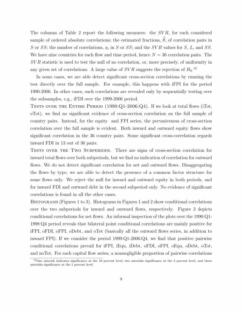
The columns of Table 2 report the following measures: the SV R, for each considered

sample of ordered absolute correlations; the estimated fractions, θ̂, of correlation pairs in

S or SS; the number of correlations, η, in S or SS; and the SV R values for S, L, and SS.

We have nine countries for each flow and time period, hence N = 36 correlation pairs. The

SV R statistic is used to test the null of no correlation, or, more precisely, of uniformity in

any given set of correlations. A large value of SV R suggests the rejection of H0.12

In some cases, we are able detect significant cross-section correlations by running the

test directly over the full sample. For example, this happens with iFPI for the period

1990-2006. In other cases, such correlations are revealed only by sequentially testing over

the subsamples, e.g., iFDI over the 1999-2006 period.

Tests over the Entire Period (1990:Q1-2006:Q4). If we look at total flows (iTot,

oTot), we find no significant evidence of cross-section correlation on the full sample of

country pairs. Instead, for the equity and FPI series, the pervasiveness of cross-section

correlation over the full sample is evident. Both inward and outward equity flows show

significant correlation in the 36 country pairs. Some significant cross-correlation regards

inward FDI in 13 out of 36 pairs.

Tests over the Two Subperiods. There are signs of cross-section correlation for

inward total flows over both subperiods, but we find no indication of correlation for outward

flows. We do not detect significant correlation for net and outward flows. Disaggregating

the flows by type, we are able to detect the presence of a common factor structure for

some flows only. We reject the null for inward and outward equity in both periods, and

for inward FDI and outward debt in the second subperiod only. No evidence of significant

correlations is found in all the other cases.

Histograms (Figures 1 to 3). Histograms in Figures 1 and 2 show conditional correlations

over the two subperiods for inward and outward flows, respectively. Figure 3 depicts

conditional correlations for net flows. An informal inspection of the plots over the 1990:Q1-

1998:Q4 period reveals that bilateral point conditional correlations are mainly positive for

iFPI, oFDI, oFPI, oDebt, and oTot (basically all the outward flows series, in addition to

inward FPI). If we consider the period 1999:Q1-2006:Q4, we find that positive pairwise

conditional correlations prevail for iFPI, iEqu, iDebt, oFDI, oFPI, oEqu, oDebt, oTot,

and noTot. For each capital flow series, a nonnegligible proportion of pairwise correlations

12One asterisk indicates significance at the 10 percent level, two asterisks significance at the 5 percent level, and threeasterisks significance at the 1 percent level.

9

change sign from one period to the other.

The potential existence of common factors driving capital flows at the EU level, which we

can detect with Ng’s statistical procedure, is due to the magnitude of absolute correlations

between the flows of pairs of countries. The larger these correlations, the more likely

the existence of such a common factor. The histograms indicate which pairs of countries

contribute (and how much) to the rejection of the null of no cross-section correlations in

the considered samples.

Ordered Absolute Correlations (Figures 4 and 5). Figures 4 and 5 provide a

graphical representation of the ordered absolute correlation pairs for EU countries and for

each capital flow. As in the previous analysis, the full sample (1990:Q1-2006:Q4) is split

into two disjoint subsamples. If the curve connecting absolute correlations lies above the

45-degree line passing through the origin of the axes, absolute correlations have increased

from the first to the second subsample. This indicates that also the likelihood that capital

flows are driven by a common factor at the EU level has increased. The larger the distance

from the 45-degree line, the greater the likelihood. Curves below the 45-degree line have

an opposite interpretation.

A graphical inspection of the plots shows that absolute correlations have likely increased

for oTot, noTot, oEqu, oFDI, oFPI, and probably for oFDI. In the other cases, absolute

correlations seem to be fairly stable over the subperiods. Of note, conclusions from this

informal investigation cannot be definite. Instead, they are more informative if combined

with the formal inference on the spacings described earlier. For instance, pointwise positive

changes in absolute correlations may still not be enough to justify the claim of emergence

of a common factor on statistical grounds.

Correlation Changes

We try to establish whether the introduction of the euro in 1999 has been accompanied by

correlation changes between types of capital flows within each country in the sample. We

report descriptive statistics and inference for the two subperiods in Tables 3 through 5.

Results basically show no systematic pattern. Previous empirical evidence suggests that

iFDI and iDebt are negatively correlated for emerging countries (Smith and Valderrama,

forthcoming), and that iFDI and iFPI are negatively correlated during times of crisis

(Acharya, Shin, and Yorulmazer, 2007). In our dataset, most couples of gross flows have

10

mixed correlation signs.

Inward Flows. Correlations range widely from approximately minus 0.2 to 0.2 for the

couple iFPI-iDebt to almost minus 0.4 to 0.4 for the couple iDebt-iEqu. Some of the

correlations experience wide swings between periods. Unlike the large variations, which

are more likely to be detected as significant by our bootstrap-based tests, small shifts are

more challenging. We are able to detect only eight significant changes out of 36 using the

test based on the iterated bootstrap, 13 using the noniterated version of it. As for the

correlations between the two types of equity flows, we have two negative shifts (Finland

and Italy) and two positive shifts (France and Germany). Significant changes between

iFDI and iDebt are both negative (Finland and the Netherlands), whereas they are mixed

in sign between iFPI and iDebt. The only cases of significant correlation changes between

iDebt and iEqu occur in Finland (down by 0.56) and Italy (down by 0.78), findings similar

to those in Smith and Valderrama (forthcoming) for emerging countries.

Outward Flows. Table 4 shows results for outward flows. The magnitudes and ranges

of correlations are generally similar to those observed for inward flows. Swings between

periods are somewhat smaller, except for the United Kingdom. A majority of countries

shows positive correlations between outward portfolio flows and oDebt. On the other hand,

outcomes for the other flows look mixed. Our test delivers significant changes only for a

handful of countries: twice when the iterated bootstrap is applied and four times (out of

36) when the noniterated bootstrap is run. We find a statistically significant decrease in

correlations between outward FDI and FPI only for Italy and Sweden, whereas correlation

shifts are significantly positive only for the United Kingdom (outward FDI and FPI, and

outward FPI and debt).

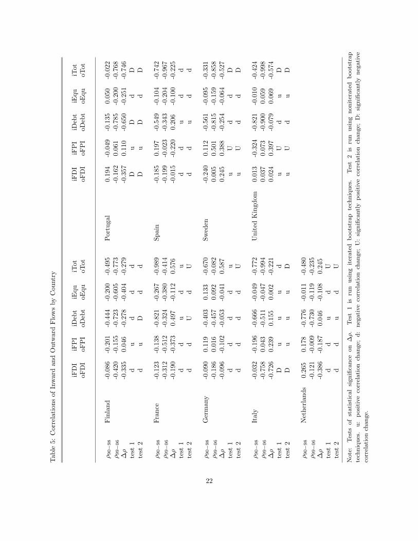
Inward and Outward Flows by Type of Flow and Country. In Table 5 we

report results coming from tests run between inward and outward series for each type of

flow. The range of correlations is definitely larger than in the two previous tables and a

ranking of the magnitude of correlations is clearer. Inward and outward debt flows are

almost always negatively correlated, with larger negative correlations reaching the value

of minus 0.9, as in the United Kingdom. Other flows are less correlated, with values

similar to those in the previous tables, and their signs are mixed. This finding may be

consistent with the fact that debt flows respond to interest rate differentials, whereas FDI

and FPI are less likely to react to changes in nominal returns. This result reinforces

11

our belief that looking at net flows might only lead to incorrect conclusions and that it is

ultimately worth looking at disaggregated flows. Correlations between inward and outward

total flows are positive and large, mostly dominated by the dynamics of debt flows. We

detect significantly negative changes between iFDI and oFDI (Italy and Portugal), and

iDebt and oDebt (Finland and Portugal). The signs of significant changes between total

flows are mixed, positive for France, Germany, and the Netherlands, negative for Italy,

Portugal, Sweden and the United Kingdom. Also note that, in a majority of instances,

point estimates of absolute correlations increase from one subperiod to the next.

5 Conclusions

In this paper we study the cross-section correlation of net, total, and disaggregated capital

flows for nine major source and recipient European Union countries. Our aim is to de-

termine whether it is reasonable to model the EU as an integrated economic entity when

observed as the source and destination of capital flows, for example as a counterpart of

the United States in two-country DSGE models with international portfolios. We first use

Ng (2006)’s uniform spacing method to establish the extent of cross-section correlations

and to determine which flows comove more. We find that a common factor structure is

suitable for equity flows and little evidence that a common factor drives the other flows,

except for inward total flows, inward FDI, and outward debt during the euro years. Hence

– as suggested by recent theoretical contributions – the analysis of countries’ gross assets

and liabilities and their disaggregation into different types might be useful, when capital

flows are interpreted as adjustments to country portfolios.

We also study whether the correlations between types of flows have changed since the

introduction of the euro. We find mixed evidence of significant changes, but we notice that,

in a majority of cases, point estimates of absolute correlations increase from one subperiod

to the next. This finding is consistent with the claim that EU capital flows are possibly

driven by a common factor.

12

References

Acharya, Viral V., Hyun Song Shin, and Tanj Yorulmazer (2007): “Fire-Sale FDI,” CEPR

Discussion Paper No. 6319.

Andrews, Donald W.K. (2005): “Cross-section Regression with Common Shocks,” Econo-

metrica, 73(5), 1551–1585.

Contessi, Silvio, Pierangelo De Pace, and Johanna Francis (2008): “The Cyclical Properties

of Disaggregated Capital Flows,” Federal Reserve Bank of St. Louis, manuscript.

De Pace, Pierangelo (2008): “Currency Union, Free-Trade Areas, and Business Cycle

Synchronization,” Johns Hopkins University, manuscript.

Devereux, Michael, and Alan Sutherland (2006): “Solving for Country Portfolios in Open

Economy Macro Models,” CEPR Discussion Paper No. 5966.

(forthcoming): “A Portfolio Model of Capital Flows to Emerging Markets,” Journal

of Development Economics.

DiCiccio, Thomas J., Michael A. Martin, and G. Alastair Young (1992): “Fast and Accu-

rate Approximate Double Boostrap Confidence Intervals,” Biometrika, 79(2), 285–295.

Doyle, Brian, and John Faust (2005): “Breaks in the Variability and Co-Movement of G-7

Economic Growth,” Review of Economics and Statistics, 87(4), 721–740.

Ekinci, Mehmet Fatih, Sebnem Kalemli-Ozcan, and Bent E. Sorensen (2008): “Integration

within EU Countries: The Role of Institutions, Confidence, and Trust,” in NBER Inter-

national Seminar on Macroeconomics 2007, ed. by F. G. Clarida, Richard. University of

Chicago Press.

Herrera, Ana Maria, Irina Murtazashvili, and Elena Pesavento (2008): “The Comovement

in Inventories and in sales: Higher and Higher,” Economics Letters, 99(1), 155–158.

13

IMF (2007): International Financial Statistics of the International Monetary Fund. Wash-

ington D.C.: International Monetary Fund.

Kaminsky, Graciela L., Carmen M. Reinhart, and Carlos A. Vegh (2004): “When it Rains,

it Pours: Procyclical Capital Flows and Macroeconomic Policies,” in NBER Macroe-

conomics Annual 2004, ed. by M. Gertler, and K. Rogoff. Cambridge, MA: The MIT

Press.

Kose, Ayhan M., Eswar S. Prasad, and Marco E. Terrones (forthcoming): “Does Financial

Globalization Promote Risk Sharing?,” Journal of Development Economics.

Lane, Philip, and Gian-Maria Milesi Ferretti (2007): “The External Wealth of Nations

Mark II: Revised and Extended Estimates of Foreign Assets and Liabilities,” Journal of

International Economics, 73(November), 223–250.

Levchenko, Andrei, and Paolo Mauro (2007): “Do Some Forms of Financial Flows Help

Protect from Sudden Stops?,” World Bank Economic Review, 21(3), 389–411.

Levy-Yeyati, Eduardo, Ugo Panizza, and Eduardo Ernesto Stein (2007): “The cyclical

nature of North-South FDI flows,” Journal of International Money and Finance, 26(1),

104–130.

Lipsey, Robert E. (1999): “The Role of FDI in International Capital Flows,” in Interna-

tional Capital Flows, ed. by M. Feldstein. Chicago: University of Chicago Press.

Neumann, Rebecca, Ron Penl, and Altin Tanku (2006): “Volatility of capital flows and

financial liberalization: Do specific flows respond differently?,” University of Wisconsin-

Milwakee Working Paper No. 06-202.

Ng, Serena (2006): “Testing Cross-Section Correlation in Panel Data Using Spacings,”

Journal of Business and Economic Statistics, 24(January), 12–23.

Rothenberg, Alexander, and Francis E. Warnock (2006): “Sudden Flight and True Sudden

Stops,” NBER Working Paper No. 12726.

14

Smith, Katherine, and Diego Valderrama (forthcoming): “The composition of capital flows

when emerging market firms face financing constraints,” Journal of Development Eco-

nomics.

Tille, Cedric, and Eric van Wincoop (2008): “International Capital Flows,” University of

Virginia, manuscript.

Appendix - Bootstrap Tests for Correlation Changes

Let ρ be the unconditional correlation coefficient between two time series, ρ1 the uncon-

ditional correlation over the first sample, and ρ2 the unconditional correlation over the

second sample. We are interested in testing whether the parameter shift, ∆ρ = (ρ2 − ρ1),

is statistically significant and formally consider the statistical test with size (1− α) ∈ (0, 1):

H0 : ∆ρ = (ρ2 − ρ1) = 0

H1 : ∆ρ = (ρ2 − ρ1) 6= 0.

Our inference is based on the construction of two-sided α-level confidence intervals

from the bootstrap distribution of ∆̂ρ.13 This allows us to test for significant breaks and

directly infer the direction of the shift. We apply bootstrap techniques to the data and

also use bootstrap iteration to estimate confidence intervals with potentially improved

accuracy. Namely, we derive iterated bootstrap percentile confidence intervals and iterated

bias-corrected (BC) percentile confidence intervals (as described in DiCiccio, Martin, and

Young, 1992). We interpret significant shifts at the 5 percent or 10 percent level as signs

of parameter instability over the sample.

Constructing Bootstrap Distributions

In the simple case of two capital flows series for two countries, A and B, let XA,t =

{XA,s}Ts=1 and XB,t = {XB,s}Ts=1 denote the two observed time series, with Br being

an exogenous breakpoint. Each series is split into two subsamples, X1A,t = {XA,s}Brs=1,

X1B,t = {XB,s}Brs=1, X2

A,t = {XA,s}Ts=Br+1, and X2B,t = {XB,s}Ts=Br+1. Let I1, I2, ... be a

13 We refer to two-sided equal-tailed confidence intervals. They are equal-tailed because they attempt to place equalprobability in each tail.

15

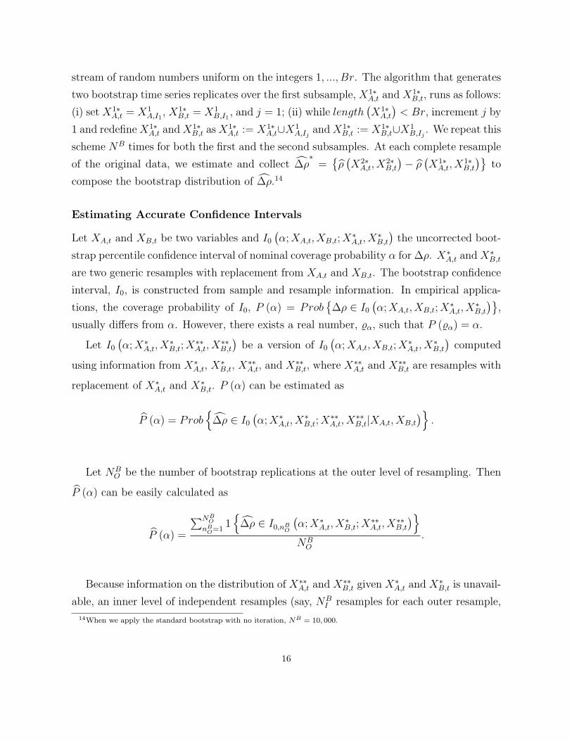
stream of random numbers uniform on the integers 1, ..., Br. The algorithm that generates

two bootstrap time series replicates over the first subsample, X1∗A,t and X1∗

B,t, runs as follows:

(i) set X1∗A,t = X1

A,I1, X1∗

B,t = X1B,I1

, and j = 1; (ii) while length(X1∗A,t

)< Br, increment j by

1 and redefineX1∗A,t andX1∗

B,t asX1∗A,t := X1∗

A,t∪X1A,Ij

andX1∗B,t := X1∗

B,t∪X1B,Ij

. We repeat this

scheme NB times for both the first and the second subsamples. At each complete resample

of the original data, we estimate and collect ∆̂ρ∗

={ρ̂(X2∗A,t, X

2∗B,t

)− ρ̂

(X1∗A,t, X

1∗B,t

)}to

compose the bootstrap distribution of ∆̂ρ.14

Estimating Accurate Confidence Intervals

Let XA,t and XB,t be two variables and I0

(α;XA,t, XB,t;X

∗A,t, X

∗B,t

)the uncorrected boot-

strap percentile confidence interval of nominal coverage probability α for ∆ρ. X∗A,t and X∗B,t

are two generic resamples with replacement from XA,t and XB,t. The bootstrap confidence

interval, I0, is constructed from sample and resample information. In empirical applica-

tions, the coverage probability of I0, P (α) = Prob{

∆ρ ∈ I0

(α;XA,t, XB,t;X

∗A,t, X

∗B,t

)},

usually differs from α. However, there exists a real number, %α, such that P (%α) = α.

Let I0

(α;X∗A,t, X

∗B,t;X

∗∗A,t, X

∗∗B,t

)be a version of I0

(α;XA,t, XB,t;X

∗A,t, X

∗B,t

)computed

using information from X∗A,t, X∗B,t, X

∗∗A,t, and X∗∗B,t, where X∗∗A,t and X∗∗B,t are resamples with

replacement of X∗A,t and X∗B,t. P (α) can be estimated as

P̂ (α) = Prob{

∆̂ρ ∈ I0

(α;X∗A,t, X

∗B,t;X

∗∗A,t, X

∗∗B,t|XA,t, XB,t

)}.

Let NBO be the number of bootstrap replications at the outer level of resampling. Then

P̂ (α) can be easily calculated as

P̂ (α) =

∑NBO

nBO=11{

∆̂ρ ∈ I0,nBO

(α;X∗A,t, X

∗B,t;X

∗∗A,t, X

∗∗B,t

)}NBO

.

Because information on the distribution of X∗∗A,t and X∗∗B,t given X∗A,t and X∗B,t is unavail-

able, an inner level of independent resamples (say, NBI resamples for each outer resample,

14When we apply the standard bootstrap with no iteration, NB = 10, 000.

16

nBO) from X∗A,t and X∗B,t is executed to outline the features of that distribution.15 The

bootstrap estimate for %α is the solution, %̂α, to the equation P̂ (%α) = α ∴ %̂α = P̂−1 (α).16

The iterated bootstrap confidence interval for ∆ρ is then I1

(%̂α;XA,t, XB,t;X

∗A,t, X

∗B,t

).

15We use 1, 000 replications for the outer bootstrap; 500 for the inner bootstrap. Note the presence of a serious trade-offbetween the number of resamples, which affects the overall accuracy of estimations, and computation time.

16With discrete bootstrap distributions, an exact solution for this equation cannot always be found, unless we use smoothing

techniques. We choose the smallest value %̂α such that P̂ (%̂α) is as close as possible to α, that is, such that∣∣∣P̂ (%α)− α

∣∣∣ is

minimized over a grid of values and additional conditions defining tolerance are satisfied. Refer to De Pace (2008) for furtherinformation on the algorithm and other estimation procedures adopted in this paper.

17

Table 1: Classification of Capital Flows

Type Component

Foreign Direct Investment FDI [iFDI, oFDI]}

Total Equity [iEqu, oEqu]Foreign Portfolio Investment Equity [iFPI, oFPI]Debt

}Total Debt [iDebt, oDebt]Other Investment Other Debt

Total Flows [iTot, oTot, noTot]

18

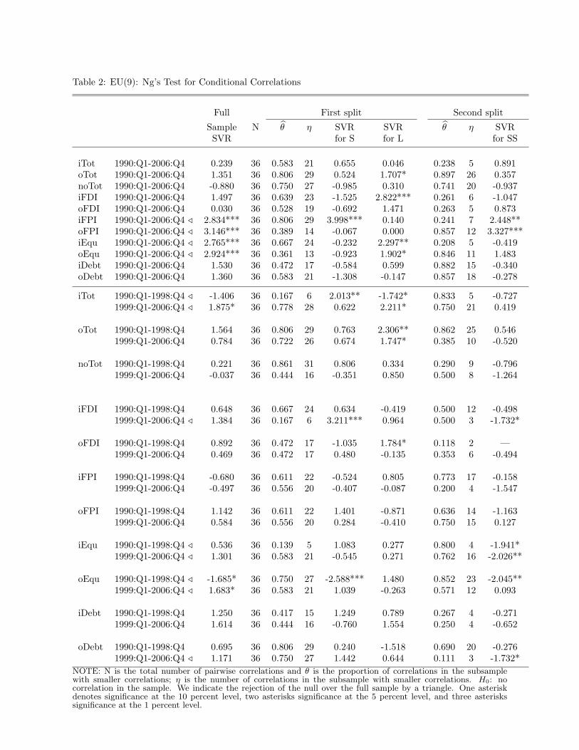
Table 2: EU(9): Ng’s Test for Conditional Correlations

Full First split Second split

Sample N θ̂ η SVR SVR θ̂ η SVRSVR for S for L for SS

iTot 1990:Q1-2006:Q4 0.239 36 0.583 21 0.655 0.046 0.238 5 0.891oTot 1990:Q1-2006:Q4 1.351 36 0.806 29 0.524 1.707* 0.897 26 0.357noTot 1990:Q1-2006:Q4 -0.880 36 0.750 27 -0.985 0.310 0.741 20 -0.937iFDI 1990:Q1-2006:Q4 1.497 36 0.639 23 -1.525 2.822*** 0.261 6 -1.047oFDI 1990:Q1-2006:Q4 0.030 36 0.528 19 -0.692 1.471 0.263 5 0.873iFPI 1990:Q1-2006:Q4 / 2.834*** 36 0.806 29 3.998*** 0.140 0.241 7 2.448**oFPI 1990:Q1-2006:Q4 / 3.146*** 36 0.389 14 -0.067 0.000 0.857 12 3.327***iEqu 1990:Q1-2006:Q4 / 2.765*** 36 0.667 24 -0.232 2.297** 0.208 5 -0.419oEqu 1990:Q1-2006:Q4 / 2.924*** 36 0.361 13 -0.923 1.902* 0.846 11 1.483iDebt 1990:Q1-2006:Q4 1.530 36 0.472 17 -0.584 0.599 0.882 15 -0.340oDebt 1990:Q1-2006:Q4 1.360 36 0.583 21 -1.308 -0.147 0.857 18 -0.278

iTot 1990:Q1-1998:Q4 / -1.406 36 0.167 6 2.013** -1.742* 0.833 5 -0.7271999:Q1-2006:Q4 / 1.875* 36 0.778 28 0.622 2.211* 0.750 21 0.419

oTot 1990:Q1-1998:Q4 1.564 36 0.806 29 0.763 2.306** 0.862 25 0.5461999:Q1-2006:Q4 0.784 36 0.722 26 0.674 1.747* 0.385 10 -0.520

noTot 1990:Q1-1998:Q4 0.221 36 0.861 31 0.806 0.334 0.290 9 -0.7961999:Q1-2006:Q4 -0.037 36 0.444 16 -0.351 0.850 0.500 8 -1.264

iFDI 1990:Q1-1998:Q4 0.648 36 0.667 24 0.634 -0.419 0.500 12 -0.4981999:Q1-2006:Q4 / 1.384 36 0.167 6 3.211*** 0.964 0.500 3 -1.732*

oFDI 1990:Q1-1998:Q4 0.892 36 0.472 17 -1.035 1.784* 0.118 2 —1999:Q1-2006:Q4 0.469 36 0.472 17 0.480 -0.135 0.353 6 -0.494

iFPI 1990:Q1-1998:Q4 -0.680 36 0.611 22 -0.524 0.805 0.773 17 -0.1581999:Q1-2006:Q4 -0.497 36 0.556 20 -0.407 -0.087 0.200 4 -1.547

oFPI 1990:Q1-1998:Q4 1.142 36 0.611 22 1.401 -0.871 0.636 14 -1.1631999:Q1-2006:Q4 0.584 36 0.556 20 0.284 -0.410 0.750 15 0.127

iEqu 1990:Q1-1998:Q4 / 0.536 36 0.139 5 1.083 0.277 0.800 4 -1.941*1999:Q1-2006:Q4 / 1.301 36 0.583 21 -0.545 0.271 0.762 16 -2.026**

oEqu 1990:Q1-1998:Q4 / -1.685* 36 0.750 27 -2.588*** 1.480 0.852 23 -2.045**1999:Q1-2006:Q4 / 1.683* 36 0.583 21 1.039 -0.263 0.571 12 0.093

iDebt 1990:Q1-1998:Q4 1.250 36 0.417 15 1.249 0.789 0.267 4 -0.2711999:Q1-2006:Q4 1.614 36 0.444 16 -0.760 1.554 0.250 4 -0.652

oDebt 1990:Q1-1998:Q4 0.695 36 0.806 29 0.240 -1.518 0.690 20 -0.2761999:Q1-2006:Q4 / 1.171 36 0.750 27 1.442 0.644 0.111 3 -1.732*

NOTE: N is the total number of pairwise correlations and θ is the proportion of correlations in the subsamplewith smaller correlations; η is the number of correlations in the subsample with smaller correlations. H0: nocorrelation in the sample. We indicate the rejection of the null over the full sample by a triangle. One asteriskdenotes significance at the 10 percent level, two asterisks significance at the 5 percent level, and three asteriskssignificance at the 1 percent level.

Tab

le3:

Cor

rela

tion

sof

Inw

ard

Flo

ws

byC

ount

ry

iFD

IiF

DI

iFP

IiD

ebt

iFD

IiF

DI

iFP

IiD

ebt

iFP

IiD

ebt

iDeb

tiE

quiF

PI

iDeb

tiD

ebt

iEqu

ρ90−

98

Fin

land

0.17

20.

333

0.05

40.

281

Por

tuga

l-0

.055

0.21

7-0

.011

-0.0

58ρ99−

06

-0.2

21-0

.274

-0.2

74-0

.274

-0.1

520.

153

-0.3

65-0

.134

∆ρ

-0.3

93-0

.607

-0.3

28-0

.556

-0.0

97-0

.064

-0.3

54-0

.075

test

1D

DD

Dd

dd

dte

st2

DD

DD

dd

Dd

ρ90−

98

Fran

ce-0

.085

0.08

4-0

.316

-0.2

11Sp

ain

0.02

3-0

.137

0.02

0-0

.024

ρ99−

06

0.23

40.

163

0.16

30.

169

-0.1

99-0

.049

0.13

1-0

.047

∆ρ

0.31

90.

080

0.47

90.

380

-0.2

220.

088

0.11

1-0

.023

test

1u

uU

ud

uu

dte

st2

Uu

Uu

du

ud

ρ90−

98

Ger

man

y-0

.269

-0.0

66-0

.212

-0.1

60Sw

eden

-0.0

990.

179

-0.1

72-0

.063

ρ99−

06

0.20

30.

084

0.05

3-0

.032

0.20

50.

173

-0.2

180.

140

∆ρ

0.47

20.

150

0.26

60.

127

0.30

5-0

.007

-0.0

460.

203

test

1u

uu

uu

dd

ute

st2

Uu

uu

ud

du

ρ90−

98

Ital

y0.

287

0.11

60.

455

0.39

8U

nite

dK

ingd

om-0

.042

-0.1

20-0

.175

-0.0

91ρ99−

06

-0.1

310.

346

-0.3

03-0

.380

-0.1

58-0

.160

0.19

20.

021

∆ρ

-0.4

180.

230

-0.7

58-0

.777

-0.1

16-0

.041

0.36

70.

112

test

1d

uD

Dd

du

ute

st2

Du

DD

dd

Uu

ρ90−

98

Net

herl

ands

-0.0

390.

102

0.03

3-0

.213

ρ99−

06

-0.1

40-0

.263

0.13

7-0

.108

∆ρ

-0.1

01-0

.365

0.10

40.

105

test

1d

Du

ute

st2

dD

uu

Note

:T

ests

of

stati

stic

al

signifi

cance

on

∆ρ.

Tes

t1

isru

nusi

ng

iter

ate

db

oots

trap

tech

niq

ues

.T

est

2is

run

usi

ng

nonit

erate

db

oots

trap

tech

niq

ues

.u:

posi

tive

corr

elati

on

change;

d:

neg

ati

ve

corr

elati

on

change;

U:

signifi

cantl

yp

osi

tive

corr

elati

on

change;

D:

signifi

cantl

yneg

ati

ve

corr

elati

on

change.

20

Tab

le4:

Cor

rela

tion

sof

Out

war

dF

low

sby

Cou

ntry

oFD

IoF

DI

oFP

IoD

ebt

oFD

IoF

DI

oFP

IoD

ebt

oFP

IoD

ebt

oDeb

toE

quoF

PI

oDeb

toD

ebt

oEqu

ρ90−

98

Fin

land

0.02

0-0

.358

0.12

0-0

.314

Por

tuga

l-0

.100

-0.2

330.

112

-0.1

05ρ99−

06

-0.1

74-0

.223

0.18

1-0

.160

-0.1

89-0

.012

0.16

70.

064

∆ρ

-0.1

940.

135

0.06

20.

154

-0.0

890.

221

0.05

50.

169

test

1d

uu

ud

uu

ute

st2

du

uu

du

uu

ρ90−

98

Fran

ce0.

016

-0.1

790.

114

-0.1

61Sp

ain

-0.1

82-0

.120

0.12

9-0

.177

ρ99−

06

0.12

0-0

.037

0.09

6-0

.032

-0.1

390.

009

0.10

60.

020

∆ρ

0.10

40.

142

-0.0

180.

128

0.04

20.

129

-0.0

220.

197

test

1u

ud

uu

ud

ute

st2

uu

du

uu

du

ρ90−

98

Ger

man

y0.

057

0.26

2-0

.233

-0.1

71Sw

eden

0.18

00.

155

0.01

50.

100

ρ99−

06

0.00

80.

243

-0.1

040.

291

-0.2

180.

196

0.18

70.

361

∆ρ

-0.0

48-0

.019

0.12

90.

462

-0.3

990.

040

0.17

20.

261

test

1d

du

uD

uu

ute

st2

dd

uu

Du

uu

ρ90−

98

Ital

y0.

154

0.02

3-0

.101

-0.0

04U

nite

dK

ingd

om-0

.041

-0.0

55-0

.340

-0.2

06ρ99−

06

-0.1

57-0

.137

0.18

80.

109

0.37

1-0

.102

0.05

20.

054

∆ρ

-0.3

11-0

.160

0.28

90.

113

0.41

2-0

.047

0.39

20.

260

test

1D

du

uu

du

ute

st2

Dd

uu

Ud

Uu

ρ90−

98

Net

herl

ands

-0.0

38-0

.152

-0.2

59-0

.302

ρ99−

06

-0.2

880.

085

-0.3

49-0

.369

∆ρ

-0.2

490.

237

-0.0

89-0

.068

test

1d

ud

dte

st2

du

dd

Note

:T

ests

of

stati

stic

al

signifi

cance

on

∆ρ.

Tes

t1

isru

nusi

ng

iter

ate

db

oots

trap

tech

niq

ues

.T

est

2is

run

usi

ng

nonit

erate

db

oots

trap

tech

niq

ues

.u:

posi

tive

corr

elati

on

change;

d:

neg

ati

ve

corr

elati

on

change;

U:

signifi

cantl

yp

osi

tive

corr

elati

on

change;

D:

signifi

cantl

yneg

ati

ve

corr

elati

on

change.

21

Tab

le5:

Cor

rela

tion

sof

Inw

ard

and

Out

war

dF

low

sby

Cou

ntry

iFD

IiF

PI

iDeb

tiE

quiT

otiF

DI

iFP

IiD

ebt

iEqu

iTot

oFD

IoF

PI

oDeb

toE

quoT

otoF

DI

oFP

IoD

ebt

oEqu

oTot

ρ90−

98

Fin

land

-0.0

86-0

.201

-0.4

44-0

.200

-0.4

95P

ortu

gal

0.19

4-0

.049

-0.1

350.

050

-0.0

22ρ99−

06

-0.4

20-0

.155

-0.7

23-0

.605

-0.7

73-0

.162

0.06

1-0

.785

-0.2

00-0

.768

∆ρ

-0.3

350.

046

-0.2

78-0

.404

-0.2

79-0

.357

0.11

0-0

.650

-0.2

51-0

.746

test

1d

ud

dd

Du

Dd

Dte

st2

du

Dd

dD

uD

dD

ρ90−

98

Fran

ce-0

.123

-0.1

38-0

.821

-0.2

67-0

.989

Spai

n-0

.185

0.19

7-0

.549

-0.1

04-0

.742

ρ99−

06

-0.3

12-0

.512

-0.3

24-0

.380

-0.4

14-0

.199

-0.0

23-0

.343

-0.2

04-0

.967

∆ρ

-0.1

90-0

.373

0.49

7-0

.112

0.57

6-0

.015

-0.2

200.

206

-0.1

00-0

.225

test

1d

du

du

dd

ud

dte

st2

dd

Ud

Ud

du

dd

ρ90−

98

Ger

man

y-0

.090

0.11

9-0

.403

0.13

3-0

.670

Swed

en-0

.240

0.11

2-0

.561

-0.0

95-0

.331

ρ99−

06

-0.1

860.

016

-0.4

570.

092

-0.0

820.

005

0.50

1-0

.815

-0.1

59-0

.858

∆ρ

-0.0

96-0

.102

-0.0

53-0

.041

0.58

70.

245

0.38

8-0

.254

-0.0

64-0

.527

test

1d

dd

du

uU

dd

Dte

st2

dd

dd

Uu

Ud

dD

ρ90−

98

Ital

y-0

.032

-0.1

96-0

.666

-0.0

49-0

.772

Uni

ted

Kin

gdom

0.01

3-0

.324

-0.8

21-0

.010

-0.4

24ρ99−

06

-0.7

580.

043

-0.5

11-0

.047

-0.9

940.

037

0.07

3-0

.900

0.05

9-0

.998

∆ρ

-0.7

260.

239

0.15

50.

002

-0.2

210.

024

0.39

7-0

.079

0.06

9-0

.574

test

1D

uu

ud

uU

du

Dte

st2

Du

uu

Du

Ud

uD

ρ90−

98

Net

herl

ands

0.26

50.

178

-0.7

76-0

.011

-0.4

80ρ99−

06

-0.1

21-0

.009

-0.7

30-0

.119

-0.2

35∆ρ

-0.3

86-0

.187

0.04

6-0

.108

0.24

5te

st1

dd

ud

Ute

st2

dd

ud

U

Note

:T

ests

of

stati

stic

al

signifi

cance

on

∆ρ.

Tes

t1

isru

nusi

ng

iter

ate

db

oots

trap

tech

niq

ues

.T

est

2is

run

usi

ng

nonit

erate

db

oots

trap

tech

niq

ues

.u:

posi

tive

corr

elati

on

change;

d:

neg

ati

ve

corr

elati

on

change;

U:

signifi

cantl

yp

osi

tive

corr

elati

on

change;

D:

signifi

cantl

yneg

ati

ve

corr

elati

on

change.

22

Figure 1: Conditional correlations by type of inward flow

iFDI

-0.4

-0.2

0

0.2

0.4

0.6

0.8

SPA

SW

E

FRA

GER

POR

SPA

FRA

SW

E

NE

T S

WE

FRA

UK

FRA

ITA

PO

R U

K

GE

R N

ET

FIN

SW

E

FIN

GER

SWE

UK

NET

U

K

FRA

NET

GER

ITA

FIN

SPA

GER

SPA

FIN

NE

T

FIN

FR

A

NE

T P

OR

FRA

SPA

ITA

UK

NET

SP

A

ITA

SW

E

POR

SW

E

FRA

PO

R

GER

PO

R

ITA

PO

R

FIN

ITA

SPA

UK

GE

R U

K

ITA

SPA

GER

SW

E

FIN

UK

FIN

PO

R

ITA

NE

T

iFPI

-0.4

-0.2

0

0.2

0.4

0.6

0.8

ITA

SPA

POR

SPA

POR

SW

E

ITA

SW

E

GER

SPA

FIN

NE

T

FIN

ITA

FRA

NET

SWE

UK

FRA

GER

FRA

PO

R

NET

SP

A

FIN

PO

R

GE

R N

ET

FIN

GER

FIN

UK

FRA

ITA

NE

T S

WE

SPA

UK

ITA

PO

R

GER

PO

R

ITA

NE

T

FRA

UK

FIN

SW

E

GER

SW

E

FRA

SW

E

NE

T U

K

NE

T P

OR

ITA

UK

SPA

SW

E

FRA

SPA

GE

R U

K

FIN

SPA

GER

ITA

FIN

FR

A

PO

R U

K

iEqu

-0.4

-0.2

0

0.2

0.4

0.6

0.8

POR

SPA

NET

SP

A

FIN

GER

GE

R U

K

FIN

NE

T

POR

SW

E

NE

T U

K

ITA

SPA

ITA

SW

E

GER

PO

R

PO

R U

K

SWE

UK

GER

ITA

FIN

PO

R

FRA

PO

R

SPA

UK

ITA

PO

R

FIN

ITA

GE

R N

ET

NE

T P

OR

FIN

SPA

FRA

UK

NE

T S

WE

FIN

FR

A

GER

SPA

FIN

SW

E

ITA

NE

T

FRA

ITA

FRA

GER

ITA

UK

FIN

UK

FRA

SW

E

FRA

NET

SPA

SW

E

FRA

SPA

GER

SW

E

iDebt

-0.4

-0.2

0

0.2

0.4

0.6

0.8

FRA

NET

NE

T U

K

FIN

UK

NE

T S

WE

FIN

SPA

GE

R N

ET

PO

R U

K

GER

SW

E

FIN

GER

FIN

FR

A

ITA

NE

T

FIN

ITA

ITA

SW

E

SWE

UK

POR

SPA

FRA

PO

R

FRA

ITA

GER

PO

R

NET

SP

A

ITA

UK

FIN

PO

R

FIN

SW

E

POR

SW

E

SPA

SW

E

FIN

NE

T

NE

T P

OR

GER

SPA

ITA

SPA

FRA

SW

E

FRA

GER

FRA

SPA

GE

R U

K

FRA

UK

ITA

PO

R

GER

ITA

SPA

UK

Note: 1990:Q1-1998:Q4 (open bars) and 1999:Q1-2006:Q4 (solid bars)

23

Figure 2: Conditional correlations by type of outward flow

oFDI

-0.4

-0.2

0

0.2

0.4

0.6

0.8

GE

R N

ET

SPA

UK

POR

SPA

FRA

NET

FIN

PO

R

SPA

SW

E

FIN

SW

E

ITA

UK

GE

R U

K

FRA

SW

E

NE

T S

PA

FRA

ITA

SWE

UK

GER

ITA

GER

SPA

FRA

GER

NE

T S

WE

FRA

SPA

FRA

PO

R

FIN

SPA

ITA

SW

E

FIN

FR

A

FRA

UK

FIN

NE

T

PO

R U

K

FIN

GER

NE

T P

OR

GER

PO

R

FIN

ITA

GER

SW

E

ITA

SPA

ITA

NE

T

ITA

PO

R

NET

U

K

POR

SW

E

FIN

UK

oFPI

-0.4

-0.2

0

0.2

0.4

0.6

0.8

FIN

NE

T

ITA

NE

T

GE

R N

ET

NE

T P

OR

FRA

NET

SPA

UK

NE

T U

K

GER

ITA

GER

SW

E

FIN

SW

E

GER

SPA

ITA

PO

R

POR

SW

E

POR

SPA

GE

R U

K

FIN

SPA

NET

SP

A

FRA

SW

E

FRA

ITA

GER

PO

R

SPA

SW

E

FRA

GER

ITA

SW

E

NE

T S

WE

FRA

SPA

FIN

GER

FIN

FR

A

ITA

SPA

FRA

PO

R

ITA

UK

FRA

UK

PO

R U

K

SWE

UK

FIN

ITA

FIN

UK

FIN

PO

R

oEqu

-0.4

-0.2

0

0.2

0.4

0.6

0.8

FRA

NET

FIN

GER

POR

SPA

NET

SP

A

FRA

ITA

GER

SPA

ITA

PO

R

FRA

GER

PO

R U

K

SPA

SW

E

GER

ITA

SPA

UK

FIN

PO

R

FRA

SW

E

GE

R U

K

NE

T P

OR

FIN

SW

E

POR

SW

E

FIN

NE

T

FIN

FR

A

GER

SW

E

GE

R N

ET

FRA

UK

GER

PO

R

SWE

UK

FRA

PO

R

ITA

SW

E

FIN

SPA

oDebt

-0.4

-0.2

0

0.2

0.4

0.6

0.8

FRA

NET

NE

T S

WE

NE

T P

OR

NE

T U

K

GER

ITA

FIN

ITA

ITA

SW

E

FIN

GER

FIN

FR

A

POR

SPA

POR

SW

E

FIN

PO

R

ITA

NE

T

FRA

ITA

NET

SP

A

FIN

SPA

GE

R N

ET

ITA

PO

R

PO

R U

K

FIN

SW

E

FRA

PO

R

GER

PO

R

GER

SW

E

FRA

GER

SPA

SW

E

ITA

SPA

SWE

UK

FIN

UK

ITA

UK

FIN

NE

T

GE

R U

K

GER

SPA

FRA

SPA

FRA

SW

E

SPA

UK

FRA

UK

Note: 1990:Q1-1998:Q4 (open bars) and 1999:Q1-2006:Q4 (solid bars)

24

Figure 3: Conditional correlations of net total outward flows

iTot

-0.4

-0.2

0

0.2

0.4

0.6

0.8

FRA

NET

NE

T S

WE

FIN

UK

GER

PO

R

PO

R U

K

FIN

SPA

FIN

FR

A

FIN

GER

SWE

UK

GE

R N

ET

FIN

ITA

ITA

NE

T

GER

SW

E

POR

SPA

NE

T U

K

FIN

NE

T

FRA

PO

R

ITA

UK

SPA

SW

E

FIN

PO

R

POR

SW

E

FRA

UK

FRA

SW

E

ITA

SW

E

NE

T P

OR

FRA

SPA

FRA

GER

FIN

SW

E

FRA

ITA

NET

SP

A

ITA

SPA

ITA

PO

R

GER

SPA

GER

ITA

GE

R U

K

SPA

UK

oTot

-0.4

-0.2

0

0.2

0.4

0.6

0.8

FRA

NET

NE

T S

WE

FIN

ITA

ITA

NE

T

SWE

UK

FRA

PO

R

PO

R U

K

GER

PO

R

FIN

SPA

GER

ITA

GER

SW

E

NET

SP

A

FIN

SW

E

ITA

SW

E

POR

SW

E

GE

R N

ET

ITA

PO

R

ITA

UK

SPA

SW

E

NE

T U

K

FRA

ITA

FIN

FR

A

FIN

PO

R

POR

SPA

NE

T P

OR

FRA

SW

E

ITA

SPA

FRA

SPA

FIN

GER

FRA

GER

FIN

UK

SPA

UK

FIN

NE

T

GER

SPA

FRA

UK

GE

R U

K

noTot

-0.4

-0.2

0

0.2

0.4

0.6

0.8

FIN

ITA

PO

R U

K

FIN

FR

A

FRA

GER

ITA

UK

FRA

PO

R

GER

SPA

ITA

NE

T

FRA

SW

E

POR

SW

E

ITA

SW

E

SPA

SW

E

GE

R U

K

GER

ITA

SWE

UK

FRA

UK

NE

T P

OR

GE

R N

ET

NE

T S

WE

FIN

NE

T

FRA

SPA

FIN

UK

FRA

ITA

GER

SW

E

NET

SP

A

ITA

PO

R

ITA

SPA

SPA

UK

FIN

PO

R

FIN

SPA

FRA

NET

NE

T U

K

FIN

GER

FIN

SW

E

GER

PO

R

POR

SPA

Note: 1990:Q1-1998:Q4 (open bars) and 1999:Q1-2006:Q4 (solid bars)

25

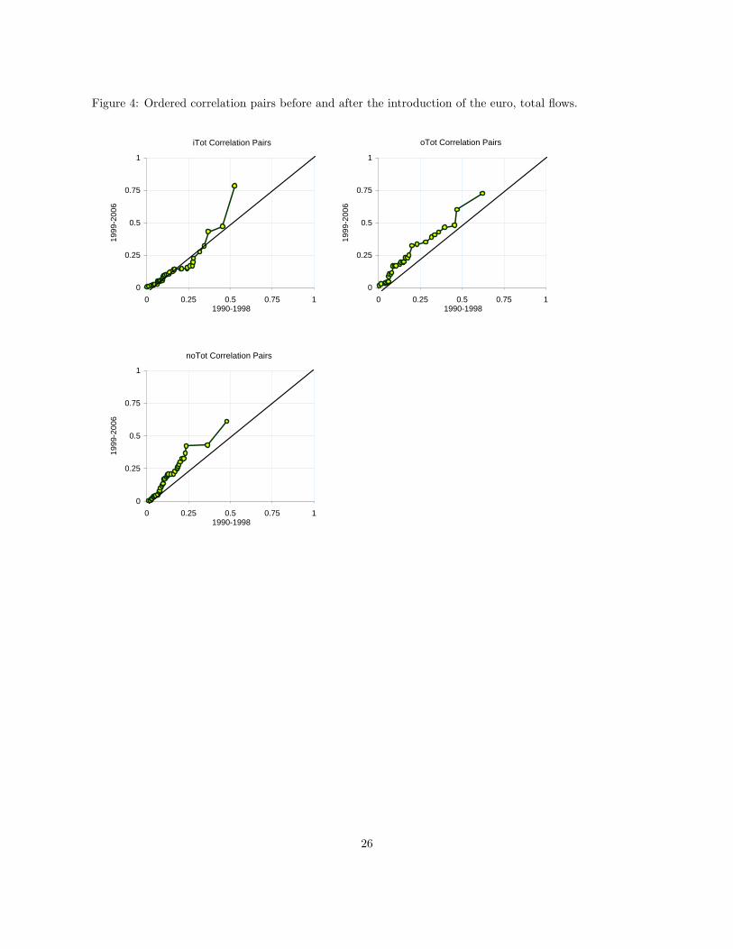
Figure 4: Ordered correlation pairs before and after the introduction of the euro, total flows.

iTot Correlation Pairs

0

0.25

0.5

0.75

1

0 0.25 0.5 0.75 11990-1998

1999

-200

6

oTot Correlation Pairs

0

0.25

0.5

0.75

1

0 0.25 0.5 0.75 11990-1998

1999

-200

6noTot Correlation Pairs

0

0.25

0.5

0.75

1

0 0.25 0.5 0.75 11990-1998

1999

-200

6

26

Figure 5: Ordered correlation pairs before and after the introduction of the euro, disaggregated flows.

iFDI Correlation Pairs

0

0.25

0.5

0.75

1

0 0.25 0.5 0.75 11990-1998

1999

-200

6

iFPI Correlation Pairs

0

0.25

0.5

0.75

1

0 0.25 0.5 0.75 11990-1998

1999

-200

6

oFDI Correlation Pairs

0

0.25

0.5

0.75

1

0 0.25 0.5 0.75 11990-1998

1999

-200

6

iEqu Correlation Pairs

0

0.25

0.5

0.75

1

0 0.25 0.5 0.75 11990-1998

1999

-200

6

oFPI Correlation Pairs

0

0.25

0.5

0.75

1

0 0.25 0.5 0.75 11990-1998

1999

-200

6

oEqu Correlation Pairs

0

0.25

0.5

0.75

1

0 0.25 0.5 0.75 11990-1998

1999

-200

6

iDebt Correlation Pairs

0

0.25

0.5

0.75

1

0 0.25 0.5 0.75 11990-1998

1999

-200

6

oDebt Correlation Pairs

0

0.25

0.5

0.75

1

0 0.25 0.5 0.75 11990-1998

1999

-200

6

27