auditing crypto currency transactions: anomaly …trap.ncirl.ie/3489/1/parismoore.pdf0 auditing...
TRANSCRIPT

0
Auditing Crypto Currency Transactions:
Anomaly Detection in Bitcoin
A report submitted in partial fulfilment of the requirements for the award of
the degree of
B.Sc (hons)
in
Computing (Data Analytics)
By
Paris Moore (X14485758)
Paris Moore | BSc Computing | May 13th, 2018

1
Declaration Cover Sheet for Project Submission
SECTION 2 Confirmation of Authorship
The acceptance of your work is subject to your signature on the following declaration:
I confirm that I have read the College statement on plagiarism (summarised overleaf and printed in
full in the Student Handbook) and that the work I have submitted for assessment is entirely my own
work.
Signature: __________________________
Date: ______________________________
Name: Paris Moore
Student ID: x14485758
Supervisor: Simon Caton

- 2 -
ABSTRACT
Both “big data” and “analytics” have become popular keywords in many
organizations. The power data analytics has on harnessing the increasing volumes, velocity and
complexity of data in a world of constant change and disruptive technologies has been recognized.
Many companies are making significant investments to better understand the impact of these
capabilities on their businesses. One area with significant potential is the transformation of the
audit. This project explores ways in which analytics can change and shape the work of accountants.
Anomaly detection plays a pivotal role in data mining since most outlying points contain
crucial information for further investigation. In the financial world which the Bitcoin network is a
part of, anomaly detection can indicate fraud. Using data mining tools such as Regression, we
simultaneously examine the relationship among variables whilst visually inspecting the data for
possible outliers. By doing so, I have chosen the world’s leading cryptocurrency, Bitcoin. This
project will conclude with an in-depth analysis on whether or not data analytics can shape how
effectively, and secure accountants can audit transactions by implementing analytics tools into their
daily protocols.
Keywords: Anomaly Detection, Bitcoin, Transactions, Regression, Accountancy, Analytics

- 3 -
Declaration Cover Sheet for Project Submission .............................................................................1
ABSTRACT .......................................................................................................................................2
INTRODUCTION ..............................................................................................................................5
MOTIVATION FOR THIS PROJECT ...........................................................................................6
DOMAIN CHALLENGES ..............................................................................................................6
BACKGROUND ............................................................................................................................7
RELATED WORK .............................................................................................................................7
Anomaly Detection ...................................................................................................................7
Clustering .................................................................................................................................8
Regression ...............................................................................................................................9
Unsupervised and Supervised Anomaly Detection .................................................................9
PROJECT AIM ............................................................................................................................... 10
TECHNOLOGIES USED ............................................................................................................... 10
R: 10
RStudio: 10
Tableau: 11
Microsoft Excel: ..................................................................................................................... 11
ALTERNATIVE TECHNOLOGIES EXPLORED ....................................................................... 11
Google BigQuery: ................................................................................................................. 11
Python: 11
Hadoop: 11
METHODOLOGY .......................................................................................................................... 12
Selection 13
13
Pre-processing ...................................................................................................................... 14
Transformation ...................................................................................................................... 14
Data Mining ........................................................................................................................... 14
Interpretation/Evaluation ....................................................................................................... 15
ANALYSIS & DESIGN ................................................................................................................... 16
USE CASES .............................................................................................................................. 16
DATA REQUIREMENTS ........................................................................................................... 16
IMPLEMENTATION ....................................................................................................................... 19
SET UP THE ENVIRONMENT ............................................................................................. 19
19
CLEANING THE DATA ......................................................................................................... 19
SAMPLING THE DATA ......................................................................................................... 20
DIMENSION REDUCTION ................................................................................................... 21

- 4 -
COMBINING THE DATA & BUILDING A DATA FRAME ..................................................... 22
22
ANALYZING AND EXPLORING THE DATA ........................................................................ 23
VISUALIZING THE DATA ..................................................................................................... 25
BUILDING THE MODELS..................................................................................................... 26
TESTING ....................................................................................................................................... 38
Unit testing: ........................................................................................................................... 38
CONCLUSION & FURTHER WORK ............................................................................................. 39
Final Thoughts ............................................................................................................................... 40
APPENDIX ..................................................................................................................................... 41
SUPERVISOR INTERACTION ................................................................................................. 41
PROJECT PROPOSAL ............................................................................................................. 43
Objectives ............................................................................................................................. 43
Motivation .............................................................................................................................. 44
Technical Approach .............................................................................................................. 44
Special resources required ................................................................................................... 44
Project Plan ............................................................................................................................... 45
PROJECT RESTRICTIONS ...................................................................................................... 47
Data 47
Time: 47
Cost: 47
Software: ............................................................................................................................... 47
Legal: 47
FUNCTIONAL/NON-FUNCTIONAL REQUIREMENTS ............................................................ 47
SECURITY REQUIREMENTS .............................................................................................. 47
AVAILABILITY REQUIREMENT ........................................................................................... 48
INTEGRITY REQUIREMENT ............................................................................................... 48
USER REQUIREMENTS ...................................................................................................... 48
TECHNICAL REPORT USE CASES ............................................................................................. 48
Requirement 1 <Gather Data> ............................................................................................. 48
Requirement 2 <Pre-processing> ......................................................................................... 49
Requirement 3:<Data Storage> ............................................................................................ 50
Requirement 4: <Analyse Data> ........................................................................................... 51
Requirement 5: <Machine Learning> ................................................................................... 52
Market Price vs All Variables ................................................................................................ 53
BIBLIOGRAPHY ............................................................................................................................ 55

5
INTRODUCTION
“It’s a massive leap to go from traditional audit approaches to one that fully integrates big data
and analytics in a seamless manner.”
– EY, How big data and analytics are transforming the audit.
Finance leaders are finding it very difficult to find accounting and financial professionals who
possess the technical skills to implement data analytic initiatives. In a recent survey by Robert Half,
Building a Team to Capitalize on the Promise of Big Data, 87 % of managers seek business
analytics skills in financial analysis. These significant figures are having an impact on the future
careers for accountants and whether or not there will still be a need for people with accountancy
and financial skills over a person with data analytic skills.
One of the primary tasks as an accountant is auditing. For this investigation, we will use the world’s
leading crypto currency, Bitcoin, to audit transactions. Bitcoin is a special type of transaction
system. It is traded on over 40 exchanges worldwide accepting over 30 different currencies and has
a current market capitalization of 9 billion dollars. Interest in Bitcoin has grown significantly with
over 250,000 transactions now taking place per day. It is on a sharing network known as the
blockchain that has publicly produced a ledger that contains every transaction ever processed. The
authenticity of each transaction is protected by digital signatures corresponding to the sending
addresses, allowing all users to have full control over sending bitcoins from their own Bitcoin
addresses.
With respect to transactional networks, comes those transactions who appear abnormally. We refer
to those as anomalies or outliers. In terms of financial transactions, we can assume they may be
fraudulent, or in fact may not be. A key goal would be to detect these anomalies to prevent future
illegal actions. It can also allow for some interesting findings about our data. Big data are huge sets
of information gathered that are so voluminous and complex that the average processing application
are inadequate to deal with them. This is where the need for some personnel with analytical or
technical experience is needed in order to optimize the data to gain as much knowledge as possible.
Big data challenges include capturing data, data storage, data analysis, search, sharing and transfer,
visualization, querying, updating and information privacy. If the work of an accountant can be
complete through these tasks, allowing for much more useless precise information, then will there
eventually be a need for accountants over someone with analytical ability? This research project
will investigate this using a large chunk of data from the bitcoin ledger.

- 6 -
MOTIVATION FOR THIS PROJECT
The underlying motivation for this project is the usefulness of analytic tools to audit a transactional
dataset. Ultimately the initial goal is the same as that for an accountant when it comes them auditing
a transactional ledger. But by applying highly technical algorithms, we hope for a more flawless
process with an in-depth analysis report answering beyond our initial question. Allowing for a
conclusion on accountancy versus analytics. To achieve this, we must clean, explore and optimise
our data in a way in which an accountancy cannot do so manually. Whether this be down to lack of
technical skill, resources or knowledge. By doing so, we can gain much more knowledge about our
data and gain a competitive advantage. To condense this research, the aim is to produce a fully
functional data mining model to represent our findings. Two areas’ well researched and explored
as an accountant, Outlier detection and Forecasting. Clustering and Regression are two models of
motivation for this project.
“The primary task of accountants, which extends to all the others, is to prepare and examine
financial records. They make sure that records are accurate and that taxes are paid properly and
on time. Accountants and auditors perform overviews of the financial operations of a business in
order to help it run efficiently.”
- https://www.allbusinessschools.com/accounting/job-description/
DOMAIN CHALLENGES
The challenges of this project are as follows:
1. Collecting of data will be challenging. Although, Bitcoin ledger can be openly sourced
online. The language of preference for this analysis was R. RStudio does not support
libraries in which you can pull straight from the bitcoin ledger, so my data will have to be
manually downloaded.
2. Choosing the right dataset in terms of size and complexity will be a big challenge for this
project. To optimize this projects potential, the data we acquire must be of high
dimensions.
3. Transforming the data to a manageable format will save future time spent loading data.
Data for projects such as these, spend the entirety of the time cleaning and formatting.
4. With big data, involves high computational requirements. A challenge for all industries
handling big data. The data must be reduced in size or else it will be unworkable even
with modern computers.
5. An existing knowledge of the data to be able to filter out the bulk of the noise is crucial.
The pre-processing stage will have a significant effect on the end results.
6. Defining what is an outlier will involve high technical ability. Targeting the features for
my model.
7. Sampling and dimension reduction is an extremely complicated topic. When is too much
and when is not enough? The risk of overfitting and underfitting can arise.
8. How the results are presented will play an important role in the interpretation of this
project. Ensuring the initial idea is constantly being re-visited and evaluated.
- 7 -
BACKGROUND
Accountancy was my main area of interest when I began researching courses and colleges. As I
began researching in further depth about the economy and degrees that would be “future proof”, I
came across a noticeable demand for students with computing degrees which left me where I am
today. The need for I.T experts has and still is a huge concern for many businesses. One area that
consistently stands out is, the concept of handling Big data and the different techniques and
methodologies to do so. Data Analytics is shaping businesses, especially in the financial sector
which has left a huge strain on accountancy jobs and the need for accountants over a data analyst.
This immediately caught my eye and I knew I wanted to research this further.
The first issue I ran into was what dataset could I analyse to explore this idea? It had to be relevant
and one that corresponds to data an accountant would work with. Knowing this dataset would
shape my project and the outcome I had to think long about it. At the project pitch, the dragons
suggested using a bitcoin dataset. Bitcoin is the world’s leading crypto currency. Due to the open
nature of Bitcoin it also poses another paradigm as opposed to traditional financial markets. It
operates on a decentralized, peer-to-peer and trustless system in which all transactions are posted
to an open ledger. This type of transparency is unheard of in other financial markets. I knew this
would add to my project and enable me to explore the world of crypto currency and blockchain
which has caught the eye of many huge companies recently.
RELATED WORK
There are many research projects and journals on Bitcoin as a crypto currency. Exploring any area
of the blockchain in general, is well researched and documented. However, with that in mind, my
aim is to compare my analysis on a transactional ledger using data and web mining algorithms and
techniques to highlight and showcase the power of analytics from an accountancy perspective. This
has not been done. To assist with this research, I have gained a lot of knowledge about anomaly
detection through related work, which is a huge motivation for this project. Some findings from
related work are documented as follows:
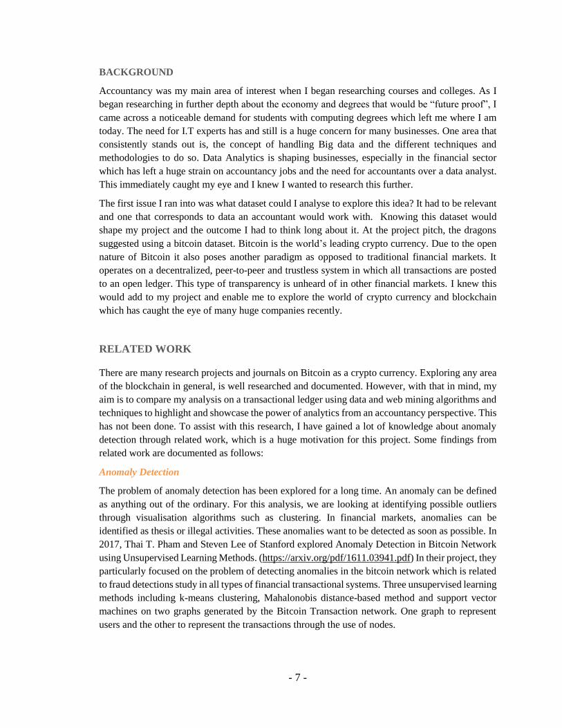
Anomaly Detection
The problem of anomaly detection has been explored for a long time. An anomaly can be defined
as anything out of the ordinary. For this analysis, we are looking at identifying possible outliers
through visualisation algorithms such as clustering. In financial markets, anomalies can be
identified as thesis or illegal activities. These anomalies want to be detected as soon as possible. In
2017, Thai T. Pham and Steven Lee of Stanford explored Anomaly Detection in Bitcoin Network
using Unsupervised Learning Methods. (https://arxiv.org/pdf/1611.03941.pdf) In their project, they
particularly focused on the problem of detecting anomalies in the bitcoin network which is related
to fraud detections study in all types of financial transactional systems. Three unsupervised learning
methods including k-means clustering, Mahalonobis distance-based method and support vector
machines on two graphs generated by the Bitcoin Transaction network. One graph to represent
users and the other to represent the transactions through the use of nodes.

- 8 -
Using the following features, In-degree, Out-degree, unique in-degree, unique out-degree,
clustering coefficient, average in and our transactions, average time, balance, creation date and
active duration, each feature is plotted on the transactional and user graphs. The features mean
different things for the two representations. The SVM method took a long time to run so therefore
data points were limited to 100,000. This method detected one known loss. The k-Means cluster,
which k=7 for both graphs, calculated the average of the ratios of detected anomaly distances to the
centroids over max distances. Only the top 100 outliers were targeted. The Mahalanobis Distance
based method detected one known theft. This studied concluded that only two known cases of theft
and loss out of 30 known cases were detected from the three documented unsupervised techniques,
resulting in the methods being unsuccessful in their entirety.
Clustering
Many metrics follow regular patterns correlated to determine normality. When that pattern becomes
skewed or scattered, it can cause some alarms to go off. For example, when the metric is correlated
to time, the key is to find its seasonality. Any activity outside of this “season” can be detected as
anomalous and thus resulting in the identification of fraud, theft etc. or some other interesting
discovery. K-means is one the most well-known and used algorithms for clustering. Clustering
classifies your data based on similar features within a particular cluster. All points within a cluster
have been identified by the algorithm as being similar among themselves and dissimilar to the data
of the other clusters.
Varun Chandola, Arindam Banerjee and Vipin Kumar -Anomaly Detection: A Survey, from the
University of Minnesota, evaluate clustering as an anomaly detection technique.
(https://dl.acm.org/citation.cfm?id=1541882). According to the authors, clustering-based anomaly
detection can be grouped into three categories:
1. Category one assumes that normal data instances belong to clusters while those
anomalous does not belong to any cluster. DBSXAN, ROCK and SNN
clustering are examples of category one.
2. Category two assumes normal data instances lie close to their closed cluster
centroid whilst those anomalous lies far aware from their closest cluster
centroid. K-means is an example of this.
3. Category three’s assumption is that normal data instances belong to large, dense
clusters, whist’s those anomalous either belong to small, sparse clusters.
Therefore, data belonging to clusters below are pre-declared threshold will be
identified as outliers. An example of this category is CBLOF clustering
approach where a local outlier factor is applied.
The survey concludes the section on clustering-based anomaly detection with an analysis on the
advantages and disadvantages of the technique. Some advantages are speedy test phase, operational
in an unsupervised mode and the complexity of the technique is small allowing it to adapt to other
more complex data types. Disadvantages include the dependency of the algorithm on performance
is based on the effectiveness of the clustering algorithm in capturing cluster structure of normal
instances. Also, several clustering algorithms force every instance to be assigned to a cluster which
may result in bypassing potential anomalies. Also, a good clustering-based anomaly detector is
extremely computationally complex and difficult to implement on large data.
- 9 -
Regression
Xiufeng Liu and Per Sieverts Nielsen from the University of Denmark explore Regression based
online Anomaly Detection for Smart Grid Data (file:///C:/Users/paris/Downloads/Regression-
based_Online_Anomaly_Detection_for_Smar.pdf). In this survey, they are using a data analytics
solution to an everyday problem, detection of unusual consumption behaviours of customers with
the widely used smart energy meters. Proposed in a supervised learning and statistical-based
approach, Regression. Effective use of regression as an anomalous detector would result in real-
time in order to minimise the compromised to the use of the energy, according to Xiufeng and Per.
“The efficiency of updating the detection model and the accuracy of the detection are the
important consideration for constructing such a real-time anomaly detection system. In this
paper, we propose a statistical anomaly detection method based on the consumption patterns of
smart grid data”
The model is composed of a short-term prediction algorithm, periodic auto regression and
Gaussian statistical distribution. This proposal was implemented and tested onto real-world data
and the results have validated the effectiveness and the efficiency of the proposed system with the
lambda architecture. The flexibility of regression was truly highlighted in this paper and used in a
way I had no seen or heard of before. This caught my attention and made me want to experiment
with it on a transaction dataset to see its limits. Ideally, we hope to detect anomalous behaviour
with this model, whilst still fulfilling its general usability, forecasting.
Unsupervised and Supervised Anomaly Detection
Supervised anomaly detection techniques require a dataset that has labeled instances for “normal”
and “abnormal” as well as a trained classifier. A typical approach would be to build a predictive
model for normal vs. anomaly classes. Any unseen data instance is compared against the model to
determine which class it belongs to. With supervised detection methods, we provide
examples(labels) and train a model to “recognize” and differentiate between different labels. We are
interested in predictions, i.e. using our feature vector X to predict or categorize label Y, or forecast
our numeric dependent variable Y. One approach uses graphs for modelling the normal data and
detect the irregularities in the graph for anomalies (Noble & Cook 2003). Another approach uses the
normal data to generate abnormal data and uses it as input for a classification algorithm (Gonzalez
& Dasgupta 2003).
Unsupervised anomaly detection techniques are more widely applicable because it does not make
any assumption about the availability of labeled training data. Instead, the techniques make other
assumptions about the data e.g. several techniques make the basic assumption that normal instances
are far more frequent than outliers. This frequently results in occurring patterns appearing normal,
whilst rare occurring patterns is typically considered as outliers. The unsupervised techniques
typically suffer from higher false alarm rate, because often times the underlying assumptions do not
hold true.

- 10 -
PROJECT AIM
Data analytics can certainly play a key role in many aspects of accounting. I will explore these
roles and apply analytic tools and techniques to transform dated auditing concepts into a
digitalized approach. Some of the key areas to concentrate on:
Aim 1: Boost competitiveness: Exploring ways to boost a company’s competitiveness through
the use of Predictive analytics techniques. This would allow accounting professionals to make
more accurate forecasts.
Aim 2: Manage Risks: This is a huge concern for businesses and the role of managing risks for
accountants have evolved from being solely based on compliance and internal controls to
assessing risks arising from a diverse range of areas. Techniques such as continuous auditing and
monitoring is proving to not be enough to monitor huge amounts of data.
Aim 3: Identify Fraud: Data analytics techniques are well-suited for detecting fraud and this is
an area I would like to highlight during this project. Similar, to managing risks, I will apply
analytics outlier detection methods to my dataset to identify anomalies in my dataset. Emerging
technologies in this area can allow a forensic accountant to quickly and effectively sieve through
large volumes of transactions to identify anomalies in data which can often be indicative of
fraudulent activity.
Aim 4: Explore Crypto currency and Blockchain: Another aim for this project, is to become
more knowledgeable and aware of the evolving world of blockchain. For this reason, I have
chosen the world’s leading crypto-currency, bitcoin, as my dataset.
Aim 5: Enhance Technical Skill and Knowledge: If successful, I hope this research can allow
for enhancement on not only my own technical ability, but for someone reading this and eager to
apply my knowledge to their problem successfully. Additionally, a student potentially
considering commencing a four-year course in accountancy becoming more leaning towards a
career in IT would be a huge success for me.
TECHNOLOGIES USED
R:
R is a programming language and environment for statistical computing and graphics. It is a GNU
project with similarity to the S languages. R is widely used for statistical and graphical techniques
such as time-series analysis, classification, regression and clustering. It is high extensible and
available as open-source online. I will use R to conduct in depth analysis on my data. It will be the
main language of choice for this project due to its wide variety of libraries and low limitations.
RStudio:
RStudio is an Integrated development environment (IDE) for R programming language. I will use
R in RStudio to create scripts to analyse the data sets. The R environment is successful in data
handling and storage facility, applying calculations from basic mean methods to extensive for loop
algorithms. It also graphically facilitates for data analysis. R is very extendable due to the vast
number of libraries available, many of which I have optimized in this project.

- 11 -
Tableau:
Tableau is a data visualization software application that allows the user to represent their findings
in a clear and concise way. Once I have completed the analysis of my data sets in RStudio using R
programming language I will use Tableau to represent my findings. Tableau uses the k-means
algorithm for clustering. This will allow my audience to have a greater understanding of this project
and my findings, both from technical and non-technical backgrounds. All graphs will be visible
from my dashboard, which I have created in tableau.
Microsoft Excel:
Microsoft Excel is a spreadsheet program that extends from the Microsoft Office Suite of
applications. It is a spreadsheet which represents tables of data arranged in rows and columns. Many
statistical analyses can be conducted in excel. This program in particular would be often used by
accountants for analysis. However, it would be about the limit in which they go technically. I used
to excel to read one of my datasets. I also transformed my .txt datasets into .csv files through the
use of R, as excel is a great way to visual your data on the spreadsheet and make minor changes
without having to code them manually. Unfortunately, excel is not a good platform for handling
large data.
ALTERNATIVE TECHNOLOGIES EXPLORED
Google BigQuery:
Due to the difficulty of acquiring suitable bitcoin datasets manually online, I decided to explore
the idea of pulling data via an API. The method which stood out to me the most was via Googles
API, BigQuery. BigQuery is Google's serverless, highly scalable, low cost enterprise data
warehouse designed to make all your data analysts productive. BigQuery is free for up to 1TB of
data analyzed each month and 10GB of data stored. (Google Cloud). The Bitcoin blockchain data
that is accessible by google API, is updated every 10 minutes with new transaction. This data is
extremely attractive as a source but unfortunately due to computational errors and time
constraints I chose to stick with my manually downloaded Bitcoin datasets.
Python:
Python is an interpreted high-level programming language that has use potential and strengths
when handling big data. As I explored the idea of implementing googles BigQuery API to pull
my data, I discovered it could not be done through R and only Python. I attempted to pursue this
and expand my language vocabulary for this project but again, due to computation error and other
restrictions, this technology was not pursued.
Hadoop:
Hadoop is an open-source software framework for storing data and running applications. It
provides massive storage for any kind of data, enormous processing power, and the ability to
handle virtually limitless concurrent tasks or jobs. Hadoop is an option for safe efficient storage.
When sampling my data, I needed to ensure my sampling was stratified. Stratified random
sampling intends to guarantee that the sample represents specific sub-groups. Due to the huge
- 12 -
amounts of data, RStudio did not have the processing power to do the job so I explored the idea
of MapReduce, which is a sub-project of the Apache Hadoop project. Unfortunately, this type of
sampling would not return stratified amounts, so I did not pursue this.
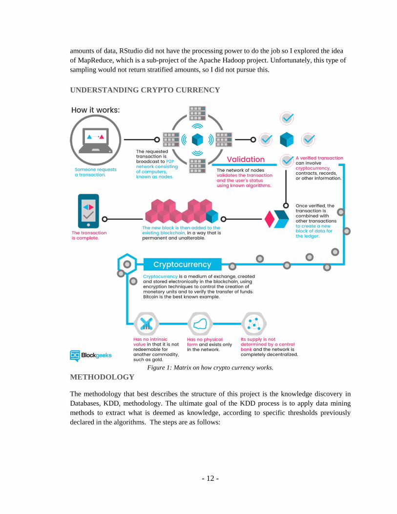
UNDERSTANDING CRYPTO CURRENCY
Figure 1: Matrix on how crypto currency works.
METHODOLOGY
The methodology that best describes the structure of this project is the knowledge discovery in
Databases, KDD, methodology. The ultimate goal of the KDD process is to apply data mining
methods to extract what is deemed as knowledge, according to specific thresholds previously
declared in the algorithms. The steps are as follows:

- 13 -
Figure 2: KDD methodology steps outlined.
Selection
The first stage of the following the KDD process is the selection stage. This is the acquiring of
target dataset or datasets that will then be analysed to discover useful information about the
chosen topic. This step was a lot more difficult than I had anticipated. Although, the bitcoin
ledger is openly sourced online, I wanted to carry my analysis using R as my chosen language
which limited my selection of which datasets I could use. Kaggle was my first choice when
searching for datasets as I love the detail in which comes with the datasets from Kaggle. This data
consists of data from 23.02.2010 to 20.02.2018 and has many attributes which can consider
factors for affecting the price of bitcoin. We will explore this later when building our regression
model.
Bitcoin in a very technical concept to understand and it’s very important to understand the data
you are working with. After a lot of research, I decided to take a medium sized dataset from
Kaggle (Found here - https://www.kaggle.com/sudalairajkumar/cryptocurrencypricehistory/data).
The dimensions can be seen below. This data set was formatted in a .csv file. As I finished my
analysis on this dataset, I felt comfortable and confident to move onto bigger data. I acquired
seven datasets (Found here -http://www.vo.elte.hu/bitcoin/downloads.htm) This data includes the
list of all transactions up to 28.12.2013. Dimensions can be seen below. All files from site were
downloaded as .txt files.
Figure 3: Dimensions of the dataset from Kaggle.
Figure 4: Dimensions of each dataset from the ELTE site loaded into RStudio. Total 7 datasets.

- 14 -
Pre-processing
The next step is to pre-process my data. Considerably, this stage is deemed most important and can
have a significant effect on your model’s performance. This process was a smoothed with the
Kaggle due to the size. In fact, the entire pre-processing stage with this dataset was relatively quick
and easy. The basic read.csv function was used to read in this file. This step involves the removal
of noise, outliers, collection of necessary information to build your model and strategies for
handling missing fields of data. Luckily by applying the is.na(x) function to all datasets, no ‘TRUE’
values were returned, indicating no null values.
The anytime library in R was installed and loaded to convert the timestamp. This was then formatted
using the as.Date method in R. An additional column was added for s count of days for each row.
These changes can be seen in figure 3 and 4.
Figure 5: Timestamp conversion
Figure 6: adding columns and formatting date
Transformation
This stage was not needed for the Kaggle bitcoin set. After my ELTE datasets was pre-processed,
I began the transformation process. Firstly, I had to sample my data as the sizes were extremely
large and there were no resources available to handle that amount of data. I then came to learn
about fread function which is an extension of the data.table library in R. This helped
tremendously with runtime and eventually loaded all seven datasets into the one session in R. I
then began my sampling process, which led to dimension reduction on all rows so they were
equal and manipulated into one data frame.
Data Mining
The data mining stage of the KDD process involves deciding which goal I want to reach with my
data and choosing the best model to showcase that goal. Ultimately, I want to gain as much
knowledge as I can from my dataset. I also want to be able to detect outliers and showcase important
patterns in my data as this will serve as very interesting information for an accountant. I have chosen
to build a regression and clustering model to do this.
The Kaggle bitcoin dataset is extremely informative in terms of market value, share etc. This will
be perfect to use when building my regression model. I can analyse the relationship among variables
and look at the market of bitcoin as a crypto currency as whole, and not just from a transactional
point of view. Is it worth investing in? What was the highest value of 1BTC? What was the lowest?
Does x effect the price of Y? Is x decreasing in value wile y rises in value? Is my data normal?
These, along with many more, are all questions a linear model can answer.

- 15 -
Figure 7. Example of a Linear Regression model predicting the price of bitcoin over time
Clustering is a great way to detect anomalies in your data. Those that don’t fit in with your data are
visually recognizable as outliers on your graph. Clustering is also a great way to visual your data
and classify it. For this analysis, I have chosen to apply the k-means clustering algorithm. K-means
is a type of unsupervised learning with the goals of grouping the data based on certain criteria’s.
The number of groups are represented by the number K. The algorithm works iteratively to assign
each point to one of the K groups based on the features provided. This is based on the similarity of
your data points as to where cluster it belongs to. Choosing K can be very difficult when you do
not have pre -defined classes in your data. This will be a challenge for this project.
Figure 8: Example of a K means cluster on a 2D graph in R where K=3.
Interpretation/Evaluation
After my models have been built. I will run my data through them to see the results. Based on the
results, I will visually represent my findings via tableau and graphs created in R. This allows for
easier interpretation for those less technical minded and an easier comparison when I am referring
back to the idea behind this project, which is the power of analytics vs. accountancy.

- 16 -
ANALYSIS & DESIGN
USE CASES
Figure 9: Use Case for this project
DATA REQUIREMENTS
The below datasets were required to complete my analysis. They were taking from Kaggle and the
ELTE bitcoin project website. The timeframe is from 10th November 2009 until 7th November 2017.
The Kaggle dataset has 2921 rows and 21 columns, whilst the other datasets combined have a total
of 254,495,928 rows and 20 columns. The features of the datasets are split as follows:
Kaggle provided the dataset regarding the bitcoins transactions.
https://www.kaggle.com/sudalairajkumar/cryptocurrencypricehistory/data
Date: Date of observation
btc_market_price: Average USD market price across major bitcoin exchanges.
btc_total_bitcoins: The total number of bitcoins that have already been mined.
btc_market_cap: The total USD value of bitcoin supply in circulation.
btc_trade_volume: The total USD value of trading volume on major bitcoin exchanges.
btc_blocks_size: The total size of all block headers and transactions.
btc_avg_block_size: The average block size in MB.

- 17 -
btc_n_orphaned_blocks: The total number of blocks mined but ultimately not attached to the
main Bitcoin blockchain.
btc_n_transactions_per_block: The average number of transactions per block.
btc_median_confirmation_time: The median time for a transaction to be accepted into a
mined block.
btc_hash_rate: The estimated number of tera hashes per second the Bitcoin network is
performing.
btc_difficulty: A relative measure of how difficult it is to find a new block.
btc_miners_revenue: Total value of coinbase block rewards and transaction fees paid to
miners.
btc_transaction_fees: The total value of all transaction fees paid to miners.
btc_cost_per_transaction_percent: miners revenue as percentage of the transaction volume.
btc_cost_per_transaction: miners revenue divided by the number of transactions.
btc_n_unique_addresses: The total number of unique addresses used on the Bitcoin
blockchain.
btc_n_transactions: The number of daily confirmed Bitcoin transactions.
btc_n_transactions_total: Total number of transactions.
btc_n_transactions_excluding_popular: The total number of Bitcoin transactions, excluding
the 100 most popular addresses.
btc_n_transactions_excluding_chains_longer_than_100: The total number of Bitcoin
transactions per day excluding long transaction chains.
btc_output_volume: The total value of all transaction outputs per day.
btc_estimated_transaction_volume: The total estimated value of transactions on the Bitcoin
blockchain.
btc_estimated_transaction_volume_usd: The estimated transaction value in USD value.
ELTE Bitcoin Project website and resources provided the below datasets.
http://www.vo.elte.hu/bitcoin/zipdescription.htm
blockhash.txt -- enumeration of all blocks in the blockchain, 277443 rows, 4 columns:
blockID -- id used in this database (0 -- 277442, continous)
bhash -- block hash (identifier in the blockchain, 64 hex characters)
btime -- creation time (from the blockchain)
txs -- number of transactions
txhash.txt -- transaction ID and hash pairs, 30048983 rows, 2 columns:
txID -- id used in this database (0 -- 30048982, continous)
txhash -- transaction hash used in the blockchain (64 hex characters)

- 18 -
addresses.txt -- BitCoin address IDs, 24618959 rows, 2 columns:
addrID -- id used in this database (0 -- 24618958, continous, the address with addrID ==
0 is invalid /blank, not used/)
addr -- string representation of the address (alphanumeric, maximum 35 characters; note
that the IDs are NOT ordered by the addr in any way)
tx.txt -- enumaration of all transactions, 30048983 rows, 4 columns:
txID -- transaction ID (from the txhash.txt file)
blockID -- block ID (from the blockhash.txt file)
n_inputs -- number of inputs
n_outputs -- number of outputs
txin.txt -- list of all transaction inputs (sums sent by the users), 65714232 rows, 3 columns:
txID -- transaction ID (from the txhash.txt file)
addrID -- sending address (from the addresses.txt file)
value -- sum in Satoshis (1e-8 BTC -- note that the value can be over 2^32, use 64-bit
integers when parsing)
txout.txt -- list of all transaction outputs (sums received by the users), 73738345 rows, 3 columns:
txID -- transaction ID (from the txhash.txt file)
addrID -- receiving address (from the addresses.txt file)
value -- sum in Satoshis (1e-8 BTC -- note that the value can be over 2^32, use 64-bit
integers when parsing)
txtime.txt -- transaction timestamps (obtained from the blockchain.info site), 30048983 rows, 2
columns:
txID -- transaction ID (from the txhash.txt file)
unixtime -- unix timestamp (seconds since 1970-01-01)

- 19 -
IMPLEMENTATION
In this section, the main parts of the code will be explained using code snippets where appropriate.
The majority of code was developed and tested using RStudio
SET UP THE ENVIRONMENT
Firstly, we need to set our working directory, so all files loaded are coming and going to the one
folder. Next, we need to tell R environment which libraries will be used during the script. All R
packages are first installed into libraries, which are directories in the file system containing a
subdirectory for each package installed there. Then every time you open RStudio, you need to load
the library function for each library, so R knows which libraries you are using on that script. This
can be seen below. Now the data is ready to be read in and your analysis can begin.
Figure 10: Setting up R environment
CLEANING THE DATA
The Kaggle dataset was relatively small, so a simple view() function in RStudio can allow for some
visualisation on the data to check for any null values. Alternatively, on our much larger datasets, I
applied a is.na(x) function and luckily no NULL’s were found. Other pre-processing steps including
renaming of columns for easier reading, removal of similar columns among the datasets before the
transformation stage could begin. Unix Timestamp was converted and changed into date format.

- 20 -
Figure 11: Renaming of columns for easier analysis
Our Kaggle dataset variable, btc_median_confirmation_time, had a lot of ‘0’ values. This could
cause our data to have a skewered distribution and for our data to appear not normal. To avoid this,
I created a subset which only includes instances greater than 0 for this variable. When I am
comparing and analysing this variable, I will query my subset dataset, BitcoinData2.
Figure 12: creating a subset of data that is clean
SAMPLING THE DATA
Each dataset was individually read into RStudio.
The ELTE datasets (all 7) are massive in size so the reading process alone took hours. This was
down to lack of computational power. However, my machine is less than a year old and has 8GB
RAM and struggled immensely with handling this data so that highlights the volume of data that
was processed. After a lot of restarting RStudio and machine, and a lot of unresponsive programs,
I began experimenting with different packages in R that helps handle big data. Eventually I learnt
of the fread() function which is a method from the Data.Table package. (This saved my day!)
Fread is capable of reading in large amount of data and even gives a status report after it has been
read as to how long it took and how much data was read. Also, whilst the data is being read, there
is a percentage progress bar which shows you how much of the data has been read. A feature in
which RStudio is lacking in itself, if I may add.
In Figure 5 you will see the time in which it took to read in some of the datasets. Figure 6
highlights even with a big memory function applied, the read time can still be very long when
dealing with huge amounts of data. These datasets had to be read in numerous of times at the
beginning until eventually RStudio and my machine worked up the processing power to read all 7
datasets in the one session. There were a lot of trial and error and a lot of time spent on this step
before I could process to the next stages.

- 21 -
Figure 13: The fread function reading in 3 of the 7 larges datasets
Figure 14: shows the time in which it took to read in one of the biggest datasets out of the 7. Almost 49
minutes!
Using another R method, sample(), I was able to specify how many samples I wanted from my set
and apply different probabilities for each sample. I decided to split my data into train and test sets.
The training set can be used when building my model and the test set can be used when my model
is complete for testing purposes. After my data was sampled, I then wrote the two individual
samples (test and train) to separate .csv files. This was so I would not have to spend the time reading
in the entire datasets again and sampling them each time. This process was repeated for all seven
datasets.
Figure 15: txhash.txt dataset being read in, sampled, split into two sets then read individually to two .csv
files.
DIMENSION REDUCTION
FROM THIS
TO THIS

- 22 -
Figure 16: Dimension reduction on all training sets.
Once the seven datasets were successfully split into training and test sets. I rebooted R and only
loaded in all the training sets. They were all of different dimensions, so I applied a dimension
reduction method on the rows of each set and matched the size to that of the smallest train set,
which was (btc_output 74047). This was the quickest most efficient way to reduce my data is size
to all match so that they could then be combined into one data frame.
COMBINING THE DATA & BUILDING A DATA FRAME
The below code snippets show the steps in which I took to combine my seven training sets into one
data frame. Once the row dimensions in all sets were equal, it was easy to then combine the data in
the one frame using the data.frame() function in R.
Figure 17: combining train sets into a data frame
I then wrote the data frame to a .csv file so that I could not have to load the above code every time I want to
analyse my data frame. This was a much easier option for going forward with the project. Also, my datasets
have finally been condensed to a manageable size and I could view my data as a whole in excel. This also

- 23 -
showed me there were a lot of duplicate ‘ID’ attributes which needed to be removed. For ease of use, I did
this in a matter of seconds in excel.
ANALYZING AND EXPLORING THE DATA
The first step I always take in exploring my data is to run the summary command. This command
is so simple yet so powerful in summarizing your data. You get results in a matter of seconds which
is a great thing about R as a language. Below we can see some interesting things about our data
frame, the mean number of inputs are 0.52 and the mean number of outputs are 1.168. This shows
there is a greater amount of transactions being sent than received, which makes sense really!
Although, these numbers are extremely small. This could be down to the security measures behind
the blockchain which provide each transaction with a unique address, making it hard to trace back
to the seller, so again making it difficult to determine exactly how many transactions have come
from the same seller.
Figure 18: summary command in RStudio on df
I separately ran a command to get the average time as it was in Unix and I wanted the time as
well as the date displayed. By using the anytime() library in R this was done and can be seen
below.
Figure 19: Mean time of transactions

- 24 -
Below is a code snippet on the code I ran to display a correlation matrix of my Kaggle dataset. I
felt this would be very interesting considering the attributes in this set. A correlation matrix
displays, usually in a percentage, the relationship among two variables. In this case, my variables
are my attributes. A score close to 1 displays a strong relationship among variables x and y. A
score near .5 displays a medium relationship among x and y variables. Anything below would be
considered weak.
Figure 30: code snippet from RStudio of correlation matrix
For easier reading, I worded my column names before displays the correlations as a matrix.
Below you can see a thermostat output of the relationship among variables. The darker the blue,
the stronger the relationship. The whiter the colour, then we would conclude a medium
relationship. Then we can look at any red as the “danger zone” concluding an extremely weak
correlation and no relationship. It is clear to see there is a lot bluer tones, showing a lot of strong
relationships. There are absolutely no red tones but a lot of white tones. White tones indicated a
correlation coefficient close to 0 which signifies that there is no linear relationship between the
variables. This matrix is a good indicator to analyse when building a model as it specifies which
variables have an impact on one another.
Figure 21: Correlation Matrix

- 25 -
MarketPrice and MarketCap have a correlation coefficient of 0.99. This is extremely high
showing a strong relationship. This makes sense as generally market caps do have an effect on
market price.
BTCDifficulty, HashRate, MinersRevenue, EstTransactionVolUSD are also all highly correlated
with MarketPrice with coefficients of .9+.
OutputVolume, and TotalBTC have low correlations with MarketPrice suggesting they do not
contribute to one another.
VISUALIZING THE DATA
The next step was to visualise my data. This step only makes sense after you have done enough
research to understand your data. Otherwise it would be too difficult to comprehend the graphs.
A common question to ask about the strength of any currency, is it getting stronger or weaker over
time? The graph to the left represents our Kaggle data which clearly shows the value of bitcoin is
getting higher as time progresses. The right graph represents our transactional dataset, ELTE, and
shows the number of transactions being sent are relatively small and don’t seem to be increasing as
time goes on too much. This could suggest users are more inclined to receives bitcoins but not send
them.
Figure 22: ggplot from R. Left image is Kaggle data and right is ELTE data.
Below I plotted bitcoins market capitalization which is the total USD value of bitcoin supply in
circulation versus the Market Price (Average USD market price across major bitcoin exchanges).
The data points were graphed onto a linear model. Linear regression attempts to model the
relationship between two variables by fitting a linear equation to observed data. Additionally, we
can see our datapoints are all on the linear regression line which shows our data is normal. It is
clear to see that both variables are dependent on one another. As market price rights so does
Market capitalization and visa versa. I referred back to my correlation matrix and seen a
coefficient of 0.99 between them which confirms this.

- 26 -
Figure 23: ggplot of Market Capitalization vs. Market Price
Figure 24: ggplot of Market Capitalization vs. Market Price
BUILDING THE MODELS
In statistics, linear regression is an approach at modelling the relationship between a dependent
variable y and one or more explanatory variables (or independent variables) denoted X.
Market Price vs. Estimated Transaction Volume Linear Model
t value Pr(>|t|)
----------------------------------------------------------- --------- ----------
**poly(BitcoinData2$btc_estimated_transaction_volume_usd, 168 0
2)1**
**poly(BitcoinData2$btc_estimated_transaction_volume_usd, -15 5.5e-50
2)2**

- 27 -
**(Intercept)** 76 0
--------------------------------------------------------------------------------
The t statistic is the coefficient divided by its standard error. The standard error is an estimate of
the standard deviation of the coefficient, the amount it varies across cases. It can be thought of as
a measure of the precision with which the regression coefficient is measured.
> lm1 <- plot(BitcoinData2$btc_market_price~ BitcoinData2$btc_estimated_transaction_volume_usd) > meanlm1 <- mean(BitcoinData2$btc_market_price) > abline(h=meanlm1) > R2=summary(lmfit2)$r.squared > cat("R-Squared =", R2) R-Squared = 0.9262094
R- Squared, also known as the coefficient of determination, is the proportion of variability in y that
is explained by the independent variable, x, in the model.
Our independent x variable is btc_estimated_transaction_volume_usd and our dependent variable
y is btc_market_price. Our R-Squared value tells us that 92% of bitcoins market price is due to
bitcoins estimated volume of transactions. Although this value of R-Squared is high, the x and y
variables by themselves or together, do not tell us enough about our data.
Figure 25: Graph of the residuals of lmfit2b
These plots exhibit “heteroscedasticity”, meaning that the residuals get larger as the prediction
moves from small to large (or from large to small). There appears to be a pattern in the residuals
plot above starting at zero and increasing linearly to approximately 1000 on the x-axis. Also
meaning as the price increases the variability increases. One way to remedy this may be to
transform a variable in the model. This will be considered when selecting variables for a
regression model.
- 28 -
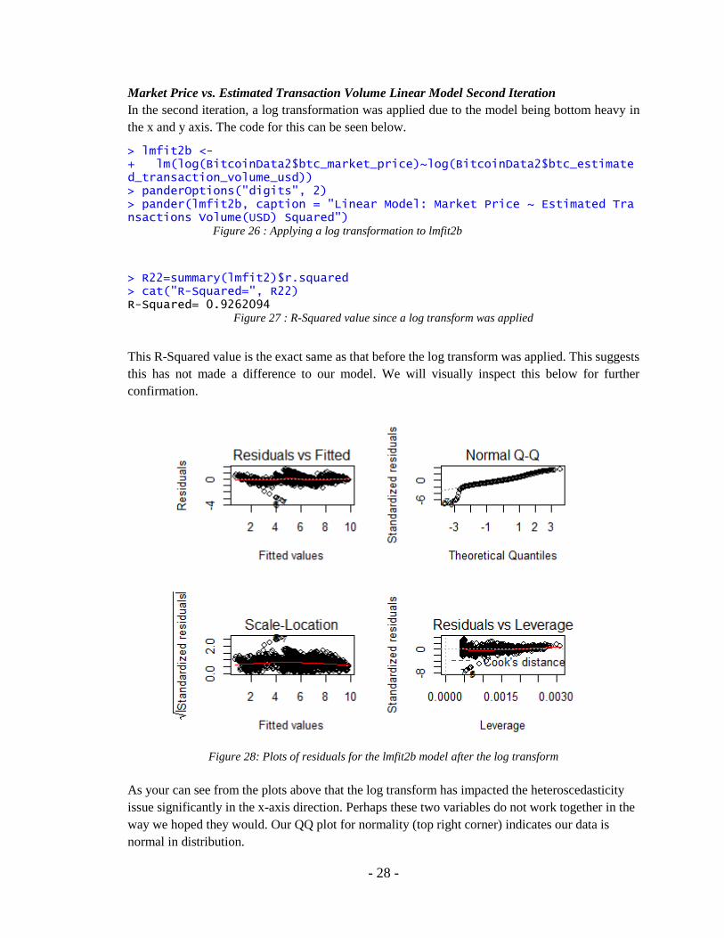
Market Price vs. Estimated Transaction Volume Linear Model Second Iteration
In the second iteration, a log transformation was applied due to the model being bottom heavy in
the x and y axis. The code for this can be seen below.
> lmfit2b <- + lm(log(BitcoinData2$btc_market_price)~log(BitcoinData2$btc_estimated_transaction_volume_usd)) > panderOptions("digits", 2) > pander(lmfit2b, caption = "Linear Model: Market Price ~ Estimated Transactions Volume(USD) Squared") Figure 26 : Applying a log transformation to lmfit2b
> R22=summary(lmfit2)$r.squared > cat("R-Squared=", R22) R-Squared= 0.9262094
Figure 27 : R-Squared value since a log transform was applied
This R-Squared value is the exact same as that before the log transform was applied. This suggests
this has not made a difference to our model. We will visually inspect this below for further
confirmation.
Figure 28: Plots of residuals for the lmfit2b model after the log transform
As your can see from the plots above that the log transform has impacted the heteroscedasticity
issue significantly in the x-axis direction. Perhaps these two variables do not work together in the
way we hoped they would. Our QQ plot for normality (top right corner) indicates our data is
normal in distribution.

- 29 -
Market Price vs. Miners Revenue Linear Regression Model
A linear model was built to see whether there was a relationship between the market price of bitcoin
and the miners revenue. The miners revenue is the total value of coinbase block rewards and
transaction fees paid to miners. The market price is based on the average USD market price across
major bitcoin exchanges. The output is as follows:
> lmfit3<-lm(BitcoinData2$btc_market_price~poly(BitcoinData2$btc_miners_revenue
,2))
> panderOptions("digits", 2)
> pander(lmfit3, caption = "Linear Model: Market Price ~ Miners Revenue (USD) S
quared")
---------------------------------------------------------------------------
Estimate Std. Error t value
----------------------------------------- ---------- ------------ ---------
**poly(BitcoinData2$btc_miners_revenue, 125159 375 334
2)1**
**poly(BitcoinData2$btc_miners_revenue, -12954 375 -35
2)2**
**(Intercept)** 1152 7.9 147
---------------------------------------------------------------------------
Table: Linear Model: Market Price ~ Miners Revenue (USD) Squared (continued bel
ow)
----------------------------------------------------
Pr(>|t|)
----------------------------------------- ----------
**poly(BitcoinData2$btc_miners_revenue, 0
2)1**
**poly(BitcoinData2$btc_miners_revenue, 7.8e-211
2)2**
**(Intercept)** 0
----------------------------------------------------
> R3=summary(lmfit3)$r.squared
> cat("R-Squared = ", R3)
R-Squared = 0.9802747
Figure 29: Code output of our linear model for comparing the relationship between bitcoins market price
and bitcoins Miners revenue.
R-Squared value indicates that 98% of our market price is due to Miners Revenue.

- 30 -
Figure 30: Residuals vs Fitted for lmfit3. I have circled possible outliers.
Again, there are signs of heteroscedasticity. Also, we can see a lot of our data have formed into
clusters. This graph clearly indicates there are outliers in our data. This could be a factor in our
graph having dispersions. Perhaps a very large or very small data point far from the mean have
caused our data to appear this way. This graph highlights how versatile regression is as data
mining method. It is a great visualisation method for viewing your data and checking for
anomalies. I have circled these above. This fits very well with my project.
Market Price vs. Block Find Difficulty Linear Model
Next, we look at a relative measure of how difficult it is to find a new block in the blockchain and
consider whether this has an effect on the market price.
This graph is really interesting. There is a lot of variance around the linear but the graph is still a
good indicator that there is a linear relationship in the data. Our R value can help with determining
this as sometimes we cannot say visually. Again, we can see some outliers among our data which
could be worth investigating.

- 31 -
> R5=summary(lmfit5)$r.squared > cat("R-Squared = ", R5) R-Squared = 0.8129002
There is an 81% chance that the block find difficulty has an effect on the market price.
Market Price vs. Hash Rate Linear Model
The linear model below represents the relationship between bitcoins hash rate and market price.
There is an 81% chance that the model explains all the variability of the response data around the
mean.
> R5=summary(lmfit5)$r.squared > cat("R-Squared = ", R5) R-Squared = 0.8129002
Figure 31
There are signs of some heteroscedasticity, but residuals are relatively flat. Evidence of some
obvious outliers can be seen in the graph to the left above. This is an indicator of possible
anomalous behaviour that can be skewing our data. In regression, outliers are known as
influential points. This is because an outlier greatly affects(influences) the slope of the regression
line. Our coefficient of determination is 81%. Due to evidence of outliers, we can assume our R-
squared value has been affected by these resulting in it being bigger or smaller
Market Price vs. All Variables
Now its time to look at all variables as a whole and how these are significant to the market price.
> pander(lmBTCm, caption = "Linear Model: Market Price vs. All Variable
s") (Output can be seen in the Appendix for this function, includes estimate, standard error, t-va
lue and p-value for all variables.)

- 32 -
Figure 32 residuals of all variables versus market price.
What’s really interesting to see from the graph is the number out outliers. By changing the pch to
1, this has become a lot clearer and easier identifiable.
We can also see that the majority of the volume is located in the lower x-axis region. Our data see
ms to be very clustered around this region. In general, the trend line is relatively flat.
Now we look at the relationship between market price and our highly correlated variables only.
Figure 33
We have an extremely high R-squared value. This suggests our model is doing a good job. It
appears our highly correlated variables are significant to the market price. Our trend line is not
very flat nor is our data evenly dispersed.
If we condense our variables further, this may have a positive impact. Market Capitalization and
Estimated Transaction Volume are highly correlated, only one will be included in the model.
Also, because Difficulty and Hash Rate are highly correlated, the model will only include one.
> cat("R-Squared = ", Rb6)
R-Squared = 0.9736494

- 33 -
Figure 34
Still some heteroscedasticity, but the best model so far.
Polynomial Multivariable introduced to "Linear Model: Market Price ~ Miners Revenue
Squared + Count of Transactions Squared" linear model
Polynomial regression is a special case of multiple linear regression when the relationship between
the independent variable x and dependent variable y is modelled as a nth degree polynomial in x.
Our R-squared value is extremely high in comparison with the non-polynomial multivariable
regression.
Figure 34
With polynomials introduced, we can see our graph does not have as much dispersion as
recommended and it also results in a flatter line. We can consider this model, the best thus far.
Now its time to train the model and test it
For this model I will use the same model features as above for lmfit7.
> set.seed(1)
> train.index<-sample(1:nrow(BitcoinData2),0.80*nrow(BitcoinData2), replace=FAL
SE)

- 34 -
> train <- BitcoinData2[train.index, ]
> test <- BitcoinData2[-train.index,]
> lmtrain <- lm(btc_market_price~poly(btc_estimated_transaction_volume_usd,2) +
poly(btc_miners_revenue,2) , train)
> test$p1 <- predict(lmtrain,test)
Figure 36: Splitting the data into training and testing
> ggplot(test, aes(test$Days)) +
+ geom_point(aes(y=test$btc_market_price),color="red") +
+ geom_line(aes(y=test$p1), color="Blue")+
+ ggtitle('BTC Prediction vs. Actuals') +
+ theme(plot.title = element_text(size=16, face="bold",
+ margin = margin(10, 0, 10, 0)))+
+ labs(x="Days", y="Market Price (USD)")+
+ theme(axis.text.x=element_text(angle=90, vjust=0.5)) +
+ theme(panel.background = element_rect(fill = 'grey75'))+
+ labs(title = paste("BTC Linear Regression Model Prediction vs. Actuals",
+ "\n\nAdj R2 = ",signif(summary(lmtrain)$adj.r.squared, 5
),
+ " P =",signif(summary(lmtrain)$coef[2,4], 2)))
Figure 37: Output for the above code snippet
We can see the model does a great job at tracking the test set. If we add a column for the percenta
ge of change for the market price this is our output…. (this was done using the mutate() and lag()
function.)

- 35 -
Figure 38: Bitcoin market price percentage of change over time
Figure 39 : The code snippet for the above output.
As you can see from the code snippet above, I used the library zoo in R to transform the variables
to percentages by multiplying 100 by each variable. I then created another correlation matrix
based on the transformed variables.

- 36 -
Figure 40: Correlation Matrix output in R on transformed variables.
We can see from our matrix, the percent in market price is highly correlated with the percent change
in market capitalization.
"Linear Model: Market Price Change ~ Market Cap Change + Total Coins Change"
Creating a linear model of the percent of market price change versus market cap change plus the
total number of coins change. Our model is extremely flat with a very even distribution. There are
some obvious outliers which I have circled orange. Not only is this the best model yet, but we
have found a model which displays our outliers very clearly. Again, highlight the versatility and
power of a good regression model! Now its time to test our model.
Figure 41: Testing and training our model

- 37 -
Thankfully we have a relatively small amount of error when train and test our model. Below is a
visualization of the final model. From the above implementation, we have learnt it is better to
create a model based on percent change. As prices rise, so does a lot of associations with the
value of currencies such as market capitalization, miners revenue etc. Otherwise, our models were
showing a lot of heteroscedasticity in a non-zero scenario.
Figure 42: Final Model Representation
We now know, percent change in the value of Bitcoin is highly dependent to the percent change
in Market Capitalization and percent change in total bitcoins in Circulation. This makes a lot of
sense as how can you make money from bitcoins that are not available?!
#sources include: http://www.statisticssolutions.com/conduct-interpret-linear-regression/,
https://www.kaggle.com/sudalairajkumar/cryptocurrencypricehistory, http://www.vo.elte.hu/bitcoin/zipdescription.htm
https://www.kaggle.com/alisaaleksanyan/prediction-of-bitcoin-price-linear-regression/code

- 38 -
TESTING
The data analysis throughout this process consisted of sampling large amounts of data,
manipulating data frames and reading data from comma separated and text files. A function as
created using one of RStudio’s assertr packages to conduct a test to test the output of a given data
frame.
data <- read.csv("bitcoin_dataset.csv")
data %>%
assertr::verify(nrow(.)>2919)
...
Figure 43 : Function Testing the output of a Data Frame
The function above is expects that in the data frame there is greater than 2919 rows. The function
returns no error’s, so it is successful.
> data %>%
+ assertr::verify(nrow(.)>2921)
Error in assertr::verify(., nrow(.) > 2920) :
verification failed! (1 failure)
Figure 44: Error occurring in function when number of rows is greater than expected
Above is an example of the function displaying an error. There are 2920 observations in the data
frame and the function was manipulated to test for more than this amount which return an error.
Unit testing: Programmatic tests that evaluate a unit of your code at a low level. These tests are
small bits of code that can often be automated. East test was conducted in RStudio using the
testthat package. You can see the code for this below.
library(testthat)
source('C:/Users/paris/Desktop/College/College/Paris Moore Software
Project/Code/test_Regression.R')
test_results <- test_dir("C:/Users/paris/Desktop/College/College/Paris Moore Software
Project/Code/test.R", filter = NULL, reporter="summary"

- 39 -
CONCLUSION & FURTHER WORK
To conclude this analysis, I have created a matrix below of a list of technical and non-technical
skills, associated with auditing and accounts. Followed by a column for Analytics and a column for
Accountants. This is a comparison table of skills for both parties.
Figure 45: Comparison table of skills of an accountant vs. analytics person
As you can see, there isn’t a lot that an accountant is lacking in comparison to that of an analytic
minded person. However, if we were to add a constraint to this table, such as carrying out the
above task in less than a matter of minutes, the accountant’s columns would consist of nothing
but red X’s, whilst the analytics column would look the same as it does now. Additionally, if we
were to add constraints based on complexity such as data size, again, we would suspect the
accountant would struggle a lot more/take a lot longer than that of an analytic mindset. My
comparison is not suggesting in any way that an analytic minded person is “smarter” than an
accountant, but the resources and skillset a data analyst holds is much more powerful in
conducting the above tasks. Also, during my analysis I was constantly comparing the work load
between the two and realised the limits to which each can go. I understand an accountants job has
digitally transformed the past decade, in line with technology evolving. However, the point I have
learnt is, how powerful is taking someone else’s output and interpreting it yourself versus
someone who creates the output, manipulates it until the optimized output is achieved? Also, how
much can you rely on a computer program to continuously run commands over and over again
without missing any “unusual” noise? Would this risk be better managed and reduced by a more
technical minded person running the programs with a complete understanding of what is going on
in the background? These are many questions I have begin asking myself since carrying out my
analysis.

- 40 -
Additionally, my linear regression implementation has opened my eyes immensely at the
power of this data mining tool alone. I began this project with the idea of applying clustering to
my data as it seemed like the most obvious solution in detecting outliers, but that was the
problem, it was too “obvious”. It did not align in with auditing transactions, where as regression
allowed for a full analysis on the bitcoin market. I was really intrigued by the fluctuation in the
market price of bitcoin that I wanted to figure out which variables impacted this the most. Along
the way, it became clear that linear regression was a lot more than a relationship among two
variables (my initial understanding). It allowed for outlier detection as well as being able to
determine if your data was normal and how it was distributed. Dealing with large amounts of data
is difficult in all aspects, but plotting your data using linear regression made this a lot easier and
allowed me to fully understand my data and decide on my end result.
As I just outlined, big data – how I underestimated this. The sampling phase of the ELTE
datasets was by far the most complicated and time-consuming part of this project. Whether this
was down to computational power I am still unsure. RStudio definitely struggled with this phase
as much as I did. Nevertheless, my knowledge, respect and handling of big data has definitely
grown throughout this project.
To finally summarise this report, I refer back to my first question, “Can data analytic’s
shape the work of accountants?”, personally I say 100% it can. The knowledge defined within the
huge volumes of data processed every second of everyday is never ending. People like
accountants who work with data day in and day out, are being relied on by companies to report
back as much information as they can from the data, this cannot be done without the necessary
tools and skillset of that of a data analyst.
Final Thoughts
Overall this project has been of huge interest and an exceptional learning curve. I began this project
not know what Bitcoin nor the blockchain was and have soon become, what feels like, an expert in
the area. (not really!) A special thank you to all who contributed towards this project. An extra
special thanks to my Supervisor, Simon, for having the patience of a saint and guiding me from
start to finish with this. A final thanks to the staff at the National College of Ireland for teaching
me to progress to this level over the last four years. It’s been a pleasure.

- 41 -
APPENDIX
SUPERVISOR INTERACTION
4th year Template – Learning Agreement/Minutes
Student Name Paris Moore
Student Number X14485758
Course BSc Computing
Project Title Auditing Crypto Currency Transactions, Anomaly Detection in Bitcoin
Overview of Project Looking for ways in which analytics can shape the work of accountants was the initial idea of this project. When the question was proposed as to which dataset I could acquire to carry out my analysis, the idea of using the world’s leading crypto-currency’s bitcoin ledger posed as a great solution and one that would add flavour to my project.
Meeting 1
Date 16th November 2017
Time 10:00am
Duration of Meeting 30 minutes
Current Challenges Discuss November Technical Report. Which bitcoin dataset to use. Size, interpretation and complexity all play a pivot role.
Goals of Meeting: I had previously spoken to Simon about my final year project. He had some great insight and idea into my idea and I want to elaborate on it with him to get more guidance for my final report. I also have questions on which dataset I should be using and what type i.e. .csv, API etc.
Goals/Actions for next Meeting: Explore the idea of anomaly detection in more detail. Which methodology to follow. Size of the dataset which is required and whether I need multiple data sources.
Learning Agreement Student Signature
PARIS MOORE
Meeting 2
Date 13th February 2018
Time 13:30pm
Duration of Meeting 30 minutes

- 42 -
Current Challenges Still undecided on what data to use. Which anomaly detection method would be best.
Goals of Meeting: Simon has helped me find a site online which has several versions of bitcoin datasets. The dimensions are massive. There are seven datasets in total. Simon kindly provided me which his clustering tutorial for his master students. This should assist with my understanding of k-means clustering for anomaly detection.
Goals/Actions for next Meeting: Right now, there is no specific goal for the next meeting. However, we have scheduled to meet every Wednesday at 1:30pm going forth.
Learning Agreement Student Signature
PARIS MOORE
Meeting 3
Date 2nd May 2018
Time 3:30pm
Duration of Meeting 45 minutes
Current Challenges I am still unsure whether I can handle the volume of data I have. I am considering totally changing my data source and using google bigQuery API to pull data using Python.
Goals of Meeting: Discuss bigQuery Idea. Ask about technical report.
Goals/Actions for next Meeting: Ensure my data is successfully sampled, hopefully have all models built and I am ready to move onto the technical document.
Learning Agreement Student Signature
PARIS MOORE
Meeting 4
Date 9th May 2015
Time 2pm
Duration of Meeting 45 minutes
Current Challenges The biggest challenge I am facing is whether I have the technical ability to produce a k-means clustering model for anomaly detection by Submission on Sunday.
Goals of Meeting:

- 43 -
Discuss K-means. Look at grading rubric. Ask about presentation and second marker. Discuss what is left to do to produce a good project. Get tips and hints.
Goals/Actions for next Meeting: This could possible be my last meeting with Simon. However it has been said that it may be possible to meet next week to discuss the presentations.
Learning Agreement Student Signature
PARIS MOORE
PROJECT PROPOSAL
Objectives
The objective for this project is to specify, design, implement and document a medium to large
scale project in the chosen area of specialization. My chosen area of specialization is Data
Analytics. I am expected to choose a dataset from an area of interest and using Analytics tools and
techniques, inspect, extract and clean this data. I will further investigate my dataset to draw
conclusions about my data based on the areas I choose to investigate. The dataset I have chosen is
the online bitcoin ledger. Bitcoin is a worldwide cryptocurrency and digital payment system called
the first decentralized digital currency. I will inspect this dataset using the R programming language
and RStudio as my chosen software. I will investigate the anomalies in this dataset and try to draw
some conclusions around these bitcoin transactions. Also, as part of this project I will also look for
ways to implement data analytics within Accountancy. I will use the bitcoin ledger as my dataset
for this and audit crypto currency transactions and investigate for any anomalies.
During the cycle of this project, I will look at ways of improving and enhancing my developing and
presentation skills. I will communicate monthly with my supervisor and work on my project
continuously referring to a strict project plan. I will draft up a comprehensive requirement
specification document to help with the process of my project.

- 44 -
Motivation
The world of auditing is evolving. Digital transformation is transforming businesses and how they
operate. Through this, accountants and auditors have huge amounts of data and are looking for
more ways to optimize that data and draw out some conclusions/predictions to help benefit their
business. Data analytic methodologies have the power to focus on outliers and exceptions,
identifying the riskiest areas of the audit.
The massive volumes of data now available inside and outside companies, and the power of new
data analytics technologies, are fundamentally changing the audit. The general view is that big data
will have a dramatic impact on enhancing productivity, profits and risk management. But big data
in itself yields limited value until it has been processed and analysed.
Analytics is the process of analysing data with the objective of drawing meaningful conclusions.
Major companies and organizations have recognized the opportunity that big data and analytics
provide, and many are making significant investments to better understand the impact of these
capabilities on their businesses. One area where we see significant potential is in the transformation
of the audit.
Technical Approach
Data Analysis:
When analyzing the data, I will use a CRISP-DM approach:
Business understanding: This phase concentrates on making sure I understand the
project objectives and requirements from a business point of view. Then taking this
perspective and converting it into a data mining problem and designing a plan on how
to approach the problem and solve it.
Data understanding: This phase involves data collection and pre-processing. This
involves looking for data integrity, ensuring the data is of high quality and fits in with
the requirements for this project. In order to move onto the next phase, it is crucial I
understand my data at this point.
Data preparation: This phase involves preparing your data to the point where you
construct your final dataset. Tasks include table, record, and attribute selection, data
cleaning, construction of new attributes, and transformation of data for modelling
tools.
Modelling: Once you have your final dataset, you can begin applying various
modelling techniques.
Evaluation: This stage involves re-evaluating your steps and ensuring your model
meets your business objectives and requirements. You can re track back through
some phases if needs be until your model is at the standard required for deployment.
Deployment: This phase is how you decide to represent your model; this can be as
simple as generating a report or as complex as implementing a repeatable data mining
process. This will depend on customer’s needs.
Special resources required
As of this moment I require no special resources.

- 45 -
1. Clustering
Clustering is the process of partitioning a group of data points (m nodes in the graph) into a
small number of clusters. The goal is to assign a cluster to each data point. K-means is a
clustering method that aims to find positions of the clusters that minimize the distance from the
data points to the cluster. It does this through an algorithm. It firstly decides the number of
clusters and gives this number a value k. Then:
This algorithm will fit very well as it will visually represent my data in a way that will make
any outliers visually obvious. We first need to represent each node as a multi-dimensional
vector in the Euclidean space.
2. Depth-based Approaches Model-based
3. Deviation-based Approaches
4. Distance-based Approaches based Approaches
5. Density-based Approaches
6. High dimensional Approaches
Project Plan
Task Mode Task Name Duration Start Finish Predecessors Resource
Names
Manually
Scheduled
Project
Proposal
25 days Mon
18/09/17
Fri 22/10/17
Auto
Scheduled
Brainstorming
Project Ideas
5 days Mon
18/09/17
Fri 22/09/17
Auto
Scheduled
Lecturer for
feedback on
Idea
1 day Mon
25/09/17
Mon
25/09/17
2
Auto
Scheduled
Project Pitch 1 day Wed
04/10/17
Wed
04/10/17
Manually
Scheduled
First Monthly
Journal Entry
1 day Fri 06/10/17 Fri 06/10/17
Auto
Scheduled
Project
Proposal
Document
12 days Thu 05/10/17 Fri 20/10/17 4
Manually
Scheduled
Meeting with
Supervisor
1 day Tue 12/09/17 Tue 12/09/17
Manually
Scheduled
Meeting with
Supervisor
1 day Tue 19/09/17 Tue 19/09/17
Manually
Scheduled
Proof read
Project Proposal
Document and
Upload
1 day Fri 20/10/17 Fri 20/10/17

- 46 -
Manually
Scheduled
Requirement
Specification
15 days Mon
23/10/17
Fri 10/11/17
Auto
Scheduled
Acquire all data
sets for the
project
5 days Mon
23/10/17
Fri 27/10/17
Auto
Scheduled
Requirement
Specification
Document
15 days Mon
23/10/17
Fri 10/11/17
Manually
Scheduled
Meeting with
Supervisor
1 day Thu 02/11/17 Thu 02/11/17
Manually
Scheduled
Requirements
Specification
Review &
Upload
1 day Fri 10/11/17 Fri 10/11/17
Auto
Scheduled
Second
Monthly Journal
Entry
1 day Fri 03/11/17 Fri 03/11/17
Manually
Scheduled
Project
Prototype
25 days Sat 11/11/17 Thu
14/12/17
Manually
Scheduled
Data Cleansing 5 days Mon
06/11/17
Fri 10/11/17
Manually
Scheduled
Start to create
prototype for
Application in
Android Studio
14 days Sat 11/11/17 Wed
29/11/17
Manually
Scheduled
Meeting with
Supervisor
1 day Thu 16/11/17 Thu 16/11/17
Manually
Scheduled
Third Monthly
Report
1 day Fri 08/12/17 Fri 08/12/17
Manually
Scheduled
Mid-Point
Presentation
4 days Mon
11/12/17
Thu
14/12/17
Manually
Scheduled
Meeting with
Supervisor
1 day Thu 14/12/17 Thu 14/12/17
Manually
Scheduled
Finish
Prototype and
Prepare for
Presentation
Manually
Scheduled
Post Mid-Point
Presentation
31 days Mon
18/12/17
Mon
31/01/18
Manually
Scheduled
Process
feedback from
mid-point
presentation and
start to make
alterations
5 days Mon
18/12/17
Fri 22/12/17
Manually
Scheduled
Christmas
Break
5 days Sat 22/12/17 Thu 28/12/17
Manually
Scheduled
Fourth
Monthly Report
1 day Fri 29/12/17 Fri 29/12/17
Manually
Scheduled
Continue to
develop
prototype
10 days Mon
01/01/18
Fri 12/01/18
Manually
Scheduled
Meeting with
Supervisor
1 day Fri 26/01/18 Fri 26/01/18
Manually
Scheduled
Analyze
Datasets and
arrive to
conclusions
12 days Sat 13/01/18 Tue 30/01/18
Manually
Scheduled
Prepare Final
Working
Project
40 days Thur
01/02/18
Wed
28/03/18
Manually
Scheduled
Design my
Application
5 days Thur
01/02/18
Wed
07/02/18
Manually
Scheduled
Fifth Monthly
Report
1 day Sat 03/02/18 Sat 03/02/18
Manually
Scheduled
Meeting with
Supervisor to
discuss final
stages and
implementations
1 day Fri 09/02/18 Fri 09/02/18

- 47 -
Manually
Scheduled
Finish
Analysis of
datasets
17 days Thur
08/02/18
Fri 02/03/18
Manually
Scheduled
Completion of
application and
data analysis of
data-sets
14 days Fri 09/03/18 Wed
28/03/18
Manually
Scheduled
Testing 5 days Thur
29/03/18
Wed
04/04/18
Manually
Scheduled
Create and
Implement Test
Plans for final
Application
3 days Thur
29/03/18
Sat 31/03/18
Manually
Scheduled
Create and
Implement Test
Plans for
findings in data-
sets
3 days Sun 01/04/18 Wed
04/04/18
Manually
Scheduled
Final Report 31 days Thur
05/04/18
Thur
17/05/18
Manually
Scheduled
Prepare Final
Document
Manually
Scheduled
Upload
Software
1 day Thur
17/05/18
Thur
17/05/18
Manually
Scheduled
PROJECT RESTRICTIONS
Data
All transactions analysed will be historical data. This report acknowledges that bitcoins datasets
are all open source.
Time:
The project timeline spans from September 2017 until May 2018.
Cost:
The poster is a project requirement which will cost €20 to be printed.
Software:
Student resources and open source platforms provide the necessary tools. For the duration of this
project I have been working from my own machine.
Legal:
Datasets in relation to the bitcoin are open source and provided by the many sites online. For this
project, I will be using Kaggle, a platform for predictive modelling and analytics, to gather the
majority of my data. All data gathered will be referenced accordingly. An ethics form was also
filled out to ensure against data protection laws.
FUNCTIONAL/NON-FUNCTIONAL REQUIREMENTS
SECURITY REQUIREMENTS

- 48 -
Security is a fundamental aspect to the system. The data provided will be securely stored in local
disk and backed up to the cloud. The Data Administrator will have full rights and access to the
account and will only allow others to authorise when necessary.
The system shall be secure.
Authorization shall be granted if necessary.
The data will be backed up.
AVAILABILITY REQUIREMENT
Data shall remain available to the system throughout the project scope.
INTEGRITY REQUIREMENT
Data must remain accurate and consistent over the entire project-cycle
USER REQUIREMENTS
The User Requirements Definition defines the objectives and requirements for the project that
through in-depth analysis either verifies or rejects the idea that data analytic technique can help
shape the work of accountants.
TECHNICAL REPORT USE CASES
Requirement 1 <Gather Data>
Description & Priority
This requirement is crucial in order for this project to be successful. We must have access and
authorisation to access and gather required data.
Use Case
Flow Description
Precondition
The user must have access to their email account and relevant website to download the
required data.
Activation

- 49 -
This use case starts when the data administrator retrieves data.
Main flow
1. The Data Administrator (DA) logs onto email account and downloads data to secure
location.
2. The DA accesses the relevant webpage and downloads the dataset to a secure
location.
3. The DA checks data integrity by opening and reading files in relevant software.
4. Data is stored to a secure location.
Exceptional flow
1. The relevant webpage is down.
2. Email account cannot be accessed.
3. The datasets are corrupted.
Termination
The process of selecting, extracting and storing the data has been completed. Therefore, this
process is terminated.
Requirement 2 <Pre-processing>
Description & Priority
The Preprocessing use case entails augmenting the dataset which will enable the possibility of in
depth analysis at a later stage. The preprocessing requirement is of priority 2.
Use Case
Scope
The data is Pre-processed in order to achieve the best analysis possible.
Use Case Diagram
Flow Description
Precondition
The data must be accessible.
Activation
This use case commences when the data is retrieved.

- 50 -
Main flow
1. The Data Administrator retrieves the data.
2. The data is analysed and cleaned.
3. Pre-processing commences.
4. The data is transformed.
5. The processed data is stored.
Alternate flow
Various different platforms can be adopted to apply this use case.
Exceptional flow
The data is not retrievable.
Termination
The Pre-processing use case terminates when the data is cleansed, transformed and pre-
processing is completed.
Requirement 3:<Data Storage>
Description
The data storage requirement entails storing the datasets in database tables to ensure the data is
secure and accessible at all times.
Use Case
Scope
A Database is created with specific tables to store the data.
Use Case Diagram
Flow
Description
Precondition
The data must be Pre-processed and Transformed to the correct format before it can be stored
in a database.
Activation
This use case is activated when the data administrator makes the data available.
Main flow

- 51 -
1. The Database Administrator (DBA) retrieves the data.
2. The DBA creates suitable tables within the database that will store the data.
3. The data is loaded into database tables.
Alternate flow
Alternative storage is a viable option.
Exceptional flow
The data cannot be retrieved.
Termination
The termination of the data storage requirement occurs when the data is successfully stored
in a database.
Post Condition
The data is accessed while residing in the database.
Requirement 4: <Analyse Data>
Description & Priority
The Analyze Data requirement is a fundamental requirement to the project and is ranked priority
1. The analysis of the datasets requires significant attention to detail and will help to achieve the
project goals.
Use Case
Scope
Data is retrieved from the database where analysis is performed using several programming
scripts. Results are produced and interpreted.
Use Case Diagram
Flow Description
Precondition
The data must be residing in a database and be accessible to the data analyst.
Activation
This use case starts when the data analyst calls the data from the database.
Main flow
1. The Data Analyst retrieves the data from a database.
2. Data is analysed using specific programming language.
3. The results are interpreted.
4. The results are saved to a secure location.

- 52 -
Exceptional flow
The data cannot be retrieved from the database.
Termination
The use case is terminated when the analysis is complete.
Post Condition
The data is residing in a database waiting for further analysis.
Requirement 5: <Machine Learning>
Description & Priority
The Machine Learning Requirement is an exploratory requirement and ranked priority 2. An
algorithm is applied to the data to produce in depth analysis and comparisons between the datasets.
Use Case
Scope
Datasets are retrieved and Pre-processed. A Machine Learning (ML) algorithm is applied to
the data. The results are analysed and finally the results will be stored.
Use Case Diagram
Flow Description
Precondition
Data is retrievable.
Activation
The use case is activated when the data is retrieved.
Main flow
1. The Data Analyst retrieves the data.
2. The data analyst Pre-processes the data.
3. A Machine Learning Algorithm is applied to the data.
4. Results are analysed.
5. Results are stored.

- 53 -
Exceptional flow
The problem cannot be solved.
Termination
The Machine Learning use case is terminated when the problem is solved to a satisfactory
standard.
LINEAR REGRESSION OUTPUT IN R
Market Price vs All Variables
Estimate --------------------------------------------------------- ----------
**Date** 9e-05
**btc_total_bitcoins** -3.9e-06
**btc_market_cap** 5.8e-08
**btc_trade_volume** 4.1e-09
**btc_blocks_size** -0.017
**btc_avg_block_size** 2.8
**btc_n_orphaned_blocks** -0.28
**btc_n_transactions_per_block** -0.0099
**btc_median_confirmation_time** 0.36
**btc_hash_rate** -1.7e-05
**btc_difficulty** 2.8e-11
**btc_miners_revenue** 2.7e-07
**btc_transaction_fees** -0.14
**btc_cost_per_transaction_percent** -3.6
**btc_cost_per_transaction** 3.2
**btc_n_unique_addresses** 0.00018
**btc_n_transactions** 2.4e-05
**btc_n_transactions_total** 9e-06
**btc_n_transactions_excluding_popular** -1.4e-05
**btc_n_transactions_excluding_chains_longer_than_100** 6.7e-05
**btc_output_volume** 6.1e-08
**btc_estimated_transaction_volume** -7.4e-06
**btc_estimated_transaction_volume_usd** 2.2e-08
**Days** -0.014
**(Intercept)** 102 --------------------------------------------------------------------
Table: Linear Model: Market Price vs. All Variables (continued below)
-------------------------------------------------------------------------------- Std. Error t value
--------------------------------------------------------- ------------ --------- **Date** 0.00011 0.85
**btc_total_bitcoins** 3.4e-06 -1.1

- 54 -
**btc_market_cap** 1.3e-10 464
**btc_trade_volume** 2.4e-09 1.7
**btc_blocks_size** 0.00074 -22
**btc_avg_block_size** 6.8 0.42
**btc_n_orphaned_blocks** 0.44 -0.64
**btc_n_transactions_per_block** 0.0031 -3.2
**btc_median_confirmation_time** 0.15 2.4
**btc_hash_rate** 1.2e-06 -14
**btc_difficulty** 1.1e-11 2.6
**btc_miners_revenue** 8.7e-07 0.32
**btc_transaction_fees** 0.008 -18
**btc_cost_per_transaction_percent** 0.33 -11
**btc_cost_per_transaction** 0.057 57
**btc_n_unique_addresses** 1.6e-05 11
**btc_n_transactions** 4.6e-05 0.53
**btc_n_transactions_total** 3.8e-07 24
**btc_n_transactions_excluding_popular** 3.4e-05 -0.4
**btc_n_transactions_excluding_chains_longer_than_100** 4.5e-05 1.5
**btc_output_volume** 1.6e-07 0.39
**btc_estimated_transaction_volume** 1.7e-06 -4.3
**btc_estimated_transaction_volume_usd** 2.6e-09 8.5
**Days** 0.019 -0.75
**(Intercept)** 78 1.3 --------------------------------------------------------------------------------
Table: Table continues below
-------------------------------------------------------------------- Pr(>|t|)
--------------------------------------------------------- ---------- **Date** 0.4
**btc_total_bitcoins** 0.26
**btc_market_cap** 0
**btc_trade_volume** 0.084
**btc_blocks_size** 7.1e-100
**btc_avg_block_size** 0.68
**btc_n_orphaned_blocks** 0.52
**btc_n_transactions_per_block** 0.0015
**btc_median_confirmation_time** 0.017
**btc_hash_rate** 1e-44
**btc_difficulty** 0.0089
**btc_miners_revenue** 0.75
**btc_transaction_fees** 8.2e-67
**btc_cost_per_transaction_percent** 2e-27
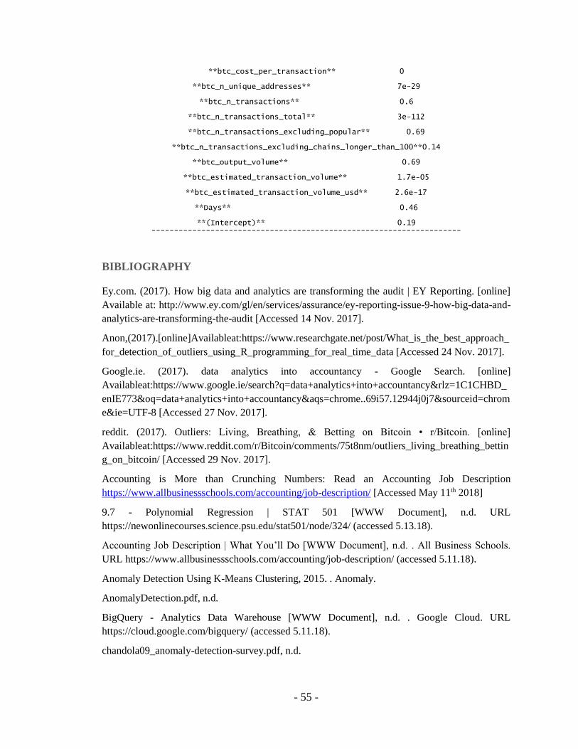
- 55 -
**btc_cost_per_transaction** 0
**btc_n_unique_addresses** 7e-29
**btc_n_transactions** 0.6
**btc_n_transactions_total** 3e-112
**btc_n_transactions_excluding_popular** 0.69
**btc_n_transactions_excluding_chains_longer_than_100**0.14
**btc_output_volume** 0.69
**btc_estimated_transaction_volume** 1.7e-05
**btc_estimated_transaction_volume_usd** 2.6e-17
**Days** 0.46
**(Intercept)** 0.19 --------------------------------------------------------------------
BIBLIOGRAPHY
Ey.com. (2017). How big data and analytics are transforming the audit | EY Reporting. [online]
Available at: http://www.ey.com/gl/en/services/assurance/ey-reporting-issue-9-how-big-data-and-
analytics-are-transforming-the-audit [Accessed 14 Nov. 2017].
Anon,(2017).[online]Availableat:https://www.researchgate.net/post/What_is_the_best_approach_
for_detection_of_outliers_using_R_programming_for_real_time_data [Accessed 24 Nov. 2017].
Google.ie. (2017). data analytics into accountancy - Google Search. [online]
Availableat:https://www.google.ie/search?q=data+analytics+into+accountancy&rlz=1C1CHBD_
enIE773&oq=data+analytics+into+accountancy&aqs=chrome..69i57.12944j0j7&sourceid=chrom
e&ie=UTF-8 [Accessed 27 Nov. 2017].
reddit. (2017). Outliers: Living, Breathing, & Betting on Bitcoin • r/Bitcoin. [online]
Availableat:https://www.reddit.com/r/Bitcoin/comments/75t8nm/outliers_living_breathing_bettin
g_on_bitcoin/ [Accessed 29 Nov. 2017].
Accounting is More than Crunching Numbers: Read an Accounting Job Description
https://www.allbusinessschools.com/accounting/job-description/ [Accessed May 11th 2018]
9.7 - Polynomial Regression | STAT 501 [WWW Document], n.d. URL
https://newonlinecourses.science.psu.edu/stat501/node/324/ (accessed 5.13.18).
Accounting Job Description | What You’ll Do [WWW Document], n.d. . All Business Schools.
URL https://www.allbusinessschools.com/accounting/job-description/ (accessed 5.11.18).
Anomaly Detection Using K-Means Clustering, 2015. . Anomaly.
AnomalyDetection.pdf, n.d.
BigQuery - Analytics Data Warehouse [WWW Document], n.d. . Google Cloud. URL
https://cloud.google.com/bigquery/ (accessed 5.11.18).
chandola09_anomaly-detection-survey.pdf, n.d.

- 56 -
Choudhary, P., n.d. Introduction to Anomaly Detection [WWW Document]. URL
https://www.datascience.com/blog/python-anomaly-detection (accessed 2.26.18).
Cryptocurrency Historical Prices [WWW Document], n.d. URL
https://www.kaggle.com/sudalairajkumar/cryptocurrencypricehistory (accessed 5.13.18).
FAQ How do I interpret a regression model when some variables are log transformed?, n.d. . IDRE
Stats.
Interpreting residual plots to improve your regression | Statwing Documentation [WWW
Document], n.d. URL http://docs.statwing.com/interpreting-residual-plots-to-improve-your-
regression/#hetero-header (accessed 5.13.18).
KDD Process/Overview [WWW Document], n.d. URL
http://www2.cs.uregina.ca/~dbd/cs831/notes/kdd/1_kdd.html (accessed 5.12.18).
Leung, K., Leckie, C., 2005. Unsupervised Anomaly Detection in Network Intrusion Detection
Using Clusters, in: Proceedings of the Twenty-Eighth Australasian Conference on Computer
Science - Volume 38, ACSC ’05. Australian Computer Society, Inc., Darlinghurst, Australia,
Australia, pp. 333–342.
Linear Regression [WWW Document], n.d. URL http://www.stat.yale.edu/Courses/1997-
98/101/linreg.htm (accessed 5.12.18).
Mishra, B.K., Rath, A., Nayak, N.R., Swain, S., 2012. Far efficient K-means clustering algorithm.
ACM Press, p. 106. https://doi.org/10.1145/2345396.2345414
R: What is R? [WWW Document], n.d. URL https://www.r-project.org/about.html (accessed
5.11.18).
Sönmez, F., Zontul, M., Kaynar, O., Tutar, H., 2017. Anomaly Detection Using Data Mining
Methods in IT Systems: A Decision Support Application.
Udacity, n.d. Building the Linear Model - Data Analysis with R.