平成年月日 - mext.go.jp...50 付録1 等パーセンタイル等化法のrプログラム...

49

R スクリプト

50

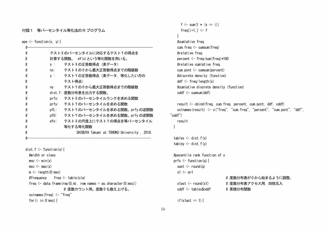
付録１等パーセンタイル等化法のRプログラム

epe <- function(x, y){

#-----------------------------------------------------------------------

# テスト Xのパーセンタイルに対応するテスト Yの得点を

# 計算する関数。 eY(x)という等化関数を用いる。

# x : テスト Xの正答数得点（素データ）

# nx: テスト Xの 0から最大正答数得点までの階級数

# y : テスト Yの正答数得点（素データ，等化したい方の

# テスト得点）

# ny テスト Yの 0から最大正答数得点までの階級数

# dist.f: 度数分布表を出力する関数。

# prfx: テスト Xのパーセンタイルランクを求める関数

# prfy: テスト Yのパーセンタイルを求める関数

# pfL: テスト Yのパーセンタイルを求める関数。prfyの逆関数

# pfU: テスト Yのパーセンタイルを求める関数。prfyの逆関数

# eYx: テスト Xの尺度上にテスト Yの得点を等パーセンタイル

# 等化する等化関数

# SHIBUYA Takumi at TOHOKU University , 2018.

#----------------------------------------------------------------------

dist.f <- function(x){

#width or class

mnc <- min(x)

mxc <- max(x)

m <- length(0:mxc)

#frequancy freq <- table(cla)

freq <- data.frame(rep(0,m), row.names = as.character(0:mxc))

# 度数カウント用。度数 0も数え上げる。

colnames(freq) <- "freq"

for(i in 0:mxc){

f <- sum(1 * (x == i))

freq[i+1,] <- f

}

#cumlative freq.

cum.freq <- cumsum(freq)

#relative freq.

percent <- freq/sum(freq)*100

#relative cumlative freq.

cum.pcnt <- cumsum(percent)

#discrete density (function)

ddf <- freq/length(x)

#cumlative discrete density (function)

cddf <- cumsum(ddf)

result <- cbind(freq, cum.freq, percent, cum.pcnt, ddf, cddf)

colnames(result) <- c("freq", "cum.freq", "percent", "cum.pcnt", "ddf",

"cddf")

result

}

tablex <- dist.f(x)

tabley <- dist.f(y)

#pecentile rank function of x

prfx <- function(q){

xast <- round(q)

x1 <- q+1

# 度数分布表が 0から始まるように調整。

x1ast <- round(x1) # 度数分布表アクセス用，四捨五入

cddf <- tablex$cddf # 累積分布関数

if(x1ast == 1){

51

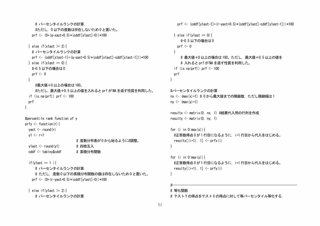
# パーセンタイルランクの計算，

#ただし，0以下の度数は存在しないため 0と置いた。

prf <- (0+(q-xast+0.5)*(cddf[x1ast]-0))*100

} else if(x1ast >= 2){

# パーセンタイルランクの計算

prf <- (cddf[x1ast-1]+(q-xast+0.5)*(cddf[x1ast]-cddf[x1ast-1]))*100

} else if(x1ast == 0){

#-0.5以下の場合は 0

prf <- 0

}

#最大値＋0以上の場合は 100。

#ただし，最大値＋0.5以上の値を入れると prfが NAを返す性質を利用した。

if (is.na(prf)) prf <- 100

prf

}

#percentile rank function of y

prfy <- function(r){

yast <- round(r)

y1 <- r+1

# 度数分布表が 0から始るように#調整。

y1ast <- round(y1) # 四捨五入

cddf <- tabley$cddf # 累積分布関数

if(y1ast == 1 ){

# パーセンタイルランクの計算.

# ただし，度数 0以下の累積分布関数の値は存在しないため 0と置いた。

prf <- (0+(r-yast+0.5)*(cddf[y1ast]-0))*100

} else if(y1ast >= 2){

# パーセンタイルランクの計算

prf <- (cddf[y1ast-1]+(r-yast+0.5)*(cddf[y1ast]-cddf[y1ast-1]))*100

} else if(y1ast == 0){

#-0.5以下の場合は 0

prf <- 0

}

# 最大値＋0以上の場合は 100。ただし，最大値＋0.5以上の値を

# 入れると prfが NAを返す性質を利用した。

if (is.na(prf)) prf <- 100

prf

}

#パーセンタイルランクの計算

nx <- (max(x)+1) # 0から最大値までの階級数，ただし階級幅は 1

ny <- (max(y)+1)

resultx <- matrix(0, nx, 1) #結果代入用の行列を作成

resulty <- matrix(0, ny, 1)

for (i in 0:max(x)){

#正答数得点 0が 1行目になるように，i+1行目から代入をはじめる。

resultx[(i+1), 1] <- prfx(i)

}

for (i in 0:max(y)){

#正答数得点 0が 1行目になるように，i+1行目から代入をはじめる。

resulty[(i+1), 1] <- prfy(i)

}

#------------------------------------------------------------------------

# 等化関数

# テスト Yの得点をテストXの得点に対して等パーセンタイル等化する.

52

# tabley2はこの後のパーセンタイル関数で使用する。

#------------------------------------------------------------------------

tabley2 <- matrix(0, ny, 3)

tabley2[, 1] <- 0:max(y) # 正答数得点

tabley2[, 2] <- tabley [,6] # 累積分布関数

tabley2[, 3] <- resulty # パーセンタイルランク

tabley2 <- as.data.frame(tabley2)

#------------------------------------------------------------------------

# 入力した数値（パーセント）よりも累積パーセントが大きい得点の中で，

# 最も小さい整数値を利用する。

#------------------------------------------------------------------------

pfU <- function(p){

if(p/100 > tabley2$V2[1]){

a <- tabley2[tabley2$V2 >= (p/100),]

yU <- a[1,1]

FyU <- a$V2[1]

b <- tabley2[tabley2$V2 < (p/100),]

FyU1 <- b$V2[yU]

pfU <- (p/100 - FyU1)/(FyU-FyU1) + yU - 0.5

}else if(p/100 == 0){

pfU <- 0

}else{

pfU <- p/100 / tabley2$V2[1] + tabley2$V1[1]-0.5

}

pfU

}

#------------------------------------------------------------------

# こちらは，入力した数値（パーセント）よりも累積パーセントが

# 小さい得点の中で，最も大きい整数値を利用する。

#-------------------------------------------------------------------

pfL <- function(p){

if(p/100 > tabley2$V2[1]){

a <- tabley2[tabley2$V2 >= (p/100),]

yL1 <- a[1,1]

FyL1 <- a$V2[1]

b <- tabley2[tabley2$V2 < (p/100),]

FyL <- b$V2[yL1]

pfL <-(p/100 - FyL)/(FyL1-FyL) + (yL1 - 1) + 0.5

}else if(p/100 == 0){

pfL <- 0

} else {

pfL <- p/100 / tabley2$V2[1] - 1 + 0.5

}

pfL

}

eYx <- matrix(0, nx, 2)

for (i in 1:nx){

eYx[i,1] <- pfU(resultx[i])

eYx[i,2] <- pfL(resultx[i])

}

result <- cbind(resultx, 0:max(x), eYx)

colnames(result) <- c("PR of x", "raw score", "pfU", "pfL")

result

}

#-------------------------------------------------------------------------

# the end of this program

#-------------------------------------------------------------------------

53

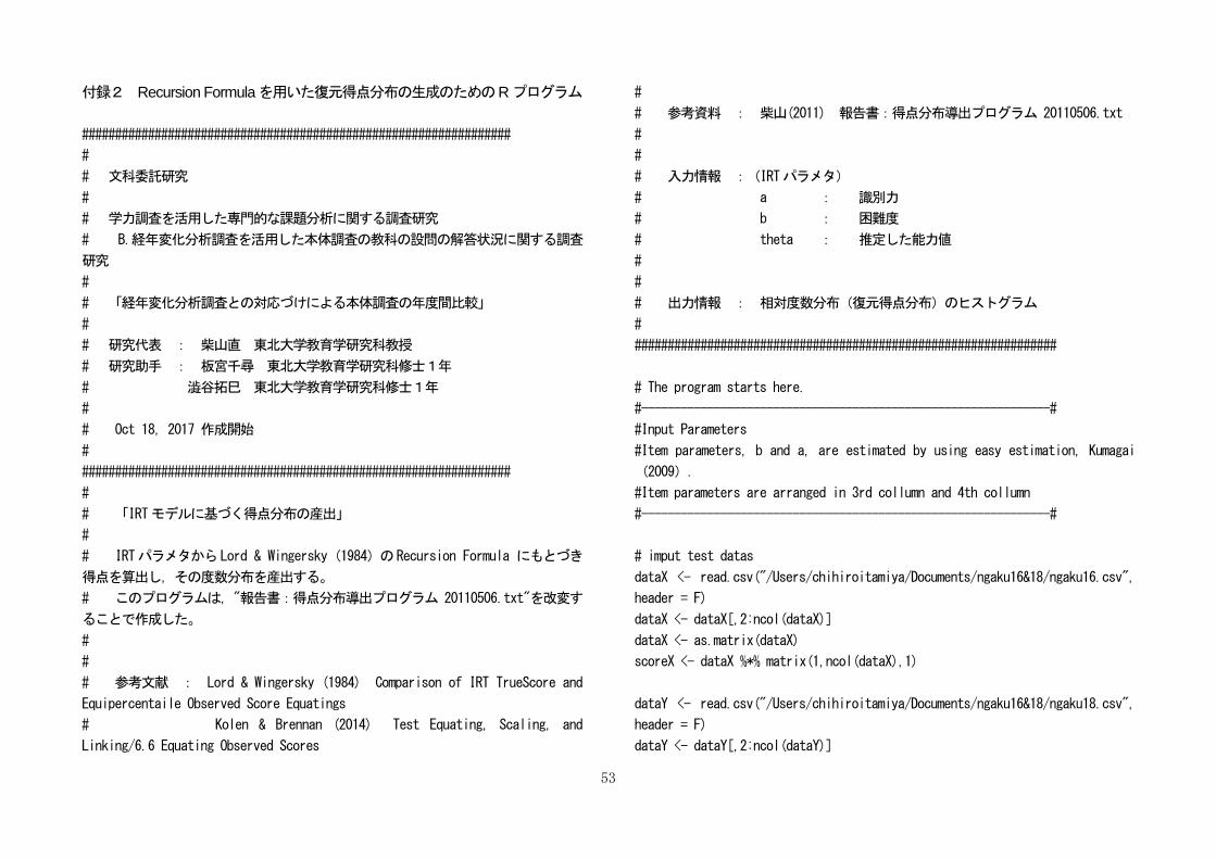
付録２ Recursion Formulaを用いた復元得点分布の生成のためのRプログラム

#################################################################

#

# 文科委託研究

#

# 学力調査を活用した専門的な課題分析に関する調査研究

# B.経年変化分析調査を活用した本体調査の教科の設問の解答状況に関する調査

研究

#

# 「経年変化分析調査との対応づけによる本体調査の年度間比較」

#

# 研究代表：柴山直東北大学教育学研究科教授

# 研究助手：板宮千尋東北大学教育学研究科修士１年

# 澁谷拓巳東北大学教育学研究科修士１年

#

# Oct 18, 2017 作成開始

#

#################################################################

#

# 「IRTモデルに基づく得点分布の産出」

#

# IRTパラメタから Lord & Wingersky（1984）の Recursion Formula にもとづき

得点を算出し，その度数分布を産出する。

# このプログラムは，"報告書：得点分布導出プログラム 20110506.txt"を改変す

ることで作成した。

#

#

# 参考文献： Lord & Wingersky (1984) Comparison of IRT TrueScore and

Equipercentaile Observed Score Equatings

# Kolen & Brennan (2014) Test Equating, Scaling, and

Linking/6.6 Equating Observed Scores

#

# 参考資料：柴山(2011) 報告書：得点分布導出プログラム 20110506.txt

#

#

# 入力情報：（IRTパラメタ）

# a ：識別力

# b ：困難度

# theta ：推定した能力値

#

#

# 出力情報：相対度数分布（復元得点分布）のヒストグラム

#

################################################################

# The program starts here.

#--------------------------------------------------------------#

#Input Parameters

#Item parameters, b and a, are estimated by using easy estimation, Kumagai

（2009）.

#Item parameters are arranged in 3rd collumn and 4th collumn

#--------------------------------------------------------------#

# imput test datas

dataX <- read.csv("/Users/chihiroitamiya/Documents/ngaku16&18/ngaku16.csv",

header = F)

dataX <- dataX[,2:ncol(dataX)]

dataX <- as.matrix(dataX)

scoreX <- dataX %*% matrix(1,ncol(dataX),1)

dataY <- read.csv("/Users/chihiroitamiya/Documents/ngaku16&18/ngaku18.csv",

header = F)

dataY <- dataY[,2:ncol(dataY)]

54

dataY <- as.matrix(dataY)

scoreY <- dataY %*% matrix(1,ncol(dataY),1)

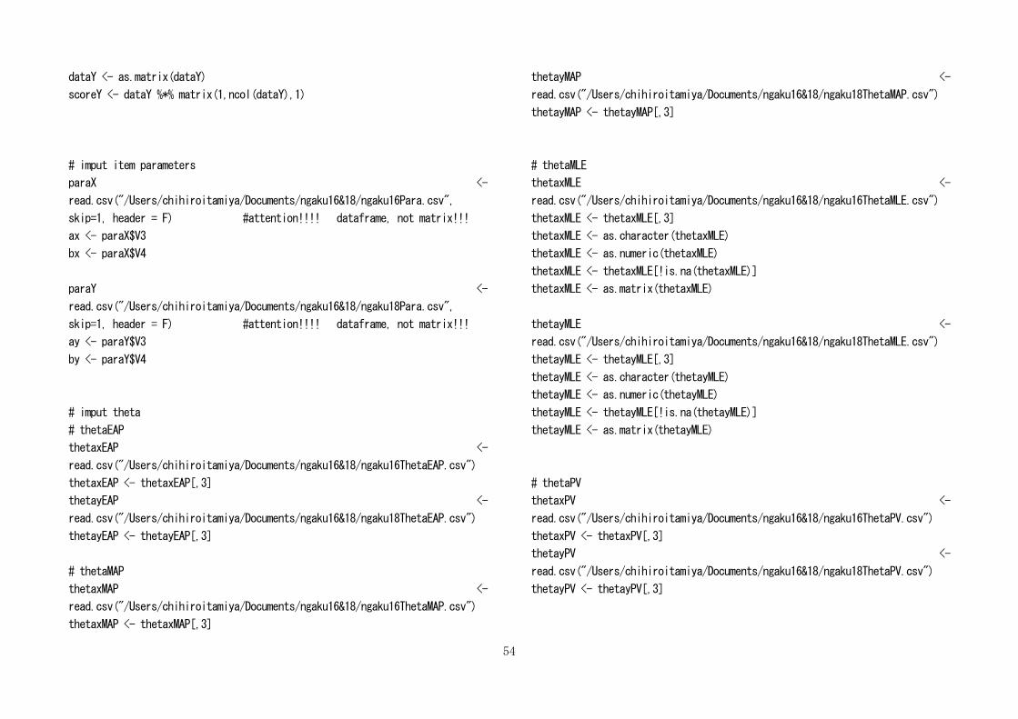
# imput item parameters

paraX <-

read.csv("/Users/chihiroitamiya/Documents/ngaku16&18/ngaku16Para.csv",

skip=1, header = F) #attention!!!! dataframe, not matrix!!!

ax <- paraX$V3

bx <- paraX$V4

paraY <-

read.csv("/Users/chihiroitamiya/Documents/ngaku16&18/ngaku18Para.csv",

skip=1, header = F) #attention!!!! dataframe, not matrix!!!

ay <- paraY$V3

by <- paraY$V4

# imput theta

# thetaEAP

thetaxEAP <-

read.csv("/Users/chihiroitamiya/Documents/ngaku16&18/ngaku16ThetaEAP.csv")

thetaxEAP <- thetaxEAP[,3]

thetayEAP <-

read.csv("/Users/chihiroitamiya/Documents/ngaku16&18/ngaku18ThetaEAP.csv")

thetayEAP <- thetayEAP[,3]

# thetaMAP

thetaxMAP <-

read.csv("/Users/chihiroitamiya/Documents/ngaku16&18/ngaku16ThetaMAP.csv")

thetaxMAP <- thetaxMAP[,3]

thetayMAP <-

read.csv("/Users/chihiroitamiya/Documents/ngaku16&18/ngaku18ThetaMAP.csv")

thetayMAP <- thetayMAP[,3]

# thetaMLE

thetaxMLE <-

read.csv("/Users/chihiroitamiya/Documents/ngaku16&18/ngaku16ThetaMLE.csv")

thetaxMLE <- thetaxMLE[,3]

thetaxMLE <- as.character(thetaxMLE)

thetaxMLE <- as.numeric(thetaxMLE)

thetaxMLE <- thetaxMLE[!is.na(thetaxMLE)]

thetaxMLE <- as.matrix(thetaxMLE)

thetayMLE <-

read.csv("/Users/chihiroitamiya/Documents/ngaku16&18/ngaku18ThetaMLE.csv")

thetayMLE <- thetayMLE[,3]

thetayMLE <- as.character(thetayMLE)

thetayMLE <- as.numeric(thetayMLE)

thetayMLE <- thetayMLE[!is.na(thetayMLE)]

thetayMLE <- as.matrix(thetayMLE)

# thetaPV

thetaxPV <-

read.csv("/Users/chihiroitamiya/Documents/ngaku16&18/ngaku16ThetaPV.csv")

thetaxPV <- thetaxPV[,3]

thetayPV <-

read.csv("/Users/chihiroitamiya/Documents/ngaku16&18/ngaku18ThetaPV.csv")

thetayPV <- thetayPV[,3]

55

# 復元得点分布(IRT observed score distribution)のヒストグラム,累積度数分布を

描画

score.dist <- function(theta,ax,bx,cumulative=T,max.x=max(score, na.rm =

TRUE),

col="blue",lty=1,type="l",name="score distribution"){

#--------------------------------------------------------------#

# This function generates distribution of IRT observed scores

# on 2-parameter logistic model.

#

# m : number of items

# n : number of subjects

# rn : number of normal random numbers

# theta : ability

# a : item discriminating powers

# b : item difficulties

# name : main title of the histogram

# col : color of the histogram

# lty : line type

# type : plot type

# cumulative : draw a cumulative distribution

#

# This function developed by C. ITAMIYA and T. SHIBUYA., October 2017.

# The Original syntax is written by T. SHIBAYAMA.

#

#

#--------------------------------------------------------------#

# Number of Items and Subjects

#--------------------------------------------------------------#

mx <- length(ax) #n of items

mx1 <- mx+1

thetax <- theta

n <- length(thetax) #n of subjects

#--------------------------------------------------------------#

# Distribution of Ability

#--------------------------------------------------------------#

i <- sort.list(thetax)

thetax <- thetax[i]

i <- matrix(1:n,1,n)

#--------------------------------------------------------------#

# Conditional Probabilities of Test Scores

#--------------------------------------------------------------#

probability <- function(trait,a,b){

#--------------------------------------------------------------#

# This function generates conditional probability

# for a fixed ability on 2-parameter logistic model.

#

# The original Fortran77 program was

# developed by Inoue,S. , December 1990.

# extended by Shibayama,T., January 1991.

# translated into R by Shibayama,T. September 2008.

#


# trait : ability



# prb : conditional probability for a fixed ability

# ptheta : P(theta)

# qtheta : Q(theta)=1-P(theta)

#--------------------------------------------------------------#

m <- length(a)

m1 <- m+1

ptheta <- matrix(0,m,1)

qtheta <- matrix(0,m,1)

56

prb <- matrix(0,m1,1)

#

ptheta<- 1/(1+exp(-1.7*a*(trait-b)))

qtheta<- 1-ptheta

#

prb[1] <- qtheta[1]

prb[2] <- ptheta[1]

#

for(j in 2:m){

l <- j -1

j1 <- j+1

l1 <- l+1

prb[j1] <- prb[l1]*ptheta[j]

for(i in l:1){

k <- i -1

i1 <- i+1

k1 <- k+1

prb[i1]<-prb[k1]*ptheta[j]+prb[i1]*qtheta[j]

}

prb[1] <- prb[1]*qtheta[j]

}

#

probability <- prb

#

}

#cat("¥nrecursion formula 実行中")

prbtestscore<-matrix(0,n,mx1)

for(i in 1:n){

#spbar(i/n)

prbtestscore[i,]<- t(probability(thetax[i],ax,bx))

}

#--------------------------------------------------------------#

# Marginal Probabilities of Test Score

#--------------------------------------------------------------#

xfreq <- t(prbtestscore) %*% matrix(1,n,1)

xfreq <-cbind(matrix(0:mx,mx1,1),xfreq)

temp <- round(xfreq[,2]) #度数の小数点以下を四捨五

入する

sum(temp)

#temp2 <- temp/sum(temp)

score <- rep(xfreq[,1],temp) #度数分布表をベクトルに展

開する

mx <- max(score)

if(cumulative <- cumulative){

cumulative <- cumsum(xfreq[,2]/n)

cumulative <- cbind(matrix(0:mx,mx1,1),cumulative)

quartz()

#win.graph()

plot(cumulative,col=col,lty=lty,type=type,xlab="score",ylab="relative

cumulative frequency",main=name,

xlim=c(0,max.x),ylim=c(0,1),cex=0.5,cex.main=1.5,cex.lab=1.5,cex.axis=1.3)

}else{

quartz()

#win.graph()

hist(score,col=col,xlab="score",ylab="relative

frequency",main=name,freq=FALSE,ylim=c(0,0.15),

breaks=seq(-0.5,(mx+0.5),1),cex.main=1.5,cex.axis=1.3,cex.lab=1.3)

#相対度数分布のヒストグラムを近似的に描画する

57

#n <- length(score)

}

}

# 度数・相対度数・累積度数・累積相対度数をデータフレームで出力

# 得点分布を度数に基づきベクトルに展開

dist.data <- function(theta,a,b,frequency=T){

#--------------------------------------------------------------#

# This function generates numeric data of frequency distribution

# IRT observed scores on 2-parameter logistic model.

#


# n : number of subjects

# rn : number of normal random numbers

# theta : ability



# frequency : write a table of frequency distribution

#

# This function developed by C. ITAMIYA and T. SHIBUYA., October 2017.


#

#--------------------------------------------------------------#

a <- as.matrix(a) #項目パラメタを行列形式

にする

b <- as.matrix(b)

theta <- as.matrix(theta)

#--------------------------------------------------------------#


#--------------------------------------------------------------#

m <- nrow(a) #n of items

m1 <- m+1

n <- nrow(theta) #n of subjects (thetaに推定した能力値を代入する場合)

#--------------------------------------------------------------#


#--------------------------------------------------------------#

i <- sort.list(theta) #thetaを昇順に並べる

theta <- theta[i]


#--------------------------------------------------------------#

# Conditional Probabilities of Test Scores

#--------------------------------------------------------------#

probability <- function(trait,a,b){

#--------------------------------------------------------------#

# This function generates conditional probability

# for a fixed ability on 2-parameter logistic model.

#

# The original Fortran77 program was

# developed by Inoue,S. , December 1990.

# extended by Shibayama,T., January 1991.

# translated into R by Shibayama,T. September 2008.

#

58


# trait : ability



# prb : conditional probability for a fixed ability

# ptheta : P(theta)

# qtheta : Q(theta)=1-P(theta)

#--------------------------------------------------------------#

m <- nrow(a)

m1 <- m+1

ptheta <- matrix(0,m,1)

qtheta <- matrix(0,m,1)

prb <- matrix(0,m1,1)

#


qtheta<- 1-ptheta

#

prb[1] <- qtheta[1]

prb[2] <- ptheta[1]

#

for(j in 2:m){

l <- j -1

j1 <- j+1

l1 <- l+1

prb[j1] <- prb[l1]*ptheta[j]

for(i in l:1){

k <- i -1

i1 <- i+1

k1 <- k+1

prb[i1]<-prb[k1]*ptheta[j]+prb[i1]*qtheta[j]

}

prb[1] <- prb[1]*qtheta[j]

}

#

probability <- prb

#

}

prbtestscore<-matrix(0,n,m1)

for(i in 1:n){

prbtestscore[i,]<- t(probability(theta[i],a,b))

}

#--------------------------------------------------------------#

# Marginal Probabilities of Test Score

#--------------------------------------------------------------#

freq <- colSums(prbtestscore)

freq <- cbind(matrix(0:m,m1,1),freq) #[得点｜度数分布]

if(frequency <- frequency){

#temp <- round(freq[,2]) #度数の小数

点以下を四捨五入する

#score <- rep(freq[,1],temp) #度数分布表をベクト

ルに展開する

#mx <- max(score)

#mean.observed <- mean(score)

#sd.observed <- sd(score)

#scoredata <- data.frame(平均=mean.observed,標準偏差=sd.observed)

#print(scoredata)

59

dist <- freq[,2]/sum(freq[,2]) #相対度数分布

cumulative <- cumsum(freq[,2]) #累積度数分布

cum.relative <- cumulative/n #累積相対度数分布

distribution <- data.frame(得点=freq[,1],度数=(freq[,2]),相対度数=dist,

累積度数=cumulative,累積相対度数=cum.relative)

return(distribution)

}else{

temp <- round(freq[,2]) #度数の小数点以下を四捨五入する

score <- rep(freq[,1],temp) #度数分布表をベクトルに展開する

return(score)

}

}

# true score distribution・raw score distributionについて（参考）

# true score distributionのヒストグラム

#----------------------------------------------------------------#

truescore.hist <- function(theta,a,b,name="test",color="cyan"){

#--------------------------------------------------------------#

a <- as.matrix(a) #項目パラメタを行列形式

にする

b <- as.matrix(b)



m <- length(a) #n of items

m1 <- m+1

n <- length(theta) #n of subjects


i <- sort.list(theta)

theta <- theta[i]


# Comditional Probabilities of True Scores

#------------------------------------------------------------#

truescore<-function(trait,a,b){

#----------------------------------------------------------#

# This function generates true scores

# 2-parameter logistic model.

#

## m : number of items

# trait : ability



# ptheta : P(theta)

# tscore : true scores

#

m <- nrow(a)

m1 <- m+1

#ptheta<- matrix(0,m,1)

#


#

truescore <- sum(ptheta)

#

}

#------------------------------------------------------------#

tscore <- matrix(0,n,1)

for(i in 1:n){

tscore[i,] <- t(truescore(theta[i],a,b))

}

60

quartz()

hist(tscore,freq=FALSE,ylim=c(0,0.20),breaks=seq(-0.5,(mx+0.5),1),

xlab="score",col=color,main=name,cex.main=1.5,cex.lab=1.3,cex.axis=1.3)

}

#----------------------------------------------------------------#

# true score の累積度数分布

#----------------------------------------------------------------#

cum.truescore <- function(theta,a,b){

#--------------------------------------------------------------#


#--------------------------------------------------------------#

mx <- length(a) #n of items

mx1 <- mx+1

n <- length(theta) #n of subjects

#--------------------------------------------------------------#


#--------------------------------------------------------------#

i <- sort.list(theta)

theta <- theta[i]


#--------------------------------------------------------------#

truescore<-function(trait,a,b){

#------------------------------------------------------------#

# This function generates true scores

# 2-parameter logistic model.

#

## m : number of items

# trait : ability



# ptheta : P(theta)

# tscore : true scores

#

m <- nrow(a)

m1 <- m+1

#ptheta<- matrix(0,m,1)

#


#

truescore <- sum(ptheta)

#

}

#

#------------------------------------------------------#

# True Scores

#------------------------------------------------------#

tscore <- matrix(0,n,1)

for(i in 1:n){

tscore[i,] <- t(truescore(theta[i],a,b))

}

tscore <- round(tscore)

mean.tscore <- mean(tscore)

sd.tscore <- sd(tscore)

scoredata <- data.frame(平均=mean.tscore,標準偏差=sd.tscore)

print(scoredata)

61

dist.f <- function(w){

cla <- w

mnc <- min(cla)

mxc <- max(cla)

cla <- factor(cla,levels=mnc:mxc)

freq <- table(cla)




ddf <- freq/length(w)

cddf <- cumsum(ddf)

names(freq) <- paste(mnc:mxc)

return(cbind(freq,cum.freq,percent,cum.pcnt,ddf,cddf))

}

dist.f(tscore)

cum.freq <- dist.f(tscore)

cum.freq <- cbind(c(0:(length(cum.freq[,2])-1)),cum.freq[,2]/n)

plot(cum.freq,type="l",col="black",xlab="score",ylab="relative cumulative

frequency",

xlim=c(0,25),ylim=c(0,1),lty=4)

}

#----------------------------------------------------------------#

# raw score distribution（素得点分布）のヒストグラム

#----------------------------------------------------------------#

# FormX

quartz()

hist(scoreX,freq=FALSE,ylim=c(0,0.15),breaks=seq(-

0.5,(25+0.5),1),col="#A9A9A9",

main="raw score distribution of FormX",cex.main=1.5)

# FormY

quartz()

hist(scoreY,freq=FALSE,ylim=c(0,0.15),breaks=seq(-

0.5,(25+0.5),1),col="gray",

xlab="score",main="raw score distribution of FormY",cex.main=1.5)

#----------------------------------------------------------------#

# raw score の累積度数分布

#----------------------------------------------------------------#

rawcum.hist <- function(score,color="black",max.x=max(score, na.rm =

TRUE),LTY=1,

name="cumulative frequency distribution",sname=""){

dist.f <- function(w){

cla <- w

mnc <- min(cla, na.rm = TRUE)

mxc <- max(cla, na.rm = TRUE)

cla <- factor(cla,levels=mnc:mxc,exclude = NA)

freq <- table(cla)




ddf <- freq/length(w)

cddf <- cumsum(ddf)

names(freq) <- paste(mnc:mxc)

return(cbind(freq,cum.freq,percent,cum.pcnt,ddf,cddf))

}

mean.raw <- mean(score)

sd.raw <- sd(score)

scoredata <- data.frame(平均=mean.raw,標準偏差=sd.raw)

print(scoredata)

62

dist.f(score)

cum.freq <- dist.f(score)

cum.freq <- cbind(c(0:(length(cum.freq[,2])-1)),cum.freq[,4]/100)

plot(cum.freq,type="l",col=color,xlab="score",ylab="relative cumulative

frequency",

xlim=c(0,max.x),ylim=c(0,1),lty=LTY,main=name,sub=sname)

}

#----------------------------------------------------------------#

63

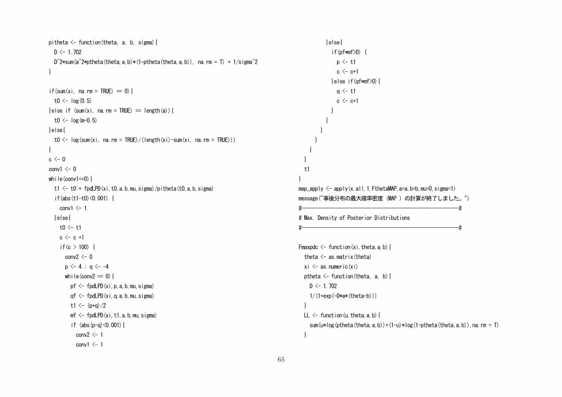
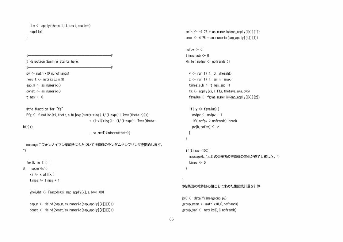
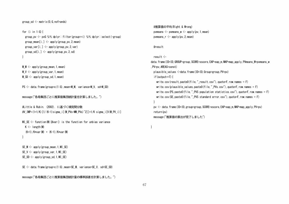
付録３フォンノイマン棄却法を用いた推算値算出のためのRプログラム

plausible <- function(xall, param, gh, nofrands=10,

file="default",output=FALSE,IDc=1,Gc=2,ITEMc=3){

library(dplyr)

#--------------------------------------------#

# This function edited by D. EJIRI and T. SHIBUYA.


# Oct. 10 2017 Debug by Ejiri. -> fg value,

# Oct. 22 2017 Debug by Shibuya.

# Nov. 10 2017 Edit by Ejiri to output result for CSV file.

# Feb. 21 2018 Modified by Shibuya to estimate MAP and set MAP estimator as the

Max density for the Rejection sampling.

# MAP estimate iterration algorithm is basd on Newton Raphthon and

bisection method.

# Apr. 3 2018 Modified by Shibuya to use apply familly and acceleration

estimating MAP and EAP.

# Apr. 5 2018 Edited by Shibuya. Add function to estimate standard error of

imputation.

#--------------------------------------------#

#----

#xall:dichotomously item response data.It has ID in first column, group number in

second column.

#para:item parameter data. It has discrimination parameter in first column,

difficulty parameter in second column.

#nofrands:the number of plausible values

#gh: Nodes and weights for the Gauss-Hermite formula, csv file.It has nodes in

second column and weihts in third column.

#----

message("推算値の計算を始めます。")

message("データチェック")

ID <- xall[,IDc]

if(Gc == 0){

group <- rep(1, nrow(xall))

G <- 1

x.all <- xall[,ITEMc:ncol(xall)]

}else{

group <- xall[,Gc]

G <- max(as.numeric(group))

x.all <- xall[,ITEMc:ncol(xall)]

}

#remove a=0 item parameter and response column

message("識別力が0の項目を削除します。")

a <- param[,1]

x.all <- x.all[, a != 0]

message(sum((a == 0)*1),"個の項目が削除されました。")

#set item parameter data

param <- param[param[,1] != 0, ]

a <- param[,1]

b <- param[,2]

# Number of Subjects"

n <- nrow(xall)

# number of items

m <-length(a)

xscore <- rowSums(x.all,na.rm=T)

message("IDと項目反応データ，項目母数を確認しました。")

message("母集団",G)

message(",受検者",n,"人，項目数",m,"個でした")

64

### Nodes and weights for the 5-point Gauss-Hermite formula ####

#

# Integrate of f(x) * exp(-x^2) = Sum of f(x) * weight

#

# ex. Integrate of exp(-x^2) = sqrt(pi) = 1.772454

# Sum of weights = 1.772454

#---------------------------------------------------------------

# Xm <- seq(-4,4,length.out=15);Wm <- dnorm(Xm,0,1);Wm <- Wm/sum(Wm)

npoint <- nrow(gh)

xnodes <- gh$xi*sqrt(2)

weight <- gh$wi/sqrt(pi) #caribration

message(npoint,"分点のガウス・エルミート求積法のノードとウェイトを読み込みました。

")

#--------------------------------------------#

#EAP parameter

#--------------------------------------------#

FthetaEAP <- function(xi,theta,w,a,b){

theta <- as.matrix(theta,byrow=T)

xi <- as.numeric(xi)

ptheta <- function(theta, a, b){

D <- 1.702

1/(1+exp(-D*a*(theta-b)))

}

LL <- function(u,theta,a,b){

sum(u*log(ptheta(theta,a,b))+(1-u)*log(1-ptheta(theta,a,b)),na.rm = T)

}

LLm <- apply(theta,1,LL,u=xi,a=a,b=b)

Lm <- exp(LLm)

Gm <- Lm*w/sum(Lm*w,na.rm = T)

const <- sum(Lm*w,na.rm = T)

return(list(sum(theta*Gm,na.rm = T),const))

}

eap_apply <- apply(x.all,1,FthetaEAP,a=a,b=b,theta=xnodes,w=weight)

message("EAPと周辺分布の計算が終了しました。")

#Eatimate MAP

FthetaMAP <- function(xi,a,b,mu,sigma){

#-----

#引数について

#xall: 項目反応データ

#a&b: 母数ファイル。aが識別力，bが困難度

#mu&sigma: 事前分布の平均と標準偏差

#-----

#P(theta) in two-parameter logisticmodel


D <- 1.702


}

#the first partial derivative

fpdLPD <- function(xi, theta, a, b, mu, sigma){

D <- 1.702

D*sum(a*(xi - ptheta(theta,a,b)), na.rm = T) - (theta-mu)/sigma^2

}

#posterior information

65

pitheta <- function(theta, a, b, sigma){

D <- 1.702

D^2*sum(a^2*ptheta(theta,a,b)*(1-ptheta(theta,a,b)), na.rm = T) + 1/sigma^2

}

if(sum(xi, na.rm = TRUE) == 0){

t0 <- log(0.5)

}else if (sum(xi, na.rm = TRUE) == length(a)){

t0 <- log(m-0.5)

}else{

t0 <- log(sum(xi, na.rm = TRUE)/(length(xi)-sum(xi, na.rm = TRUE)))

}

c <- 0

conv1 <- 0

while(conv1==0){

t1 <- t0 + fpdLPD(xi,t0,a,b,mu,sigma)/pitheta(t0,a,b,sigma)

if(abs(t1-t0)<0.001) {

conv1 <- 1

}else{

t0 <- t1

c <- c +1

if(c > 100) {

conv2 <- 0

p <- 4 ; q <- -4

while(conv2 == 0){

pf <- fpdLPD(xi,p,a,b,mu,sigma)

qf <- fpdLPD(xi,q,a,b,mu,sigma)

t1 <- (p+q)/2

mf <- fpdLPD(xi,t1,a,b,mu,sigma)

if (abs(p-q)<0.001){

conv2 <- 1

conv1 <- 1

}else{

if(pf*mf>0) {

p <- t1

c <- c+1

}else if(qf*mf>0){

q <- t1

c <- c+1

}

}

}

}

}

}

t1

}

map_apply <- apply(x.all,1,FthetaMAP,a=a,b=b,mu=0,sigma=1)

message("事後分布の最大確率密度（MAP ）の計算が終了しました。")

#----------------------------------------------------------#

# Max. Density of Posterior Distributions

#----------------------------------------------------------#

Fmaxpdc <- function(xi,theta,a,b){


xi <- as.numeric(xi)


D <- 1.702


}

LL <- function(u,theta,a,b){

sum(u*log(ptheta(theta,a,b))+(1-u)*log(1-ptheta(theta,a,b)),na.rm = T)

}

66

LLm <- apply(theta,1,LL,u=xi,a=a,b=b)

exp(LLm)

}

#--------------------------------------------------#

# Rejection Samling starts here.

#--------------------------------------------------#

pv <- matrix(0,n,nofrands)

result <- matrix(0,n,3)

eap_m <- as.numeric()

const <- as.numeric()

times <- 0

#the function for "fg"

Ffg <- function(xi,theta,a,b){exp(sum(xi*log( 1/(1+exp(-1.7*a*(theta-b))))

+ (1-xi)*log(1- (1/(1+exp(-1.7*a*(theta-

b)))))

, na.rm=T))*dnorm(theta)}

message("フォンノイマン棄却法にもとづいて推算値のランダムサンプリングを開始します。

")

for(k in 1:n){

# spbar(k/n)

xi <- x.all[k,]

times <- times + 1

yheight <- Fmaxpdc(xi,map_apply[k],a,b)*1.001

eap_m <- rbind(eap_m,as.numeric(eap_apply[[k]][1]))

const <- rbind(const,as.numeric(eap_apply[[k]][2]))

zmin <- -4.75 + as.numeric(eap_apply[[k]][1])

zmax <- 4.75 + as.numeric(eap_apply[[k]][1])

nofpv <- 0

times_sub <- 0

while( nofpv <= nofrands ){

y <- runif( 1, 0, yheight)

z <- runif( 1, zmin, zmax)

times_sub <- times_sub +1

fg <- apply(xi,1,Ffg,theta=z,a=a,b=b)

fgvalue <- fg/as.numeric(eap_apply[[k]][2])

if( y <= fgvalue){

nofpv <- nofpv + 1

if( nofpv > nofrands) break

pv[k,nofpv] <- z

}

}

if(times==100){

message(k,"人目の受検者の推算値の発生が終了しました。")

times <- 0

}

}

#各集団の推算値の組ごとに求めた集団統計量を計算

pvG <- data.frame(group,pv)

group_mean <- matrix(0,G,nofrands)

group_var <- matrix(0,G,nofrands)

67

group_sd <- matrix(0,G,nofrands)

for (i in 1:G){

group_pv <- pvG %>% dplyr::filter(group==i) %>% dplyr::select(-group)

group_mean[i,] <- apply(group_pv,2,mean)

group_var[i,] <- apply(group_pv,2,var)

group_sd[i,] <- apply(group_pv,2,sd)

}

M_M <- apply(group_mean,1,mean)

M_V <- apply(group_var,1,mean)

M_SD <- apply(group_sd,1,mean)

PS <- data.frame(group=c(1:G),mean=M_M, variance=M_V, sd=M_SD)

message("各母集団ごとに推算値集団統計量を計算しました。")

#Little & Rubin. (2002). に基づく補完間分散

#V_IMP=(1+1/K)[1/(K-1)sigma_i[(M_PVs-MM_PVs)^2]]+1/K sigma_i[V(M_PV_i)]

MI_SE <- function(M){#var() is the function for unbias variance

K <- length(M)

(K+1)/K*var(M) + (K-1)/K*var(M)

}

SE_M <- apply(group_mean,1,MI_SE)

SE_V <- apply(group_var,1,MI_SE)

SE_SD <- apply(group_sd,1,MI_SE)

SE <- data.frame(group=c(1:G),mean=SE_M, variance=SE_V, sd=SE_SD)

message("各母集団ごとに推算値集団統計量の標準誤差を計算しました。")

#推算値の平均(Right & Wrong)

pvmeans <- pvmeans_w <- apply(pv,1,mean)

pvmeans_r <- apply(pv,2,mean)

#result

result <-

data.frame(ID=ID,GROUP=group,SCORE=xscore,EAP=eap_m,MAP=map_apply,PVmeans_W=pvmeans_w

,PV=pv,AREAS=const)

plausible_values <-data.frame(ID=ID,Group=group,PV=pv)

if(output==T){

write.csv(result,paste0(file,"_result.csv"),quote=F,row.names = F)

write.csv(plausible_values,paste0(file,"_PVs.csv"),quote=F,row.names = F)

write.csv(PS,paste0(file,"_PVS population statistics.csv"),quote=F,row.names = F)

write.csv(SE,paste0(file,"_PVS standard error.csv"),quote=F,row.names = F)

}

pv <- data.frame(ID=ID,group=group,SCORE=xscore,EAP=eap_m,MAP=map_apply,PV=pv)

return(pv)

message("推算値の算出が完了しました")

}

平成 年 月 日 - mext.go.jp...50 付録1 等パーセンタイル等化法のrプログラム...

Documents

平成年月日 - mext.go.jp...50 付録1 等パーセンタイル等化法のrプログラム...