E CPE

- 29 -

E GOVERNMENTD NG IN THE U.S.:

acts and Theoriesby Edward M. Gramlich

CONTENTS

Introduction

Growth Theories

, 31

Government Growth and Borcherding's ResidualHypothesis 33Government Growth and Baumol's Productivity DisparityHypothesis . . . . . . . . . . . . . . . . .. 39

Levet Theor-es . . . . . . . . . . . . . . . . .. 44The Voting Distortion Hypothesis of Borcherding-Bush-Spann 44The Redistribution Hypothesis of Peltzman 53The Public Wage Growth Hypothesis of Courant-Gramlich-Rubinfeld 56

Summary and Implications 60

Tables

eferences

63

70

- 31 -

1:0

The United States has neither the highest nor the

most rapidly growing share of national output de­

voted to public spending of the major western

industrial countries. Rut it does have by far the

most discussion wi thin i ts economic profession of

the question of excessive government spending.

United States economists have been responsible for

several different models of excessive government

spending. They have devised Consti tutional amend­

ments to limit spending, and they have been in the

forefront of political campaigns on the issue. In

America the question of the size and growth of

governrnent has been as rnuch one of the deve10prnent

of econornic thought in the field of applied public

finance as it has of the basic facts.

In this paper I try to review both the facts and

the theories coming from the American experience.

The facts are obviously particular to the United

States and only relevant to other countries to the

extent that similar things are happening there for

similar reasons • The theories are obviously not

particular to the United States , but of more gen­

eral interest. The paper will therefore focus more

attention on them.

Five theories will be summarized, two regarding

the growth of government spending over time and

three regarding reasons why the leve1 of govern­

ment spending may be excessive. The five are:

Growth theories

l) Borcherding's (1977) positive residual hypoth­

esis:

,i

I I

i

- 32 -

2) Baumol ' s (1967) productivity disparity hypoth-

esis;

Level"theories

l) Borcherding-Bush-Spann's (1977) voting distor­

tion hypothesi s i

2) Peltzman1s (1980) redistribution hypothesisi

3) Courant-Gramlich-Rubinfeld I s (1979) public wage

hypothesis.

For each I will try to provide informal tests of

the hypothesis using either macro statistics or

the results of voter surveys taken after same

recent statewide tax limitation votes. These tests

will basically be aimed at trying to determine

whether there is or is not strong evidence that

government spending growth rates or levels are

excessive in the United States today. At the

outset, however, I must warn that the tests are

not able to confirm or refute every aspeet of

every theory, and sometimes not even the most

important aspects of the theories. Moreover , the

business of creating theories to explain govern­

ment growth is booming so mueh now that even these

theories do not exhaust the set, so other interest­

ing views will be ignored. Finally, most of the

facts used in the paper will foeus on aetual gov­

ernrnent spending, ignoring the new and interesting

area of governrnent regulation of the private

sector -- an area that is now beginning to spawn

its own theories.

- 33 -

GoverDlleDt Grovth and Borcberding· s Re idual

Bypot:hesis

The rnain idea behind Borcherding's residual hypoth­

esis is that governrnent growth is excessive if i t

cannot be explained. He tries to predict govern­

ment growth by applying elasticities estimated

from cross-sectional data to growth rates of impor­

tant independent variables and finds large posi­

tive residuals . These residuals growth unac­

counted for by rnovernents in the independent vari­

ables -- suggest the existence of same mysterious,

or at least nonquantifiable, force pushing up gov­

ernment budgets and tax rates.

There are serious problems in interpreting such a

test because not all nonquantifiable rnovements

imply that government growth is excessive. If, for

example, government spending was too low at the

start of some period, rapid and unexplained growth

would imply only that the initial disequilibrium

was being corrected. Or, tastes for public expendi­

tures might shift over some interval, resulting in

apparently unexplainable growth. But even though

there are such problems of interpretation, i t is

still useful to go through the Borcherding exer­

cise as a way of organizing the facts of the U.S.

experience.

The actual residual test can be developed by solv­

ing a three equation model. The first is a stand­

ard public goods demand function, written as

X,1.

c cA y,l p,2

1. 1.(l )

- 34 -

where X. refers to the utility services conferredl

by a unit of public spending, A is a constant, Y.l

is income, and P. is the tax price of a unit of1

these services, with the i subscript referring to-

the IIdecisive ll voter in the community. cl(>O)

refers to the income elasticity of public goods

demand and c2«0) the relative price elasticity.

In the straightforward median voter theory of

Hotelling (1929), Bowen (1943), and Downs (1957),

the ith citizen is the median voter, but given

various kinds of imperfections and gaps in infor­

mation, the model can be generalized to make i

refer to the particular voter who, upon changing

his or her vote, can alter the political outcome.

Utility services are then related to public goods

purchases by the crowding expression of Borcherd­

ing-Deacon (1972) and Bergstrom-Goodman (1973):

X.l

aG/N l, ( 2 )

where N is community population and G is the real

purchases of public goods in the community. When

al = O, the good or service in question is a Samu­

elsonian (1954) public good and increments to po-

pulation do not lower the utility services receiv­

ed by the i th voter. When al = l, the good is

crowdable in that added consumers do lower util­

ity proportionately, even though the good may

still be supplied through the public sector (an

example is public schooling) .

. The tax price for a unit of public services can be

expressed as the product of three components, the

gross price of a unit of public output, the tax

share of the decisive voter, and the inverse of

the crowding function:

a(p)(Y.jY)(N 1),

1

- 35 -

(3 )

where P is the gross relative price of a unit of

public services and Y is the communi ty tax base.

The second term shows how much of this relative

price will be paid by the decisive voter, and the

third term adjusts for crowding. Whenever al > O,

the cost to the decisive voter of a unit of public

services varies directly with community population

(the more people in the community, the more public

goods one has to buy to gain a unit of utility) .

Inserting (2) and (3) into (1), taking logs, di f­

ferentiating, and using the approximation that

d~nY. = d~nY - d~nN yields as the general growth1

equation for public expenditures

d1nG = c 1 d1nY + c 2d1np + (al (l+c 2 ) - c l - c2)d~nN

(4)

Other things equal, governrnent spending will rise

with income but will increase less the more public

seetor relative prices rise. Borcherding's point,

very simply, is that the equation has not worked:

that actual growth rates on the left side have ex­

eeeded predicted growth rates on the right side.

Before actually exarnining these residuals, one

aspect of equation (4) should be emphasized. Most

studies of public goods demands in the United

States find ineome elasticities (el) that are less

than one, and price e1asticities (c 2 ) that are

negative. These findings are characteristic for

every one of eleven comrnonly eited recent empir­

ieal studies, listed in Table l. If such is the

case, and if O < al < l as required by the theory,

- 36 -

the predieted growth rate of government spending

may weIl be less than the growth rate of GNP.

Henee it may be possible to find eases where Bor­

eherding's residuals are positive that is, gov­

ernment spending is growing more rapidly than

would be predicted by an equation such as (4), but

the share o f government in real GNP is ei ther

stable or declining. In broad outline, this ap-

pears to be happenJ.ng in the United States i at

least for certain types of expenditures. l

To make the actual comparisons I foeus on three

types of government expenditures:

a) exhaustive purehases for national defense

b) other exhaustive purchases

c) transfer payments

The comparisons aggregate national, state, and

loeal government spending for the speeified catego­

ries, and thus obviate the need to worry about

rapidly growing intergovernmental grants. I will

also ignore subsidies of governmental enterprises,

which are small and best thought of as negative

indireet taxes, and interest payments on -governmen­

tal debt, which can be explained by a straightfor­

ward relationship with interest rates.

Table 2 gives the residual comparisons for the

three types of expenditures for the last five

decades . National defense is perhaps not a good

plaee to begin because the growth comparisons are

l Note, however, that this staternent refers onlyto the share of government spending in real GNP.If P is rising and c 2 is less than one in absolutevalue, the money share of government spending (GP)could be increasing. Qates' paper in this volurnefoeuses on that ratio.

- 37 -

seriously distorted first by World War II, then by

the Cold War buildup, and finally by the Vietnam

War expenditures in the late sixties. Moreover, to

my knowledge nobody has provided estimates of

income and price elasticities for national de­

fense. Yet because these purchases are so impor­

tant in shaping overall government spending levels

in America, these comparisons are given in the top

panel of the Table. For these comparisons c l and

c 2 are taken at the mean values shown in Table l,

and al is assumed to equal zero since national

defense expenditures are the classic example of a

pure public good. The growth equation then becomes

.65 d~nY - .51 d~nPND - .14 d~nN (5 )

and the results are presented in column (2) of the

Table. There it can be seen that defense spending

did exceed its prediction by a large amount in the

World War decade of the forties I and also in the

eold War decade of the fifties. Even with the

Vietnam buildup in the sixties , defense spending

barely kept up with its prediction and fell behind

GNP (column (4»), and in the seventies it has fall­

en weIl behind both its prediction and GNP. By

1979, defense spending was down to only 4.5 per­

cent of GNP (in real terms) I the lowest share it

has reached since sometime in the thirties.

Perhaps a better example of the Borcherding test

lies with the other purchases of federal, state,

and local governments. For these the estimates of

c and c given in Table l are appropriate, and Il 2

also use the apparently noncontroversial find-

ing that the crowding parameter al is close to

unity (as has been found by the only three studies

to estimate this parameter). The growth equation

then becomes

d~nGo

- 38 -

.65 d~nY - .51 <llnP + .35 d~nN (6 )

and the resul ts are shown in the second panel of

Table 2. The residuals are generally positive,

with the exception of the War decade, but smaller

in the seventies than before. Also note that even

though these residuals are positive in the seven­

ties, the share of real GNP devoted to other pur­

chases has declined slightly in the decade. Consid­

ering all types of purchases, for defense and

other, the total real share of GNP devoted to

exhaustive expenditures of government is now .19,

slightly less than it was as far back as 1940 -­

even though the Borcherding residuals have been

generally positive over the period.

The one type of government spending where there is

no doubt about the growth is transfer payments

(T), shown in the bottom panel. Growth in trans­

fers is perhaps not qui te as dangerous to those

worried about protecting private enterprise be­

cause private consumers still have controlover

the resources, but on the other hand transfers

must be paid for out of taxes. For these we can

assume al = l, since obviously total transfers

confer reduced utility to recipients as the nurnber

over which the pie is split increases. Also, since

purchases are not made, the price effect is ab­

sent. The resulting prediction equation is thus

d~nT .65 d~nY + .35 d~nN (7 )

and the results are as shown. Residuals are defi­

nitely positive in all decades, and high enough

that the real share of GNP is rising steadily. The

only ~ post interpretation difficulty is that for

transfers it could be argued that "tastes have

r- -

- 39 -

changed", with the introduction of Social Security.

in the thirties, and fairly large scale redistribu­

tive transfers in the seventies. Moreover, the

early plans of the Reagan Administration on trans­

fer payments are unmistakable -- in all likelihood

the real growth in this item is a thing of the

past.

To put all this together, even though one must

make some very tenuous assumptions to make the

Borcherding comparison, in general the residuals

from this sort of a test are positive for most

decades and types of expenditures. This could pro­

vide suggestive ev~dence of some rnysterious force

making for unexplainable growth in government, or

i t could just indicate that tastes have changed

over this interval. Moreover, even with the posi­

tive residuals , the share of exhaustive purchases

in real GNP has not risen over most of the period,

though the share of transfers has. By 1979, as the

Reagan Administration wieids its widely-publicized

axe to the public sector, total purchases and

transfer payments stand at about .29 of GNP, about

the same as in 1959 and slightly below the median

for Western industrial countries.

Gove nt Grovth aD Ba

Disparity H~esis

1 • s Proc1ucti it

Baumol's (1967) productivity-disparity model ante­

dated many of the other theories, and in fact was

not initially . a theory about government growth at

all. Baumol postulated that the relative price of

public goods would rise over time because of the

lack of productivity growth in the public sector.

This productivity disparity could set up one of

two possible outcomes:

- 40 -

a) The share of employrnent devoted to the public

sector might remain constant, but because of more

rapidly rising private sector productivity, the

share of real output devoted to the public sector

would fallo

b) The share of output would remain constant, but

a progressively larger share of the work force

would need to be devoted to the public sector to

bring about this result.

Baumol was initially worried that the former out­

come would materialize, but lately it has becorne

fashionable to worry about the latter.

The relevance of Baurnol's hypothesis to the govern­

ment growth picture can be discussed at several

different levels. Since the national income ac­

counts use labor input prices to measure public

output prices, they assurne that there will be no

productivity growth in the public sector, and

hence assurne a Baumol-like model. I first examine

the macro statistics to see, in this upper-bound

case, how dramatic the price differentials are. I

then examine actual growth behavior for exhaustive

expenditures to see which of the two possible out­

comes appears to be closest to the truth. Finally

I ask whether there might be a form of measurernent

error in the national accounts that generates the

whole problem -- if true output prices were used,

would productivity differentials simply vanish?

To begin with the price differentials themselves,

suppose that public output is produced according

to the Cobb-Douglas production function

Grt b l-b

e E K , (8)

- 41 -

where r is some rate of productivity change, E is

the number of public employees, and K is the pub­

lic sector' s capital stock. If a community hires

factors up to the point where the vall~e of their

marginal product equals their real wage, we get

the first order conditions

oPGoE

b PGE

oPGW and oK PG(l-b) - = P

K k'(9 )

where Pk is the gross rental price of capital,

assumed to be constant, P is the relative price

for public services, and the equalities are exact

if the value of marginal products equal wages and

correct up to same proportional factor if the

value of marginal products are proportional to

wages. These first order conditions can be solved

for E and K and substituted back into (8) to yield

dlnP = -rdt + bdlnW (10)

as the growth equation for the relative price of

public output, one of the independent variables in

(4). Baumol' s argument is that if wages grow at

the same rate in the public and private sector

because of competitive labor markets, the fact

that r is zero in the public sector irnplies that

the relative price of public output (p) will be

rising over time.

In Table 3 I show the rates of real wage growth

for public and private employees, along with the

change in relative prices for public output over

the last five decades. Comparing rates of growth

of real wages in the first two columns, it can be

seen .that wages do rise at approximately the same

rate. In the prewar period private wages (w ) rosep

slightly more rapidly; in the postwar period pub-

lic wages have. Then, comparing columns (2) and

(3), it can be seen that a zero rate of productiv-

- 42

ity change does indeed appear to be assumed for

public employees. Over the last three decades vlhas risen at the average rate of .018, and if b is

assumed to be about . 7 for the public sector , r

can be calculated from equation (10) to be very

close to zero (in fact, slightly negative). At

this level the Baumol story appears to be accu­

rate.

The next question is what does this rise in rela­

tive public sector prices do to output shares?

Both Baumol and Bush-Mackay (1977) set up rigid

models where either real output shares or the

proportion of the labor force in the public and

private sector were constant, and where the non­

fixed variable progressed steadily to one or zero.

But as equation (4) suggests, if income and price

elasticities are allowed to take non-unity values,

there is no reason why an intermediate outcome

cou1d not occur, and why both G/Y and E/N could

progress or regress at slower rates. Columns (4),

( 5 ) , and (6 ) of Table 3 indicate that such an

intermediate case has indeed been the actual out­

come in the United States. The share of full time

employment devoted to the public sector in column

(6) has risen slightly over the period (though

dropping in the most recent period due to the

reduction in rnilitary employees), but slightly

more than enough to compensate for the slower

assumed productivity growth in the public sector.

The consequence has been the slight rise in the

share of real output purchased by the public

sector noticed above (again until the recent

decade) . The rising relative price of government

output has also implied a rising share of nominal

output to government over the 1949-69 period. Even

the share of nominal output purchased by govern­

ment has fallen in the recent decade, however,

- 43 -

mainly .because of the disproportionate cutback in

real outlays for national defense. Hence until the

most recent decade the overall picture was one

falling closest to the second extreme posed by

Baumol: the share of the workforce hired by the

public sector has risen slightly and the share of

real output purchased by the public sector has

been stable or s1ightly increasing.

The final question that can be raised about the

Baumol model in effect goes behind published sta­

tistics to question their assumptions. In compil­

ing price indices for public goods, the Depart­

ment of Commerce simply assumes productivity ad­

vances for government employees of zero. At the

federal level, both the Civil Service Commission

(1972) and the Office of Personnel Management

(1980) have found rates of productivity advance of

from 1% to 2% for agencies comprising a majority

of civilian ernployees, enough to account for the

entire rise in the relative price of government

output if extrapolated to loca1 government as

well. At the state and local level, there is as

yet no evidence in favor of positive rates of

productivity change, and there is some in favor of

negative rates of productivity growth (Bradford­

Malt-Oates, 1969 and Spann, 1977). All of these

estimates should be taken with a good deal of care

because of the great difficulty in holding con­

stant the quality of public output, but at 1east

we should be cognizant of the possibility that the

Baumo1 productivity disparity model is based on

measurement error in trying to de fine rates of

productivity increase in the public sector.

Whatever the case, neither of the two models in­

tending to explain the growth of governrnent pro­

vides very convincing explanations of the postwar

- 44 -

experience in the United States for the simple

reason that the share of output and emp10yment

devoted to government has not grown that much.

Since 1949 only .036 more of the full time work

force is devoted to government, on1y .047 more of

nominal GNP is devoted to government purchases,

and only .044 more of GNP is devoted to government

transfer payments. Since 1969, there has been a

drop in the share of government employment, a drop

in the share of nominal output and a sharp drop in

the share of real output devoted to government,

though still some rise in the share of transfer

payments. This hardly seems to be provocation for

the massive political movement that has crysta1­

lized around constitutional measures to limit

taxes in America, uniess tastes have changed in

the direction of desiring smaller levels of govern­

ment. Whether that is so awaits a more careful

examination of voter tastes, something I deal with

in the next section of the paper.

TBEORIES

The ot"

s -8

D" stortion Hypothesis of Borcherding-

We turn now to the theories that suggest that

however rapidly government spending has grown,

there are political tendencies for its level to be

too high. In an economic efficiency sense, these

tendencies would imply public spending beyond the

point where the marginal social benefits to socie­

ty equa1 the marginal costs. This point is very

hard to estimate, however, so for practical pur­

poses bigness is usua1ly defined as spending

beyond the 1eve1 that wou1d be favored by the

median voter in a direct democracy. A great many

- 45 -

theories of bigness have been constructed, and it

is impossible to do justice to all of them. These

theories generally assume first that government

employees, whether bureaucrats or legislators,

have a taste for higher levels of public spending

than private voters, and, second, that as a result

of their position, they are able to manipulate the

system so as to gain their objectives.

One of the first models was that of logrolling by

Buchanan and Tullock (1962). Under this view, indi­

vidual legislators with intense preferences for

certain public spending actions and modest prefer­

ences against others would logroll to pass a

large number of actions that a pure median voter

system would not pass. Niskanen (1971) focused

more on nonelected bureaucrats, arguing that since

they cannot compete for any surplus generated by

their agency, they will compete to have large

agenc ies wi th many employees to supervise . A com­

plementary motive, not emphasized by Niskanen but

also implying public spending greater than the

median voter condition, is that those already

working in the public sector have a job security

motive for wishing to enlarge it e Niskanen also

worked in legislative oversight committees, which

should constrain the bureaucrats but do not be­

cause they also have high demands for public spend­

inge Romer-Rosenthal (1978) focused on the fact

that bureaucrats and legislators are able to con­

trol the political agenda, and hence confront

voters with two options, one imp1ying spending

greater than voters would prefer and a second,

conferring even less utility to voters, with great­

ly reduced public spending (if you do not build

another school, we will not teach at all). Through

this mechanism public employees could raise the

size of government. Denzau-Mackay-Weaver (1981)

- 46 -

focused the monopolistic position of public agen­

cies, and how this monopoly permitted the growth

of public spending. Goetz (1977) discussed the

fiscal illusion problem -- that voters may not be

aware of all the taxes they are paying for public

goods, particularly if these public goods are fi­

nanced by grants from higher levels of government

and therefore apparently free to lower level tax-

payers;

Everybody has good anecdotal evidence that many of

these imperfections exist, but in general it is

extremely hard to test these big government theo­

ries very systematically. Even Romer-Fbsenthal,

who have found one state (Oregon) that uses "rever­

sion" budgeting, have had great difficulty because

it turns out that the impact of the reversion

level is nonlinear if the reversion level is

weIl below the median voter point, rises in it

will imply lower levels of public spending, but if

it is slightly above the median, rises in it will

imply higher levels.

The recent raft of tax limitation amendments in

the United States has provided one opportunity to

test sorne of the theories. Both public and private

voters can be surveyed directly to try to measure

their taste for public goods, and to see if syste­

rnatic taste differences exist arnong those who have

more or less to gain from higher levels of public

spending. It is also possible to see whether turn­

out and voting differences imply that public ern­

ployees favor and can bring about higher levels of

public spending.

The framework that I will use to make these tests

is the voting distortion hypothesis of Borcherding­

Bush-Spann (1977). Borcherding-Bush-Spann focused

- 47 -

on the fact that public employees are more organ­

ized than private employees, but I will here gen­

eralize their notion to allow for taste differ­

ences as weIl.

Say that there is some election where the voters

are directly voting on the size of public budgets

-- a common occurrence in America with its school

millage property tax elections and recent spate of

tax limitation amendments. These elections are de­

cided by majority vote, and we have already seen

(Table 3) that the public work force comprises

only about 20% of the labor force in the United

States . Hence in straight sector of employment

voting, the private sector will always win. But

there is not straight sector of employment voting

voters in both the public and private sector

have taste differences and turnout differences,

and it may still be possible for a minority group

such as public sector workers to have an important

influence on electoral outcomes.

This can be seen in the following model, developed

from that of Borcherding-Bush-Spann. The large

budget option in the election will win if

E Q V + (l-E )0 V > • s( E V + (l-E ) V ), ( 11 )g g g g p p - g g g p

where all variables lie between zero and one, the

g subscript refers to the public sector and p to

the private sector, and E refers to the share ofg

public employees in the electorate (presumably pro-

portional to E/N), Q and Q to propensities tog pvote for higher public spending or against tax

l imits I and Vg and Vp to voter turnout rates. The

left side of the inequality then gives the share

of the electorate voting for larger public bud­

gets I and the right side gives the majority rule

voting must favor

measure to pass.

conditions: more

- 48 -

than half of those

larger public budgets

actually

for the

The expression can be rnanipulated by dividing

through by the right hand side and recombining to

yield

(Q - Q )E V~ + a n a a > 5Up E V + (l-E )V •

g g g p(12)

This expression can be interpreted as follows. If

Q > .5, even the private voters favor higherp

public budgets (or oppose tax limits), and meas-

ures to raise spending should pass. In these cases

the presence of public voters may affect the vote

count, but not the actual fiscal result. But if

Q < .5, the presence of public voters with differ-p

ent tastes may "bias" the outcome by virtue of the

second term. For this bias to exist there must be

taste differences (Og - Qp) > O and public voters

must comprise a large enough weight that these

taste differences matter (E V > O).g g

Before looking at numbers, I should mention two

philosophical problems with the argument. The

first is that the (O - O ) term is typically usedg pas a measure of bias, as if private sector voters

have "pure" tastes and public sector voters have a

conflict of interest they are suppliers of

public goods who are allowed to vote on the demand

side. But to establish the existence of this bias,

one must argue that public ernployees have differ­

ent tastes because they are public employees. If

their tastes were prior and they only work in the

public sector because of their innate preference

for public goods, or because they have better

information about the true value of public goods,

- 49 -

it would be biased to

pIoyees and to treat Q. Pof voter preferences.

disenfranchise these em­

as the unbiased estimate

A similar argument can be made about turnout dif­

ferences. If V > V, public employees' votes areg p

differentially weighted because of their higher

turnout rates. Perhaps this is due to greater

union organization and distorts the vote. But also

the higher public turnout rates could be due to

more intense preferences, and optional turnout may

then be a reasonable way to allow these more in­

tense preferences to be expressed. For both rea­

sons one must be extremely cautious in interpret­

ing private levels of Q and V as appropriate,

and differences in public levels as reflecting

some sort of voting bias.

The actual numbers come from a telephone survey of

a random sample of 2001 households in the state of

Michigan, taken by Courant-Gramlich-Rubinfeld

(1980) just after the widely-publicized 1978 vote

on the Headlee Arnendment. This Amendment would

have l imited own state government revenue to the

pre-existing share of state personal incorne -- in

effect, forestalling further increases in PG/Y

unless financed by federal grants. It also limited

the growth in local property tax assessments to

the growth in inflation, unless overridden by

Iocal referenda. The measure was fairly straight­

forward, at least compared to some on the ballots

in the U.S. lately (see the Oates paper), and was

viewed as a fairly straightforward test of taste

for public goods. It passed with 52% of the over­

all vote.

The basic

Bush-Spann

data for evaluating

IIbias" are given in

the Borcherding­

Table 4 and the

I,'I

"

i,j'"

j'!,,,'[

il

Ii,I

!:'\,

i"

- 50 -

calculations worked out in Table 5. Beginning with

row l in Table 4, .514 of the sample (the electo­

rate) voted on the measure, a turnout rate that is

low by international standards but average for the

United States. The share voting against the amend­

ment was .438, less than the .48 of the actual

vote because the actual voting population included

university students (who probably voted against

the Amendment in greater numbers) and because

there may have been some selective recall.

The first four rows of the Table give basic turn­

out and voting data. If public employees are to be

defined as all households with at least one adult

member working in the state and local sector, the

most liberal definition, the results are summar­

ized in row 1 of Table 5. There i t can be seen

that Q is indeed .185 higher than Q , that V isg p g.222 higher than V , and that the voting "bias" is

p.043. Since Q was only .395, a bias of .043 was

pnot enough to sway this election, and indeed a

bias of this magnitude would not have swung any of

the nine tax limitations amendment so far on the

ballot in the state of Michigan. It is hard to get

numbers on electoral margins in the other states

that have had limitation elections, but in general

the winning or losing margins have also been much

larger than .04. The same calculation is done in

row 2 of Table 5 with only those households that

could be allocated to specific state or local

agencies, reaching essentially identical conclu­

sions. Finally, not all state and local employees

earn more in the public sector than they would

working in the private sector, so we developed a

technique (based on the work of Smith, 1976, and

described in Gramlich-Rubinfeld, 1982) for identi­

fying only those state and local employees wi th

positive labor market "rents". When the bias calcu-

II

- 51 -

lation was redone for just this conception of the

public sector (row 13 of Table 4 and row 3 of

Table 5), a rnuch smaller share of the electorate,

only .054, was in the public sector but the differ­

ences between a and a and Vand V were greaterg p g p

so the bias declined only to .022.

Rows 4 and 5 of Table 5 then try to verify these

calculations wi th a school millage vote in Troy,

Michigan (see Rubinfeld, 1977). Estimates of both

sets of VI s and al s are higher in the millage

elections, hut the bias calculations are quite

close to those computed for the Headlee vote.

Biases on this order (.04) would have swung about

10 percent of all failing school millages into the

win column in the state of Michigan (see Neufeld,

1977) .

In Table 4 I have focused on the actual voting and

turnout data, in line with the usual economist I s

presurnption of letting behavior reveal tastes. HOw­

ever in the survey we did also ask people whether

they would favor a larger or smaller public sector

(both state and local), and if so, how much they

would 1 ike to see both taxes and expenditures al­

tered in percentage terms. The results for state

expenditures and taxes are shown in column 6 of

Table 50 There it can be seen that even though

a is above a, in explicit answers to this hy­

p~thetical q~estion, public sector voters look

much more like private sector voters.

The upshot of all this for the voting bias theo­

ries is that there is sorne evidence of taste and

turnout differences between public and private

voters, on the order of .2 for both ratios. Multi­

plying together leads to public employee biases of

.02 .04, not a negligible number but a number

- 52 -

small enough that very few tax limitation of

school millages are swung. Hence the pure voting

bias i supposedly raising the size of government

is relatively small, even in the worst case where

the entire difference in turnout and voting rates

are attributed to public sector worker conflict of

iriterest. If, as seems likely , only a portion of

these differences should be attributed to conflict

of interest, the voting bias would be smaller and

less significant yet. Moreover, if instead of look­

ing at voting behavior we looked at differences in

answer to direct but hypothetical questions abou t

preferred levels of public spending, any public­

private differences become totally insignificant.

While these voting data only permit a direct test

of the Borcherding-Bush-Spann big government hy­

pothesis, it is possible to make some indirect

tests of both the Niskanen (1971) bureaucratic

manipulator hypothesis and the Goetz (1977) fiscal

illusion hypothesis. For the Niskanen case we meas­

ure the tastes only (not their abili ty to lobby

for bigger agencies) of upper level bureaucrats,

those likely to be in public sector management

positions. Statistics for these individuals are

shown in rows Il and 12 of Table 4: there it can

be seen that these high income state and local

managers have turnout rates and voting propen­

sities about like all other state and local em­

ployees not likelyto be in management positions

(except for the remarkably high turnout rate for

high income local employees). There is then some

taste difference between high income public ern­

ployees and private workers, enough at least to be

consistent with Niskanen's hypothesis.

Goetz has argued the fiscal illusion hypothesis,

paying particular attention to the fact that local

- 53 -

taxpayers may view grants from the federal govern­

ment as free money, forgetting the federal taxes

they pay when voting on local projects. It is

possible to make a weak test of this hypothesis

through the following reasoning. Using estimates

of individual demand functions (Gramlich-Rubin­

feld, 1982), the consurner surplus from public ex­

penditures can be derived by integrating up to the

actual level of expenditures in the community and

then subtracting local property taxes paid. The

net surplus as so defined is then used to rank

private voters into high and low surplus groups ,

as shown in rows 3 and 4 of Table 6. An infusion

of grant money would shift low net surplus voters

to the high net surplus category. If they then

vote like others in that category, the table shows

that the share voting against Headlee (for larger

public output) goes down. One explanation for this

finding is that high net surplus voters already

have enough public goods and have a low marginal

rate of substi tution,. explaining their lower rate

of voting for an increase. But another possibility

is that the Goetz hypothesis is not confirmed: an

infusion of grants does not create any fiscal

illusion leading voters to vote for larger public

budgets.

The Redistri tion Hypothesis of Pe1t

The Peltzman (1980) model essentially ignores

public goods and focuses instead on the redistribu­

tion function of governrnent. In this it is similar

to an earlier paper by Meltzer and Richard (1978).

Meltzer-Richard I s politicians try to maxirnize

their vote by extending the franchise i Pe l tzman I s

by finding a politically dominant redistribution

strategy. Were politicians to tax Johnny Carson

- 54 -

and distribute the proceeds to poor people, these

pOlitieians would lose one vote (Carson's) and

gain the votes of all transfer beneficiaries. Then

they might focus on the next person in the incorne

distribution, Bob Rope losing his vote but

gaining another set. They would proceed in such a

manne r until the marginal political benefits equal

the marginal eosts, rising because more and more

voters would be taxed, and perhaps aggravated by

labor supply effects. There will always be redis­

tribution in such a model because rich people have

only one vote but lots of money to "buy" lots of

votes.

There are two ways to test such a model with

voting data, and as it happens the tests yield

arnbiguous results • One test, in which the model

does not eome off very weIl, is shown in Table 6.

Rows 6 through 15 of the table show voting results

for various sets of transfer recipients, the bene­

ficiaries of Meltzer-Richard or Peltzman govern­

ment growth schemes. The general conclusion is

that politicians who atternpt to buy votes by redis­

tribution are in for a rude shock. Whereas the

turnout rate for working private sector voters

(row 2, Table 4) is .486, only social security

recipients (or retired and disabled) turn out in

larger numbers, and most groups turn out in much

smaller numbers (the rate is only .1 71 for the

unemployed, who presumably have enough leisure

time to vote). Regarding voting percentages , both

the low income working poor (row 15) and all

groups of non-workers (rows 7 through 9) have the

same or lower rates of voting against the Headlee

Amendment. Transfer recipients do show slightly

higher rates of voting against the Amendment, but

- 55 -

only by fairly trivial amounts (with the exception

of food stamp recipients, where almost nobody

turns out) o Computing the transfer vote bias for

transfer recipients in the manner done above for

public employees leads to a bias of only .017 for

all transfer recipients, .014 for social security

recipients, and trivial amounts for the other

groups . If politicians really are trying to buy

votes by redistributing income, there is little

evidence here that their actions are being recipro­

cated in the votes of transfer recipients for more

public spending.

However there is another test yielding results

more favorab1e to the Pe1 t zman hypothesis. Voter

surveys in three different states -- California

(Citrin, 1979), Michigan (Courant-Gram1ich-Rubin­

feld, 1980), and Massachusetts (Ladd-Wi1son, 1983)

are in c10se agreement on one point. When voters

are asked whether they want 1arger or smaller

governments, they generally opt for no overall

change (see Table 4 for evidence). When they are

asked about particular functiona1 categories of

expenditures, they opt for no change or an in­

crease with one striking exception -- most voters

in the three states want to see a cutback in

welfare payments. This part of the argument fits

the Peltzman model very weIl. If po1iticians were

really trying to buy the voters of transfer benefi­

ciaries by passing expensive redistribution schem­

es , we might expect the electorate in general to

be upset about it, and that is exactly what they

seem to be. The only problem, as mentioned above,

is that the beneficiaries thernselves do not appear

to be playing along.

lIJ.'he Pub1ic ag

Gram1iCh-Rubinfeld

- 56 -

Bypot:hesis of Courant-

The theories used to explain government growth or

bigness to this point have all focused on the real

quantity of government spending. This is moderate-'~

ly surprising because in utility terms that should'

not be as harmful to the private sector as when

the factor cost of government services is rising

then the quantity of both public and private

goods consumed by the private sector is being

reduced, whereas before there was just a shift

between public and private consumption. We now

turn to a model of the market power of public

employees and how that might be used to raise

their wages above competitive levels.

Public employees are in the unique and enviable

position of being sel lers of public services who

vote on the demand side. When they get to be an

important voting block, they can either influence

elections directly or vote for mayoral candidates

who promise implicitly to raise public wages if

elected. Sympathetic political candidates can also

hire more workers into the public sector, expand

the power of the voting block even more, and lead

to parallel growth of the public work force and

public wages (see Tullock, 1974).

When one tries to model the process, as both Cou­

rant-Gramlich-Rubinfeld (1979) and Inrnan (1980)

have, the conclusions turn out to be somewhat more

restrictive. Taking the worst possible case,

assume that the public employees of a local govern­

ment have complete controlover their wage level,

and can set it in a monopolistic manner. The deci­

sive voter, whether in the public or private

sector, is then allowed to choose a level of gov-

- 57 -

ernrnent ernp10yrnent (E), and private emp10yees are

given the add~tiona1 abi1ity to 1eave the communi­

ty if the tax price of public services is driven

to excessive levels by these monopolistic public

servants • In this case the solution for levels of

W and E turns out to depend on a simultaneous

solution of two equations, one essentia11y like

(1) that gives the public emp10yrnent leve1 given

WI and another that 'g i ves optimal (from a public

emp1oyees' standpoint) wages for a given 1eve1 of

E.

The latter expression can be derived sirnp1y by

assuming public ernp10yees have conventiona1 uti1­

ity functions

u = U (C ,E),g g g

(13)

where the g subscript again refers to the public

sector , taken for sirnplicity to have homogeneous

tastes and to be admitted to the public sector

on1y if the voting process creates more public

sector jobs. To find the maximum, or optimal,

1eve1 of W for each E, the E argument in (13) can

be he1d fixed, and the optirnization exercise in­

volves sirnp1y maximizing the private consumption

of public emp10yees with respect to W. The on1y

trick is that since y equa1s the wage bill of the

public plus the private sector, it can in princi­

p1e rise or fall with W it will rise if the

higher public sector wage incorne is not offset by

lower private sector wage income, or fall if the

higher public sector wage incorne and tax rates

inspire emigration or reductions in labor supply.

Solving the optirnization exercise yie1ds

W = Y/E(2-n), (14)

- 58 -

dY W .where 1') = dW Y ~ 1, as the expressJ.on for the real

wage 1evel desired by public employees. The impor-

tant aspect of (14) is that public wages and em­

ployment levels are inversely correlated, in con­

trast to the Tullock political prediction. As E

increases, higher public wages entail higher

income tax rates even for public employees, re­

ducing their after-tax income even though before­

tax income is increased. Also note that the lov/er

is 1') and the more mobile is the private sector,

the lower is W. When 1') O, the optimal wage is

set so that government spending is just half of

total output~ when 1') = -1, government spending is

one-third, and so forth.

Finding that employment and wage levels are inver­

sely correlated implies that there are severe

limits on government employee wage exploitation of

the private sector. In the first place, when vot­

ing on E, public employees will be torn between

choosing an E that maximizes their utilityas con­

sumers of public output and one that provides

optimal levels of rent. For another, there is now

a difficul t trade-off for public employees. They

can vote to expand the public sector to give them­

selves more political power (raising E in equa-gtion (10»), but this very action reduces the opti-

mal wage level. Or they can try to keep the public

sector small and optimal wages high, but this

action reduces the probability they will have

enough voting power to raise public wages above

competitive levels in the first place.

Does the evidence support this view of the public

sector wage determination process? There have been

many attempts to explain government wage rates,

but most have not tried to distinguish wage differ-

entials according to whether private 'voters do or

- 59 -

do not have a credible exit threat. But it is

perhaps possible to glean at least some informa­

tion from empirical work on public sector wage

differentials.

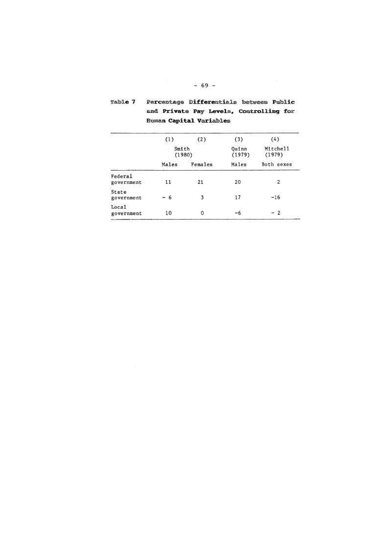
A first question is whether public sector workers

in fact get any noncompeti tive rents. The answer

depends on the study you look at, but there is

some weak evidence of positive rents. Results from

three human-capital type studies are listed in

Table 7. In each, wage levels for individuals are

regressed on age, race, sex, education, location,

and other variables, with a dummy or some other

correction for sector of employrnent. They indicate

that only for the federal governrnent, whose juris­

diction is hardest to emigrate, are rent levels

generally positive. It should be noted however

that a later analysis of Quinn (1981) shows that

other terms of the wage bargain such as pension

arrangements, disability, tenure, and job interest

are also seen to be rnore favorable for public than

private ernployees.

Other interesting evidence about wage rents cornes

from the work of Inrnan (1980) and Ehrenberg-Gold­

stein (1975). Inrnan showed that the presence of

competi tive suburbs with income levels comparable

to these in a central city implicitly, negative

values of n ~- does appear to hold down wages for

policemen and firemen by a large and statistically

significant amount. Ehrenberg-Goldstein have rein­

forced the same conclusion from a different stand­

point. They show that the union organization of

suburban employees raises central city public

wages (by reducing the credibility of private em­

ployees • exit threat), while the organization of

central city ernployees raises suburban public

wages. Both the existence of public sector rents,

- 60 -

and their negative correlation with the private

employee I s exit threat then tend to support also

the wage monopoly rationale for some degree of

excess government spending.

SUMMARY Alm LI: ~IORS

This analysis of the size and level of government

budgets in the United States thus contains some

mixed signals. On the one hand, it does not appear

that the growth of government is out of control.

In earlier decades government spending grew at

rates that exceeded those predicted on the basis

of cross-section elasticity estimates, but at

least in the seventies that has not been true for

exhaustive expenditures for national defense, and

not as true for civilian exhaustive expenditures

and transfer payrnents. And even though government

growth has not been fully explainable by cross­

section elasticity estimates, the shares of real

and nominal GNP devoted to governrnent purchases

and the labor force devoted to government employ­

ment are not particularly high by international

standards, and have been declining for a decade.

The productivity disparity, on which the Baumol

argument is based, has been responsible for a rise

in the relative price of government output of

about one percent a year for the last three de­

cades. This rise is in the official statistics

which assurnes zero productivity growth among

public ernployees, an assumption that is at least

moderately questionable for federal government

workers , though perhaps not for state and local

employees. In any case, when demand functions are

used that are more flexible than in the original

Baumol model, the rise in relative prices of

- 61 -

public output has implied essentially constant

real output shares devoted to the public sector

and only slightly rising employrnent shares. Again,

however, all public sector shares have declined in

the past decade.

But simply saying ·that government spending is not

rising at excessive rates does not imply that

spending is at its efficient level where all margi­

nal benefits of public output equal marginal

costs, or its democratically chosen median voter

level. One reason why the median voter rule might

be violated involves a whole set of "supply-side"

arguments suggesting that public employees have a

taste for more government spending, and the pos i­

tion to bring this about. lexamined carefully one

aspect of this argument, the part involving differ­

ential tastes and turnout rates of government

employees, and whether that biases electoral

fiscal outcomes. There is in fact evidence of

differential tastes and turnout rates, and this

can alter outcomes on fiscal votes, though the

actual number of cases where this has happened is

undoubtedly very small. But simply arguing that

tastes or turnout rates differ still does not

establish any voting bias unless it can also be

shown that differential tastes result from the

fact of government employment, and so far that has

not been shown.

I also examined two other hypotheses involving

more than median-voter governrnent spending levels.'

The Peltzman redistribution hypothesis might super­

ficially appear to be confirmed by the quite gener­

al voter feeling that welfare payments are too

high, but there is still a weak point in the

argument because it seems that actual beneficia­

ries of transfer programs do not vote much differ-

- 62 -

ently than anybody else (unlike public em­

ployees) , and they turn out for votes in very

small nurnbers. Hence it is not obvious that redis­

tribution-minded politicians have a winning strate­

gy -- they make some voters mad and do not make

others happy -- and therefore one would have diffi­

culty in arguing the pervasiveness of this explana­

tion of government growth.

There was slightly more evidence of some monopolis­

tic rent in public sector wage differentials, with

studies indicating that federal wages appear to be

about 10 percent above corresponding private

wages, though state and local wages appear to be

about the same as private wages. Formal models of

the wage setting process indicate why federal

wages may be somewhat higher than those at the

state-local level (there is less fear of fiscal

emigration of pr i vate taxpayer s) . But they al so

show why ultimately public employee growth and

public wage growth are substitutes, not comple­

ments, and lead to a constrained and not unbounded

overall size of the public sector.

The upshot of all this is 'that while there is some

evidence in favor of all theories of excessive

government size public employees do vote differ­

ently, welfare payments may be too high, public

wages may be excessive -- the quantitative magni­

tudes are not great and the arguments all have at

least some theoretical or empirical weak links.

The theories are interesting and at least partly

confirmed by the facts, but they have yet to make

a very compelling case that government spending

has grown to excessive proportions in the United

States.

- 63 -

ab e Est- tes of Pub1ic Expenditure D d Parameters

TS or

Study CSl Date Type el c2 ' al

Ashenfelter-Ehrenberg (1975) PCS 58-69 SL Employment .78 - .72 n.c.

Barlow (1970) CS 60 Mich. Sch. Dist. .64 - .34 n.c.

Bergstrom-Goodman (1973) CS 60 Mich. Cities .88 - .41 .98

Borcherding-Deacon (1972) CS 62 SL Agg. .83 - .76 .92

Feldstein (1975) CS 70 Mass. Sch. Dist. .48 -1.00 noc.

Gramiich (1978) TS 54-77 SL Agg'. .70 - .36 n.c.

Gramlich-Rubinfeld (1982) CS 77 Mich. Counties .40 - .06 1.01

lnman (1978) CS 68-69 N.Y. Sch. Dist. .72 n.c. n.c.

Johnson-Tomo!a (1977) TS 66-75 SL Emp. .62 - .56 n.c.

Love!! (1978) CS 70 Conn. Sch. Dist. .32 - .83 n.c.

OhIs-Wales (1972 ) CS 68 SL Agg. .74 - .11 n.c.

Mean estimate .65 - .51 .97

Standard deviation .17 .29 .02

l T8 means a time-series ana!ysis, CS a cross-section ana1ysis,and PCS a poo!ed cross-section analysis.

a 1e 2

- 64 -

xp1ained and Unexp1ained Rates of Growt:h

of Various C enb of Govenmtent SpeDding

All variables in real terms, rates of growthin per annum terms

Purchases for National Defense (G )NO

Decade

1929-39

1939-49

1949-59

1959-69

1969-79

(1 )

.179

.089

.021

-.035

(2)Predicted byEqn. (5)

n.c.

.026

.017

.022

.014

(3)

Residual

n.c.

.153

.072

-.001

-.059

(4)Share of realGNP at end

.017

.065

.107

.088

.045

Other Purchases by Federal, State, Local Government (Go)

Decade

1929-39

1939-49

1949-59

1959-69

1969-79

(1 )

d1.n GO

.034

.012

.036

.055

.028

(2)Predicted byEqn. (6)

-.007

.026

.017

.022

.014

(3)

Residua!

.041

-.014

.019

.033

.014

(4)Share of rea!GNP at end

.180

.132

.129

.149

.144

Transfer Payments, All Leve!s (T)

Decade

1929-39

1939-49

1949-59

1959-69

1969-79

(l)

d1.n T

.115

.093

.051

.067

.070

(2)Predicted byEqn. (7)

.003

.033

.031

.032

.023

(3 )

Residual

.112

.060

.020

.035

.047

(4 )Share of realGNP at end

.001

.045

.052

.067

.099

Iflable :1

- 65 -

Rates of Growth of PUblic and Priv e

• ges, Re1ative Prices for Govern:ment

ices, and Rea1 aD II' · oal Shares of

nt and OUtput Devoted to Gove nt

Rates of growth in per annum terms

l

Se

loy-

(1) (2 ) (3 ) (4 ) (5) (6 )

G/Y PG/Y E/NDecade d.R.n Wp dtn W dtn P at end at end at end l

1920-39 .003 -.001 .014 .197 .149 .172

1939-49 .020 .015 .197 .149 .155

1949-59 .023 .019 .011 .236 .200 .186

1959-69 .018 .022 .010 .237 .221 .205

1969-79 .007 .012 .010 .190 .196 .191

Average1949-79 .016 .018 .010 .215 .192 .184

l Share of full-time equivalent employment hired by the publicsector.

lf'ab1e

- 66 -

Votin Data for Various Gro

1978 Tax limit vote in Michigan

(l)

Group

1. Total

(2 )

Numberinsample

2001

(3)

Shareofelee­torate

1.000

(4 )

Turnoutrate forHeadleevote

.514

,(S)

SharevotingagainstHeadlee

.438

(6)

Mean, desiredstate tax andexp. change

%

-1.8

2. Privateworkers 1 1279

3. Not working 2 381

4. Pure pub1ic 3 186

5. Mixed4 155

6. State andlocal 5 239

7. State govt. 47

8. State univ. 25

9. Loeal govt. 64

10. School dist. 103

11. High ineome,state. 6 23

12. High income,loea1 7 31

13. Rent earning,st. or loc. 8 109

.639

.190

.093

.077

.119

.023

.012

.032

.051

.011

.015

.054

.486

.444

.683

.716

.720

.489

.600

.797

.806

.696

.903

.734

.'396

.391

.654

.496

.616

.696

.533

.588

.626

.625

.607

.700

-1.9

-1.3

-0.9

-1.5

-1.1

-1.9

-1.4

-1.3

-0.5

n.a.

n.a.

-0.4

l Includes federal government workers, who for these purposes are notin the relevant public sector.

2 Detailed breakdown is given in Table 6, rows 7, 8, and 9. Does notinclude temporarily 1aid off.

3 Respondent is single and works in the public sector, is in a house­hold where the only working spouse works in the public sector, or isin a household where both spouses work in the public sector.

4 Both spouses are working and one works in the public sector and onein the private sector.

5 Less than the sum of rows 4 and 5 because many of pure public house­holds could not be allocated.

6 All state employees with ineome above the median for state em­ployees ($16,000).

7 All loeal employees with income above the median for Ioeal em­ployees ($13,000).

8 Based on procedure described in Gramlich-RubinfeId (1982).

L

- 67 -

b1 otin iases for Different V~es

1978 Tax limit vote in Michigan

(l) (2 ) (3 ) (4) (5) (6) (7)

(Q -Q )(E V )g p g g

Election E V V Qp Qg E V +(l-E )Vg p g g g g P

l. Headlee t allpublic emp.l .170 .476 .698 .395 .580 .043

2. Headlee tst.& loc. emp.2 .119 .486 .720 .402 .616 .037

3. Headlee t rentearning emp.3 .054 .501 .734 .416 .700 .022

4. First Troymillage4 .107 .768 .797 .552 .941 .043

5. Second Troymillage 4 .107 .807 .828 .631 .962 .036

Based on the sum of rows 4 and St Table 4.

2 Based on row 6, Table 4.

3 Based on row l3 t Table 4.

4 All Q and Vestimates are based on sample probabilities andare only relatively accurate t not absolutely accurate. Hence thelevel of Vp and Vg will be off by the same amount t as will that

of Q and Qp g

more than one

lfIa.b1e 6 Voting Data for Ronpub1ic Voters

1978 Tax limit vote in Michigan

(l) (2 ) (3) (4 ) (5)Number Share of Turnout rate for Share voting

Group in sample electorate Headlee vote against Headlee

l. Private, working & not l 1660 .830 .476 .3952. Nonhomeowners 758 .379 .342 .4293. High net surplus2 451 .225 .608 .3654. Low net surplus 2 451 .225 .570 .401

5. Lansing area 3 70 .035 .386 .333

6. Not working4 381 .190 .444 .3917. Retired & disabled 18 .109 .550 .3928. Unemployed 35 .196 .536 .3339. Other 128 .064 .336 .395

O'CD

I

10. Transfer recipients 5 657 .328 .461 .44911. Social security 392 .196 .536 .46212. Unemp. ins. 6 188 .094 .436 .42713. Food stamps 109 .054 .211 .52114. AFDC & SSI (Welfare) 181 .090 .320 .43115. Working poor7 300 .150 .340 .392

Based on the sum of rows 2 and 3, Tahle 4.

2 Based on procedure described in Gramlich-Rubinfeld (1982).

All residents of counties of Lansing SMSA.

4 Same as row 3, Table 4.

5 Less than the sum of rows 11-14 because some households receive benefits fromprogram.

6 Larger than row 8 because temporary layoffs are not included in 8, and because Total includesmany on UI for a short time who were working again when the survey was taken.

7 Bottom quartile of row 2, Table 4 -- annual pretax income below tll,800.

ab e 1

- 69 -

Percentage Differentia1s bebween PDb1ic

Private Pay Leve1s. Contro11in for

B Capita1 Variab1es

(1) (2) (3) (4)

Smith Quinn Mitchell(1980) (1979) (1979)

Males Females Males Both sexes

Federalgovernment 11 21 20 2

Stategovernment - 6 3 17 -16

Localgovernment 10 O -6 - 2

- 70 -

Ashenfe1ter, O.C., and Ehrenberg, R.G. (1975).

"The Demand for Labor in the Public Sector" i

in D.S. Hamermesh (ed.), Labor in the Public

and Nonprofi t-Sectors, Princeton University

Press.

Barlow, R. (1970). "Efficiency Aspects of Local

School Expenditures II, Journal of Political

Economy, September.

Baumol, W.J. (1967). "Macroeconomics of Unbalanced

Growth: The Anatomy of the Urban Crisis II, Ame­

rican Economic Review, June.

Bergstrom, T.C.

Demand for

and Goodman, R.P. (1973). "Private

Public Goods II, _Am_e_r_i_c_a_n__E_c_o_n_o_m_1._'_c

Review, June.

Borcherding, T.E. (ed.) (1977). Budgets and Bu­

reaucrats, Duke University Press, Durham, Ne.Borcherding, T.E. (1977). IIThe Sources of Growth

of Public Expendi tures in the United States ,

1902-1970 11; in T.E. Borcherding (1977).

Borcherding, T.E., and Deacon, R.T. (1972). II The

Demand for the Services of Nonfederal Govern­

ment", American Economic Review, December.

Borcherding, T.E., Bush, W.C., and Spann, R.M.

(1977). "The Effects of Public Spending of the

Divisibility of Public Outputs in Consumption,

Bureaucratic Power, and the Size of the Tax

Sharing Group"; in T.E. Borcherding (1977).

Bowen, H. (1943). "The Interpretation of Voting in

the A11ocation of Economic ResourcesIl, Quarter­

ly Journal of Economics.

Bradford, D F., Malt, R.A., and Oates, W.E.

(1969). "The Rising eost of Loca1 Public Serv­

ices: Some Evidence and Reflections ", National

Tax Journal, June.

- 71 -

Buchanan, J.M., and Tullock, G. (1962). The Calcu­

lus of Consent, University of Michigan Press,

Ann Arbor, MI.

Bush, W.C., and Mackay, R.J. (1977). "Private

versus Public Sector Growth: A Co11ective

Choice Approach" ~ in T. E. Borcherding (1977)

Citrin, J. (1979). "Do People Want Something for

Nothing: Public Opinion on Taxes and Govern­

ment Spending" , National Tax Journal, June.

Courant, P.N., Gramlich, E.M., and Rubinfeld, D.L.

(1979). "Public Emp10yee Market Power and the

Level of Government Spending " , American Econom­

ic Review, December.

Courant, P.N., Gram1ich, E.M., and Rubinfe1d, D.L.

(1980). "Why Voters Support Tax Limitation

Amendments: The Michigan Case", National Tax

Journal, March.

Denzau, A.T., Mackay, R.J. and Weaver, C.L.(198l).

"On the Initiative-Referendum Option and the

Contro1 of Monopoly Government II , COUPE Papers

on Public Economics, No. 5.

Downs, A. (1957). An Economic Theory of Democracy,

Harper and Row, New York.

Ehrenberg, R.G., and Goldstein, G.S. (1975). ilA

Model of Public Sector Wage Determination",

Journal of Urban Economics, July.

Feldstein, M.S. (1975). "Wealth Neutrality and

Loca1 Choice in Public Education", American

Economic Review, September.

Goetz, C.J. (1977). "Fiscal Illusion in State and

Local Finance"~ in T.E. Borcherding (1977).

Gramiich, E.M. (1978). "State and Local Budgets

the Day After It Rained: Why Is The Surplus So

High?" Brookings Papers on Economic Activity,

1:1978.

- 72 -

Gramiich, E.M., and Rubinfeld, D.L. (1982).

"Voting on Public Spending: Differences be­

tween Public Employees, Transfer Recipients,

and Private Workers" , Journal of Policy Analy­

sis and Management, Summer

Hotelling, H. (1929). "Stability in Competition",

Economic Journal, March.

Inman, R.P. (1978). "Testing Political Economy's

'As If: Proposition: Is the Median Voter

Really Decisive?", Public Choice.

Inman, R.P. (1980). "Pensions, Wages, and Employ­

ment in the Loca1 Public Sector", COUPE Papers

on Public Economics, No. 4.

Johnson, G.E., and Tomola, J.D. (1977). "The Fis­

cal Substitution Effect of Alternative Ap­

proaches to Public Service Employrnent Policy",

Journal of Human Resources, Winter.

Ladd, H.F., and Wilson, J.B. (1983). "Who Supports

Tax Limitations: Evidence from Massachusetts

Proposition 2 1/2", Journal of Policy Analysis

and Management, Winter.

Lovell, H.C. (1978). "Spending for Education: The

Exercise of Public Choice", Review of Econom­

ics and Statistics, November.

Meltzer, A.H., and Richard, S.F. (1978). "Why Gov­

ernrnent Grows (and Grows) in a Demoeraey" ,

The Public Interest, Summer.

Mitchell, D.J.B. (1979). "The Impact of Co11ective

Bargaining on Compensation in the Public

Sector": in B. Aaron, J.R. Grodin, and J.L.

Stern (eds), Public Sector Bargaining, Indus­

trial Relations Research Institute.

Neufe1d, J. (1977). IITax Rate Referenda and the

Property Taxpayers' Revolt", National Tax Jour­

nal, December.

Niskanen, W.A. (1971). Bureaucracy and Representa­

tive Government, Aldine-Atherton.

- 73 -

Ohls, J.C., and Wales, T.J. (1972). IlSupp1yand

Demand for State and Loca1 Services ", Review

of Economics and Statistics, November.

Peltzman, S. (1980). Il The Growth of Government",

The Journal of Law and Economics, October.

Quinn, J. F. (1979). IlWage Differentials Among

Older Workers in the Public and Private Sec­

torsIl, Journal of Human Resources, Winter ..

Quinn, J.F. (1981). "Compensation in the Public

Sector: The Importance of Pensions? Il; in

R.H. Haveman (ed.), Public Finance and Public

Employrnent, Wayne State University Press,

1982.

Romer, T., and Rosenthal, H. (1978). "Political

Resource A1location, Contro1led Agendas, and

the Status Quo", Public Choice.

Rubinfeld, D.L. (1977). "Voting in a Local School

Election: A Micro AnalysisII, Review of Econom­

ics and Statistics.

Samuelson, P.A. (1954). "The Pure Theory of Public

Expendi ture", Review of Economics and Statis­

tics.

Smith, S. (1976). "Government Wage Differentials

by Sex II, Journal of Human Resources, Spring.

Smith, S. (1980). "Public-Private Wage Differen­

tials in Metropolitan Areas" (Mimeo).

Spann, R.M. (1977). "Rates of Productivity Change

and the Growth of State and Loca1 Governrnent

Expenditures"; in T.E. Borcherding (1977).

Tullock, G.. R. (1974). IIDynamic Hypothesis of Bu-

reaucracy", Public Choice, Fall ..

U.S. Civil Service Commission (1972). Measuring

and Enhancing Productivity in the Federal

Sector, Joint Economic Committee Print.

u.s .. Office of Personnel Management (1980). Meas­

uring Federal Productivity, Government Print­

ing Office.