theories of economic growth - bangladesh open … · theories of economic growth ... a simple...
TRANSCRIPT
UNIT TWO
THEORIES OF ECONOMIC GROWTH
This unit discusses different growth theories and models since the classical heritage. The unit covers classical growth theories in lesson-1, Marx’s model of capitalism in lesson-2, Schumpeter model on growth, development and entepreneurship in lesson-3, Harrod-Domar growth model in lesson-4, Kaldor-Mirrless (KM) model in lesson-5, neo-classical growth model in lesson-6, the Dual Economy Model in lesson-7 and finally, endogenous growth theory in lesson-8.

School of Business
Unit-2 Page-20
Blank Page

Bangladesh Open University
Economic Development and Planning Page-21
Lesson 1: Classical Heritage Objectives: Growth and development theory is at least as old as Adam Smith’s famous book published in 1776 entitled An Inquiry into the Nature and Causes of the Wealth of Nations. The macro issues of growth, and the distribution of income between wages and profits, were the major preoccupation of all the great classical economists including Adam Smith, Thomas Malthus, John Stuart Mill, David Ricardo, and Karl Marx. As for the classical theory, excepting Marx, it can be spelt in terms of its key components that bear upon growth, stationary state and the doctrine of laissez-faire.
After studying this lesson, you will be able to;
Understand the basic features of the classical theories of growth
Comprehend relevance of classical theories in the context of developing countries.
Introduction All classical economists were engaged in search for new analytical perspectives to explain growth of countries. Adam Smith gave the recognition that growth can be generated in manufacturing as well as agriculture through expansion of markets, increased specialisation of function and spurts of scientific and technical advance. Considering natural resources main constraint, Ricardo showed that output expansion slows due to diminishing marginal productivity of labour on fixed land, implying that the most productive land is brought into cultivation first, then the lesser productive, and so on. The other main ingredient in the classical era is the Malthusian idea that population expands endogenously with output. Whenever output grows, population also ill expand until average consumption drops to the level of subsistence. In other words, whenever an economy produces too much people ill procreate to expand their numbers until they revert to subsistence level (the level required for sheer physiological reproduction). According to Smith, “The premium mobile of expanding national output and labour productivity is this same extension of the market. It is this which both makes growth possible and simultaneously provides the necessary inducement not only to expand production, but to do so in a manner which increases labour productivity. Extension of the markets provides opportunities for an increase in the division of labour and division of labour raises labour productivity for three reasons: (a) workers become more efficient in the performance of particular tasks; (b) job specialisation reduces time spent switching tasks; (c) job specialisation also increases the scope for designing improved tools and machines to raise labour productivity.

School of Business
Unit-2 Page-22
For another classical, Malthus, economic growth generates increased demand for labour and hence increases wages. Rising wages in turn led to an increase in population and hence labour supply: with an increase in living standards parents choose to have more children. In Principle of Population Malthus says: "Any rise in mass living standards could only be temporary because the increase in population would rapidly outstrip the capacity of the agriculture sector to meet the growing demand for food, for additional land brought into cultivation is generally less fertile then that already cultivated." A Graphical Exposition of Classical Exposition of Classical Growth Theory
A Simple Classical Growth Model The theory of growth, as stated by the classical economists (Smith, Malthus, and Ricardo) can be described in a simple way1: According to labour theories of value, wages will be paid to each worker according to the level of subsistence and surplus. The capitalists will accumulate surplus-the difference between total products and total consumption. The surplus is assumed to be equivalent of total wage bills. Such accumulation will increase the demand for labour and with a given population, wages will tend to rise. As the wages exceeds the level of subsistence, the population will increase according to the Malthusian theory of population. Conversely, with a growth of population, the supply of labour will be encouraged and wages will again fall back to the level of subsistence. But as wages become equal to the subsistence level, a surplus will emerge to encourage to accumulation and demand for labour. The whole process will be repeated again in the next phase. The dynamics of growth ends as the law of diminishing returns sets in and wages eat up the whole production leaving no surplus for accumulation, expansion and growth population. The vertical axis measures total production minus rent and the horizontal axis measures employment of labour. The line OW indicates the subsistence wage line. With ON1 population, production is OP, wage per unit is N1 W1 and surplus or profit is El W1 when TP (total production) is the sum of wages and profits. The emergence of surplus engenders accumulation which leads to an increase in the demand for labour. Wages rise to E1N1 since the demand for labour rises with accumulation but population, and therefore labour supply, remains constant at ON1 But once the wages are above the level of subsistence, i.e. El N I > N I W1, growth of population is stimulated to ON2. 1 Based on Subrata Ghatak An International to Development Economics, London: Allen and Unwin,1986
Economic Growth
Demand for Labour
Wages Population Growth
Supply of Labour

Bangladesh Open University
Economic Development and Planning Page-23
Figure 2.2: Once the population is ON2, a 'surplus' emerges again, i.e. E2 W1 as wages are driven back to the level of subsistence and the whole process is repeated until the economy reaches a point like E where the 'stationary state’ is attained. As wages are equal to production, there is no surplus. If technical progress2 is introduced (a shift of TP to TP') then note that the point (wages = production) is only postponed, but not eliminated.
An Evaluation
One of Smith’s most important contributions was to introduce into economics the notion of increasing returns – a concept that ‘new’ growth theory (or endogenous growth theory) has recently rediscovered. In Smith, increasing returns is based on the division of labour. He saw the division of labour, or gains from specialisation, as the very basis of a social economy, otherwise everybody might as well be their own Robinson Crusoe doing everything for themselves. And it is the notion of increasing returns, based on the division of labour, that lay at the heart of Smith’s optimistic vision of economic progress as a self-generating process, in contrast to the later classical economists, such as Ricardo and 2 The introduction of technical progress and its impact will be discussed in the following growth models.
P
E2
E1 W2
W1
W TP/
TP E
Tota
l Pro
duct
ion
O N1 N2 Labour

School of Business
Unit-2 Page-24
Mill, who believed that economies would end up in a stationary state due to diminishing returns in agriculture; and also in contrast to Marx who believed that capitalism would collapse through its own ‘inner contradictions’ (competition between capitalists reducing the rate of profit; a failure of effective demand as capital is substituted for labour, and the alienation of workers).
The notion of increasing returns may sound a trivial one but it is of profound significance for the way we view economic processes. It is not possible to understand divisions in the world economy, and so-called ‘centre-periphery’ models of growth and development (between North and South and rich and poor countries), without distinguishing between activities subject to increasing returns on the one hand and diminishing returns on the other. Increasing returns means rising labour productivity and per capita income, and no limits to the employment of labour set by the (subsistence) wage, whereas diminishing returns implies the opposite. Industry is, by and large, an increasing returns activity, while land-based activities, such as agriculture and mining, are diminishing returns activities. Rich, developed countries tend to specialise in increasing returns activities, while poor developing countries tend to specialise in diminishing returns activities. It is almost as simple as that, but not quite!
As far as the extent of the market is concerned, Smith also recognised the importance of exports, as we do today particularly for small countries. Exports provide a ‘vent for surplus’; that is, an outlet for surplus commodities that otherwise would go unsold. There is a limit to which indigenous populations can consume fish, bananas and coconuts, or can use copper, diamonds and oil: “without an extensive foreign market, [manufacturers] could not well flourish, either in countries so moderately extensive as to afford but a narrow home market; or in countries where the communication between one province and another [is] so difficult as to render it impossible for the goods of any particular place to enjoy the whole of that home market which the country can afford.”
This vision of Smith of growth and development as a cumulative interactive process based on the division of labour and increasing returns in industry lay effectively dormant until the American economist, Allyn Young, based at the London School of Economics, revived it in a neglected but profound paper in 1928 entitled ‘Increasing Returns and Economic Progress’ (another paper rediscovered by ‘new’ growth theory). As Young observed: “Adam Smith’s famous theorem amounts to saying that the division of labour depends in large part on the division of labour. [But] this is more than mere tautology. It means that the counter forces which are continually defeating the forces which make for equilibrium are more pervasive and more deeply rooted than we commonly realise – change becomes progressive and propagates itself in a cumulative way.”

Bangladesh Open University
Economic Development and Planning Page-25
In Young, increasing returns are not simply confined to factors which raise productivity within individual industries, but are related to the output of all industries which he argues must be seen as an interrelated whole. Let’s give a simple example of Young’s vision of increasing returns as a macro-phenomenon. Take the steel and textile industries, both subject to increasing returns and producing price-elastic products. As the supply of steel increases its relative price falls. If demand is elastic textile producers demand proportionately more steel. Textile production increases and its relative price then falls. If demand is elastic steel producers demand proportionately more textiles, and so on. As Young says: ‘under certain circumstances there are no limits to the process of expansion except the limits beyond which demand is not elastic and returns do not increase’.
This process could not happen with diminishing returns activities, such as primary products, with demand price inelastic. No wonder levels of development, both historically and today, seem to be associated with the process of industrialisation. There is, indeed, a strong association across countries between the level of per capita income and the share of industry in GDP, and also a strong association across countries between industrial growth and the growth of GDP.
Allyn Young’s 1928 vision also got lost until economists such as Gunnar Myrdal (Swedish nobel-prize winner in economics), Albert Hirschman and Nicholas Kaldor (a pupil of Young at the LSE, and later joint-architect of the Cambridge post-Keynesian school of economists) started to develop non-equilibrium models of the development process in such books as Economic Theory and Underdeveloped Regions (Myrdal, 1957); Strategy of Economic Development (Hirschman, 1958), and Economics without Equilibrium (Kaldor, 1985).
The prevailing classical view after Smith was very pessimistic about the process of economic development which led the historian, Thomas Carlyle, to describe economics as the dismal science. The first of the pessimists was Thomas Malthus who wrote his famous Essay on Population in 1798 in which he claimed that there is a “tendency in all animated life to increase beyond the nourishment prepared for it”. According to Malthus “population, when unchecked, goes on doubling itself every 25 years, or increases in a geometric ratio [whereas] it may be fairly said – that the means of subsistence increases in an arithmetical ratio”. Taking the world as a whole, therefore, Malthus concludes that “the human species would increase (if unchecked) as the numbers 1, 2, 4, 8, 16, 32, 64, 128, 256 and subsistence as 1, 2, 3, 4, 5, 6, 7, 8, 9”. This implies, of course, a diminishing proportional rate of increase of food production, or diminishing returns to agriculture. The result of this imbalance between food supply and population will be that living standards oscillate around a subsistence level, with rising living standards leading to more children which then reduces living standards again.

School of Business
Unit-2 Page-26
This Malthusian vision forms the basis in the development literature of models of the low-level equilibrium trap associated originally with Nelson (1956) and Leibenstein (1957), and models of the big push to escape from it. The ghost of Malthus does, indeed, still haunt many Third World countries, although it has to be said that for the world as a whole, food production has grown much faster than population for at least the last century. The reason is that technical progress, always underestimated by the classical pessimists, has offset diminishing returns leading to substantial increases in productivity, particularly in Europe and North America, but also in developing countries that experienced a ‘green revolution’.
Another of the great classical pessimists was David Ricardo. In 1817 he published his Principles of Political Economy and Taxation in which he predicted that capitalist economies would end up in a stationary state with no capital accumulation and therefore no growth, also due to diminishing returns in agriculture. In Ricardo’s model, capital accumulation is determined by profits, but profits get squeezed between subsistence wages and the payment of rent to landowners which increases as the price of food increases owing to diminishing returns to land and rising marginal cost. As the profit rate in agriculture falls, capital shifts to industry causing the profit rate to decline there too. In industry, profits also get squeezed because the subsistence wage rises in terms of food. As profits fall to zero, capital accumulation ceases, heralding the stationary state. Ricardo recognised that the cheap import of food could delay the stationary state, and as an industrialist and politician, as well as an economist, he campaigned vigorously for the repeal of the Corn Laws in England which protected British farmers. Arthur Lewis’s famous model economic development with unlimited supplies of labour (Lewis, 1954) is a classical Ricardian model, but where the industrial wage stays the same as long as surplus labour exists. Ricardo’s pessimism has also been confounded by technical progress, and the stationary state has never appeared on the horizon, except, perhaps, in Africa in recent times, but the causes there are different and complex related to political failure.
Classical models of growth and distribution still form an integral part of growth and development theory, particularly the emphasis on the capitalist surplus for investment, but the gloomy prognostications of the classical economists have not materialised, at least for the capitalist world as a whole. Malthus and Ricardo both underestimated the strength of technical progress in agriculture as an offset to diminishing returns.
Limitations
1. The role of technical progress has not been captured in the model.
2. The ‘iron law of wages’, which suggests that wages cannot be above or below the level of subsistence due to Malthusian law of population, is based only on supply whereas wages are determined both by demand and

Bangladesh Open University
Economic Development and Planning Page-27
supply. It also does not take into account the role of trades unions in wage determination.
3.The Malthusian theory of population growth has been proved to be misleading in the light of the experience of economic growth of the advanced countries. The Malthusian arguments that whenever wages are above the level of subsistence, people like to have more baby rather than bicycles, radios, televisions or cars seems to be invalid both logically and empirically.
4.The classical model is too simple to account for all the complex factors which influence growth in the LDCs. For instance, labour is hardly a homogeneous input and nor is capital in the LDCs. Different types of labour and capital could affect growth differently. Accumulation need not be the sole objective function in peasant economies where people share and share alike. Also, attitudes, culture and traditional institutional values exert varying degrees of influence on growth.

School of Business
Unit-2 Page-28
Review Questions
Multiple Choice Questions 1. According to Smith, the premium mobile of expanding national output and labour productivity is:
A. Extension of the market B. Specialisation C. Laissez-faire government D. International trade
2. In Malthusian idea, economic growth generates: A. Increased demand for land and hence increases wages. B. Increased demand for labour and hence increases wages. C. Increased demand for land and hence increases rent. D. Increased demand for labour and hence increases output. 3. According to labour theory of value, wages will be paid to each worker: A. According to the level of labour-hour. B. According to the level of output and productivity. C. According to the level of subsistence and surplus. D. According to the level of profit and surplus. 4. The capitalists accumulate surplus-
A. The difference between total cost of production and total selling price.
B. The difference between total labour wage paid and totals sale of the product.
C. The difference between total investment and total consumption. D. The difference between total products and total consumption.
Answers: 1. A; 2. B; 3. C; and 4. D. Short Questions:
1. What is 'iron law of wages'? And why does it misleading?
2. Provide a graphical exposition of classical growth theory?
3. What are the limitations of limitations you find of classical theories of growth?
Essay-type Questions
1. Outline the Classical models of growth and discuss relevance for the developing countries.

Bangladesh Open University
Economic Development and Planning Page-29
2. “The notion of increasing returns may sound a trivial one but it is of profound significance for the way we view economic processes.” Discuss.
3. “Malthusian idea that population expands endogenously with output.” – analyse the relevance of such idea in the present context.
4. Explain the classical pessimism and make an evolution of it..
Further Readings
1. Mark Blaug Economic Theory in Retrospect, Delhi:Vikas Publishing, 1982
2. A N Agarwal and S P Singh (ed) The Economics of Underdevelopment, Oxford University Press, 1963
3. David Ricardo, Notes on Malthus’s Principle of Political Economy, Steffa edition, Cambridge, UK, 1951
4. T R Malthus, Principles of Political Economy, London, 1820
5. J S Mill, Principles of Political Economy,
6. Adam Smith An Enquiry into the Nature and Causes of the Wealth of Nations (1776), New York, Random House, 1937
7. David Ricardo The Principles of Political Economy and Taxation, 1817

School of Business
Unit-2 Page-30
Lesson 2: Marx’s Model of Capitalism
Objectives:
Karl Marx developed his theory of capitalistic development based on classical ideas (e.g. Ricardo's theory of value), but rejected principal features of classical theory including Malthasian law of population. Drawing his insight, the Marxian model is presented in terms of contemporary economics. The chapter also discusses the dynamic 'laws' that Marx developed.
After studying this lesson, you will be able to:
Understand Marx's Model of capitalism
Grasp dynamic laws presented by Marx
INTRODUCTION
Karl Marx in his famous book, Das Kapital (1867) predicted crisis due to falling profits, but through a different mechanism related to competition between capitalists, overproduction and social upheaval. The wages of labour are determined institutionally, and profit (or surplus value, which only labour can create) is the difference between output per man and the wage rate. The rate of profit is given by s/(v+c) or (s/v)/(1+c/v), where s is surplus value, c is 'constant' capital, v is 'variable' capital (the wage bill), and c/v is defined as the organic composition of capital. The latter is assumed to rise through time, and as it does so, the rate of profit will fall unless the rate of surplus value rises. As long as surplus labour exists (or what Marx called a ‘reserve army of unemployed’) there is no problem, but Marx predicted that as capital accumulation takes place, the reserve army will disappear, driving wages up and profits down. The capitalists’ response is either to attempt to keep wages down (the immiseration of workers) leading to social conflict, or to substitute more capital for labour which raises the organic composition of capital and worsens the problem of a falling profit rate. Moreover, as labour is substituted, it cannot consume all the goods produced, and there is a failure of effective demand, or a ‘realisation crisis’ as Marx called it. Capitalism collapses through its own ‘inner contradictions’, and power passes to the working classes.
MARX’S MODEL OF CAPITALISM3:
Karl Marx (1818-83) advocated a unique theory of capitalist economic development, which is similar to Ricardo's, even though underlying assumptions and policy implications are diametrically relates to opposite.
3 Based on Yujiro Hayami Development Economics, Oxford: Oxford University Press, 1988.

Bangladesh Open University
Economic Development and Planning Page-31
Similarity between Marx and Ricardo labour supply to the modern industrial sector which is infinitely elastic at an institutionally determined subsistence wage rate. These works as a basic support for rapid capital accumulation. Rejecting the Malthusian population law as the mechanism for producing the infinitely elastic labour-supply curve, Marx build his theory on the existence of the 'surplus' labour force which he termed 'industrial reserve army'4. As long as this reserve army exists, the industrial wage rate is prevented from rising above the subsistence level.
The basic assumption of the Marxian model is that the industrial reserve army will never be exhausted, as it is reproduced in the capitalistic development process. The number of people ousted from traditional occupations continue to increase as the capitalist sector expands, replenishing the industrial reserve army. On the other hand, capitalists always try hard to substitute capital for labour through mechanisation. As a result, employment in the modern industrial sector increases more slowly than the speed of capital accumulation and output growth. This slow employment growth in the modern sector is counteracted by additional entries to the reserve army from the traditional sector. Thus diffusing from Malthus, Marx postulates that the horizontal labour supply curve to capitalist entrepreneurs is not a product of natural population law, but the consequence of capitalism incessantly reproducing the industrial reserve army.
The Marxian model is reconstructed in the terms of modern economics in the following figure 2.3. The vertical and horizontal axis measure the wage rate and employment respectively. DD represents a labour demand curve, corresponding to a schedule of labour's marginal value product for a given stock of capital.
The labour supply curve (S1) drawn horizontally at the subsistence wage rate (W). However, while Ricardo's labour supply is, assumed to be indefinitely, horizontal in the long run owing to the Malthusian population law, Marx's begins to rise from a certain point (Ro) which represents exhaustion of the industrial reserve army.
4 The reserve army consists of lumpen proletariat in urban slums who stake out a bare living from various informal activities (from petty trade to pilferage), while seeking formal employment in the industrial sector. As such, they are readily available to accept employment at the subsistence wage rate upon recruitment by industrial employers.

School of Business
Unit-2 Page-32
Figure 2.3: The Marx Model of Capitalist Economic Development
Assume that in an initial period (0) a labour demand curve for the modern capitalist sector is located at line Do corresponding to capital stock (Ko). The initial equilibrium is established at point A with labour employed by OLo at the subsistence wage rate OW. However, according to Marx's assumption, the number of labourers seeking employment in the modern industrial sector measured by WR0 is larger than OL0. Those unable to find employment remain engaged in informal activities in urban slums, awaiting the opportunity to be employed in the capitalist sector. This population, as measured by ARo, is the industrial reserve army of Marx's definition. Therefore, increases in labour demand corresponding to capital accumulation do not result in an increase in the wage rate until point Ro is reached. Unlike Ricardo's long-run labour supply curve, which is indefinitely horizontal, Marx's curve begins to rise from point Ro implying that capitalists have to offer higher wage rates to attract labourers when the reserve army is exhausted. However, in his model the reserve army is never drained. First, in the process of capitalist development, small self-employed producers in traditional agriculture and cottage industries fall to the rank of industrial reserve army. As capitalist increase in capital stock from K0 to KI, the output of their enterprises expands from area AD0OL0 to BD1OL1.Outcompeted by this expansion in capitalist production, traditional self-employed producers and their family members are forced to seek employ-ment in the capitalist sector, resulting in the elongation of the horizontal portion of labour supply curve to RI.
(W)
D1
S0 D0
A B
L0 L1
D0 (K0)
D1 (K1)
(L)
O
R0 R1
S1
W Wag
e R
ate
Labour Employment

Bangladesh Open University
Economic Development and Planning Page-33
With bias for the technological progress embodied in new machinery, the increase in employment from OL0 to OL1 became slower than the growth of output from area AD0LOo to BD1OL1. Marx envisioned that the industrial reserve army would never be exhausted, with the ability of the modern capitalist production system to ruin traditional self- employed producers, together with the labour-saving bias in industrial technology. The process of capitalist development, as described by Marx, necessarily involves rapid increases in inequality of income distribution. Unlike Ricardo's case-where the wage rate can rise in the short run until the population adjusts to demand increases in the process of capital accumulation-no such possibility exists for industrial workers. The labourers' wage share income in total savings output decreases from AWOL0/AD0OL0 to BWOL1/BD1OL1, while the share of capitalists' profit rises from ADoW/ AD0OL0 to BD1W/BD1OL1. Marx predicted that increasing inequality in the capitalist economy would ignite contradiction between labour and capitalist. This inherent contradiction of capitalist development, according to Marx, eventually leads to violent revolution. The revolution will replace capitalism by socialism Marxian Theory: A Summary The Marxian model of economic growth depends on some major dynamic ‘laws.’ First, the law of capitalistic accumulation which says that prime desire of the capitalists is to accumulate more and more capital. Second, the law of falling tendency of the rate of profit which plays a crucial role in the breakdown of the capitalistic system. Third, the law of increasing concentration and centralisation of capital which illustrates the growth of capitalism, cut-throat competition amongst capitalists will lead to the annihilation of smaller firms by larger ones which would lead to the growth of monopoly and concentration of economic power. Fourth, the law of increasing ‘pauperisation’ which implies the growth of the misery of the working class with the advancement of capitalism, that would be reflected in wages being tied to the subsistence level coupled with the rise in the proportion of unemployed people. On the problems of developing countries, Marx analysis was rather thin. Marx paid some attention to Indian economic problems. According to his critics, what is wrong with Marx is that he first of all confused money and real wages, and secondly underestimated the effect of technical progress in industry on the productivity of labour. A rise in money wages as labour becomes scarcer does not necessarily mean a rise in real wages; and a rise in real wages could be offset by a rise in productivity, leaving the rate of profit unchanged, they added. In other words, in a growing economy, there is no necessary conflict between wages and the rate of profit.

School of Business
Unit-2 Page-34
Review Questions
Multiple Choice Questions 1. The basic assumption of the Marxian model is that the industrial
reserve army will:
A. never be exhausted.
B. not remain stable.
C. be exhausted.
D. have limited supply.
2. The labour supply curve in the Marxian model is drawn:
E. indefinitely horizontal.
F. horizontally.
G. indefinitely vertical.
H. vertical.
3. The process of capitalist development, as described by Marx, necessarily involves:
I. rapid increases in equality of income distribution.
J. rapid increases in equality of income growth.
K. rapid increases in inequality of income distribution.
L. rapid increases in income distribution.
4. In Ricardian case the wage rate can:
a. decline in the short run
b. rise in the long run
c. decline in the long run
d. rise in the short run
Answers: 1. A; 2. B; 3. C and 4. D
Short Questions
1. What are the differences between Marx and Ricardo in relation to labour supply?
2. What is prediction of Marxian model of capitalistic development?
Essay-type Questions
1. Karl Marx advocated a unique theory of capitalist economic development, which is similar to Ricardo's even though underlying assumptions and policy implications are diametrically relates to opposite– Discuss.
2. The Marxian model of economic growth depends on some major dynamic ‘laws.’ – explain the laws.
Bangladesh Open University
Economic Development and Planning Page-35
3. How far do you think the Marxian model of economic growth is realistic?
Further Readings
1. Ghatak, S. 1986. An Introduction to Development Economics. Allen & Unwin. London.
2. Marx, K (1887) Capital, Vol I
3. Marx, K (1893) Capital, Vol II
4. Marx, K (1894) Capital, Vol III
5. Marx, K (1859) A Contribution to the Critique of the Political Economy

School of Business
Unit-2 Page-36
Lesson 3: Schumpeter on Growth, Development and Entrepreneurship
Objectives:
Schumpeter,5according to some economic historian, disassociated himself from the classical growth theorists and made an effort to distinguish between growth and development. Schumpeter postulates that development is an innovatory process while he illustrates growth as rather a slow and insignificant process, emanating from investment of additional capital financed by reinvestment of profits. He also distinguishes between producer capitalist and entrepreneurship. Schumpeter provides the idea of ‘creative destruction’.
After studying this lesson, you will be able to:
Underestimate the ideas of Schumpeter on growth, development and entrepreneurship.
Introduction
Joseph Alois Schumpeter (1883-1950), in 1911 published the first German edition of his analysis of economic development, departing from the classical economists who primarily concentrated on economic growth, focusing on the expansion of market, saving and investment. In Schumpeterian scheme, development in capitalism hinges upon the entrepreneurs who introduce innovations, causing shifts in some or other production function.
Economic growth and development.
Schumpeter draws a clear distinction between economic growth and development. Economic growth, according to him, is a gradual process of expansion of production and repetition of the same applying the same methods. On the contrary economic development is simultaneously a more dramatic and disruptive process. Economic development calls for of the carrying out of 'new combinations of productive means'. According to him, such a new combination would either lead to transformation the conditions of production of existing goods and/or introduction of new goods. The process requires to open up new sources of supply or new markets or reorganisation of an industry (e.g, the creation of a monopoly position or the breaking up of a monopoly position).
Schumpeter characterises production methods, products, markets, and industrial organisation as aspects of economic development which give rise to 'productive revolutions'. He uses the phrase to emphasise transforming aspect of development. 5 Schumpeter, J (1911), The Theory of Economic Development, Oxford: Oxford University Press, 1961. His other major publications include Business Cycles (1939), Capitalism, Socialism and Democracy (1942), and History of Economic Analysis which appeared posthumously and unfinished in 1954.
Bangladesh Open University
Economic Development and Planning Page-37
A central aspect of Schumpeters analysis is his specification of the three common features which, in his view, are inherent in most instances of economic development, and without which that development cannot generally occur. These three essential features are as follows:
1. The mobilisation of existing factors of production and their combination in new ways.
2. Extension of credit which is generally essential in order to provide the necessary command over factors of production in the market.
3. The presence or an economic entrepreneur, which is a sina qua non for the initiation or this process of resource mobilisation and for carrying it through to completion.
For Schumpeter the essential feature of economic development is not the incremental accumulation of new capital, but the mobilisation or existing factors for new uses. Schumpeter notes: “As a rule the new combinations must draw the necessary means or production from some old combinations. Different methods or employment and not saving and increases in the available quantity or labour, have changed the race or the economic world in the last fifty years."
If new combinations of factors of production are carried out by existing firms, or by individuals with substantial wealth, then a problem of finance may not arise. The initiators of the new combinations may either already have the necessary factors, or be able to buy them. However, Schumpeter argues, the situation is usually different. Firstly, 'new combinations are, as a rule, embodied, as it were, in new firms. ….in general it is not the owner or stage-coaches who build railways'. Secondly, even large firms usually need extra finance to implement this type of innovation.
Capitalist and entrepreneur
Making distinction between capitalist and entrepreneurs, Schumpeter says that the capitalist provides the finance, and carries the risk, or economic development, but he does not bring it about. This is done by the entrepreneur some one who has the foresight to perceive new opportunities and to takes the initiative to pursue them.
According to Schumpeter an entrepreneur is a person who "actually carries out new combinations, and loses the character as soon as he has built up his business, when he settles down to running it as other people run their businesses."
For Schumpeter, the critical feature of economic development is not mobilisation of savings by capitalists to finance the accumulation or more productive capital, but the actions of entrepreneurs in mobilising credit to finance the procurement of existing factors of production in order to combine them in new ways. Innovation lies at the heart of development, and the innovator is the entrepreneur.

School of Business
Unit-2 Page-38
Schumpeter and endogenous growth theory
Three particular aspects of Schumpeter's work figure prominently in one strand of endogenous growth theory. One is the notion of clusters of innovation which are heavily associated with externalities in the production and/or use of knowledge as in technological spillovers. Second, reference is made to imperfect competition and the extent to which the benefits of innovation accrue in the form of rents to the firms concerned. If innovation spreads quickly so does the general level of productivity. Third, Schumpeter is a source of dynamics, with waves of creation and, at times, destruction.
In short, endogenous growth theory as a theory of productivity increase has two bountiful and overlapping sources for ideas which can be incorporated in one or another way into a formal model and be tested empirically. Either ideas, usually piecemeal and most notably from Schumpeter, can be purloined from earlier literature, or a more or less arbitrary but highly specific source of technical change is casually invented through some economic mechanism attached to human capital, produced R&D, or spill-over. On this basis, the theory is able to broaden its scope of application and even putatively confront a range of policy issues.

Bangladesh Open University
Economic Development and Planning Page-39
Review questions Multiple Choice Questions 1. In Schumpeterian scheme, development in capitalism hinges upon:
A. the entrepreneurs. B. the capitalists. C. the firms. D. the production function.
2. For Schumpeter, the critical feature of economic development is A. mobilisation of savings by capitalists B not mobilisation of savings by capitalists. C. mobilisation of capital by capitalists D. mobilisation of savings by entrepreneurs.
Answers: 1. A; and 2. B. Short questions
1. How does Schumpeter draw a distinction between economic growth and development?
2. What are the common features that, according to Schumpeter, remain inherent in most instances of economic development?
3. What are the differences between Schumpeterian view and the classical vantage on economic growth?
4. What are the particular aspects of Schumpeter's work figure prominently in one strand of endogenous growth theory?
Essay-type Questions
1. Economic development is simultaneously a more dramatic and disruptive process – Discuss.
2. For Schumpeter, the critical feature of economic development is not mobilisation of savings, but the actions of entrepreneurs – Explain.
Further Readings 1. Ghatak, S. 1986. An Introduction to Development Economics. Allen
& Unwin. London. 2. Hayami ,Y. 1987. Development Economics. Clarendon Press.
Oxford. 3. Hoff, K., Braverman, A., and Stiglitz, J. 1993. The Economics of
Rural Organization .published for the World Bank. Oxford University Press

School of Business
Unit-2 Page-40
Lesson 4: Modern Growth Models: Harrod-Domar Growth Model- A Keynesian Variant
Objectives:
The last 50 years of 20th century have witnessed a remarkable increase in the development of theories of economic growth which attempt to show how the structure of a country’s economy is expected to change when factors determining the rate of growth changes. Proliferation of these theories coincided with the end of Second World War together with the 1930s international economic recession, which witnessed emergence of a new brand in economic theory, popularly known as 'Keynesian Economics'. These theories base on the Keynesian perspective of emphasising the role of aggregate demand as the engine of growth. Harrod6 and Domar gave birth to modern growth model in accordance with Keynesian perspective. Harrod (1939) provides a dynamic dimension to Keynesian economics which is also implicit in Domar.
After studying this lesson, you will be able to:
Understand the process of growth as envisioned by Harrod and Domar.
Realize the implication of Harrod-Domar Model in Developing Countries
Introduction
For nearly sixty years after Marx’s death in 1883, growth and development theory lay virtually dormant until it was revived by the British economist (Sir) Roy Harrod in 1939 in a classic article ‘An Essay in Dynamic Theory’ in Economic Journal,March,1939. In the late 19th and early 20th centuries, economics was dominated by neoclassical value theory under the influence of Jevons, Walras and particularly Alfred Marshall’s Principles of Economics published in 1890. Growth and development was regarded as an evolutionary natural process akin to biological developments in the natural world. All this changed in 1939 with Harrod’s article, which led to the development of what came to be called the Harrod-Domar growth model (named after Evesey Domar as well who derived independently Harrod’s fundamental result in 1947 but in a different way (Domar, 19477).) The model has played a major part in thinking about development issues ever since, and is still widely used as a planning framework in developing countries. Neoclassical growth theory was born as a reaction to the Harrod-Domar model, and ‘new’ growth theory developed as a reaction to neoclassical growth theory. 6 Harrod was one of the most original and versatile economists of the twentieth century. He was the inventor of the marginal revenue product curve in micro theory; the life-cycle hypothesis of saving and the absorption approach to the balance of payments in macro theory; the biographer of Keynes; the author of a book on inductive logic, as well as the originator of modern growth theory 7 Domar,E,'Expectation and Employment', American Economic Review, Vol-37, March,1947

Bangladesh Open University
Economic Development and Planning Page-41
Harrod-Domar Growth Model
Harrod’s 1939 model was an extension of Keynes’s static equilibrium analysis of The General Theory. The question Harrod asked was: if the condition for a static equilibrium is that plans to invest must equal plans to save, what must be the rate of growth of income for this equilibrium condition to hold in a growing economy through time? Moreover, is there any guarantee that this required rate of growth will prevail?
Harrod introduced three different growth concepts: the actual growth rate (ga); the warranted growth rate (gw) and the natural growth rate (gn). The actual growth rate is defined as ga = s/c, where s is the savings ratio and c is the actual incremental capital-output ratio (i.e. the amount of extra capital accumulation or investment associated with a unit increase in output). This expression is definitionally true because in the national accounts, savings and investment are equal. Thus s/c = (S/Y)/(I/Y) = (Y/Y), where S is saving, I is investment, Y is output, and Y/Y is the growth rate (ga).
This rate of growth, however, does not necessarily guarantee a moving equilibrium through time in the sense that it induces just enough investment to match planned saving. Harrod called this rate the warranted growth rate. Formally, it is the rate that keeps capital fully employed, so that there is no overproduction or underproduction, and manufacturers are therefore willing to carry on investment in the future at the same rate as in the past. How is this rate determined? The demand for investment is given by an accelerator mechanism (or what Harrod called ‘the relation’) with planned investment (Ip) a function of the change in output, so that Ip = crY, where cr is the required incremental capital-output ratio at a given rate of interest, determined by technological conditions. Planned saving (Sp) is a function of income so that Sp = sY where s is the propensity to save. Setting planned investment equal to planned saving gives crY = sY or Y/Y = s/cr, which equals the warranted growth rate (gw). For dynamic equilibrium, output must grow at the rate s/cr. If not, the economic system will be cumulatively unstable. If actual growth exceeds the warranted growth rate, plans to invest will exceed plans to save; and the actual growth rate is pushed even further above the warranted rate. Contrawise, if actual growth is less than the warranted rate, plans to invest will be less than plans to save and growth will fall further below the warranted rate. This is the Harrod instability problem. Economies appeared to be poised on a ‘knife-edge’. Any departure from equilibrium, instead of being self-righting, will be self-aggravating.
The American economist, Evesey Domar, working independently of Harrod, also arrived at Harrod’s central conclusion by a different route – hence the linking of their two names. What Domar realised was that investment both increases demand via the Keynesian multiplier, and also increases supply by expanding capacity. So the question he posed was: what is the rate of growth of investment that will guarantee that demand matches supply? The crucial rate of growth of investment can be

School of Business
Unit-2 Page-42
derived in the following way. A change in the level of investment increases demand by Yd = I/s, and investment itself increases supply by Ys = I, where is the productivity of capital (Y/I). Therefore, for Yd = Ys we must have I/s = I, or I/I = s. That is to say, investment must grow at a rate equal to the product of the savings ratio and the productivity of investment. With a constant savings-investment ratio, this implies output growth at the rate s. Since = 1/cr (at full employment), then the Harrod and Domar result for equilibrium growth is the same.
Even if the actual and warranted growth rates are equal, however, guaranteeing the full utilisation of capital, this does not guarantee the full utilisation of labour which depends on the natural rate of growth (gn) made up of two components: the growth of the labour force (l) and the growth of labour productivity (t), both exogenously given. The sum of the two gives the growth of the labour force in efficiency units. If all labour is to be employed, the actual growth rate must match the natural rate. If the actual growth rate falls below the natural rate there will be growing unemployment of the structural variety.
It should be clear that the full employment of both capital and labour requires that ga = gw = gn; a happy coincidental state of affairs that Joan Robinson once coined ‘the golden age’ to emphasise its mythical nature.
Harrod-Domar Model and Developing Countries
Where do the developing countries fit into this story? The short-run (trade cycle) problem is the relation between ga and gw, and we won’t say more about this here. The long run problem is the relation between gw and gn, or the relation between the growth of capital and the growth of the labour force in efficiency units. Almost certainly, in most developing countries, gn exceeds gw. Labour force growth (determined by population growth) may be 2 percent per annum, and productivity growth 3 percent per annum, giving a natural growth rate of 5 percent. If the net savings ratio is 9 percent and the required incremental capital-output ratio is 3, the warranted growth rate is only 3 percent. Therefore gn > gw. This has two main consequences. Firstly, it means that the effective labour force is growing faster than capital accumulation so that with fixed coefficients of production there will be unemployment of the structural variety. Secondly, it means that plans to invest will exceed plans to save, because if the economy could grow at 5 percent there are profitable investment opportunities for more than 9 percent saving, and there will be inflationary pressure. Hence, the simultaneous existence of unemployment and inflation in developing countries is not a paradox; it is the outcome of an inequality between the natural and warranted growth rates.
A good deal of development policy can be understood and considered within this Harrod framework. The task is to bring gn and gw closer together; to reduce gn and to increase gw. The only feasible way to reduce the growth of the labour force is to reduce population growth.

Bangladesh Open University
Economic Development and Planning Page-43
The Harrod model provides a rationale for population control. A second way to reduce gn is to reduce the rate of labour saving technical progress, but this has the serious drawback of reducing the growth of living standards. A rise in gw could be brought about by increases in the savings ratio. This is what monetary and fiscal policy programmes are designed to do, with emphasis on tax reform and policies of financial liberalisation. A rise in gw could also come about if the capital-output ratio was reduced by countries using more labour intensive techniques of production. There is an on-going debate on the choice of appropriate techniques in developing countries, and whether more labour intensive techniques could be employed without the sacrifice of output or saving.
Debates in growth economics
The Harrod (and Domar) model provided the starting point for the great debates in growth economics that preoccupied large sections of the economics profession for at least three decades between the mid-1950s and the 1980s. The battle-lines were drawn up between the neoclassical growth school on the one hand based in Cambridge, Massachusetts, USA with the major protagonists being Robert Solow, Paul Samuelson and Franco Modigliani, and the Keynesian growth school on the other based in Cambridge, England with the major protagonists being Nicholas Kaldor, Joan Robinson, Richard Kahn and Luigi Pasinetti. What was immediately apparent to both camps was that if the Harrod-Domar model was a representation of the real world, all economies, rich and poor, capitalist and communist, would be in for a bumpy ride. The variables and parameters determining gn and gw were all independently given, and there were apparently no automatic mechanisms for bringing the two rates of growth into line to provide the basis for steady long run growth at the natural rate. The task that both conflicting camps set themselves was to develop mechanisms to reconcile divergences between gn and gw.
The Cambridge, England camp focussed on the savings ratio, making it a function of the distribution of income between wages and profits which in turn was assumed to be related to whether the economy was in boom or slump. Specifically in their model the propensity to save out of profits is assumed to be higher than out of wages, and the share of profits in national income is assumed to rise during booms and fall during slumps. Therefore, if gn exceeds gw, generating a boom, the share of profits rises and the savings ratio will rise raising gw towards gn. The only constraint might be an ‘inflation barrier’ caused by workers not being willing to see the share of wages fall below a certain minimum. Conversely, if gn is less than gw, generating a slump, the share of profits falls and the savings ratio falls lowering gw towards gn. The only limit here might be a minimum rate of profit acceptable to entrepreneurs which sets a limit to the fall in the share of profits.
The Cambridge, Massachusetts camp focussed on the capital-output ratio arguing that if the labour force grows faster than capital, the price mechanism will operate in such a way as to induce the use of more

School of Business
Unit-2 Page-44
labour intensive techniques, and vice versa. Thus if gn exceeds gw, the capital-output ratio will fall raising gw to gn. If gn is less than gw, the capital-output ratio will rise lowering gw to gn. This neo-classical adjustment mechanism, however, presupposes two things. Firstly, that the relative price of labour and capital are flexible enough, and secondly that there is a spectrum of techniques to choose from so that economies can move easily and smoothly along a continuous production function relating output to the factor inputs, capital and labour. If this is true, economies can achieve a growth equilibrium at the natural rate.
Out of the neo-classical model, however, came the extraordinary counterintuitive conclusion that investment does not matter for long run growth because the natural rate depends on the growth of the labour force and labour productivity (determined by technical progress) and both are exogeneusly determined. Any increase in a country’s saving or investment ratio would be offset by an increase in the capital-output ratio leaving the long run growth rate unchanged. The argument depends crucially, however, on the productivity of capital falling as the capital to labour ratio rises. In other words, it depends on the assumption of diminishing returns to capital. This is the neo-classical story that ‘new’ endogenous growth theory objects to. If there are mechanisms which keep the productivity of capital from falling as more investment takes place, then the investment ratio will matter for long run growth, and growth is endogenous in this sense i.e. growth is not simply determined by the exogenous growth of the labour force in efficiency units.
Criticism Based on Evidence
A major problem in the Harrod-Domar model is the fixed relationship which states that output must grow at par with capital in the long term. This fixed relationship between capital and output: y= l/v K. The constant capital/output ratio implies that the percent changes in capital stock and output must be equal. However, for a wide cross section of LDCs, y>k. Growth accounting studies find that, roughly, net capital growth is K =2%, while y = 4.5%. Therefore it is invalid for Harrod-Domar to assume that increased capital is the only source, or even the primary source, of growth. Obviously other important sources of growth are subsumed in the parameter v. For example, there can be increments in productive labour, skills, technological improvements, and soon. Studies in the 1960s empirically determined the sources of growth for the United States to be roughly as follows, with the residual attributed to technological progress.
The Harrod-Domar model is also criticised because its implied growth is seen as inherently unstable. This instability arises from the mismatch between the rates of growth of capital and labour force. Recall that modern growth models differ from the classical model in assuming that L grows exogenously-it is independent of income growth. But how will an annual population growth rate of 3% match with a 2% rate of growth of the capital stock? If these two rates diverge, a mismatch must emerge between capital stock and the labour required to run the machines. There is no reason for the labour growth rate to equal output growth s/ v, except
Bangladesh Open University
Economic Development and Planning Page-45
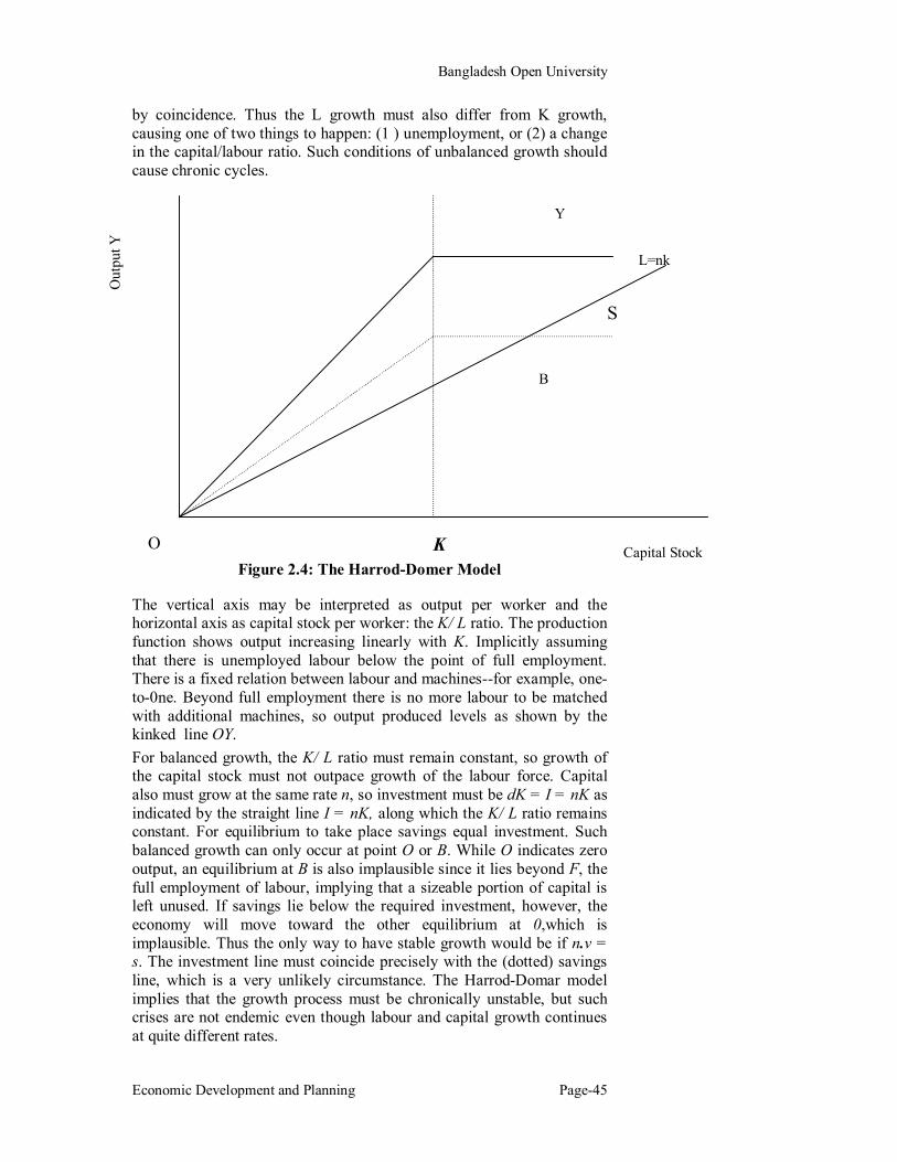
by coincidence. Thus the L growth must also differ from K growth, causing one of two things to happen: (1 ) unemployment, or (2) a change in the capital/labour ratio. Such conditions of unbalanced growth should cause chronic cycles.
Y
Figure 2.4: The Harrod-Domer Model The vertical axis may be interpreted as output per worker and the horizontal axis as capital stock per worker: the K/ L ratio. The production function shows output increasing linearly with K. Implicitly assuming that there is unemployed labour below the point of full employment. There is a fixed relation between labour and machines--for example, one-to-0ne. Beyond full employment there is no more labour to be matched with additional machines, so output produced levels as shown by the kinked line OY. For balanced growth, the K/ L ratio must remain constant, so growth of the capital stock must not outpace growth of the labour force. Capital also must grow at the same rate n, so investment must be dK = I = nK as indicated by the straight line I = nK, along which the K/ L ratio remains constant. For equilibrium to take place savings equal investment. Such balanced growth can only occur at point O or B. While O indicates zero output, an equilibrium at B is also implausible since it lies beyond F, the full employment of labour, implying that a sizeable portion of capital is left unused. If savings lie below the required investment, however, the economy will move toward the other equilibrium at 0,which is implausible. Thus the only way to have stable growth would be if n.v = s. The investment line must coincide precisely with the (dotted) savings line, which is a very unlikely circumstance. The Harrod-Domar model implies that the growth process must be chronically unstable, but such crises are not endemic even though labour and capital growth continues at quite different rates.
Out
put Y
Capital Stock
L=nk
B
O K
S

School of Business
Unit-2 Page-46
Review Questions Multiple Choice Questions
1. Harrod introduced three different growth concepts: A. the actual growth rate; the warranted growth rate and the natural
growth rate. B. the equilibrium growth rate; the warranted growth rate and the
natural growth rate. C. the stationary growth rate; the warranted growth rate and the
natural growth rate. D. the actual growth rate; the steady state growth rate and the
natural growth rate. 2. The simultaneous existence of unemployment and inflation in
developing countries, according to Harrod-domar Model: A. is a paradox; it is the outcome of an equality between the natural
and warranted growth rates. B. is not a paradox; it is the outcome of an inequality between the
natural and warranted growth rates. C. is a paradox; it is the outcome of an inequality between the
natural and warranted growth rates. D. is not a paradox; it is the outcome of an equality between the
natural and warranted growth rates. 3. The Cambridge, England camp focussed on:
A. the capital ratio. B. the capital-output ratio. C. the savings ratio. D. the output ratio.
4. The Cambridge, Massachusetts camp focussed on: A. the capital ratio. B. the output ratio. C. the savings ratio. D. the capital-output ratio.
Answers: 1. A; 2.B; 3.C and 4. D
Short Questions 1. What is the Harrod instability or knife-edge problem?
2. What are three growth concepts Harrod introduced?
3. What did the Cambridge, USA focus on?
4. What did the Cambridge, UK focus on?
5. What does the Harrod-Domar model offer for the analysis of development policy?

Bangladesh Open University
Economic Development and Planning Page-47
Essay-type Questions
1. "Prime mover in the economy is the investment"-analyse the statement.
2. Do you agree with the statement that gross output at the same rate as capital in the long run?
3. If the labour force grows faster than capital, the price mechanism will operate in such a way as to induce the use of more labour intensive techniques, and vice versa.
4. Outline the Harrod-Domar Model. Discuss the possible uses and limitations of the model for developing countries.
Further Readings 1. Hayami ,Y. 1987. Development Economics. Clarendon Press.
Oxford.
2. Romer D, Advanced Macroeconomics, New York: McGrawhill, 1996.
3. Maddison, Angus. 1982. Phase of Capitalist Development. Oxford: Oxford University Press.
4. Mankiw, N. Gregory. 1994. Macroeconomics. Second Edition. New York: Worth
5. Barro, Robert J., and Salai-I-Martin, Xavier. 1991."Convergence Across states and regions". Brookings Paper on Economic Activity, no.1, 107-182.
6. Barro, Robert J., Mankiw, N. Gregory, and Salai-I-Martin, Xavier. 1995."Capital Mobility in Neoclassical Models of Growth ". American Economic Review 85 (March) : 103 -115.
7. Kasiwal, Pari. 1995. Development Economics.. South-Western College Publishing.
8. Ghatak, S. 1986. An Introduction to Development Economics. Allen & Unwin. London.

Lesson 5: Kaldor-Mirrless (KM) Model
Objectives:
The Kaldor-Mirrless (KM)8 model introduces a technical progress function. According to the KM, saving ratio can be made flexible to obtain a steady sate economic growth. Like the Harrod- Domar model the capital-output ratio remains fixed as opposed to the neo-classical model. Moreover Kaldor's introduction of 'alternative' theory of distribution into the model stimulates analysis of the problems of economic growth. After studying this lesson, you will be able to: Understand the KM model of economic growth Explain the drawbacks of the KM model
Introduction
Kaldor has discussed the idea of economic growth in several essays. He precisely deals with economic growth in two essays published in 1957 and 1962. He published the second one with James Mirless, a Nobel laureate. There are several distinctive feature of KM model:
For obtaining a steady state economic growth, the saving ratio can be made flexible.
The capital output ratio remains fixed, like Harrod Domar model, in contrast to neoclassical model.
The KM introduces a technical progress function, discarding the production function approach of neoclassical theory.
An investment function is specified in the KM model, unlike the neoclassical school.
The KM dropped both assumptions relating to full employment and perfect competition.
The model introduces an 'alternative' theory of distribution to analyse the problem of economic growth.
Kaldor-Mirrless (KM) Model 9
The KM begins with assumption that total income (Y) is equal to the sum of wages (W) and profits (P)
or Y = W + p--------------------------------------(1) Total savings (S) are assumed to be equal to savings our of wages (Sw) and profits (Sp) or S =Sw+ Sp -------------------------------------(2)
8 Kaldor,N and Mirrless,J,' Anew Mode of Economic Growth', Review of Economic Studies,pp 174-92 Kaldor,N 'A Model of Economic Growth', Economic Journal, 67,pp591-624, 1957. 9 Based on S. Ghatak An Introduction to Development Economics, London: Alklen &Urnwin,1986.
Bangladesh Open University
Economic Development and Planning Page-49
Note that S = swW + spP .--------------------------------------(3) and Sw = sw W ------------------------------------(4)
Sp = sp P -------------------------------------(5) Where sw = propensity to save by wage earners
sp = propensity to save by profit earners S = total savings
Both sw and sp are assumed to be constants indicating the equality between marginal and average propensities. Now Y = W + P-------------------------------(6) And S = sw W + sp P------------------------(7) By substitution, we have,
S = sw (Y -P) + sp P ------------------------(8) S = (sp - sw)P + sw.Y -----------------------(9)
Since it is assumed that I = S we have,
I = (sp - sw)P + sw.Y -----------------------(10)
Dividing the both sides of the equation by Y, and rearranging, we obtain, P/Y =[1/ {sp-sw } .1/Y]- [sw/{sp-sw}]------------------(11) Thus, the profit share of income is given by the share of investment to income. The stability of the model is given by 0 < s w < s p <1 Notice that the flexibility of saving is achieved in the KM- model by the assumption of different propensities to save by wage and profit earners. The specific value of savings necessary to obtain the solution would be given by income distribution between income classes. Given sp and sw, I/Y will determine P/Y. If it is assumed that sw. = 0, we then obtain
P/Y = 1/sp .1/Y---------------------------------(12) Note that if the capital-output (K/Y) is fixed as in the Harrod Domar (HD) model, we can write, [P/Y] .[Y/K] =[1/sp] .[1/Y] .[Y/K]----------------------(13) or [P/K] =[1/sp] . [1/K]--------------------------------------(14)
School of Business
Unit-2 Page-50
Since P/K = V, or the rate of profit earned on capital and,
I/K = J, or the rate of accumulation, we have.
V = 1/sp . J-------------------------------------(15)
or sp .V = J ----------------------------------------(16) If sp = 1. all profits are saved in the equilibrium and we get
V = J (=n)----------------------------(17) Where n = the natura1 growth rate, Thus the rate of growth is given by the rate of profit which is determined by the propensities to save of the profit earners. Criticisms Several important criticisms have been levelled against the Kaldorian theory of economic growth. First, the model, according to Pasinetti allows workers to save, but does not permit savings to accumulate and generate income. Second, The assumption of fixed propensities to save disregards the impact of life cycle on saving and work. Third, Samuelson and Modigliani attack KM model's assumption of a fixed class of income receivers as unrealistic. Fina1ly, the model arguably fails to exhibit an explicit behavioural mechanism which will ensure that the actual distribution of income would be such.as to maintain the steady state growth path.

Bangladesh Open University
Economic Development and Planning Page-51
Review Question Multiple Choice Questions 1. The capital output ratio in the Kaldor-Mirrless model is:
A. fixed, like Harrod-Domar model. B. not fixed, like Harrod-Domar model. C. fixed, like neoclassical model. D. not fixed, like neoclassical model.
2. The Kaldor-Mirrless model introduces:
A. a production function, discarding technical progress function.
B. a technical progress function, discarding the production function approach.
C. a technical progress function, incorporating the production function approach.
D. technical progress and production functions. 3. The Kaldor-Mirrless model dropped both assumptions relating to:
A. employment and pcompetition. B. full unemployment and perfect competition. C. full employment and perfect competition. D. full employment and monopoly.
4. The Kaldor-Mirrless model introduces an 'alternative' theory of ---------------- to analyse the problem of economic growth.
A. investment. B. production. C. savings. D. distribution. Answers: 1. A; 2. B; 3. C; and 4. D. Short Questions
1. In KM model, how is flexibility of saving used? 2. What are the drawbacks of the KM model?
Broad Questions 1. "The rate of growth is given by the rate of profit, determined
the profit earners' propensity to save"- analyse the statement. 2. Outline the Kaldor-Mirrless model and show how it is
different from other models. Further Readings 1. Hayami ,Y. 1987. Development Economics. Clarendon Press.
Oxford. 2. Kasiwal, Pari. 1995. Development Economics.. South-Western
College Publishing. 3. Ghatak, S. 1986. An Introduction to Development Economics.
Allen & Unwin. London.

School of Business
Unit-2 Page-52
Lesson 6: Neo-Classical growth Model Objectives: The second surge in growth theory in the last century was the so-called response to the Harrod-Domar model. The response emanates from the major shortcoming of Harrod-Domar model arising out of its assumption that capital and labour to be combined in technologically fixed proportions. The answer of the neo-classical economists to this instability problem is to make the capital-output ratio flexible rather than fixed. Nobel laureate Robert Solow is the most important trigger for this and there has been an enormous outpouring of articles and books on the subject in the decade that followed. After studying this lesson, you will be able to: Comprehend the neo-classical growth model through
understanding features of the Solow model. Explain when the steady state growth takes place Describe the criticisms of the Solow model
Introduction The neoclassical growth model was first formalised by Solow in the 1950s10. The model assumes that the production function is well behaved; there are constant returns to scale and no technical progress. It also assumes that capital stock can be adapted to more or less capital intensive techniques of production. The model predicts that there will be a convergence of rich and poor economics due to diminishing marginal product of capital. Model rejects the assumption that the developing countries are embedded with certain structural constraints which cannot be overcome by the operation of free markets. Unlike Harrod-Domar model in which capital is the only productive factor, capital and labour both can be used to produce output in Solow model. Solow Model11
Solow's neo-classical model consists of the following production function.
Y = F(K, L)-------------------------------------(1)
The production function states that output is a function of various inputs. This function has diminishing marginal product of each factor as well as constant returns to scale.
dF/dX> O, d2F/dX2<O------------------------------(2)
where X represents each factor K, L.
10 Solow,R M, 'A Contribution to the Theory of Economic Growth" Quarterly Journal of Economics, LXX, pp 65-94, 1956 Solow R M (1957), “Technical Change and the aggregate Production Function," Review of Economics and Statistics, pp 312-20, 1957. 11 Based on Kasiwal P, Development Economics, Ohio: South Western College Publishing, 1995

Bangladesh Open University
Economic Development and Planning Page-53
The neo-classical model emphasises that factor substitutability take place in response to changes in relative factor prices, PK / PL meaning that both capital and labour can be used to produce output. S = sY and S = I = K---------------------------------------(3) The model retains a simple savings function like the Harrod-Domar model. The rate of labour growth L is determined exogenously (Labour grows exogenously at rate L/). If the capital stock grows at a faster rate, the K/ L ratio would tend to rise. But as increasing amounts of capital are used by each worker, the marginal product of capital would diminish. Consequently output growth would slow, and capital accumulation also would decline. Ultimately, the growth of output and capital slows down so much that they match the exogenously given rate of labour growth. An extremely important implication of the Solow model is that regardless of the savings rate, output growth ultimately will equal the rate of labour growth. Per capita income will stay constant as will the K/ L ratio. This is a situation of steady state growth where K and L grow at the same rate.
K/
= L/ = Y/-------------------------------- (4)
The following figure 2.5 illustrates these elements of the growth process. As the capital intensity increases, output grows, but at a diminishing rate due to the falling marginal product of capital (MPK). The growth of savings also slows, as shown by the dotted line. This line is drawn below output at a fixed proportion that is the savings rate s. A third line, which is straight, is drawn to show the K increment needed to keep the K/ L ratio constant. This level of investment is precisely where K grows at the same rate as L. The growing economy eventually gets to point B, where the level of savings equals this special level of investment. Then the amount of savings is just enough to provide the extra capital needed for the expanded population. Thus there is no further tendency for the K/ L ratio to change. Unlike the Harrod-Domar model, steady state growth continues without unemployment of either K or L since usage of these factors adjusts to take up the slack. Lets suppose, as is normal, that the growth rate of capital exceeded the growth rate of labour. At such a point A, the economy's K/ L ratio would be increasing. But the use of more capital runs into diminishing MPK, so that rate of growth of output slows. As the output levels out, so does the related K accumulation, even at an unchanged savings rate. Eventually a steady state is reached at point B. Unlike the Harrod-Domar model, stable growth is possible in the Solow model due to factor substitution, as well as the diminishing marginal productivity of capital.

School of Business
Unit-2 Page-54
Figure-2.5: The neo-classical growth model Criticisms The Solow model has been criticised for having relying on neo-classical assumptions of efficient markets. The critics point to various market failures such as: prices do not adjust freely, and economic agents respond slowly to the price changes, which are rampant in developing countries. According to them those market failures are widespread due to lack of information, externalities, increasing returns to scale, and non-market modes of allocation. The neo-classical growth model is also criticised for its emphasis on equilibrium as factor usage is assumed to change smoothly in response to changes in factor prices. In reality the disequilibrium dynamic may be far more important. Economic growth is characterised as a jerky process of technological advance by discovery and adaptation. This process is governed primarily by incentives for innovators and entrepreneurs, which, in turn, are a function of constraints embedded in the institutional framework of a society. The Solow model is criticised for its assumed exogeneity of technical progress. The model is criticised for its assumption of constant returns to scale and lack of evidence in favour of its prophecy of convergence between rich and poor economics.
O K
Y
B
A S
L= n Output

Bangladesh Open University
Economic Development and Planning Page-55
Review Questions
Multiple Choice Questions 1. The answer of the neo-classical economists to the instability
problem of the Harrod-Domar model is to make the capital-output ratio:
A. flexible rather than fixed. B. fixed rather than flexible. C. Flexible, yet fixed. D. Fixed, yet flexible.
2. The Solow model predicts of convergence between rich and
poor economics due to: A. constant marginal product of capital. B. diminishing marginal product of capital C. increasing marginal product of capital D. static marginal product of capital
3. The Solow model is criticised for its assumed: A. endogeneity of technical progress. B. exogeneity of capital. C. exogeneity of technical progress. D. endogeneity of labour.
4. The Solow model retains a simple savings function like: A. the Kaldor-Mirrlees model. B. the dual gap model. C. the dual economy model. D. the Harrod-Domar model.
Answers: 1. A; 2. B; 3. C; and 4. D. Short Questions
1. When does the steady state growth take place? 2. What are the criticisms of the Solow model?
Broad Questions
1. Show a growth model using a production function approach. 2. The Solow model rejects the assumption that the developing
countries are embedded with certain structural constraints which cannot be overcome by the operation of free markets - explain.
Further Readings 1. Hayami ,Y. 1987. Development Economics. Clarendon Press.
Oxford. 2. Kremer, Micheal. 1993. "Population Growth and Technological
Change: One Million B.C. to 1990." Quarterly Journal of Economics 108 (August): 681-716.

School of Business
Unit-2 Page-56
3. Romer D, Advanced Macroeconomics, New York: McGrawhill, 1996.
4. Baumol, William. 1986. "Productivity of Growth , Convergence, and welfare." American Economic Review 76 (December): 1072- 1085.
5. Maddison, Angus. 1982. Phase of Capitalist Development. Oxford: Oxford University Press.
6. De Long, J. Bradford. 1988. "Productivity Growth, Convergence, and Welfare: Comment." American Economic Review 78 (December): 1138-1154.
7. Mankiw, N. Gregory. 1994. Macroeconomics. Second Edition. New York: Worth
8. Barro, Robert J., and Salai-I-Martin, Xavier. 1991."Convergence Across states and regions". Brookings Paper on Economic Activity, no.1, 107-182.
9. Barro, Robert J., Mankiw, N. Gregory, and Salai-I-Martin, Xavier. 1995."Capital Mobility in Neoclassical Models of Growth ". American Economic Review 85 (March) : 103 -115.
10. Kasiwal, Pari. 1995. Development Economics.. South-Western College Publishing.

Bangladesh Open University
Economic Development and Planning Page-57
Lesson 7: The Dual Economy Model Objectives: The growth models, discussed earlier, are highly aggregated and have hardly made explicit attempt to distinguish between different sectors of the economy (e.g. agriculture and industry). For many years the crucial distinguishing of a less developing country is taken to be its dualism: a small industrialised sector and an agricultural sector. Moreover, unlike the developed economies, the LDCs do not suffer from the labour supply constraint. This may be resolved through transfer of 'surplus' labour from unproductive to productive employment to promote growth. For much of the present day literature on this subject, the starting point I Arthur Lewis’ classic paper (1954)12. He distances his analysis from both the neoclassical and Keynesian theory and builds his framework on the Ricardian Model. He regards neoclassical theory inappropriate because of its assumption of full employment and concern with short run growth. He labels his criticism against Keynesian theory because it assumes an unlimited supply not only of labour but also land and capital in the short run. The other vintages of dual economy models are Fei and Rains, Jorgenson etc.
After studying this lesson, you will be able to:
Understand the principle factors of the Dual Economy models.
Explain the criticisms of the Dual Economy models.
Lewis Model13 W. Arthur Lewis (1954) was the first to analyse the process of development through interactions between the traditional sector (represented by agriculture) and the modern sector (represented by industry), which have different behavioural principles. He postulates that modern industrial sector wage rate is determined by marginal productivity of labour (as dictated in neo-classical economics) whereas that of the traditional agricultural sector institutionally determined at a subsistence level along the tradition of classical economics. Lewis's model is the same as Ricardo's at the point that labour supply to the industrial sector is characterised by infinite elasticity, which ensures parallel increases in capital accumulation and profit. The two models differ on the mechanism of producing the horizontal labour supply schedule. While Ricardo based this mechanism on the Malthusian population law, Lewis based it on surplus labour existing in the traditional sector. According to Lewis, excess labour is employed in rural communities in developing economies because of their customs of mutual help and 12 Lewis, W A, 'Economic Development with Unlimited supplies of Labour', Manchster School of Economic and Social Studies, 22 pp 139-91,1954. 13 Based on Y Hayami, Development Economics, Oxfor: Clarendon Press,1998.

School of Business
Unit-2 Page-58
income sharing within family, tribe, and/or village, so that labour's marginal product is much lower than the institutional wage rate, if not zero. Labourers, whose marginal contributions to agricultural output are below the institutional wage rate, he shows, are willing to migrate to the industrial sector if employment there is offered at the fixed institutional rate. Accordingly, labour supply to the industrial sector would remain horizontal until all the surplus labour finishes migrating from the agricultural sector. Once all the surplus labour in agriculture is absorbed into industry, the wage rate in the agricultural sector will rise along its marginal product curve, corresponding to further absorption of labour by industry. This point marks the transition from the traditional economy (subject to the classical principle) to the modern one (subject to the neoclassical principle). Lewis calls this 'turning-point'. After the turning-point is reached, the dual nature of the economy is lost, and agriculture becomes a part of the modern economy in which the wage rate and per capita income continue to rise along the upward-sloping labour supply curve. Ranis-Fei model Lewis himself did not recognise the danger that the dual economic growth process could be stopped by the Ricardo-Schultz food problem before reaching the turning point. This possibility is clearly indicated in the Ranis-Fei model that extended and formalised the Lewis theory. The figure is a simplified representation of the Ranis-Fei model. Horizontal axis O1O2 represents the total labour force, with the industrial labour force measured from O1 to the right and the agricultural labour force measured from O2 to the left. For example,
Indu
stria
l Wag
e R
ate
R Q
W/
O2
SL
SL/
Agricultural O
utput
G
DO D1
W/
O1 S T
F

Bangladesh Open University
Economic Development and Planning Page-59
point S implies the distribution of labour force between O1S to industry and O2S to agriculture. The upper portion of the diagram represents the market demand and supply relationships for industrial labour that are essentially the same as in the left-hand diagram in Figure. The lower portion represents a production response to labour input (production function), in the agriculture sector in an inverted shape. Concave curve O2R represents the relationship where agricultural output increases at a decreasing rate corresponding to increases in labour input from origin (O2) until point S, beyond which labour's marginal product becomes zero. A purely traditional economy before industrialisation is represented by point O1 at which all labourers are engaged in agricultural production. It is assumed at this point that labour's marginal productivity in agriculture is zero, but output is shared equally among labourers according to the principle of mutual help and income-sharing in rural communities. Income per worker is, therefore, represented by the tangency of a straight line connecting O2 and R. This average productivity ( W/) is considered the determinant of the cost of living, hence the institutionally determined subsistence wage rate. Starting from point O1 the agricultural labour force migrates to the industrial sector as the demand curve for industrial labour shifts to the right in response to capital accumulation in the industrial sector. It may appear that the supply price of labour to industry remains constant until industrial labour employment reaches point T (the Lewis turning-point) because agricultural labour's marginal product continues to be lower than the institutional wage rate offered by industry. If so, the turning-point will be reached through parallel increases in capital stock and profit supported by the infinitely elastic labour supply. However, once industrial employment exceeds point S, agricultural labour's marginal product becomes positive. Further labour migration to industry results in an absolute decline in total (and per capita) food output, so that food prices rise relative to industrial product prices. Point S is called the ‘shortage point' as it marks the beginning of a food supply decrease. Beyond this shortage point, the wage rate (measured in industrial product units) needs to be increased so that industrial labourers can purchase the same food basket for their subsistence. Correspondingly, the labour supply curve to industry becomes upward-sloping from point S. This curve's slope could well be sharp, because rises in food prices and cost of living for labourers are likely to be sharp in response to reduction in the production of foodstuffs characterised by low demand elasticity. If so, the rate of profit in the industrial sector may decline sharply from point S, so that capital accumulation stops before reaching point T. The shortage point in the Ranis-Fei model represents another formulation of the Ricardian trap in which developing economies may be caught when they try to achieve economic modernisation by forcing resource reallocation from agriculture to industry, while

School of Business
Unit-2 Page-60
neglecting the efforts to increase agricultural productivity. This danger is more strongly advocated by Dale W. Jorgenson (1961)14 in his two-sector model which is similar to the Ranis-Fei model except that no surplus labour is assumed to exist in agriculture and the wage determination in the agricultural sector is based on the neoclassical marginal principle. In the absence of surplus labour in agriculture, industrialisation must be supported from its very beginning by technological progress in agriculture to prevent food prices and the cost of living from rising sharply. It has been the subject of major academic debate whether surplus labour exists in the rural sector of developing economies and whether its wage determination is based on the classical or the neoclassical principle. Irrespective of which theory is adopted, the same conclusion pertains that successful industrialisation cannot be expected without the parallel effort of increasing food production to avoid the danger of being caught in the Ricardian trap. Critiques The dual economy models have been subjected to criticisms from various perspectives. First there is very little evidence of widespread unemployment throughout the year, although there may be pronounced seasonal unemployment in some countries (Griffin, 1965)15 The assumption that rural incomes or wages exceed the marginal product of labour (even if the latter is not zero) could be correct only if there are no commercial farming activities whatever (e.g. share cropping, fixed rental farming), no employment opportunities outside the (extended) family farm and if all farm labour is provided by members of the family (Berry and Soligo, 1969).16 There is no empirical evidence to support that labour will ork less if paid more (Griffin, 1969)17 A large number of detailed econometric studies have demonstrated that the assumption that farmers in underdeveloped countries do not respond to price signal is untenable.18 F-R model ignored th role of foreign trade as they assumed a closed economy model. Jorgenson ignores the role of capital in his agricultural production function. Empirical evidence does not always support this assumption.19 Although the production relations are considered as different, no such differences in tastes (i.e.
14 Jorgenson's neoclassical model assumed that a Malthusian mechanism in which population grows as per capita food availability exceeds a minimum subsistence level resulting from agricultural productivity increases. 15 Griffin, K B (1965), “Algerian Agriculture in Transition,” Bulletin of the Oxford University Institute of Economics and Statistics. 16 Berry A and Soligo R, “Rural-Urban Migration, Agricultural Output, and the Supply Price Labour in a Labour Surplus Economy,” Oxford Economic Papers, July 1968. 17 Griffin, K (1969) Underdevelopment in Spanish America London: George Allen and Unwin. 18 For example, Falcon, W P, “Farmer Response to Price in a Subsistence Economy: The Case of West Pakistan,” American Economic Review, May, 1964. 19 For example, Hansen, B (1968) “The Distributive Shares in Egyptian Agriculture, 1897- 1961, International Economic Review, 9, pp 175-94.
Bangladesh Open University
Economic Development and Planning Page-61
demand) is recognised. Finally the neo-classical features the Jorgenson model have their usual limitations. Models of dual economy assume a given and constant subsistence wage rate, a given pool of disguised unemployment and unchanged i.e. ‘traditional’ agrarian institutions. The real problem arises, however, when population growth rates exceed the capacity of the economy to adjust its institutions (e.g. land tenure), attitude (e.g. towards birth control) and composition of output (e.g. degree of industrialisation) so that real wages fall, seasonal unemployment in agriculture increases and the proportion of the labour force employed in large scale industry declines or at beast remains roughly constant.
School of Business
Unit-2 Page-62
Review Questions
Multiple Choice Questions
1. Lewis's model is the same as Ricardo's at the point that labour supply to the industrial sector is characterised by:
A. infinite elasticity.
B. finite elasticity.
C. infinite inelasticity.
D. finite elasticity.
2. Once all the surplus labour in agriculture is absorbed into industry, the wage rate in the agricultural sector will rise along its:
A. marginal utility curve
B. marginal product curve
C. marginal consumption curve
D. marginal subsistence curve
3. A large number of econometric studies show that farmers in underdeveloped countries do not respond to price signal is:
A. tenable
B. plausible
C. untenable
D. weak.
4. Models of dual economy assume:
A. a given and constant wage rate.
B. a given and constant growth rate.
C. a given and constant unemployment rate.
D. a given and constant subsistence wage rate.
Answers: 1. A; 2. B, 3. C and 4. D
Short Questions
1. Why does the Lewis model different from neoclassical and Keynesian theory?
2. What is the 'turning point" in the Lewis model?
3. How could Lewis model be stopped by the food problem?
4. What are the distinctions between Lewis and Rains-Fei model?
5. What is the 'shortage point' in the Rains-Fei model?
Bangladesh Open University
Economic Development and Planning Page-63
Essay-type Questions
1. Present a two sector model of model of economic development. How have such model improved the understanding of the development process.
2. Write a critique of the dual economy models.
Further Readings
1. Fei, J C and Ranis, G (1961), “A Theory of Economic Development,” American Economic Review, 53, pp 533-65.
2. Hayami ,Y. 1987. Development Economics. Clarendon Press. Oxford.
3. Hoff, K., Braverman, A., and Stiglitz, J. 1993. The Economics of Rural Organization.. Published for the World Bank. Oxford University Press
4. Ohkawa, Kazushi. " Balanced Growth and the Problem of Agruculture-- with Special Reference to Asian Peasant Economy." Hitotsubashi Journal of Economics (September 1961).
5. Jorgenson, D.W.(1966), 'The Development of Dual Economy'. Economic Journal. 71,pp-309-334

School of Business
Unit-2 Page-64
Lesson 8: Endogenous Growth Theory Objectives: The models, so far presented, do not provide satisfying answers to the central question about economic growth: determinants of growth and cross- country income difference. Since the early 1980s there has been disenchantment with the neoclassical theory’s inability to explain long-term growth. Many LDCs experienced little or no growth despite the free market reform initiated by the International Monetary Fund and World Bank. Furthermore the size of the residual is typically quite large in the growth accounting studies which assumes constant return to scale. In the mid 1980s, the concept of endogenous growth or the new growth theory was introduced. Endogenous growth model attempt to explain a greater proportion of observed growth as well as why different countries experience different growth rates. They generally use neoclassical model but allow the production function to exhibit increasing returns to scale, focus on externalities and assume that technological change, although important, is not necessary to explain long-run growth. After studying this lesson, you will be able to:
Explain endogenous growth theory. Make distinction between AK and Romer (1990) model. Explain what growth empirics suggest about endogenous
growth theory.
Introduction Since the mid-1980s there has been another surge of literature and research on the applied economies of growth attempting to understand and explain differences in output growth, inspired by so-called ‘new’ growth theory or endogenous growth theory. This spate of studies seems to have been prompted by a number of factors: firstly, by the increased concern with the economic performance of poorer parts of the world,; secondly, by the increased availability of standardised data on which to do research (Summers and Heston, 1991), and thirdly, studies showing no convergence of per capita incomes in the world economy (e.g. Baumol, 1986), contrary to the prediction of neoclassical growth theory based on the assumption of The explanation of ‘new’ growth theory to the prediction is that there are forces at work which prevent the marginal product of capital from falling (and the capital-output ratio from rising) as more investment takes place as countries get richer. Paul Romer (1986) first suggested externalities to research and development (R+D) expenditure. Robert Lucas (1988) focuses on externalities to human capital formation (education). Grossman and Helpman (1991) concentrate on technological spillovers from trade and foreign direct investment (FDI). Other economists have stressed the role of infrastructure investment and its complementarity with other types of investment. In fact, it can be seen from the formula for the capital-output ratio that increasing returns to labour for all sorts of reasons could keep the capital-output ratio from rising.
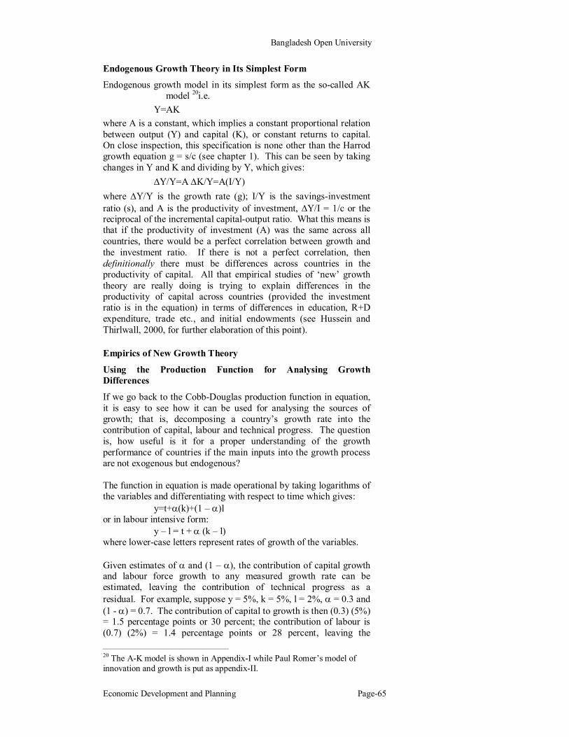
Bangladesh Open University
Economic Development and Planning Page-65
Endogenous Growth Theory in Its Simplest Form
Endogenous growth model in its simplest form as the so-called AK model 20i.e.
Y=AK where A is a constant, which implies a constant proportional relation between output (Y) and capital (K), or constant returns to capital. On close inspection, this specification is none other than the Harrod growth equation g = s/c (see chapter 1). This can be seen by taking changes in Y and K and dividing by Y, which gives:
Y/Y=A K/Y=A(I/Y) where Y/Y is the growth rate (g); I/Y is the savings-investment ratio (s), and A is the productivity of investment, Y/I = 1/c or the reciprocal of the incremental capital-output ratio. What this means is that if the productivity of investment (A) was the same across all countries, there would be a perfect correlation between growth and the investment ratio. If there is not a perfect correlation, then definitionally there must be differences across countries in the productivity of capital. All that empirical studies of ‘new’ growth theory are really doing is trying to explain differences in the productivity of capital across countries (provided the investment ratio is in the equation) in terms of differences in education, R+D expenditure, trade etc., and initial endowments (see Hussein and Thirlwall, 2000, for further elaboration of this point). Empirics of New Growth Theory
Using the Production Function for Analysing Growth Differences
If we go back to the Cobb-Douglas production function in equation, it is easy to see how it can be used for analysing the sources of growth; that is, decomposing a country’s growth rate into the contribution of capital, labour and technical progress. The question is, how useful is it for a proper understanding of the growth performance of countries if the main inputs into the growth process are not exogenous but endogenous? The function in equation is made operational by taking logarithms of the variables and differentiating with respect to time which gives:
y=t+(k)+(1 – )l or in labour intensive form:
y – l = t + (k – l) where lower-case letters represent rates of growth of the variables. Given estimates of and (1 – ), the contribution of capital growth and labour force growth to any measured growth rate can be estimated, leaving the contribution of technical progress as a residual. For example, suppose y = 5%, k = 5%, l = 2%, = 0.3 and (1 - ) = 0.7. The contribution of capital to growth is then (0.3) (5%) = 1.5 percentage points or 30 percent; the contribution of labour is (0.7) (2%) = 1.4 percentage points or 28 percent, leaving the 20 The A-K model is shown in Appendix-I while Paul Romer’s model of innovation and growth is put as appendix-II.

School of Business
Unit-2 Page-66
contribution of technical progress as 5% - 2.9% = 2.1% or 42 percent. Solow (1957) was the first to use the labour intensive form of the Cobb-Douglas production function in analysing the growth performance of the US economy over the previous fifty years, and concluded that only 10 percent of the growth of output per man could be ‘explained’ by the growth of capital per man leaving 90 percent of growth to be ‘explained’ by various forms of technical progress. Denison (1962, 1967) used the same production function approach, or growth accounting framework, to study growth performance in the US and between the countries of Europe, disaggregating the technical progress term (or residual) into various component parts. Maddison (1970) used the approach to study growth rate differences between developing countries. Since this early research, there has been a mass of other studies too extensive to survey here (but see Felipe, 1998), but two recent studies may be mentioned as illustrative. The World Bank (1991) did a study of 68 countries showing capital accumulation to be of prime importance, with technical progress minimal. This seems to be the central conclusion for developing countries in contrast to developed countries. Secondly, there is the controversial study by Alwyn Young (1995) of the four East Asian ‘dragons’ of Hong Kong, Singapore, South Korea and Taiwan which also shows that most of the growth in these countries can be explained by the growth of factor inputs and not technical progress, so that according to Young there has been no growth miracle in these countries – contrary to the conventional wisdom. Before accepting this conclusion, however, the observer still has to explain why there was such a rapid growth of factor inputs, and it is this point which exposes the fundamental weakness of the production function approach to the analysis of growth performance. On closer inspection, what distinguishes these countries is their outward orientation and relentless search for export markets, and their remarkable growth of exports which confers benefits on an economy from both the demand and supply side. This exposes another weakness of neoclassical growth theory and that is that the models are closed. There is no trade in these simple models, and no balance of payments to worry about. They are supply-oriented, supply-driven, closed economy models unsuitable for the analysis of open economies in which foreign exchange is invariably a scarce resource acting to constrain the growth process. Convergence The first crude test of new growth theory is to observe whether or not there is an inverse relation across countries between the growth of output per head and the initial level of per capita income of countries. If there is, this would be supportive of the neoclassical prediction of convergence. If not, it would be supportive of ‘new’ growth theory that the marginal product of capital does not decline. This is referred to as the test for beta () convergence. It can be said straight away that no global studies find evidence of unconditional beta convergence. Virtually all studies find evidence of divergence. The coefficient linking the growth of output per head to the initial level of per capita income is positive not negative.

Bangladesh Open University
Economic Development and Planning Page-67
Baumol (1986)21 examines convergence from 1870 to 1979 among the 16 industrialised countries for which Maddison (1982)22 provides data. Baumol regresses output growth over this period on a constant and initial income; that is, he estimates ln[ (Y/N) i, 1979 ] - ln[(Y/N)i ,1870] = a + b ln[(Y/N)i ,1870] + ε i Where ln(Y/N) is log income per person, ε is an error term, and i indexes countries. If there is convergence, b will be negative: countries with higher initial incomes have lower growth. The results are ln[ (Y/N) i, 1979 ] - ln[(Y/N)i ,1870] = 8.457 - 0.995 ln[(Y/N)i ,1870]
(0.994)
R2= 0.87, s.e.e = 0.15 Where the number in parentheses, 0.094, is the standard error of the regression coefficient De Long (1988)23 states that Baumol's findings are largely spurious. He finds out mainly two problems, the number one is sample selection and the other one is measurement error. For the first case he considers the richest countries as of 1870: more specifically, his sample consists of all countries at least as rich as the second poorest country in Baumol's sample in 1870. And for the second case he identifies that estimates of real income per capita in 1870 are imprecise. De Long formulates the following model: ln[ (Y/N) i, 1979 ] - ln[(Y/N)i ,1870]* = a + b ln[(Y/N)i ,1870]* + ε i ln[(Y/N)i ,1870] = ln[(Y/N)i ,1870]* + μ i Where ln[(Y/N)i ,1870]* is the true value of lof income per capita in 1870 and ln[(Y/N)i ,1870] is the measured value. ε and μ are assumed to uncorrelated with each other and with ln[(Y/N)i ,1870]*. Population Growth and Technological Change Kremer (1993)24 demonstrates that the hypothesis that growth arises from endogenous knowledge accumulation can be tested despite difficulties. He first notes that all models of the endogenous growth 21 Baumol, William. 1986. "Productivity of Growth , Convergence, and welfare." American Economic Review 76 (December): 1072- 1085. 22 Maddison, Angus. 1982. Phase of Capitalist Development. Oxford : Oxford University Press. 23 De Long, J. Bradford. 1988. "Productivity Growth, Convergence, and Welfare: Comment." American Economic Review 78 (December): 1138-1154. 24 Kremer, Micheal. 1993. "Population Growth and Technological Change: One Million B.C. to 1990." Quarterly Journal of Economics 108 (August): 681-716.

School of Business
Unit-2 Page-68
of knowledge predict that technological progress is an increasing function of population size. The reasoning is simple: the larger the population, the more people there are to make discoveries, and thus the more rapidly knowledge accumulates. Kremer's formal model is a straightforward variation on the models we have been considering. The simplest version consists of three equations. First, output depends on technology, labour, and land:
y(t) = Rα [A(t)L(t)]l-α,---------------------1
where R denotes the fixed stock of land. (Capital is neglected for simplicity, and land is included to keep population finite.) Second, the growth rate of knowledge is proportional to population:
A˚(t)/A(t) = BL(t) --------------------------2 And third, population adjusts so that output per person equals the subsistence level, denoted y/:
y(t)/L(t) = y/ -------------------3 To solve the model, begin by noting that (3) implies y(t) = y/L(t). Substituting this into (1) yields
y/L(t) = Rα[A(t)L(t)]l-α, -----------4 or
L(t) = [1/y/]1/α A(t)(l-α)/ α R. ---------------5
This equation states that the population that can be supported is decreasing in the subsistence level of output, increasing in technology, and proportional to the amount of land. Since y/ and R are constant the growth rate of L is (1- α)/ α times the growth rate of A. Expression 2 for the growth rate of A therefore implies
L˚(t)/L(t) = [(l-α)/ α][BL(t)]--------------- -6
Thus, in this simple form, the model implies not just that the growth rate of population is rising over time, but that it is proportional to the level of population.
Kremer tests this prediction by using population estimates extending back to 1 million B.C. that have been constructed by archaeologists and anthropologists. The following Figure shows the resulting scatterplot of population growth against population. Each observation shows the level of population at the beginning of some period and the average annual growth rate of population over that period. The length of the periods considered falls gradually from many thousand years early in the sample to 10 years at the end. Because the periods considered for the early part of the sample are so long, even substantial errors in the early population estimates would have little impact on the estimated growth rates. The figure shows a strongly positive, and approximately linear, relationship between population growth and the level of population. A regression of growth on a constant and population (in billions) yields nt = -0.0023 + 0.524 Lt, R2 = 0.92, D.W: = 1.10, -------7
(0.0355) (0.026)

Bangladesh Open University
Economic Development and Planning Page-69
where n is population growth and L is population, and where the numbers in parentheses are standard errors. Thus there is an overwhelmingly statistically significant association between the level of population and its growth rate.
The argument that technological progress is a worldwide phenomenon fails if there are regions that are completely cut off from one another. Kremer uses this observation to propose a second test of theories of endogenous knowledge accumulation. From the disappearance of the intercontinental land bridges at the end of the last ice age to the voyages of the European explorers, Eurasia-Africa, the Americas, Australia, and Tasmania were almost completely isolated from one another. The model implies that at the time of the separation, the populations of each region had the same technology; thus the initial populations should have been approximately proportional to the land areas of + + + + + + + + + + + + ++ + + Figure : The Level and Growth Rate of Population, 1 million B.C. to 1990. the regions (see equation [5]). The model predicts that during the period that the regions were separated, technological progress was faster in the regions with larger populations. The theory thus predicts that, when contact between the regions was re-established around 1500, population density was highest in the largest regions. Intuitively, inventions that would allow a given area to support more people, such as the domestication of animals and the development of agriculture, were much more likely in Eurasia-Africa, with its population of millions, than in Tasmania, with its population of a few thousand. The data confirm this prediction. The land areas of the four regions are 84 million square kilometers for Eurasia-Africa, 38 million for the Americas, 8 million for Australia, and 0.1 million for Tasmania. Population estimates for the four regions in 1500 imply densities of approximately 4.9 people per square kilometre for Eurasia-Africa, 0.4 for the Americas, and 0.03 for both Australia and Tasmania.
Popu
latio
n G
row
th R
ate
O 1 2 3 4 5 -0.005
-0.000
-0.010
-0.020
-0.025
Population (billions)

School of Business
Unit-2 Page-70
Physical and Human Capital Accumulation and Cross-Country Differences in Incomes When we allow for human capital we found that variations in population growth and capital accumulation have the potential to account for large cross-country differences in incomes. Mankiw, Romer, and Weil (1992) address the question of whether those variations in fact account for the differences. Mankiw, Romer, and Weil find that the estimated impact of saving and population growth on income is far larger than predicted by the Solow model with a capital share in the vicinity of one-third. Since the model with human capital predicts much larger impacts of saving and population growth on output than the Solow model does, this finding is encouraging for the human-capital model. Mankiw, Romer, and Weil's strategy is to estimate equation lny* = [α/(1- α -β] ln sk + [β/(1- α - β] ln sH -[( α + β /(1- α - β] In(n + g )-------------------- (8) As g is set to 0.05 for all countries, they measure sH as the average fraction of the population of working age that is in secondary school over the years 1960-1985. This is clearly an imperfect measure of the fraction of a country's resources devoted to human capital accumulation. Because sH enters in the equation logarithmically, if the true sH is proportional to this measure, only the constant term of the regression will be affected. Nonetheless, measurement error in sH is a concern. Rewriting slightly, the equation that Mankiw, Romer, and Weil estimate is lnyi = a + b[lnsKi -In(ni + 0.05)] + c[lnsRi -In(ni + 0.05)] + εi , ----9 where i indexes countries. The results for the broadest sample of countries are
lnyi = 7.86 + 0.73 [lnsKi -In(ni + 0.05)] + 0.67 [In ski -In(ni + 0.05)]-- 10
(0.14) (0.12) (0.07)
N = 98, R2 = 0.78, s.e.e. = 0.51, where the numbers in parentheses are standard errors. The values of α and β implied by these estimates of b and c (again with standard errors in parentheses) are α = 0.31 (0.04) and β = 0.28 (0.03). In addition, when In (ni + 0.05) is entered separately, its coefficient is approximately equal to minus the sum of the coefficients on ln sKi and In sHi, as the model predicts, and this restriction is not rejected statistically. Thus the model fits the data remarkably well: the implied shares of physical and human capital are reasonable, and the regression accounts for almost 80 percent of cross-country variation in output per worker.

Bangladesh Open University
Economic Development and Planning Page-71
A natural concern is that the saving rates, particularly sH, are endogenous: it may be that in countries that are wealthy for reasons not captured by the model, a larger fraction of the population is in school. But, as Mankiw, Romer, and Weil observe, this would cause upward bias in the estimate of β; the fact that the estimated β is if anything somewhat below direct estimates of human capital's share is therefore inconsistent with this possible explanation of the results. Mankiw, Romer and Weil then turn to the issue of convergence. They begin by noting that the model implies that countries with different levels of sK, sH, and n have different levels of output per worker on their balanced growth paths; thus there is a component of cross-country income differences that persists over time. But differences that arise because countries are initially at different points in relation to their balanced growth paths gradually disappear as the countries converge to those balanced growth paths. The model therefore predicts convergence controlling for the determinants of income on the balanced growth path, or conditional convergence. Specifically, one can show that the model implies that, in the vicinity of the balanced growth path, y converges to y* at rate (1- α –β (n + g) = λ
d ln y(t)/dt ≡ - λ[ln y(t) – ln y*]-------------------11 The above equation implies that lny approaches Iny* exponentially:
Iny(t) -Iny* ≡ e- λt[Iny(0) -Iny*]-------------------------------12
where y(0) is the value of y at some initial date. (By differentiating the above equation, it is straightforward to check that it implies that y(t) obeys (11). If α and β are each 1/3 and n + g is 6 percent, λ is 2 percent; this implies that a country moves halfway to its balanced growth path in 35 years. Adding In y* -In y (0) to both sides of (12) yields an expression for the growth of income:
Iny(t) -Iny(0) ≡ -(1 -e-λt )[Iny(0) -Iny*]. -------------------13 Note that (13) implies conditional convergence: countries with initial incomes that are low relative to their balanced growth paths have higher growth. Finally, using equation (8) to substitute for Iny* yields:
Iny(t) -Iny(0) ≡ (1- e-λt)Iny* -(1- e-λt)In y(0) = (1 -e-λt)[α/(1- α –β)][In sK –In (n + g)] + (1 - e-λt) [β /(1- α – β)][InsH -In(n + g)]-(1- e-λt )Iny(0).
Mankiw, Romer, and Weil estimate this equation, using the same data as before. The results are
Inyi(t) -Inyi(0) = 2.46 + 0.500 [lnsKi -In(ni + g)] (0.48) (0.082)

School of Business
Unit-2 Page-72
+ 0.238 [InsHi -In(ni + g)] -0.299 Inyi(0), ----------------14 (0.060) (0.061)
N = 98, R2 = 0.46, s.e.e. = 0.33.
The implied values of the parameters are α = 0.48 (0.07), β = 0.23 (0.05), and λ = 0.0142 (0.0019). The estimates are broadly in line with the predictions of the model: countries converge toward their balanced growth paths at about the rate that the model predicts, and the estimated capital shares are broadly similar to what direct evidence suggests. Overall, the evidence suggests that a model that maintains the assumption of diminishing returns to capital but that adopts a broader definition of capital than traditional physical capital, and therefore implies a total capital share closer to 1 than to 1/3 provides a good first approximation to the cross-country data. When it comes to interpreting the empirical results from testing models of new growth theory and convergence, some care needs to be taken. In particular, great care needs to be exercised in interpreting the negative sign on the initial level of per capita income as necessarily rehabilitating the neoclassical model of growth, as for example, Barro (1991) does, because there are other conceptually distinct reasons for expecting a negative sign. Firstly, outside the neoclassical paradigm, there is a whole body of literature that argues that economic growth should be inversely related to the initial level of per capita income because the more backward a country, the greater the scope for catch-up; that is, for absorbing a backlog of technology, which represents a shift in the whole production function. Is conditional convergence picking up diminishing returns to capital in the neoclassical sense, or catch-up? The two concepts are conceptually distinct, but not easy to disentangle empirically. Secondly, the negative term could simply be picking up structural change, with poor countries growing faster than rich countries (controlling for other variables) because of a more rapid shift of resources from low productivity to high productivity sectors (e.g. from agriculture to industry). How do we discriminate between these hypotheses? Critique The resurgence of interest in the theory of economic growth has, to quote Solow (1994), “an air of promise and excitement about it.” But the new theory has its share of shortcomings. Solow questions the simple characterisation in these models of the relation between investment in research and development – or what may be called “the knowledge sector” – on the one hand and production, on the other. He argues that there is probably “an irreducibly exogenous element” in the R&D process, hnec innovation can at best be partially endogenous (Solow, 1994).
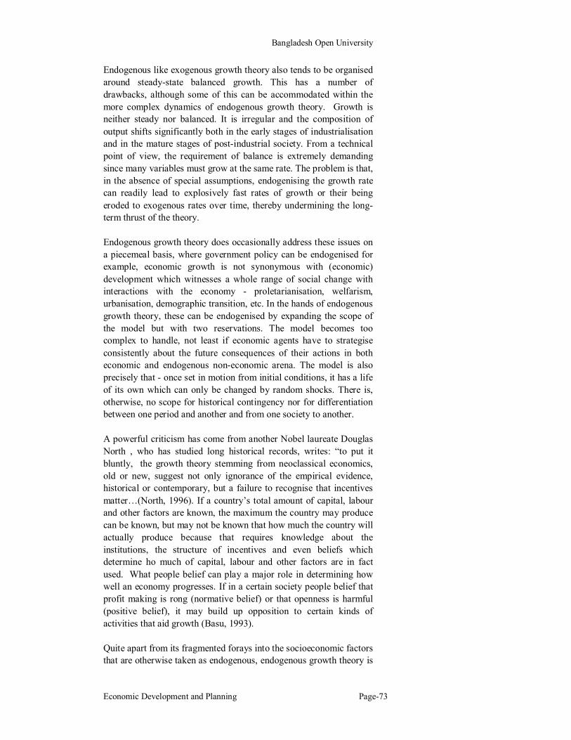
Bangladesh Open University
Economic Development and Planning Page-73
Endogenous like exogenous growth theory also tends to be organised around steady-state balanced growth. This has a number of drawbacks, although some of this can be accommodated within the more complex dynamics of endogenous growth theory. Growth is neither steady nor balanced. It is irregular and the composition of output shifts significantly both in the early stages of industrialisation and in the mature stages of post-industrial society. From a technical point of view, the requirement of balance is extremely demanding since many variables must grow at the same rate. The problem is that, in the absence of special assumptions, endogenising the growth rate can readily lead to explosively fast rates of growth or their being eroded to exogenous rates over time, thereby undermining the long-term thrust of the theory. Endogenous growth theory does occasionally address these issues on a piecemeal basis, where government policy can be endogenised for example, economic growth is not synonymous with (economic) development which witnesses a whole range of social change with interactions with the economy - proletarianisation, welfarism, urbanisation, demographic transition, etc. In the hands of endogenous growth theory, these can be endogenised by expanding the scope of the model but with two reservations. The model becomes too complex to handle, not least if economic agents have to strategise consistently about the future consequences of their actions in both economic and endogenous non-economic arena. The model is also precisely that - once set in motion from initial conditions, it has a life of its own which can only be changed by random shocks. There is, otherwise, no scope for historical contingency nor for differentiation between one period and another and from one society to another. A powerful criticism has come from another Nobel laureate Douglas North , who has studied long historical records, writes: “to put it bluntly, the growth theory stemming from neoclassical economics, old or new, suggest not only ignorance of the empirical evidence, historical or contemporary, but a failure to recognise that incentives matter…(North, 1996). If a country’s total amount of capital, labour and other factors are known, the maximum the country may produce can be known, but may not be known that how much the country will actually produce because that requires knowledge about the institutions, the structure of incentives and even beliefs which determine ho much of capital, labour and other factors are in fact used. What people belief can play a major role in determining how well an economy progresses. If in a certain society people belief that profit making is rong (normative belief) or that openness is harmful (positive belief), it may build up opposition to certain kinds of activities that aid growth (Basu, 1993). Quite apart from its fragmented forays into the socioeconomic factors that are otherwise taken as endogenous, endogenous growth theory is

School of Business
Unit-2 Page-74
built up on the basis of methodological individualism in which agents optimise or otherwise engage in activity according to more or less arbitrary behavioural patterns. Such an approach precludes the endogeneity of social forces, structures and relations, whether these be economic or otherwise, unless derived from aggregation over individuals. This is in sharp contrast to classical political economy with, for example, Smith's emphasis on the interaction between a growing division of labour within the constraints imposed by the extent of the market, and to Marx's theory of the accumulation of capital as the driving force behind productivity increase. In each of these cases, as for Ricardo's theory of differential rent, the value theory constructed is concerned to derive prices on the basis of a changing technology. How is value formed when technology is changing - whether it be due to growing division of labour, movement onto worse land, or the growing composition of capital. A significant continuity between exogenous and endogenous growth theory is that the latter incorporates shifting technology only on the basis of the same principle, even if more complex in practice - that of present value discounting of streams of utility.

Bangladesh Open University
Economic Development and Planning Page-75
Review Questions
Multiple Choice Questions 1. The Endogenous growth theories generally use neoclassical
model but allow the production function to exhibit: A. increasing returns to scale B. decreasing returns to scale C. diminishing returns to scale D. multiplier returns to scale
2. Solow used the ------------ form of the Cobb-Douglas production function in analysing the growth performance of the US economy.
A. capital intensive B. labour intensive C. knowledge intensive D. technology intensive
3. Kremer notes that all models of the endogenous growth of knowledge predict that technological progress is an increasing function of:
A. capital. B. human capital. C. population size. D. research and development.
4. Endogenous like exogenous growth theory also tends to be organised around:
A. steady-state unbalanced growth B. steady-state uneven growth C. steady-state biased growth D. steady-state balanced growth
Answers: 1. A; 2. B; 3. C and 4. D Short Questions
1. What rate the salient feature of AK model?
2. Make a distinction between AK and Romer (1990) model?
3. What does growth empirics suggest about endogenous growth theory?
Broad Questions
1. All models of the endogenous growth of knowledge predict that technological progress is an increasing function of population size – Explain.
2. Outline growth differences using the production function.
3. The first crude test of new growth theory is to observe whether or not there is an inverse relation across countries between the growth of output per head and the initial level of per capita income of countries – Explain and analyse the statement.
4. Discuss how cross-country differences in incomes can be captured through physical and human capital accumulation.

School of Business
Unit-2 Page-76
5. “Growth theory stemming from neoclassical economics, old or new, suggests...ignorance of the empirical evidence, historical or contemporary” – Analyse the statement.
6. Outline the AK model and discuss the source of economic growth.
7. Outline the model of endogenous innovation and growth and make a critical evaluation on the model.
8. “All models of the endogenous growth of knowledge predict that technological progress is an increasing function of population size,” – Explain.
Further Readings
1. Hayami ,Y. 1987. Development Economics. Clarendon Press. Oxford.
2. Kremer, Micheal. 1993. "Population Growth and Technological Change: One Million B.C. to 1990." Quarterly Journal of Economics 108 (August): 681-716.
3. Romer D, Advanced Macroeconomics, New York: McGrawhill, 1996.
4. Baumol, William. 1986. "Productivity of Growth , Convergence, and welfare." American Economic Review 76 (December): 1072- 1085.
5. Maddison, Angus. 1982. Phase of Capitalist Development. Oxford: Oxford University Press.
6. De Long, J. Bradford. 1988. "Productivity Growth, Convergence, and Welfare: Comment." American Economic Review 78 (December): 1138-1154.
7. Mankiw, N. Gregory. 1994. Macroeconomics. Second Edition. New York: Worth
8. Barro, Robert J., and Salai-I-Martin, Xavier. 1991."Convergence across states and regions". Brookings Paper on Economic Activity, no.1, 107-182.
9. Barro, Robert J., Mankiw, N. Gregory, and Salai-I-Martin, Xavier. 1995."Capital Mobility in Neoclassical Models of Growth ". American Economic Review 85 (March) : 103 -115.
10. Abramovitz (1956), Resource and Output Trends in the United States since 1870, American Economic Review Papers and Proceedings, May.
11. Arrow (1962), The Economic Implications of Learning by Doing, Review of Economic Studies, June.
12. R. Barro (1991), Economic Growth in a Cross Section of Countries, Quarterly Journal of Economics, May.
13. W. Baumol (1986), Productivity Growth, Convergence and Welfare, American Economic Review, December.
14. J. Cornwall (1977), Modern Capitalism: Its Growth and Transformation (London: Martin Robertson).
15. Denison (1962), The Sources of Economic Growth in the US and the Alternatives before Us, (New York: Committee for Economic Development, Library of Congress).

Bangladesh Open University
Economic Development and Planning Page-77
16. Denison (1967), Why Growth Rates Differ: Post-war Experience in Nine Western Countries (Washington DC: Brookings Institution).
17. Domar (1947), Expansion and Employment, American Economic Review, March.
18. Emmanuel (1972), Unequal Exchange: A Study of the Imperialism of Trade (New York: Monthly Review Press).
19. Esfahani (1991), Exports, Imports and Economic Growth in Semi-Industrialised Countries, Journal of Development Economics, January.
20. Feder (1983), On Exports and Economic Growth, Journal of Development Economics, February/April.
21. Felipe (1999), Total Factor Productivity Growth in East Asia: A Critical Survey, Journal of Development Studies, April.
22. Fingleton and J. McCombie (1996), Increasing Returns and Economic Growth: Some Evidence from the European Union Regions, Oxford Economic Papers, January
23. Frank (1967), Capitalism and Underdevelopment in Latin America (New York: Monthly Review Press).
24. Z. Griliches (1958), Research Costs and Social Returns: Hybrid Corn and Related Innovations, Journal of Political Economy, October.
25. Grossman and E. Helpman (1991), Innovation and Growth in the Global Economy (Cambridge, Mass: MIT Press).
26. J.D. Hansen and J. Zhang (1996), A Kaldorian Approach to Regional Economic Growth in China, Applied Economics, June.
27. R. Harrod (1933), International Economics (Cambridge: Cambridge University Press).
28. R. Harrod (1939), An Essay in Dynamic Theory, Economic Journal, March.
29. Hicks (1950), The Trade Cycle (Oxford: Clarendon Press). 30. Hirschman (1958), Strategy of Economic Development (New
Haven: Yale University Press). 31. Z.F. Hu and M.S. Khan (1997), Why is China Growing so
Fast?, IMF Staff Papers, March. 32. Hussein and A.P. Thirlwall (2000), The AK Model of ‘New’
Growth Theory is the Harrod-Domar Growth Equation: Investment and Growth Revisited, Journal of Post Keynsian Economics, Spring.
33. Journal of Post Keynesian Economics (1997), Symposium on Thirlwall’s Law, Spring.
34. Kaldor (1957), A Model of Economic Growth, Economic Journal, December.
35. Kaldor (1966), Causes of the Slow Rate of Economic Growth of the United Kingdom (Cambridge: Cambridge University Press).
36. Kaldor (1967), Strategic Factors in Economic Development (New York, Ithaca: New York State School of Industrial and Labour Relations, Cornell University).
37. Kaldor (1970), The Case for Regional Policies, Scottish Journal of Political Economy, November.

School of Business
Unit-2 Page-78
38. Kaldor (1972), ‘Advanced Technology in a Strategy for Development: Some Lessons from Britain’s Experience’, in Automation and Developing Countries (Geneva: ILO).
39. N. Kaldor (1985), Economics without Equilibrium (University College Cardiff Press).
40. N. Kaldor (1996), Causes of Growth and Stagnation in the World Economy (The Raffaele Lectures, Cambridge University Press).
41. J.M. Keynes (1937), Some Economic Consequences of a Declining Population, Eugenics Review, April.
42. Kindleberger (1967), Europe’s Postwar Growth: the Role of the Labour Supply (Cambridge, Mass: Harvard University Press).
43. Krugman (1989), Differences in Income Elasticities and Trends in Real Exchange Rates, European Economic Review, May.
44. Leibenstein (1957), Economic Backwardness and Economic Growth (New York: Wiley).
45. Leon-Ledesma (2000), Economic Growth and Verdoorn’s Law in the Spanish Regions 1962-91, International Review of Applied Economics, January.
46. Leon-Ledesma (2000), Accumulation, Innovation and Catching-Up: an Extended Cumulative Growth Model, Cambridge Journal of Economics.
47. Leon-Ledesma and A.P. Thirlwall (2001), The Endogeneity of the Natural Rate of Growth, Cambridge Journal of Economics,
48. Levine and D. Renelt (1992), A Sensitivity Analysis of Cross-Country Growth Regressions, American Economic Review, September.
49. Lewis (1954), Economic Development with Unlimited Supplies of Labour, Manchester School, May.
50. Lopez G. and A. Cruz B. (2000), “Thirlwall’s Law” and Beyond: the Latin American Experience, Journal of Post Keynesian Economics, Spring
51. Lucas (1988), On the Mechanics of Economic Development, Journal of Monetary Economics, Vol 22.
52. McCombie and A.P. Thirlwall (1994), Economic Growth and the Balance of Payments Constraint (London: Macmillan).
53. McCombie and J.R. de Ridder (1983), Increasing Returns, Productivity and Output Growth: The Case of the United States, Journal of Post Keynesian Economics, Spring
54. J. McCombie (1985), Increasing Returns and the Manufacturing Industries: Some Empirical Issues, The Manchester School, March
55. J. McCombie (1985), Economic Growth, the Harrod Foreign Trade Multiplier and the Hicks’ Super Multiplier, Applied Economics, February.
56. J. McCombie and A.P. Thirlwall (1997), The Dynamic Harrod Foreign Trade Multiplier and the Demand Oriented Approach to Economic Growth: An Evaluation, International Review of Applied Economics, January.

Bangladesh Open University
Economic Development and Planning Page-79
57. Maddison (1970), Economic Progress and Policy in Developing Countries (London: Allen and Unwin).
58. Malthus (1798), Essay on the Principle of Population (London: Penguin, 1983).
59. Marx (1867), Capital: A Critique of Political Economy, Vol.1 (New York: International Publishers, 1967).
60. T.R. Michl (1985), International Comparisons of Productivity Growth: Verdoorn’s Law Revisited, Journal of Post Keynesian Economics, Summer
61. J.C. Moreno-Brid (1999), Mexico’s Economic Growth and the Balance of Payments Constraint: A Cointegration Analysis, International Review of Applied Economics Vol.13 No 2.
62. J.C. Moreno-Brid (1998), Balance of Payments Constrained Economic Growth: The Case of Mexico, Banca Nazionale del Lavoro Quarterly Review, December.
63. G. Myrdal (1957), Economic Theory and Underdeveloped Regions (London: Duckworth).
64. R. Nelson (1956), A Theory of the Low Level Equilibrium Trap in Underdeveloped Countries, American Economic Review, December.
65. Nureldin-Hussain (1999), The Balance of Payments Constraint and Growth Rate Differences among African and East Asian Economies, African Development Review, June.
66. Okun (1962), Potential GNP: Its Measurement and Significance, Proceedings of the Business and Finance Statistics Section of the American Statistical Association.
67. R. Prebisch (1950), The Economic Development of Latin America and its Principal Problems (New York: ECLA, UN Dept. of Economic Affairs).
68. Ricardo (1817), Principles of Political Economy and Taxation (London: Everyman, 1992).
69. J. Robinson (1956), The Accumulation of Capital (London: Macmillan).
70. Romer (1986), Increasing Returns and Long Run Growth, Journal of Political Economy, October.
71. R. Sandilands (1990), Nicholas Kaldor’s Notes on Allyn Young’s LSE Lectures, 1927-29, Journal of Economic Studies, Vol.17 No 3/4/
72. T.W. Schultz (1961), Investment in Human Capital, American Economic Review, March.
73. Seers (1962), A Model of Comparative Rates of Growth of the World Economy, Economic Journal, March.
74. Smith (1776), An Inquiry into the Nature and Causes of the Wealth of Nations (London: Straham and Caddell).
75. R. Solow (1956), A Contribution to the Theory of Economic Growth, Quarterly Journal of Economics, February.
76. R. Solow (1957), Technical Change and the Aggregate Production Function, Review of Economics and Statistics, August.
77. R. Summers and A. Heston (1991), The Penn World Table (Mark 5): An Expanded Set of International Comparisons 1950-1966, Quarterly Journal of Economics, May.

School of Business
Unit-2 Page-80
78. Targetti and A.P. Thirlwall (1989), The Essential Kaldor (London: Duckworth).
79. A.P. Thirlwall (1969), Okun’s Law and the Natural Rate of Growth, Southern Economic Journal, July.
80. A.P. Thirlwall (1979), The Balance of Payments Constraint as an Explanation of International Growth Rate Differences, Banca Nazionale del Lavoro Quarterly Review, March.
81. A.P. Thirlwall (1983), Foreign Trade Elasticities in Centre-Periphery Models of Growth and Development, Banca Nazionale del Lavoro Quarterly Review, September.
82. A.P. Thirlwall (1986), A General Model of Growth and Development on Kaldorian Lines, Oxford Economic Papers, July.
83. A.P. Thirlwall (1987), Nicholas Kaldor (Brighton: Harvester Wheatsheaf Press).
84. A.P. Thirlwall (1987), Keynes and Economic Development (London: Macmillan).
85. A.P. Thirlwall and G. Sanna (1996), ‘”New” Growth Theory and the Macrodeterminants of Growth: An Evaluation and Further Evidence’ in P. Arestis (ed), Employment, Economic Growth and the Tyranny of the Market: Essays in Honour of Paul Davidson Vol.2 (Aldershot: Edward Elgar).
86. A.P. Thirlwall (1999), Growth and Development: with Special Reference to Developing Economies (London: Macmillan).
87. A.P. Thirlwall (2000), Trade Agreements, Trade Liberalisation and Economic Growth: A Selective Survey, African Development Review, December.
88. UNCTAD (1999), Trade and Development Report (Geneva: UNCTAD).
89. P.J. Verdoorn (1949), Fattori che Regolano lo Sviluppo della Produttivita del Lavoro, L’Industria, No 1. English translation by A.P. Thirlwall in L. Pasinetti (ed), Italian Economic Papers Vol II (Oxford University Press, 1993).
90. World Bank (1991), World Development Report (Washington: World Bank).
91. Allyn Young (1928), Increasing Returns and Economic Progress, Economic Journal, December.
92. Alwyn Young (1995), The Tyranny of Numbers: Confronting the Statistical Realities of the East Asian Growth Experience, Quarterly Journal of Economics, August.
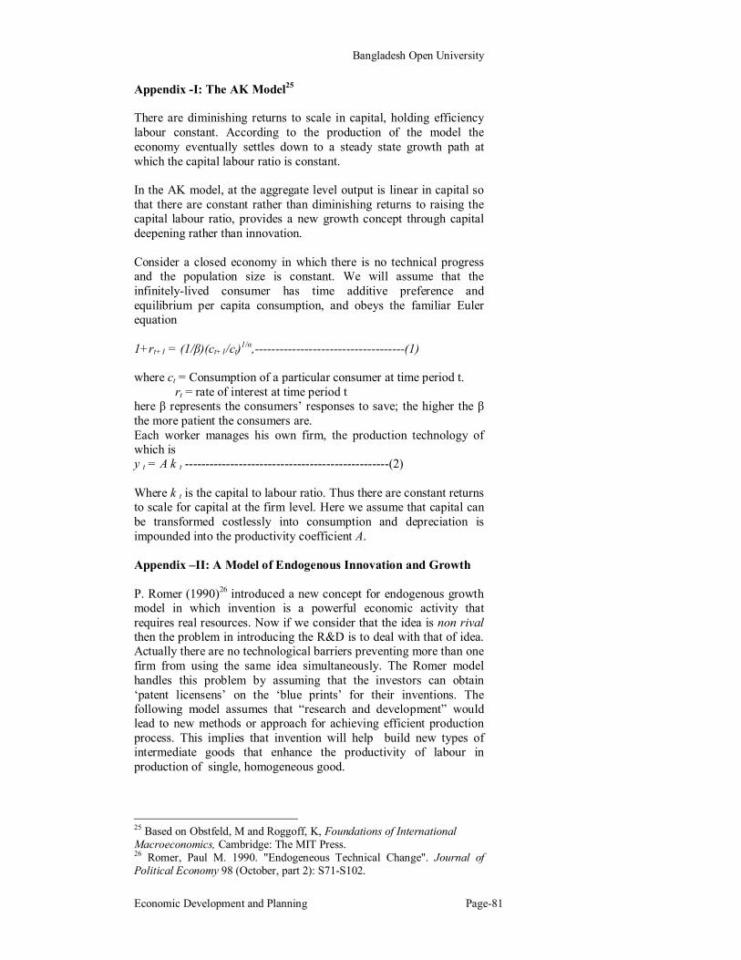
Bangladesh Open University
Economic Development and Planning Page-81
Appendix -I: The AK Model25 There are diminishing returns to scale in capital, holding efficiency labour constant. According to the production of the model the economy eventually settles down to a steady state growth path at which the capital labour ratio is constant. In the AK model, at the aggregate level output is linear in capital so that there are constant rather than diminishing returns to raising the capital labour ratio, provides a new growth concept through capital deepening rather than innovation. Consider a closed economy in which there is no technical progress and the population size is constant. We will assume that the infinitely-lived consumer has time additive preference and equilibrium per capita consumption, and obeys the familiar Euler equation 1+rt+1 = (1/β)(ct+1/ct)1/α,------------------------------------(1) where ct = Consumption of a particular consumer at time period t. rt = rate of interest at time period t here β represents the consumers’ responses to save; the higher the β the more patient the consumers are. Each worker manages his own firm, the production technology of which is y t = A k t -------------------------------------------------(2) Where k t is the capital to labour ratio. Thus there are constant returns to scale for capital at the firm level. Here we assume that capital can be transformed costlessly into consumption and depreciation is impounded into the productivity coefficient A. Appendix –II: A Model of Endogenous Innovation and Growth P. Romer (1990)26 introduced a new concept for endogenous growth model in which invention is a powerful economic activity that requires real resources. Now if we consider that the idea is non rival then the problem in introducing the R&D is to deal with that of idea. Actually there are no technological barriers preventing more than one firm from using the same idea simultaneously. The Romer model handles this problem by assuming that the investors can obtain ‘patent licensens’ on the ‘blue prints’ for their inventions. The following model assumes that “research and development” would lead to new methods or approach for achieving efficient production process. This implies that invention will help build new types of intermediate goods that enhance the productivity of labour in production of single, homogeneous good.
25 Based on Obstfeld, M and Roggoff, K, Foundations of International Macroeconomics, Cambridge: The MIT Press. 26 Romer, Paul M. 1990. "Endogeneous Technical Change". Journal of Political Economy 98 (October, part 2): S71-S102.

School of Business
Unit-2 Page-82
The whole production process is segmented: Final Goods Production Consider a closed economy in which the ‘Final Goods Production Function” is given below
At yt = Ly,t
1-α ∑ kj,tα
-------------------------------------------------------------(1)
j=1 Here, j = 1,2,………….. At implies the different types of capital goods kj. The parameter At shows the number of types of capital that has been invented at time t. Ly denotes the labour engaged in the production of final good. Romer actually used this human capital as a third factor, for simplicity we used labour in this manner. The economy’s total labour supply is L In this equation the production function is additively separable function of the different types of capital goods that implies an increase in the kj does not have any effect on ki. dy/dk = α Ly
1-α kJα-1----------------------------------------------------(2)
Equation (2) is independent of the level of all other capital goods. This also shows that there are decreasing type of investment for any capital in use; but the marginal product of any new capital will be α Ly
1-α kJα-1
k j = 0 = ∞----------------------------------------------(3) Production Blue prints A blue print shows how to combine raw material to produce quantities of the new capital good. One unit of final good input t yields one unit of kj,t+1. Assume that a blueprint can be put into the production immediately after the period it is developed, and that capital goods produced in period t would depreciate by 100% when it is used in the next period. It is also assumed that production in the R&D sector depends on the labour employed LA and on the current technology. At+1- At= θ At LA,t-----------------------------------------------(4) Here θ is a productivity shift parameter. We assume that total labour force is constant, labour is available for only R&D sector and final goods production. L= LA+Ly-------------------------------------------------- (5) From the equation (4) we will get two important insights: the greater the lengths of the existing knowledge the lower the labour cost of generating knowledge, the other one implies that there are constant returns to scale in A alone. Our main aim is to get what percents of labour is employed in the R&D sector and how final output is divided between investment and consumption. Let us first tackle the pricing system. Pricing System and Production of Intermediate goods Assume that firms in the R&D sector sell blueprints to the intermediate sector that manufactures the design in period t, again machines will be sold to the final good sector for the use in the period in t+1. Once an intermediate good producer buys the blueprint to produce capital good j, it will become the monopoly supplier of that type of capital goods to the final goods sector.
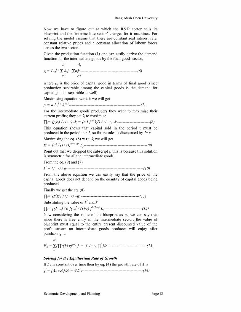
Bangladesh Open University
Economic Development and Planning Page-83
Now we have to figure out at which the R&D sector sells its blueprint and the ‘intermediate sector’ charges for it machines. For solving the model assume that there are constant real interest rate, constant relative prices and a constant allocation of labour forces across the two sectors. Given the production function (1) one can easily derive the demand function for the intermediate goods by the final goods sector,
At At yt = Ly,t
1-α ∑ kj,tα
- ∑pjkj------------------------------------------(6) j=1 j=1 where pj is the price of capital good in terms of final good (since production separable among the capital goods kj the demand for capital good is separable as well) Maximising equation w.r.t. kj we will get pj = α Ly
1-α kJα-1-----------------------------------------------------(7)
For the intermediate goods producers they want to maximise their current profits; they set kj to maximise ∏j = (pjkj) / (1+r) -kj = (α Ly
1-α kJα) / (1+r) -kj------------------------(8)
This equation shows that capital sold in the period t must be produced in the period in t-1, so future sales is discounted by 1+r. Maximising the eq. (8) w.r.t. kj we will get K/ = [α2 / (1+r)]1/(1- α) Ly-----------------------------------------------(9) Point out that we dropped the subscript j, this is because this solution is symmetric for all the intermediate goods. From the eq. (9) and (7) P/ = (1+r) / α---------------------------------------------------------(10) From the above equation we can easily say that the price of the capital goods does not depend on the quantity of capital goods being produced. Finally we get the eq. (8) ∏j = (P/K/) / (1+r) –K/ -------------------------------------------(11) Substituting the value of P/ and k/ ∏j = [(1- α) / α ][ α2 / (1+r) ]1/(1- α) Ly----------------------------(12) Now considering the value of the blueprint as pA we can say that since there is free entry in the intermediate sector, the value of blueprint must equal to the entire present discounted value of the profit stream an intermediate goods producer will enjoy after purchasing it. ∞ P/
A = ∑[∏//(1+r)(s-t) ] = [(1+r) ∏/ ]/r -----------------------------(13) s=t Solving for the Equilibrium Rate of Growth If LA is constant over time then by eq. (4) the growth rate of A is g/ = [At+1-At]/At = θ L/
A---------------------------------------------(14)

School of Business
Unit-2 Page-84
From equation (14) and (15) we will get a technology-determined relationship between the rate of growth of the economy and the rate of interest.27 g/ = θ L – r/ α ------------------------------------------------------(15) Expressing this in terms of gross interest rate the growth rate becomes 1+g/ = [θ L + (1+ α)/ α] –(1+r)/ α --------------------------------(16) It is expected that this is downward sloping as mentioned by the XX/ curve in the figure.
Figure1: Paul Romer’s growth model From eq. (9) of the previous lesson we can write [β (1+rt+1 )] α = (ct+1/ct) = 1+ g/
1+r = (1/ β) (1+g)1/α-------------------------------------(17) Eq. (17) is illustrated in the figure 1 as upward sloping curve. Since we have already assumed that capital depreciate by 100% the economy easily jumps to steady state in which K,Y,C , a grows at the constant rate. Here the points should be noted down that Endogenous Growth theory has evolved on the basis of two complementary impulses. The first one is to model the sources of productivity increase in various ways. Apart from technological spill-overs or learning by doing which arise spontaneously out of accumulation itself, productivity increase has been modelled by focusing upon the different stages in
27 If we want to determine the supply side of the model we have to find out the allocation of the human capital between the R&D sector and the final goods sector. Equating the marginal product of labour in the two sectors we can easily get the labour employed in the final sector; from this eq. (50) can be derived.
Gross rate of growth, 1=g
Gross real interest rate, 1+r 1+r
1+g/
1+ r/
X
X/
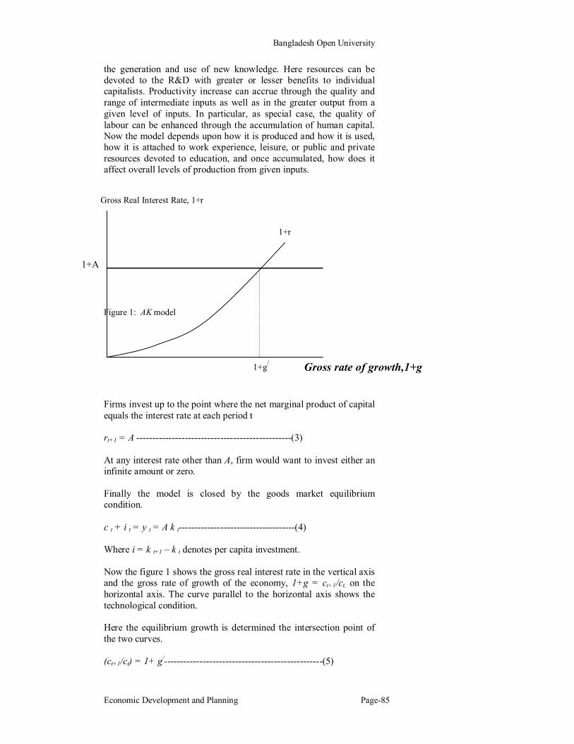
Bangladesh Open University
Economic Development and Planning Page-85
the generation and use of new knowledge. Here resources can be devoted to the R&D with greater or lesser benefits to individual capitalists. Productivity increase can accrue through the quality and range of intermediate inputs as well as in the greater output from a given level of inputs. In particular, as special case, the quality of labour can be enhanced through the accumulation of human capital. Now the model depends upon how it is produced and how it is used, how it is attached to work experience, leisure, or public and private resources devoted to education, and once accumulated, how does it affect overall levels of production from given inputs. Figure 1: AK model Firms invest up to the point where the net marginal product of capital equals the interest rate at each period t rt+1 = A ------------------------------------------------(3) At any interest rate other than A, firm would want to invest either an infinite amount or zero. Finally the model is closed by the goods market equilibrium condition. c t + i t = y t = A k t------------------------------------(4) Where i = k t+1 – k t denotes per capita investment. Now the figure 1 shows the gross real interest rate in the vertical axis and the gross rate of growth of the economy, 1+g = ct+1/ct, on the horizontal axis. The curve parallel to the horizontal axis shows the technological condition. Here the equilibrium growth is determined the intersection point of the two curves. (ct+1/ct) = 1+ g/-------------------------------------------------(5)
Gross Real Interest Rate, 1+r
1+r
1+A
1+g/ Gross rate of growth,1+g

School of Business
Unit-2 Page-86
The main difference between this model and the neo-classical growth model is that a change in the saving rate has now permanent effect on the growth rate. And market outcome of this model is Pareto optimal.
Lets consider the “Learning by doing” variant of the model. In this case each firm j’s output is given by
yjt = A ( kj
t ) α kt 1-α------------------------------------------(6)
Where k j is the individual firm’s level of capita per worker, and k is the economy wide average level of capital per worker. Arrow (1962)28 first proposed this variant and the rational for this is that the production process generates knowledge externalities. For example, Arrow cites the empirical regularity that after a new airplane design is introduced, the time required to build the frame of a marginal aircraft is inversely proportional to the cube root of the number of aircraft of that model that have already been produced; this improvement in productivity occurs without any evident innovations in the production process. Thus the accumulation of Knowledge occurs in part not as a result of deliberate efforts, but as a side effect of conventional economic activity. This type of knowledge accumulation is known as Learning by doing [ Romer (1996)]29
Here the higher the average levels of capital intensity the greater the incidence of technological spillovers that raise the marginal productivity of capital throughout the economy.
So, an individual expects the marginal product of its own investment as dyj/dkj = α A (k/kj)1- α--------------------------------------------(7)
Figure 2: Learning by doing in the AK model.
28 Arrow,Kenneth J. 1962. "The Economic Implications of Learning by Doing". Review of Economic Studies 29 (June): 155 - 173. 29 Romer David, 1996. Advanced Macro economics. Mcgraw-Hill
Market Solution
Social Optimum
1+r
Gross Real Interest Rate, 1+r
1+ A
1+αA
1+g/ Gross Rate of Growth, 1+g