The University of AkronIdeaExchange@UAkron

Honors Research Projects The Dr. Gary B. and Pamela S. Williams HonorsCollege

Spring 2016

Zipping Towards STEM: Simulation Wind TunnelEmma Piersonelp22@zips.uakron.edu

Greg Flohr

Devon Goldberg

Brandon Hein

Jeremy Hein

Please take a moment to share how this work helps you through this survey. Your feedback will beimportant as we plan further development of our repository.Follow this and additional works at: http://ideaexchange.uakron.edu/honors_research_projects

Part of the Aerospace Engineering Commons, and the Mechanical Engineering Commons

This Honors Research Project is brought to you for free and open access by The Dr. Gary B. and Pamela S. WilliamsHonors College at IdeaExchange@UAkron, the institutional repository of The University of Akron in Akron, Ohio,USA. It has been accepted for inclusion in Honors Research Projects by an authorized administrator ofIdeaExchange@UAkron. For more information, please contact mjon@uakron.edu, uapress@uakron.edu.

Recommended CitationPierson, Emma; Flohr, Greg; Goldberg, Devon; Hein, Brandon; and Hein, Jeremy, "Zipping Towards STEM:Simulation Wind Tunnel" (2016). Honors Research Projects. 391.http://ideaexchange.uakron.edu/honors_research_projects/391

Zipping Towards STEM: Simulation Wind

Tunnel

Senior Design Project Fall 2015/Spring 2016

Emma Pierson

Team Members:

Greg Flohr

Devon Goldberg

Brandon Hein

Jeremy Hein

Emma Pierson

Table of Contents

Introduction ................................................................................................................. 1

Graphical User Interface Design & Functionality ……………………………………. 1

Computational Fluid Dynamics & Program Outputs ………………………………… 4

2D CFD Method ................................................................................................. 6

3D CFD Method ................................................................................................. 9

Importing Figures ……………………………………………………………... 12

Hole Finder Function …………………………………………………………. 13

CFD Outputs …………………………………………………………………... 14

Drag Calculations ……………………………………………………………... 16

Buchtel Community Learning Center Trial ………….……………………………….. 19

Conclusion …...………………………………………………………………………... 20

References ……………..…………………………………………………………….. 21

Nomenclature

Symbol Description U Velocity in x-direction

V Velocity in y-direction

W Velocity in z-direction

p pressure

x x-direction, length of wind tunnel

y y-direction, height of wind tunnel

z z-direction, depth of wind tunnel

* Indicates first intermediate velocity

** Indicates second intermediate velocity

Uh U velocity averaged in the x-direction

Uv U velocity averaged in the y-direction

Uw U velocity averaged in the z-direction

�̃�ℎ U velocity difference in the x-direction

�̃�𝑣 U velocity difference in the y-direction

�̃�𝑤 U velocity difference in the z-direction

Vh V velocity averaged in the x-direction

Vv V velocity averaged in the y-direction

Vw V velocity averaged in the z-direction

�̃�ℎ V velocity difference in the x-direction

�̃�𝑣 V velocity difference in the y-direction

�̃�𝑤 V velocity difference in the z-direction

Wh W velocity averaged in the x-direction

Wv W velocity averaged in the y-direction

Ww W velocity averaged in the z-direction

�̃�ℎ W velocity difference in the x-direction

�̃�𝑣 W velocity difference in the y-direction

�̃�𝑤 W velocity difference in the z-direction

Re Reynolds number

∆t Change in time

P Pressure

n Indicates current time step

n+1 Indicates next time step

∇ Divergence

∆ Laplace

β Pressure Poisson stability term

τw Shear

hx Grid density in x-direction

hy Grid density in y-direction

hz Grid density in z-direction

1

Introduction The simulation wind tunnel program created for this project is implemented within a larger,

National Science Foundation funded project titled Zipping Towards STEM: Integrating

Engineering Design into the Middle School Physical Science Curriculum. Over the course of the

next two years, all Akron Public School 8th grade students will go through the Zipping Towards

STEM project curriculum. The students will be exposed to the typical steps of engineering design

(computer modeling, simulation, building, and testing) and learn about the fundamentals of

aerodynamics through the design of their own Soap Box Derby mini-cars. The virtual wind tunnel

will be used during the simulation portion of the curriculum to show the 8th grade students how

performance prediction software is used during the engineering design process.

Graphical User Interface Design & Functionality The graphical user interface (GUI) for the virtual wind tunnel was built using the Graphical

User Interface Development Environment (GUIDE) available in MATLAB. The functionality

available through GUIDE provided the team with the ability to package the wind tunnel program

in a user-friendly graphical interface. The interface that the students first see upon opening the

wind tunnel program can be seen in Figure 1.

Figure 1: Initial View of Simulation Wind Tunnel Program

2

The students are able to view the velocity profile, streamlines, pressure map, and drag of

predetermined 2D figures. With the 2D button selected, the students can access the list of 2D

shapes through the ‘Basic Shapes’ menu tab. The list of 2D shapes includes wedge, semicircle,

box, trapezoid, rectangle, and the side profile of a car. Students also have the option to choose

whether they want the analysis to show streamlines, pressure map, or both. The analysis that

students see on a simple box shape can be seen in Figure 2.

Figure 2: 2D Simple Shape “Box” Analysis

The students have the option to choose a simulation velocity between 1 and 40 mph, and they are

also able to scale the chosen 2D figure to a bigger or smaller size. The final streamline, pressure

map, and drag force results as viewed by the students can be seen in Figure 2. A color scale also

appears at the end of the analysis so that the students can interpret the high and low pressure areas

of the pressure map.

After the middle school students use the 2D functionality of the simulation wind tunnel to

learn about the aerodynamics of different shapes, they are also able to design their own Soap Box

Derby mini car. The students are encouraged to create a car design which they believe is

aerodynamically sound. The students are then able to import the stereolithography (.stl) file format

3

of their car design into the wind tunnel to view the predicted drag force of the design. An .stl file

uploaded into the software is shown in Figure 3.

Figure 3: Imported 3D Figure

The students are able to orient their car using the rotate (x, y, and z) buttons so that the front of the

car faces the inlet of the wind tunnel (denoted by a blue arrow in the GUI when the figure is

imported). Once the students have their car design set up to run correctly, they push the “run

analysis” button to view the computational analysis. The main window of the simulation software

after analysis is shown in Figure 4.

Figure 4: Main Window of Simulation Software, 3D Analysis

4

The 3D functionality still allows the students to specify a velocity between 1 and 40 mph, and then

view the predicted drag force. There is also be a pop-up window through which the students can

rotate their view to see all 3D aspects of the analysis and how the wind is moving around the car

from different angles. This can be seen in Figure 5.

Figure 5: Pop-Up Window of Simulation Software, 3D Analysis

After the students use the simulation software, they have the opportunity to redesign their soap

box derby car. After a final design is decided upon, the car designs are 3D printed and tested in

an actual wind tunnel. Finally, the students have a chance to compete against other students with

their designs on a race track.

Computational Fluid Dynamics & Program Outputs

Computational fluid dynamics, or CFD, is the numerical analysis of problems that involve

the flow of fluid in a given domain. There are many CFD programs that are on the market today,

but they are all expensive and too difficult for 8th graders to use. Also, these CFD software

programs are meant for very precise applications and sometimes require extremely long run times

to complete an analysis. For this project, the objective is to design a software that will run fast so

5

the students will not get distracted while it is running. This also means that accuracy is sacrificed,

which is acceptable given the students are just designing mini soap box cars.

Before a code could be written for our software, it was important to understand how CFD

codes work. First, a domain must be defined. For this virtual wind tunnel, the domain was defined

as the same space that is in the actual wind tunnels the students will use. Next, this domain needs

to be split up into a grid for computing. There are two options when selecting a grid for the domain.

They are a structured grid and an unstructured grid. It was decided that a structured grid would be

the best choice because an unstructured grid is complicated to create and makes the computations

more complicated. Then, boundary conditions need to be defined for the domain, like inlets, outlets

and walls where fluid cannot pass through.

Figure 6: Boundary Conditions Used for Wind Tunnel Domain

Finally, the Navier Stokes equations need to be numerically approximated across the

domain to give an approximation of what is actually happening inside the wind tunnel. When these

approximations are done, the velocity and pressure of the fluid is known in the entire domain. The

Navier Stokes equations are a set of partial differential equations that govern viscous flow. Because

these set of equations are partial differential equations it is very difficult to approximate a solution

to them. After completing research, a simple CFD code that simulated 2D lid driven cavity flow

was found from a paper written by Benjamin Seibold [1]. This code used a structured grid and was

6

able to successfully able to approximate a solution to the Navier Stokes equations quickly, which

is exactly what was needed.

Two Dimensional CFD Method

Before the method in this paper is described, the 2D incompressible Navier Stokes

equations need to be defined [2]:

𝜕𝑢

𝜕𝑡+

𝜕𝑢2

𝜕𝑥+

𝜕𝑢𝑣

𝜕𝑦= −

𝜕𝑃

𝜕𝑥+

1

𝑅𝑒(

𝜕𝜏𝑥𝑥

𝜕𝑥+

𝜕𝜏𝑥𝑦

𝜕𝑦)

(1)

𝜕𝑣

𝜕𝑡+

𝜕𝑢𝑣

𝜕𝑥+

𝜕𝑣2

𝜕𝑦= −

𝜕𝑃

𝜕𝑥+

1

𝑅𝑒(

𝜕𝜏𝑥𝑦

𝜕𝑥+

𝜕𝜏𝑦𝑦

𝜕𝑦)

(2)

𝜕𝑢

𝜕𝑥+

𝜕𝑣

𝜕𝑦= 0

(3)

where equations 1 and 2 are the momentum equations and equation 3 is the continuity equation.

The code uses a three step projection method of approximating these equations. This three step

method splits up the Navier Stokes equations into three sections that need to be solved for each

time step: nonlinear terms, viscous terms, and pressure correction. In the following equations that

describe how each section was solved, the capital letters, U and V, will be the approximations of

the actual velocity field. We will also assume that Un and Vn are the components of velocity at the

nth time step. Any U or V with an asterisk is an intermediate velocity component that needs to be

solved to find the next time step of n+1. In each section defined, an intermediate velocity field will

be solved for and then passed down to the following section. The flow chart below shows which

velocity terms are solved for and what section they passed to.

7

U*, V* U**,V** Un+1,Vn+1

Nonlinear Terms Viscous Terms Pressure Correction

Figure 7: Intermediate Velocity Field Flow Chart

The first section of this method from the Seibold paper is solving the nonlinear terms. The

nonlinear terms were treated explicitly and a linear combination of upwinding and the central

difference method was used to solve. Below is the method to approximate the nonlinear terms with

just the central differencing method:

𝑈∗ − 𝑈

∆𝑡= −

𝜕(𝑈ℎ)2

𝜕𝑥−

𝜕(𝑈𝑣𝑉ℎ)

𝜕𝑦

(4)

𝑉∗ − 𝑉

∆𝑡= −

𝜕(𝑉𝑣)2

𝜕𝑦−

𝜕(𝑈𝑣𝑉ℎ)

𝜕𝑥

(5)

With this, equations 4 and 5 were combined with the upwinding method to give the final

approximations of the nonlinear terms with the linear combination of the upwinding method and

central differencing method:

𝑈∗ − 𝑈

∆𝑡= −

𝜕((𝑈ℎ)2 − 𝛾|𝑈ℎ|�̃�ℎ)

𝜕𝑥−

𝜕(𝑈𝑣𝑉ℎ − 𝛾|𝑉ℎ|�̃�𝑣)

𝜕𝑦

(6)

𝑉∗ − 𝑉

∆𝑡= −

𝜕(𝑈𝑣𝑉ℎ − 𝛾|𝑈𝑣|�̃�ℎ)

𝜕𝑥−

𝜕((𝑉𝑣)2 − 𝛾|𝑉𝑣|�̃�𝑣)

𝜕𝑦

(7)

Where U* and V* are the intermediate velocities that are solved for in the code and then passed

down to the viscous terms. The tilde in these equations signify that the difference in the direction

indicated by the superscript of that term was taken. Also, gamma in equations 6 and 7 acts as the

transition parameter between central differencing and upwinding. The equation for this variable

can be seen in the code.

The next section is the viscous terms. These terms were treated implicitly, which means

that there would be two linear systems that needed to be solved every time step.

8

𝑈∗∗ − 𝑈∗

∆𝑡=

1

𝑅𝑒(

𝜕2𝑈∗∗

𝜕𝑥2+

𝜕2𝑈∗∗

𝜕𝑦2)

(8)

𝑉∗∗ − 𝑉∗

∆𝑡=

1

𝑅𝑒(

𝜕2𝑉∗∗

𝜕𝑥2+

𝜕2𝑉∗∗

𝜕𝑦2)

(9)

Here, U** and V** are the intermediate velocity terms that need to be solved for and then passed

down to the pressure correction section. In the code, this is done by using elimination with

reordering to compute the inverse matrices exactly by using the sparse Cholesky decomposition

[1].

The last step for solving for the velocity field is pressure correction. During this last step

the pressure is solved for and the velocity field is updated based on pressure differences in the

domain. To find pressure, it was treated implicitly and we can use the following vector equation:

−∆𝑃𝑛+1 = −

1

∆𝑡𝛻 ⋅ 𝑈𝑛

(10)

Where pressure will need to be solved for at each time step. So, solving this equation and finding

pressure can be done in the following four steps (reminder: all equations in these steps are in vector

form).

1. Compute the divergence of Un, 𝐹𝑛 = 𝛻 ⋅ 𝑈𝑛

2. Solve the pressure Poisson equation to find pressure field, −∆𝑃𝑛+1 = −1

∆𝑡𝐹𝑛

3. Compute the difference of pressure in all directions, 𝐺𝑛+1 = 𝛻𝑃𝑛+1

4. Update velocity field, 𝑈𝑛+1 = 𝑈𝑛 − ∆𝑡𝐺𝑛+1

It is important to remember that Un in the above steps is actually U** and V** that was solved for

in the viscous terms, and Un+1 is the velocity field in the next time step. Steps 1, 3, and 4 can all

be done easily. The second step is solved just as the implicit viscous terms were solved as described

above.

9

After completing the pressure correction step and finding the velocity field, Un+1, these

three sections are iterated through by feeding Un+1 back into the nonlinear terms, equations 6 and

7, and repeating the process. There is no convergence criteria set for this code, so it will not stop

running until the final time set by the user is reached.

Three Dimensional CFD Method

Since the objective of this project is to have the capability of importing 3D CAD

drawings, the above method for solving the 2D incompressible Navier Stokes equations needed to

be modified. First, the 3D incompressible Navier Stokes equations are defined [2]:

𝜕𝑢

𝜕𝑡+

𝜕𝑢2

𝜕𝑥+

𝜕𝑢𝑣

𝜕𝑦+

𝜕𝑢𝑤

𝜕𝑧= −

𝜕𝑃

𝜕𝑥+

1

𝑅𝑒(

𝜕𝜏𝑥𝑥

𝜕𝑥+

𝜕𝜏𝑥𝑦

𝜕𝑦+

𝜕𝜏𝑥𝑧

𝜕𝑧)

(11)

𝜕𝑣

𝜕𝑡+

𝜕𝑢𝑣

𝜕𝑥+

𝜕𝑣2

𝜕𝑦+

𝜕𝑣𝑤

𝜕𝑧= −

𝜕𝑃

𝜕𝑥+

1

𝑅𝑒(

𝜕𝜏𝑥𝑦

𝜕𝑥+

𝜕𝜏𝑦𝑦

𝜕𝑦+

𝜕𝜏𝑦𝑧

𝜕𝑧)

(12)

𝜕𝑤

𝜕𝑡+

𝜕𝑢𝑤

𝜕𝑥+

𝜕𝑣𝑤

𝜕𝑦+

𝜕𝑤2

𝜕𝑧= −

𝜕𝑃

𝜕𝑥+

1

𝑅𝑒(

𝜕𝜏𝑥𝑧

𝜕𝑥+

𝜕𝜏𝑦𝑧

𝜕𝑦+

𝜕𝜏𝑧𝑧

𝜕𝑧)

(13)

𝜕𝑢

𝜕𝑥+

𝜕𝑣

𝜕𝑦+

𝜕𝑤

𝜕𝑧= 0

(14)

These equations are very similar to equations 1, 2, and 3, where the only difference is the addition

of the third dimension in all equations and an addition of a third momentum equation. The method

for approximating the solution to these equations will be exactly the same as the method described

the Siebold paper for the 2D equations in some sections and slightly different in others. The 3D

code still uses a three section method, just as 2D, by splitting up nonlinear terms, viscous terms

and pressure correction.

First is solving for the nonlinear terms. For this section it was possible to copy the exact

method used for the 2D code. The only change that needed to be done was to update equations 6

10

and 7 to 3D equations. The equation for the linear combination of central differencing and

upwinding for the 3D nonlinear terms were:

𝑈∗ − 𝑈

∆𝑡= −

𝜕((𝑈ℎ)2 − 𝛾|𝑈ℎ|�̃�ℎ)

𝜕𝑥−

𝜕(𝑈𝑣𝑉ℎ − 𝛾|𝑉ℎ|�̃�𝑣)

𝜕𝑦−

𝜕(𝑈𝑤𝑊ℎ − 𝛾|𝑊ℎ|�̃�𝑤)

𝜕𝑧

(15)

𝑉∗ − 𝑉

∆𝑡= −

𝜕(𝑈𝑣𝑉ℎ − 𝛾|𝑈𝑣|�̃�ℎ)

𝜕𝑥−

𝜕((𝑉𝑣)2 − 𝛾|𝑉𝑣|�̃�𝑣)

𝜕𝑦−

𝜕(𝑉𝑤𝑊𝑣 − 𝛾|𝑊𝑣|�̃�𝑤)

𝜕𝑧

(16)

𝑊∗ − 𝑊

∆𝑡= −

𝜕(𝑈𝑤𝑊ℎ − 𝛾|𝑈𝑤|�̃�ℎ)

𝜕𝑥−

𝜕(𝑉𝑤𝑊𝑣 − 𝛾|𝑉ℎ|�̃�𝑣)

𝜕𝑦

−𝜕((𝑊𝑤)2 − 𝛾|𝑊𝑤|�̃�𝑤)

𝜕𝑧

(17)

As before, the velocity components, U*, V*, and W* are what is being solved for and then will be

passed down to the viscous terms. The w superscript in these three equations indicate that the term

was averaged across the width of the domain.

Next, the method for solving the viscous terms was modified. These terms were still treated

implicitly which gave three linear systems that needed to be solved every time step.

𝑈∗∗ − 𝑈∗

∆𝑡=

1

𝑅𝑒(

𝜕𝑈∗∗

𝜕𝑥+

𝜕𝑈∗∗

𝜕𝑦+

𝜕𝑈∗∗

𝜕𝑧)

(18)

𝑉∗∗ − 𝑉∗

∆𝑡=

1

𝑅𝑒(

𝜕𝑉∗∗

𝜕𝑥+

𝜕𝑉∗∗

𝜕𝑦+

𝜕𝑉∗∗

𝜕𝑧)

(19)

𝑊∗∗ − 𝑊∗

∆𝑡=

1

𝑅𝑒(

𝜕𝑊∗∗

𝜕𝑥+

𝜕𝑊∗∗

𝜕𝑦+

𝜕𝑊∗∗

𝜕𝑧)

(20)

Because the variables in these systems are 3D matrices, using the same method of elimination with

reordering to compute the inverse matrices exactly by using the sparse Cholesky decomposition

could not be done. Instead, a MATALB function was used that is capable of solving for U**, V**,

W** by applying the discrete L aplacian. When these components of velocity are solved for, they

11

are then passed down to the pressure correction step where the final velocity field and pressure

field are found.

For the 3D code, the method for finding pressure also needed to be changed. Steps 1 and 2

that were used to find pressure in the 2D needed to be modified while steps 3 and 4 could still be

used. To find the pressure field in the domain, an iterative process using a combination of central

differencing and backwards differencing was used.

𝑃𝑖,𝑗,𝑘 =1

6𝛽 ((𝑃𝑖+1 + 𝑃𝑖−1 + 𝑃𝑗+1 + 𝑃𝑗−1 + 𝑃𝑘+1 + 𝑃𝑘−1

− (ℎ𝑥

∆𝑡(𝑈𝑖 − 𝑈𝑖−1) +

ℎ𝑦

∆𝑡(𝑉𝑗 − 𝑉𝑗−1) +

ℎ𝑧

∆𝑡(𝑊𝑘 − 𝑊𝑘−1))))

(21)

Once pressure was found from this process, the difference in pressure in all directions

could be easily found. Lastly, this difference in pressure was used to update the final velocity field

with the same equation that was used in step 4 of the 2D method for pressure correction.

Again, just as the 2D code, this final velocity field is fed back into the nonlinear terms and

the iterative process continues. The 3D code runs much slower than the 2D code because the size

of the matrices are much larger than in the 2D code. To avoid having a long run time, the final

time and the time step can be adjusted. Because the objective of this code is to balance speed and

accuracy, the time step and the final time were adjusted to ensure the run time of the 3D code

would be less than five minutes. When this 3D code is run it is easy to tell that the flow is not fully

developed as there are hardly any eddies around objects. To have this kind of accuracy or have

completely developed flow, the code would need to run for several minutes maybe hours, which

is unacceptable for its application.

12

With a possible method of solving the 2D and 3D Navier Stokes equations, all that needed

to be done was to adjust the boundary conditions and add the ability to import shapes into the

domain. The boundary conditions needed to be adjusted because the code from the Sebold paper

was designed for a lid driven cavity flow domain. The virtual wind tunnel needed a domain that

had one inlet and one outlet, just like a real wind tunnel.

Importing Figures

To import the 2D and 3D objects into the domain, there were two options. One option was

to create the domain around the object which would have been ideal and given a more accurate

analysis. The other option was to input zeros in the velocity and pressure matrices where the object

is placed in the domain and have the object as a part of the domain. By inputting zeros this would

say that flow could not go through the object, thus forcing the air to go around the object. The

second option was chosen because it worked best with the MIT base code that the team started

with and under a short timeline, was easier to implement. Since all the 2D objects were pre-made,

a starting position in the domain and basic profile could be hardcoded. The basic profile section of

the code that inputs zeros where the object is in the domain was able to be given different lengths

of each object so each object except the car could be scalable. Once given this length of the object,

the basic profile section would input zeros into the velocity and pressure matrices to match the

shape and size of the user selected object and size. In 3D, all objects are imported as .stl files from

a CAD software program and there are no basic shapes so there could not be a basic profile section

code. The 3D code would have to read an .stl file, create a vertices matrix that contains all the

points of the object in 3D space, then by using that vertices matrix input that object into the

computational domain, and input zeros in the velocity and pressure matrices where that object was

located. A MATLAB code was found that could read an .stl file and could create a vertices matrix

containing all the points of the object in 3D space. A problem arose that by using the vertices

13

matrix to input the object into the computational space, this would create holes in the object

depending on how the .stl file was created. For example if a cube was to be imported into the

software the vertices matrix would only have eight points, one for each corner of the cube. Since

there would only be eight points in the vertices matrix, there would only be eight zeros input into

the computational space. This would allow air to flow through the cube.

Hole Finder Functions

To eliminate this problem, three “hole finder” functions were created to find these possible

holes in an object and fill those holes with zeros as accurately as possible so the object in the

computational space matched what was drawn in the 3D CAD software. There needed to be three

functions created so holes could be filled in the x (length), y (height), and z (width) directions. The

x and y hole finders worked by first looking at each xy plane and identifying where the zeros that

were input into the computational space from the vertices matrix were located as seen in Figure 6.

Once the zeros were located, it would look to see if there were values besides zeros in between

each zero. If there were values besides zeros in between each zero, it would fill that space with

zeros as seen in Figures 7 and 8. The z hole finder works in the same way but looks at each zx

plane instead of each xy plane.

Figure 6: x and y Hole Finder Looking at One xy Plane and Locating the Zeros from the

Vertices Matrix and Identifying there are Values in Between the Zeros

14

Figure 7: The y Hole Finder Filling the Space in Between the Zeros

Figure 8: The x Hole Finder Filling the Space in Between the Zeros

CFD Outputs

The 2D CFD code has four main outputs. Those four outputs are streamlines, a pressure

map, velocity field plot, and drag. The streamlines are created by using MATLAB’s built in

streamline function. Two sets of streamlines are generated for each 2D object. The first set of

streamlines is set to start at the beginning of the domain and cover the whole height of the domain.

These streamlines show how the air flows over the object and leaves the domain and are shown as

green in the GUI. The other set of streamlines are set to start right after the object and cover up to

the height of the object. These streamlines show the low pressure eddy formed behind the object

and are shown in light blue in the GUI. The pressure map is output by using MATLAB’s heatmap

function with the ‘hot’ colormap so dark regions represent low pressure and light regions represent

high pressure. The velocity field plot is output using MATLAB’s quiver plot function by inputting

15

both the x and y direction velocity matrices into the function to show magnitude and direction of

the velocity of the air. There are also four main outputs for the 3D CFD code. The four outputs are

a 2D side view velocity field plot, a 3D isometric velocity field plot, streamlines, and drag. The

2D side plot is created using MATLAB’s quiver3 function and is instructed to show the z and x

axis. The 3D velocity quiver plot is created using MATLAB’s quiver3 function and is instructed

to show all three axes. The 3D velocity field plot is also output in a separate pop-up window so

the 3D view can be rotated. The 3D streamlines are created by using MATLAB’s stream3 function

that plots streamlines in the 3D domain that follow the path of air flow around the imported object.

In 3D, there will only be one set of streamlines unlike the two sets that the 2D outputs. An example

of the 3D streamlines can be seen below in Figure 9. Also, the view with the 3D streamlines will

be able to be rotated by the students to help them understand how the air is flowing around the

object.

Figure 9: 3D Streamlines Showing Air Flow Around an Object

16

Drag Calculations

Drag is the sum of pressure and shear forces across the surface area of an object. The drag

force is computed using the pressure and velocity matrices outputted by the CFD code. Equation

22 is used to calculate the drag due to pressure; while equation 23 is used to find the drag due to

friction [3].

2D Methodology

In the 2D code shapes are hardcoded into the velocity and pressure matrices. These 2D

shapes are represented by zero values. The drag function utilizes the zero values to define the shape

and find the outer edge of the shape. In order to do this a new matrix ‘OneShape’ is made using

the pressure matrix. OneShape defines every value that is above absolute zero as zero and every

zero value as 1. This outputs a matrix like the one seen in figure 10.

Figure 10: 2D Shape Defined by Ones and Zeros

𝐷𝑝𝑟𝑒𝑠𝑠𝑢𝑟𝑒 = ∫ 𝑝 �̂� 𝑑𝐴

(22)

𝐷𝑓𝑟𝑖𝑐𝑡𝑖𝑜𝑛 = ∫ 𝜏𝑤 �̂� 𝑑𝐴

(23)

𝜏𝑤 = 𝜇

𝛿𝑢

𝛿𝑦

(24)

17

The next step is to sum each column in the matrix; this defines an array of height values for the

columns.

With the shape defined in matrix form, the coordinates of the shapes outer surface

become known. A depth value for the 2D shape is given in the function, as a 3D shape is

required to calculate drag. These coordinates are then used to calculate the surface differential

areas and their normal vectors for each column.

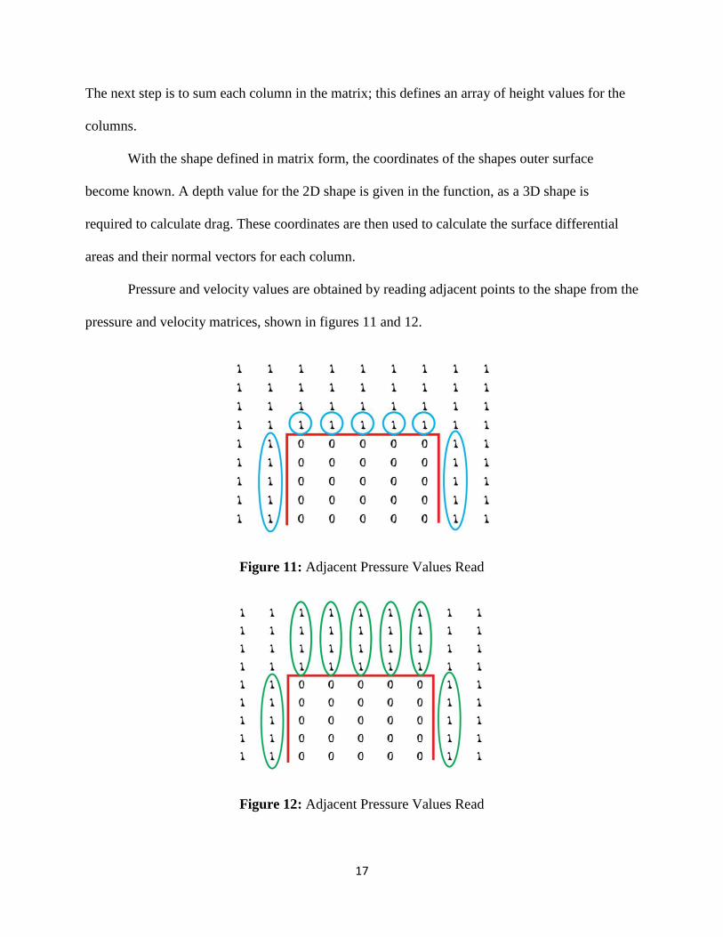
Pressure and velocity values are obtained by reading adjacent points to the shape from the

pressure and velocity matrices, shown in figures 11 and 12.

Figure 11: Adjacent Pressure Values Read

Figure 12: Adjacent Pressure Values Read

18

The pressure values are then multiplied by the computed surface areas and computed normal

vectors. The sum of these computed values is the total pressure drag. Several velocity values are

read for each column. The velocity values that are read are treated as differentials with respect to

y. These values are summed and multiplied by the computed surface areas and μ (the dynamic

viscosity of the fluid). This process makes an array of shear drag force values. Summing these

numbers gives the total shear drag on the shape. By adding up the pressure drag and shear drag

forces the total drag is found.

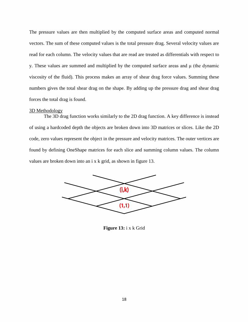
3D Methodology

The 3D drag function works similarly to the 2D drag function. A key difference is instead

of using a hardcoded depth the objects are broken down into 3D matrices or slices. Like the 2D

code, zero values represent the object in the pressure and velocity matrices. The outer vertices are

found by defining OneShape matrices for each slice and summing column values. The column

values are broken down into an i x k grid, as shown in figure 13.

Figure 13: i x k Grid

19

Each point on the square and its respective height values represent vertices on the object. The

vertices are entered into a function that calculates the area of a polygon in three-dimensional

space.

Figure 14: 3D Differential Area

Next the object’s adjacent points are read from the pressure and velocity matrices. In the same

manner as 2D, these values are used to calculate the pressure and shear forces acting on the

object. The sum of these values gives the total drag force.

Buchtel Community Learning Center Trial This April, the senior design team had the opportunity to participate in a trial of the Zipping

Towards STEM curriculum at Buchtel Community Learning Center (CLC). The trial, consisting

of five current 8th grade students, allowed the senior design team the chance to see how well the

simulation wind tunnel would work when used by the target audience. Over the course of the five

day trial, the 8th grade students were able to:

1. Learn the basics of aerodynamics using the 2D functionality of the simulation wind

tunnel

2. Design their own soap box derby mini car using 123D Design

20

3. Test the projected performance of their car design using the 3D functionality of the simulation

wind tunnel

4. Redesign their car in an attempt to make it more aerodynamic

5. 3D print their final design

6. Test their soap box derby mini car in an actual wind tunnel

7. Race against the other car designs on a mini track

The trial was extremely helpful to the team and resulted in many upgrades to the simulation wind

tunnel software.

Conclusion Through a concentrated effort and weekly team meetings, the team was able to meet the

trial deadline that had been set to test the curriculum this spring at Buchtel CLC. Since the program

is able to run its analysis in a matter of minutes, it provides the student with results in a time frame

which suits the Zipping Towards STEM curriculum. While the program may not predict a drag

output as accurate as commercial CFD programs can, it provides an output that enables the student

to predict which shapes and objects are more aerodynamic than others. This balance between time

and accuracy was developed taking into account the brief attention span of adolescent students

who are waiting for answers. The whole Zipping Towards STEM curriculum will be tested next

year (2016-2017) in a select few Akron Public School 8th grade classrooms. The following year

(2017-2018) the program will be expanded to all Akron Public School 8th graders in a hope to

provide the engineering education that many K-12 STEM programs are missing.

21

References

[1] Siebold, B. 2008, “A Compact and fast Matlab code solving the incompressible Navier-Stokes

equations on rectangular domains”

[2] 2015, "Navier -Stokes Equations", from https://www.grc.nasa.gov/www/k-

12/airplane/nseqs.html

[3] Munson, Bruce, Theodore Okiishi, Wade Huebsch, and Alric Rothmayer. Fluid Mechanics.

John Wiley and Sons Singapore Pte. Ltd. 2013.