Özgür L. Özçep

INSTITUT FÜR INFORMATIONSSYSTEME

Data Exchange 1Lecture 5: Motivation, Relational DE, Chase

16 November, 2016

Foundations of Ontologies and Databasesfor Information SystemsCS5130 (Winter 16/17)

Recap of Lecture 4

One of these Lectures ...

I Last lecture was better than the one of last year. Nonetheless,the following video is worth watching:

I https://www.youtube.com/watch?v=IQgAuBhlBT0Owl video

3 / 71

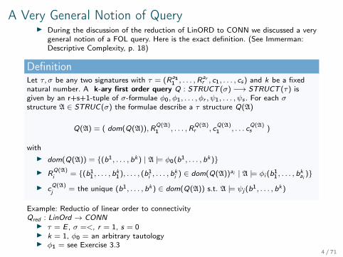
A Very General Notion of QueryI During the discussion of the reduction of LinORD to CONN we discussed a very

general notion of a FOL query. Here is the exact definition. (See Immerman:Descriptive Complexity, p. 18)

DefinitionLet τ, σ be any two signatures with τ = (Ra1

1 , . . . ,Rarr , c1, . . . , cs) and k be a fixed

natural number. A k-ary first order query Q : STRUCT (σ) −→ STRUCT (τ) isgiven by an r+s+1-tuple of σ-formulae φ0, φ1, . . . , φr , ψ1, . . . , ψs . For each σstructure A ∈ STRUC(σ) the formulae describe a τ structure Q(A)

Q(A) = ( dom(Q(A)),RQ(A)1 , . . . ,R

Q(A)r , c

Q(A)1 , . . . c

Q(A)s )

withI dom(Q(A)) = {(b1, . . . , bk ) | A |= φ0(b1, . . . , bk )}I R

Q(A)i = {(b1

1 , . . . , bk1), . . . , (b

1i , . . . , b

ki ) ∈ dom(Q(A))ai | A |= φi (b

11 , . . . , b

kai)}

I cQ(A)j = the unique (b1, . . . , bk ) ∈ dom(Q(A)) s.t. A |= ψj (b

1, . . . , bk )

Example: Reductio of linear order to connectivityQred : LinOrd → CONNI τ = E , σ =<, r = 1, s = 0I k = 1, φ0 = an arbitrary tautologyI φ1 = see Exercise 3.3

4 / 71

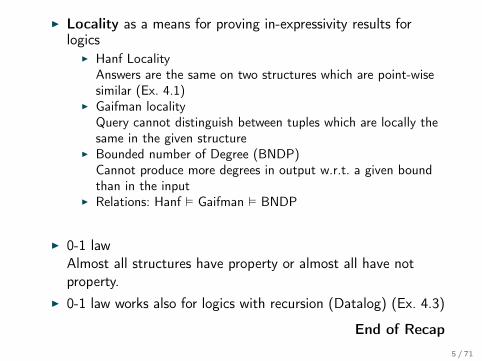
I Locality as a means for proving in-expressivity results forlogics

I Hanf LocalityAnswers are the same on two structures which are point-wisesimilar (Ex. 4.1)

I Gaifman localityQuery cannot distinguish between tuples which are locally thesame in the given structure

I Bounded number of Degree (BNDP)Cannot produce more degrees in output w.r.t. a given boundthan in the input

I Relations: Hanf � Gaifman � BNDP

I 0-1 lawAlmost all structures have property or almost all have notproperty.

I 0-1 law works also for logics with recursion (Datalog) (Ex. 4.3)

End of Recap5 / 71

Data Exchange: Motivation

References

I (Arenas et al., 2014)M. Arenas, P. Barceló, L. Libkin, and F. Murlak. Foundationsof Data Exchange. Cambridge University Press, 2014.

I M. Arenas: Slides to “Data Exchange in the Relational andRDF Worlds”, Fifth Workshop on Semantic Web InformationManagement 2011

7 / 71

Data Exchange History

I Much research in DB community

I Incorporated into IBM Clio

I Formal treatment starts with 2003 paper by Fagin andcolleaguesLit: R. Fagin, L. M. Haas, M. Hernández, R. J. Miller, L. Popa, and Y.

Velegrakis. Conceptual modeling: Foundations and applications. chapter Clio:

Schema Mapping Creation and Data Exchange, pages 198–236. Springer-Verlag,

Berlin, Heidelberg, 2009.

Lit: R. Fagin et al. Data exchange: Semantics and query answering. In:

Database Theory - ICDT 2003, 2003, Proceedings, volume 2572 of LNCS, pages

207–224. Springer, 2003.

8 / 71

Semantic Integration

I Data Exchange a form of semantic integration

I Research area semantic integration (SI)Deals with issues related to ensuring interoperability ofpossibly heterogeneous data sources.

I Lecture 5 and 6: Data Exchange: Directed DB-level SI forsource and target DB

I Following lecturesI OBDA: Bridging the DB and ontology worldI Ontology-level integration

9 / 71

Data Exchange (DE)I DE deals in a specific way with the integration of DBsI Heterogeneity: Two DBs on the same domain but different

schemata, σ (source) and τ (target)

I Interoperability: Relationship specifications Mτσ for σ and τ

I Relevant service: Query answering over τ

I ChallengesI Consistency: Is there a corresponding τ instance for a given σ

instance?I Materialization: If yes, construct and materialize exactly one

instance for τI Query answering: Answer query on this instance (using

rewriting)I Maintenance: How to construct/maintain mappings

10 / 71

Data Exchange (DE)I DE deals in a specific way with the integration of DBsI Heterogeneity: Two DBs on the same domain but different

schemata, σ (source) and τ (target)

I Interoperability: Relationship specifications Mτσ for σ and τ

I Relevant service: Query answering over τ

I ChallengesI Consistency: Is there a corresponding τ instance for a given σ

instance?I Materialization: If yes, construct and materialize exactly one

instance for τI Query answering: Answer query on this instance (using

rewriting)I Maintenance: How to construct/maintain mappings

11 / 71

Relational DE

I Going to deal mainly with relational DBs

I Language for specifying Mστ : Specific FOL formulas calledtuple generating dependencies (tgds)

I Allow for constraints on the target schema (such as foreignkeys)

I Explicate criteria for goodness of solutions by universalmodel and core notion

I Query answering w.r.t. certain answer semantics and usingrewriting

12 / 71

Running Example: Flight Domain

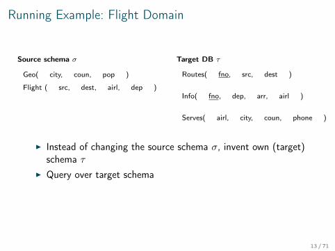
Source schema σ

Geo( city, coun, pop )

Flight ( src, dest, airl, dep )

Target DB τ

Routes( fno, src, dest )

Info( fno, dep, arr, airl )

Serves( airl, city, coun, phone )

I Instead of changing the source schema σ, invent own (target)schema τ

I Query over target schema

13 / 71

Running Example: Flight Domain

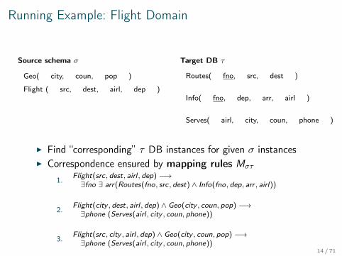
Source schema σ

Geo( city, coun, pop )

Flight ( src, dest, airl, dep )

Target DB τ

Routes( fno, src, dest )

Info( fno, dep, arr, airl )

Serves( airl, city, coun, phone )

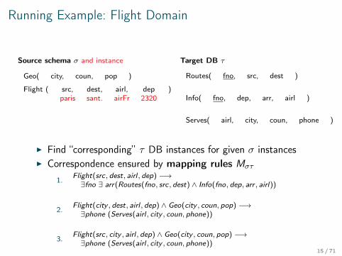
I Find “corresponding” τ DB instances for given σ instancesI Correspondence ensured by mapping rules Mστ

1. Flight(src, dest, airl , dep) −→∃fno ∃ arr(Routes(fno, src, dest) ∧ Info(fno, dep, arr , airl))

2. Flight(city , dest, airl , dep) ∧ Geo(city , coun, pop) −→∃phone (Serves(airl , city , coun, phone))

3. Flight(src, city , airl , dep) ∧ Geo(city , coun, pop) −→∃phone (Serves(airl , city , coun, phone))

14 / 71

Running Example: Flight Domain

Source schema σ and instance

Geo( city, coun, pop )

Flight ( src, dest, airl, dep )paris sant. airFr 2320

Target DB τ

Routes( fno, src, dest )

Info( fno, dep, arr, airl )

Serves( airl, city, coun, phone )

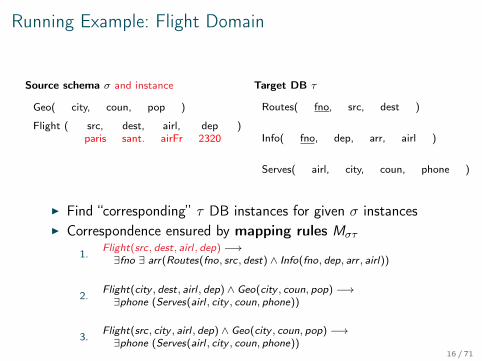
I Find “corresponding” τ DB instances for given σ instancesI Correspondence ensured by mapping rules Mστ

1. Flight(src, dest, airl , dep) −→∃fno ∃ arr(Routes(fno, src, dest) ∧ Info(fno, dep, arr , airl))

2. Flight(city , dest, airl , dep) ∧ Geo(city , coun, pop) −→∃phone (Serves(airl , city , coun, phone))

3. Flight(src, city , airl , dep) ∧ Geo(city , coun, pop) −→∃phone (Serves(airl , city , coun, phone))

15 / 71

Running Example: Flight Domain

Source schema σ and instance

Geo( city, coun, pop )

Flight ( src, dest, airl, dep )paris sant. airFr 2320

Target DB τ

Routes( fno, src, dest )

Info( fno, dep, arr, airl )

Serves( airl, city, coun, phone )

I Find “corresponding” τ DB instances for given σ instancesI Correspondence ensured by mapping rules Mστ

1. Flight(src, dest, airl , dep) −→∃fno ∃ arr(Routes(fno, src, dest) ∧ Info(fno, dep, arr , airl))

2. Flight(city , dest, airl , dep) ∧ Geo(city , coun, pop) −→∃phone (Serves(airl , city , coun, phone))

3. Flight(src, city , airl , dep) ∧ Geo(city , coun, pop) −→∃phone (Serves(airl , city , coun, phone))

16 / 71

Running Example: Flight Domain

Source schema σ and instance

Geo( city, coun, pop )

Flight ( src, dest, airl, dep )paris sant. airFr 2320

Target DB τ and instance

Routes( fno, src, dest )⊥1, paris, sant.

Info( fno, dep, arr, airl )⊥1, 2320, ⊥2 airFr

Serves( airl, city, coun, phone )

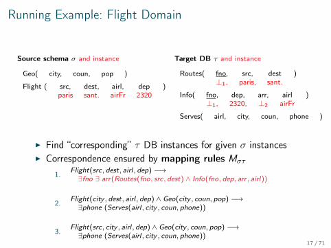
I Find “corresponding” τ DB instances for given σ instancesI Correspondence ensured by mapping rules Mστ

1. Flight(src, dest, airl , dep) −→∃fno ∃ arr(Routes(fno, src, dest) ∧ Info(fno, dep, arr , airl))

2. Flight(city , dest, airl , dep) ∧ Geo(city , coun, pop) −→∃phone (Serves(airl , city , coun, phone))

3. Flight(src, city , airl , dep) ∧ Geo(city , coun, pop) −→∃phone (Serves(airl , city , coun, phone))

17 / 71

Running Example: Flight Domain

Source schema σ and instance

Geo( city, coun, pop )

Flight ( src, dest, airl, dep )paris sant. airFr 2320

Target DB τ and instance

Routes( fno, src, dest )⊥1, paris, sant.

Info( fno, dep, arr, airl )⊥1, 2320, ⊥2 airFr

Serves( airl, city, coun, phone )

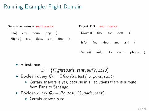
I σ-instanceS = {Flight(paris, sant, airFr , 2320)}

I τ solutionT = {Routes(⊥1, paris, sant), Info(⊥1, 2320,⊥2, airFr)}

I In general there may be more than one solution:T′ = {Routes(123, paris, sant), Info(123, 2320,⊥2, airFr)}

I Have to answer queries w.r.t. all solutions: certain answers18 / 71

Running Example: Flight Domain

Source schema σ and instance

Geo( city, coun, pop )

Flight ( src, dest, airl, dep )

Target DB τ and instance

Routes( fno, src, dest )

Info( fno, dep, arr, airl )

Serves( airl, city, coun, phone )

I σ-instanceS = {Flight(paris, sant, airFr , 2320)

I Boolean query Q1 = ∃fno Routes(fno, paris, sant)I Certain answers is yes, because in all solutions there is a route

form Paris to SantiagoI Boolean query Q2 = Routes(123, paris, sant)

I Certain answer is no

19 / 71

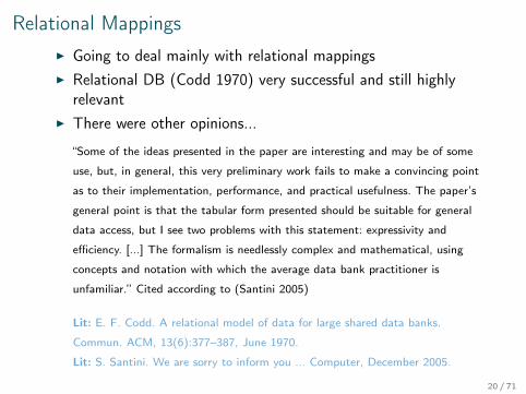
Relational MappingsI Going to deal mainly with relational mappingsI Relational DB (Codd 1970) very successful and still highly

relevantI There were other opinions...

“Some of the ideas presented in the paper are interesting and may be of some

use, but, in general, this very preliminary work fails to make a convincing point

as to their implementation, performance, and practical usefulness. The paper’s

general point is that the tabular form presented should be suitable for general

data access, but I see two problems with this statement: expressivity and

efficiency. [...] The formalism is needlessly complex and mathematical, using

concepts and notation with which the average data bank practitioner is

unfamiliar.” Cited according to (Santini 2005)

Lit: E. F. Codd. A relational model of data for large shared data banks.

Commun. ACM, 13(6):377–387, June 1970.

Lit: S. Santini. We are sorry to inform you ... Computer, December 2005.

20 / 71

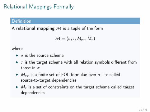
Relational Mappings Formally

DefinitionA relational mapping M is a tuple of the form

M = (σ, τ,Mστ ,Mτ )

whereI σ is the source schemaI τ is the target schema with all relation symbols different from

those in σI Mστ is a finite set of FOL formulae over σ ∪ τ called

source-to-target dependenciesI Mτ is a set of constraints on the target schema called target

dependencies

21 / 71

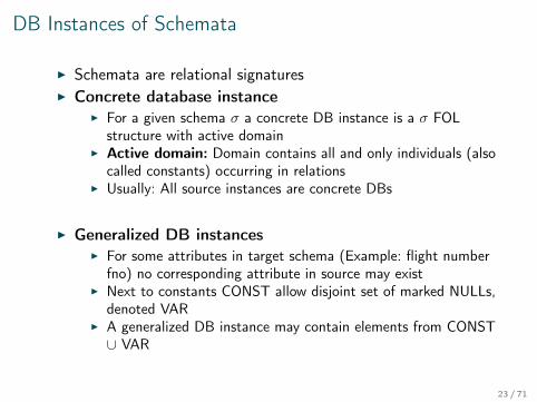
DB Instances of Schemata

I Schemata are relational signaturesI Concrete database instance

I For a given schema σ a concrete DB instance is a σ FOLstructure with active domain

I Active domain: Domain contains all and only individuals (alsocalled constants) occurring in relations

I Usually: All source instances are concrete DBs

I Generalized DB instancesI For some attributes in target schema (Example: flight number

fno) no corresponding attribute in source may existI Next to constants CONST allow disjoint set of marked NULLs,

denoted VARI A generalized DB instance may contain elements from CONST∪ VAR

22 / 71

DB Instances of Schemata

I Schemata are relational signaturesI Concrete database instance

I For a given schema σ a concrete DB instance is a σ FOLstructure with active domain

I Active domain: Domain contains all and only individuals (alsocalled constants) occurring in relations

I Usually: All source instances are concrete DBs

I Generalized DB instancesI For some attributes in target schema (Example: flight number

fno) no corresponding attribute in source may existI Next to constants CONST allow disjoint set of marked NULLs,

denoted VARI A generalized DB instance may contain elements from CONST∪ VAR

23 / 71

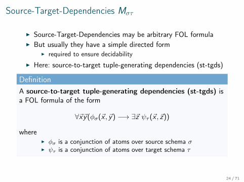
Source-Target-Dependencies Mστ

I Source-Target-Dependencies may be arbitrary FOL formulaI But usually they have a simple directed form

I required to ensure decidability

I Here: source-to-target tuple-generating dependencies (st-tgds)

DefinitionA source-to-target tuple-generating dependencies (st-tgds) isa FOL formula of the form

∀~x~y(φσ(~x , ~y) −→ ∃~z ψτ (~x , ~z))

whereI φσ is a conjunction of atoms over source schema σI ψτ is a conjunction of atoms over target schema τ

24 / 71

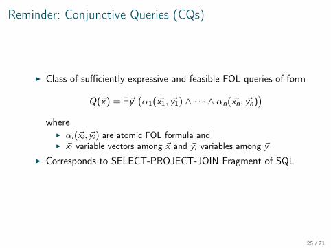
Reminder: Conjunctive Queries (CQs)

I Class of sufficiently expressive and feasible FOL queries of form

Q(~x) = ∃~y(α1(~x1, ~y1) ∧ · · · ∧ αn(~xn, ~yn)

)where

I αi (~xi , ~yi ) are atomic FOL formula andI ~xi variable vectors among ~x and ~yi variables among ~y

I Corresponds to SELECT-PROJECT-JOIN Fragment of SQL

25 / 71

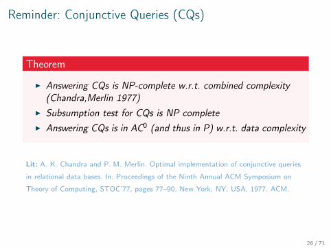
Reminder: Conjunctive Queries (CQs)

Theorem

I Answering CQs is NP-complete w.r.t. combined complexity(Chandra,Merlin 1977)

I Subsumption test for CQs is NP completeI Answering CQs is in AC0 (and thus in P) w.r.t. data complexity

Lit: A. K. Chandra and P. M. Merlin. Optimal implementation of conjunctive queries

in relational data bases. In: Proceedings of the Ninth Annual ACM Symposium on

Theory of Computing, STOC’77, pages 77–90, New York, NY, USA, 1977. ACM.

26 / 71

Wake-Up Question

Are st-tgds Datalog rules?

27 / 71

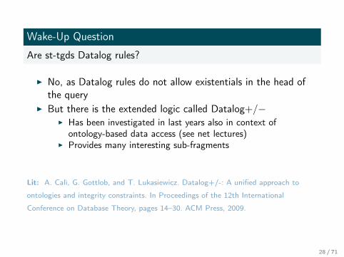
Wake-Up Question

Are st-tgds Datalog rules?

I No, as Datalog rules do not allow existentials in the head ofthe query

I But there is the extended logic called Datalog+/−I Has been investigated in last years also in context of

ontology-based data access (see net lectures)I Provides many interesting sub-fragments

Lit: A. Calì, G. Gottlob, and T. Lukasiewicz. Datalog+/-: A unified approach to

ontologies and integrity constraints. In Proceedings of the 12th International

Conference on Database Theory, pages 14–30. ACM Press, 2009.

28 / 71

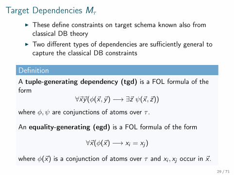
Target Dependencies Mτ

I These define constraints on target schema known also fromclassical DB theory

I Two different types of dependencies are sufficiently general tocapture the classical DB constraints

DefinitionA tuple-generating dependency (tgd) is a FOL formula of theform

∀~x~y(φ(~x , ~y) −→ ∃~z ψ(~x , ~z))

where φ, ψ are conjunctions of atoms over τ .

An equality-generating (egd) is a FOL formula of the form

∀~x(φ(~x) −→ xi = xj)

where φ(~x) is a conjunction of atoms over τ and xi , xj occur in ~x .

29 / 71

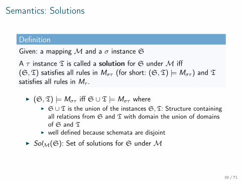
Semantics: Solutions

DefinitionGiven: a mappingM and a σ instance S

A τ instance T is called a solution for S underM iff(S,T) satisfies all rules in Mστ (for short: (S,T) |= Mστ ) and Tsatisfies all rules in Mτ .

I (S,T) |= Mστ iff S ∪ T |= Mστ whereI S ∪ T is the union of the instances S,T: Structure containing

all relations from S and T with domain the union of domainsof S and T

I well defined because schemata are disjoint

I SolM(S): Set of solutions for S underM

30 / 71

First Key Problem: Existence of Solutions

Problem: SOLEXISTENCEMInput: Source instance SOutput: Answer whether there exists a solution for S underM

I Note:M is assumed to be fixed =⇒ data complexityI This problem is going to be approached with a well known

proof tool: chase

31 / 71

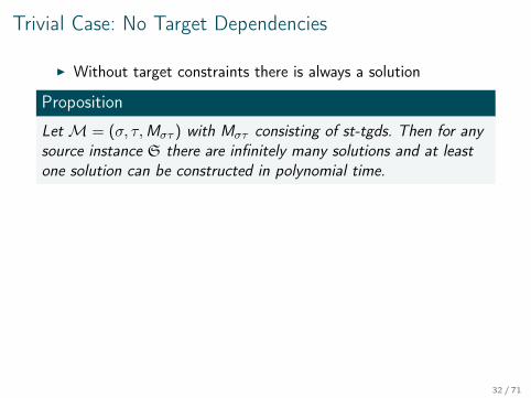
Trivial Case: No Target Dependencies

I Without target constraints there is always a solution

Proposition

LetM = (σ, τ,Mστ ) with Mστ consisting of st-tgds. Then for anysource instance S there are infinitely many solutions and at leastone solution can be constructed in polynomial time.

Proof IdeaI For every rule and every tuple ~a fulfilling the head generate

facts according to the body (using fresh named nulls for theexistentially quantified variables)

I Resulting τ instance T is a solutionI Polynomial: Testing whether ~a fulfills the head (a conjunctive

query) can be done in polynomial timeI Infinity: From T can build any other solution by extension

32 / 71

Trivial Case: No Target Dependencies

I Without target constraints there is always a solution

Proposition

LetM = (σ, τ,Mστ ) with Mστ consisting of st-tgds. Then for anysource instance S there are infinitely many solutions and at leastone solution can be constructed in polynomial time.

Proof IdeaI For every rule and every tuple ~a fulfilling the head generate

facts according to the body (using fresh named nulls for theexistentially quantified variables)

I Resulting τ instance T is a solutionI Polynomial: Testing whether ~a fulfills the head (a conjunctive

query) can be done in polynomial timeI Infinity: From T can build any other solution by extension

33 / 71

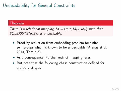
Undecidability for General Constraints

TheoremThere is a relational mappingM = (σ, τ,Mστ ,Mτ ) such thatSOLEXISTENCEM is undecidable.

I Proof by reduction from embedding problem for finitesemigroups which is known to be undecidable (Arenas et al.2014, Thm 5.3)

I As a consequence: Further restrict mapping rulesI But note that the following chase construction defined for

arbitrary st-tgds

34 / 71

Undecidability for General Constraints

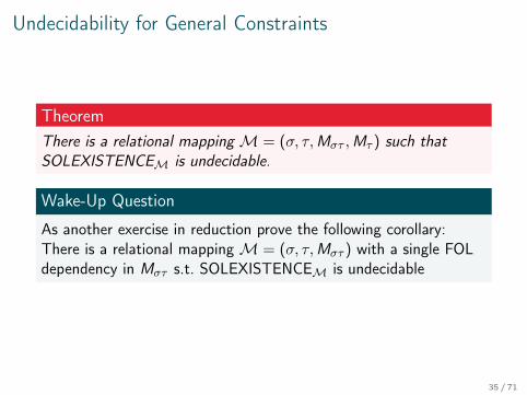
TheoremThere is a relational mappingM = (σ, τ,Mστ ,Mτ ) such thatSOLEXISTENCEM is undecidable.

Wake-Up Question

As another exercise in reduction prove the following corollary:There is a relational mappingM = (σ, τ,Mστ ) with a single FOLdependency in Mστ s.t. SOLEXISTENCEM is undecidable

35 / 71

Undecidability for General Constraints

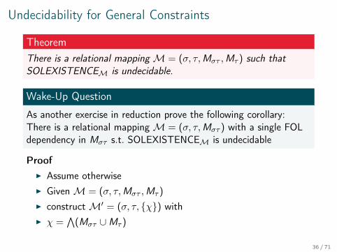
TheoremThere is a relational mappingM = (σ, τ,Mστ ,Mτ ) such thatSOLEXISTENCEM is undecidable.

Wake-Up Question

As another exercise in reduction prove the following corollary:There is a relational mappingM = (σ, τ,Mστ ) with a single FOLdependency in Mστ s.t. SOLEXISTENCEM is undecidable

ProofI Assume otherwiseI GivenM = (σ, τ,Mστ ,Mτ )

I constructM′ = (σ, τ, {χ}) withI χ =

∧(Mστ ∪Mτ )

36 / 71

Existence Proof vs. Construction

I Proposition above showed existence of solutionI Showing existence 6= construction a verifierI Actually we are going to construct a solution using the chase

I Interesting debate in philosophy of mathematics whethernon-constructive proofs are acceptable

I Mathematical Intuitionism: field allowing only constructiveproofs

I truth = provable = constructively provableI Classical logical inference rules s.a. ¬¬A � A not allowedI Main inventor: L.E.J. Brouwer (1881 to 1966)

Irony: Has many interesting results in classical(non-constructive) mathematics (Brouwer’s fixed pointtheorem)

37 / 71

Chase Construction

I A widely used tool in DB theoryI Original use: Calculating entailments of DB constraints

Lit: D. Maier, A. O. Mendelzon, and Y. Sagiv. Testing implications of data

dependencies. ACM Trans. Database Syst., 4(4):455–469, Dec. 1979.

I General ideaI Apply tgds as completion/repair rules in a bottom-up strategyI until no tgds can be applied anymoreI Chase construction mail fail if one of the egds is violated

I The chase leads to an instance with desirable propertiesI It produces not too many redundant factsI Universality

38 / 71

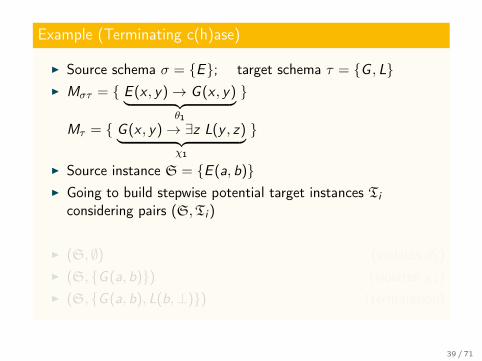
Example (Terminating c(h)ase)

I Source schema σ = {E}; target schema τ = {G , L}I Mστ = { E (x , y)→ G (x , y)︸ ︷︷ ︸

θ1

}

Mτ = { G (x , y)→ ∃z L(y , z)︸ ︷︷ ︸χ1

}

I Source instance S = {E (a, b)}I Going to build stepwise potential target instances Ti

considering pairs (S,Ti )

I (S, ∅) (violates θ1)I (S, {G (a, b)}) (violates χ1)I (S, {G (a, b), L(b,⊥)}) (termination)

39 / 71

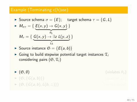
Example (Terminating c(h)ase)

I Source schema σ = {E}; target schema τ = {G , L}I Mστ = { E (x , y)→ G (x , y)︸ ︷︷ ︸

θ1

}

Mτ = { G (x , y)→ ∃z L(y , z)︸ ︷︷ ︸χ1

}

I Source instance S = {E (a, b)}I Going to build stepwise potential target instances Ti

considering pairs (S,Ti )

I (S, ∅) (violates θ1)I (S, {G (a, b)}) (violates χ1)I (S, {G (a, b), L(b,⊥)}) (termination)

40 / 71

Example (Terminating c(h)ase)

I Source schema σ = {E}; target schema τ = {G , L}I Mστ = { E (x , y)→ G (x , y)︸ ︷︷ ︸

θ1

}

Mτ = { G (x , y)→ ∃z L(y , z)︸ ︷︷ ︸χ1

}

I Source instance S = {E (a, b)}I Going to build stepwise potential target instances Ti

considering pairs (S,Ti )

I (S, ∅) (violates θ1)I (S, {G (a, b)}) (violates χ1)I (S, {G (a, b), L(b,⊥)}) (termination)

41 / 71

Example (Terminating c(h)ase)

I Source schema σ = {E}; target schema τ = {G , L}I Mστ = { E (x , y)→ G (x , y)︸ ︷︷ ︸

θ1

}

Mτ = { G (x , y)→ ∃z L(y , z)︸ ︷︷ ︸χ1

}

I Source instance S = {E (a, b)}I Going to build stepwise potential target instances Ti

considering pairs (S,Ti )

I (S, ∅) (violates θ1)I (S, {G (a, b)}) (violates χ1)I (S, {G (a, b), L(b,⊥)}) (termination)

42 / 71

Example (Terminating c(h)ase)

I Source schema σ = {E}; target schema τ = {G , L}I Mστ = { E (x , y)→ G (x , y)︸ ︷︷ ︸

θ1

}

Mτ = { G (x , y)→ ∃z L(y , z)︸ ︷︷ ︸χ1

}

I Source instance S = {E (a, b)}I Going to build stepwise potential target instances Ti

considering pairs (S,Ti )

I (S, ∅) (violates θ1)I (S, {G (a, b)}) (violates χ1)I (S, {G (a, b), L(b,⊥)}) (termination)

43 / 71

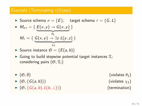
Example (Terminating c(h)ase)

I Source schema σ = {E}; target schema τ = {G , L}I Mστ = { E (x , y)→ G (x , y)︸ ︷︷ ︸

θ1

}

Mτ = { G (x , y)→ ∃z L(y , z)︸ ︷︷ ︸χ1

}

I Source instance S = {E (a, b)}I Going to build stepwise potential target instances Ti

considering pairs (S,Ti )

I (S, ∅) (violates θ1)I (S, {G (a, b)}) (violates χ1)I (S, {G (a, b), L(b,⊥)}) (termination)

44 / 71

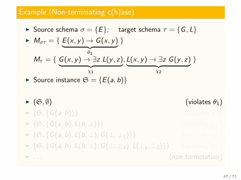
Example (Non-terminating c(h)ase)

I Source schema σ = {E}; target schema τ = {G , L}I Mστ = { E (x , y)→ G (x , y)︸ ︷︷ ︸

θ1

}

Mτ = { G (x , y)→ ∃z L(y , z)︸ ︷︷ ︸χ1

, L(x , y)→ ∃z G (y , z)︸ ︷︷ ︸χ2

}

I Source instance S = {E (a, b)}

I (S, ∅) (violates θ1)I (S, {G (a, b)}) (violates χ1)I (S, {G (a, b), L(b,⊥)}) (violates χ2 )I (S, {G (a, b), L(b,⊥),G (⊥,⊥1)}) (violates χ1 )I (S, {G (a, b), L(b,⊥),G (⊥,⊥1), L(⊥1,⊥2)}) (violates χ2 )I . . . (non-termination)

45 / 71

Example (Non-terminating c(h)ase)

I Source schema σ = {E}; target schema τ = {G , L}I Mστ = { E (x , y)→ G (x , y)︸ ︷︷ ︸

θ1

}

Mτ = { G (x , y)→ ∃z L(y , z)︸ ︷︷ ︸χ1

, L(x , y)→ ∃z G (y , z)︸ ︷︷ ︸χ2

}

I Source instance S = {E (a, b)}

I (S, ∅) (violates θ1)I (S, {G (a, b)}) (violates χ1)I (S, {G (a, b), L(b,⊥)}) (violates χ2 )I (S, {G (a, b), L(b,⊥),G (⊥,⊥1)}) (violates χ1 )I (S, {G (a, b), L(b,⊥),G (⊥,⊥1), L(⊥1,⊥2)}) (violates χ2 )I . . . (non-termination)

46 / 71

Example (Non-terminating c(h)ase)

I Source schema σ = {E}; target schema τ = {G , L}I Mστ = { E (x , y)→ G (x , y)︸ ︷︷ ︸

θ1

}

Mτ = { G (x , y)→ ∃z L(y , z)︸ ︷︷ ︸χ1

, L(x , y)→ ∃z G (y , z)︸ ︷︷ ︸χ2

}

I Source instance S = {E (a, b)}

I (S, ∅) (violates θ1)I (S, {G (a, b)}) (violates χ1)I (S, {G (a, b), L(b,⊥)}) (violates χ2 )I (S, {G (a, b), L(b,⊥),G (⊥,⊥1)}) (violates χ1 )I (S, {G (a, b), L(b,⊥),G (⊥,⊥1), L(⊥1,⊥2)}) (violates χ2 )I . . . (non-termination)

47 / 71

Example (Non-terminating c(h)ase)

I Source schema σ = {E}; target schema τ = {G , L}I Mστ = { E (x , y)→ G (x , y)︸ ︷︷ ︸

θ1

}

Mτ = { G (x , y)→ ∃z L(y , z)︸ ︷︷ ︸χ1

, L(x , y)→ ∃z G (y , z)︸ ︷︷ ︸χ2

}

I Source instance S = {E (a, b)}

I (S, ∅) (violates θ1)I (S, {G (a, b)}) (violates χ1)I (S, {G (a, b), L(b,⊥)}) (violates χ2 )I (S, {G (a, b), L(b,⊥),G (⊥,⊥1)}) (violates χ1 )I (S, {G (a, b), L(b,⊥),G (⊥,⊥1), L(⊥1,⊥2)}) (violates χ2 )I . . . (non-termination)

48 / 71

Example (Non-terminating c(h)ase)

I Source schema σ = {E}; target schema τ = {G , L}I Mστ = { E (x , y)→ G (x , y)︸ ︷︷ ︸

θ1

}

Mτ = { G (x , y)→ ∃z L(y , z)︸ ︷︷ ︸χ1

, L(x , y)→ ∃z G (y , z)︸ ︷︷ ︸χ2

}

I Source instance S = {E (a, b)}

I (S, ∅) (violates θ1)I (S, {G (a, b)}) (violates χ1)I (S, {G (a, b), L(b,⊥)}) (violates χ2 )I (S, {G (a, b), L(b,⊥),G (⊥,⊥1)}) (violates χ1 )I (S, {G (a, b), L(b,⊥),G (⊥,⊥1), L(⊥1,⊥2)}) (violates χ2 )I . . . (non-termination)

49 / 71

Example (Non-terminating c(h)ase)

I Source schema σ = {E}; target schema τ = {G , L}I Mστ = { E (x , y)→ G (x , y)︸ ︷︷ ︸

θ1

}

Mτ = { G (x , y)→ ∃z L(y , z)︸ ︷︷ ︸χ1

, L(x , y)→ ∃z G (y , z)︸ ︷︷ ︸χ2

}

I Source instance S = {E (a, b)}

I (S, ∅) (violates θ1)I (S, {G (a, b)}) (violates χ1)I (S, {G (a, b), L(b,⊥)}) (violates χ2 )I (S, {G (a, b), L(b,⊥),G (⊥,⊥1)}) (violates χ1 )I (S, {G (a, b), L(b,⊥),G (⊥,⊥1), L(⊥1,⊥2)}) (violates χ2 )I . . . (non-termination)

50 / 71

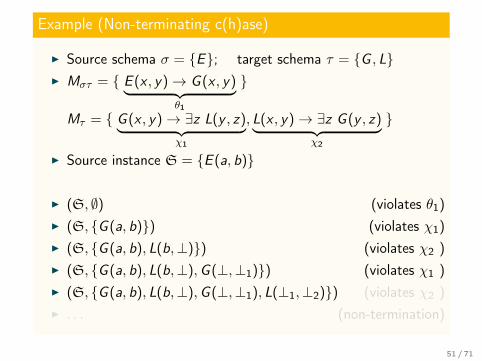
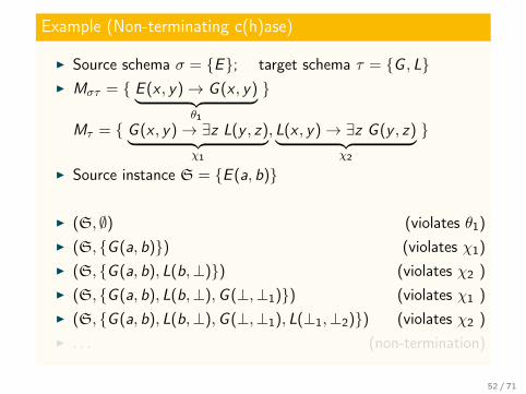
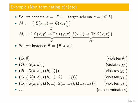
Example (Non-terminating c(h)ase)

I Source schema σ = {E}; target schema τ = {G , L}I Mστ = { E (x , y)→ G (x , y)︸ ︷︷ ︸

θ1

}

Mτ = { G (x , y)→ ∃z L(y , z)︸ ︷︷ ︸χ1

, L(x , y)→ ∃z G (y , z)︸ ︷︷ ︸χ2

}

I Source instance S = {E (a, b)}

I (S, ∅) (violates θ1)I (S, {G (a, b)}) (violates χ1)I (S, {G (a, b), L(b,⊥)}) (violates χ2 )I (S, {G (a, b), L(b,⊥),G (⊥,⊥1)}) (violates χ1 )I (S, {G (a, b), L(b,⊥),G (⊥,⊥1), L(⊥1,⊥2)}) (violates χ2 )I . . . (non-termination)

51 / 71

Example (Non-terminating c(h)ase)

I Source schema σ = {E}; target schema τ = {G , L}I Mστ = { E (x , y)→ G (x , y)︸ ︷︷ ︸

θ1

}

Mτ = { G (x , y)→ ∃z L(y , z)︸ ︷︷ ︸χ1

, L(x , y)→ ∃z G (y , z)︸ ︷︷ ︸χ2

}

I Source instance S = {E (a, b)}

I (S, ∅) (violates θ1)I (S, {G (a, b)}) (violates χ1)I (S, {G (a, b), L(b,⊥)}) (violates χ2 )I (S, {G (a, b), L(b,⊥),G (⊥,⊥1)}) (violates χ1 )I (S, {G (a, b), L(b,⊥),G (⊥,⊥1), L(⊥1,⊥2)}) (violates χ2 )I . . . (non-termination)

52 / 71

Example (Non-terminating c(h)ase)

I Source schema σ = {E}; target schema τ = {G , L}I Mστ = { E (x , y)→ G (x , y)︸ ︷︷ ︸

θ1

}

Mτ = { G (x , y)→ ∃z L(y , z)︸ ︷︷ ︸χ1

, L(x , y)→ ∃z G (y , z)︸ ︷︷ ︸χ2

}

I Source instance S = {E (a, b)}

I (S, ∅) (violates θ1)I (S, {G (a, b)}) (violates χ1)I (S, {G (a, b), L(b,⊥)}) (violates χ2 )I (S, {G (a, b), L(b,⊥),G (⊥,⊥1)}) (violates χ1 )I (S, {G (a, b), L(b,⊥),G (⊥,⊥1), L(⊥1,⊥2)}) (violates χ2 )I . . . (non-termination)

53 / 71

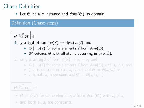
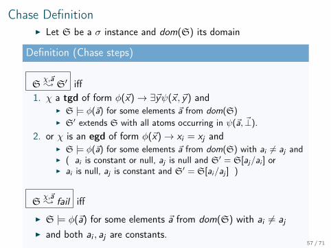
Chase DefinitionI Let S be a σ instance and dom(S) its domain

Definition (Chase steps)

Sχ,~a; S′ iff

1. χ a tgd of form φ(~x)→ ∃~yψ(~x , ~y) andI S |= φ(~a) for some elements ~a from dom(S)I S′ extends S with all atoms occurring in ψ(~a, ~⊥).

2. or χ is an egd of form φ(~x)→ xi = xj andI S |= φ(~a) for some elements ~a from dom(S) with ai 6= aj andI ( ai is constant or null, aj is null and S′ = S[aj/ai ] orI ai is null, aj is constant and S′ = S[ai/aj ] )

Sχ,~a; fail iff

I S |= φ(~a) for some elements ~a from dom(S) with ai 6= ajI and both ai , aj are constants.

54 / 71

Chase DefinitionI Let S be a σ instance and dom(S) its domain

Definition (Chase steps)

Sχ,~a; S′ iff

1. χ a tgd of form φ(~x)→ ∃~yψ(~x , ~y) andI S |= φ(~a) for some elements ~a from dom(S)I S′ extends S with all atoms occurring in ψ(~a, ~⊥).

2. or χ is an egd of form φ(~x)→ xi = xj andI S |= φ(~a) for some elements ~a from dom(S) with ai 6= aj andI ( ai is constant or null, aj is null and S′ = S[aj/ai ] orI ai is null, aj is constant and S′ = S[ai/aj ] )

Sχ,~a; fail iff

I S |= φ(~a) for some elements ~a from dom(S) with ai 6= ajI and both ai , aj are constants.

55 / 71

Chase DefinitionI Let S be a σ instance and dom(S) its domain

Definition (Chase steps)

Sχ,~a; S′ iff

1. χ a tgd of form φ(~x)→ ∃~yψ(~x , ~y) andI S |= φ(~a) for some elements ~a from dom(S)I S′ extends S with all atoms occurring in ψ(~a, ~⊥).

2. or χ is an egd of form φ(~x)→ xi = xj andI S |= φ(~a) for some elements ~a from dom(S) with ai 6= aj andI ( ai is constant or null, aj is null and S′ = S[aj/ai ] orI ai is null, aj is constant and S′ = S[ai/aj ] )

Sχ,~a; fail iff

I S |= φ(~a) for some elements ~a from dom(S) with ai 6= ajI and both ai , aj are constants.

56 / 71

Chase DefinitionI Let S be a σ instance and dom(S) its domain

Definition (Chase steps)

Sχ,~a; S′ iff

1. χ a tgd of form φ(~x)→ ∃~yψ(~x , ~y) andI S |= φ(~a) for some elements ~a from dom(S)I S′ extends S with all atoms occurring in ψ(~a, ~⊥).

2. or χ is an egd of form φ(~x)→ xi = xj andI S |= φ(~a) for some elements ~a from dom(S) with ai 6= aj andI ( ai is constant or null, aj is null and S′ = S[aj/ai ] orI ai is null, aj is constant and S′ = S[ai/aj ] )

Sχ,~a; fail iff

I S |= φ(~a) for some elements ~a from dom(S) with ai 6= ajI and both ai , aj are constants.

57 / 71

Chase

DefinitionA chase sequence for S under M is a sequence of chase steps

Siχi ,~ai; Si+1 such thatI S0 = S

I each χi is in M

I for each distinct i , j also (χi , ~ai ) 6= (χj , ~aj)

For a finite chase sequence the last instance is called its result.I If the result is fail , then the sequence is said to be a failing

sequenceI If no further dependency from M can be applied to a result,

then the sequence is called successful.

58 / 71

Indeterminism

I Indeterminism regarding choice of nulls (no problem)I Indeterminism regarding order of chosen tgds and egds

This may lead to different chase results

59 / 71

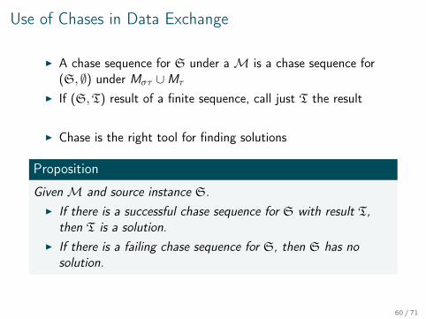
Use of Chases in Data Exchange

I A chase sequence for S under aM is a chase sequence for(S, ∅) under Mστ ∪Mτ

I If (S,T) result of a finite sequence, call just T the result

I Chase is the right tool for finding solutions

Proposition

GivenM and source instance S.I If there is a successful chase sequence for S with result T,

then T is a solution.I If there is a failing chase sequence for S, then S has no

solution.

60 / 71

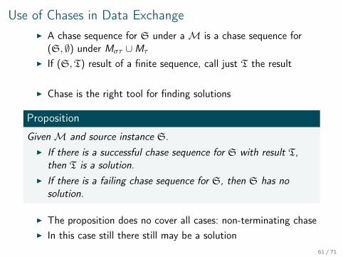
Use of Chases in Data ExchangeI A chase sequence for S under aM is a chase sequence for

(S, ∅) under Mστ ∪Mτ

I If (S,T) result of a finite sequence, call just T the result

I Chase is the right tool for finding solutions

Proposition

GivenM and source instance S.I If there is a successful chase sequence for S with result T,

then T is a solution.I If there is a failing chase sequence for S, then S has no

solution.

I The proposition does no cover all cases: non-terminating chaseI In this case still there still may be a solution

61 / 71

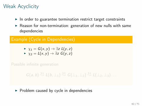
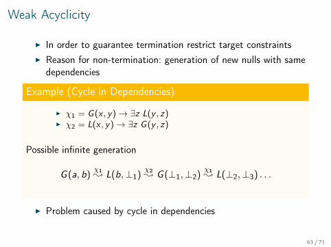
Weak Acyclicity

I In order to guarantee termination restrict target constraintsI Reason for non-termination: generation of new nulls with same

dependencies

Example (Cycle in Dependencies)

I χ1 = G (x , y)→ ∃z L(y , z)I χ2 = L(x , y)→ ∃z G (y , z)

Possible infinite generation

G (a, b)χ1; L(b,⊥1)

χ2; G (⊥1,⊥2)χ1; L(⊥2,⊥3) . . .

I Problem caused by cycle in dependencies

62 / 71

Weak Acyclicity

I In order to guarantee termination restrict target constraintsI Reason for non-termination: generation of new nulls with same

dependencies

Example (Cycle in Dependencies)

I χ1 = G (x , y)→ ∃z L(y , z)I χ2 = L(x , y)→ ∃z G (y , z)

Possible infinite generation

G (a, b)χ1; L(b,⊥1)

χ2; G (⊥1,⊥2)χ1; L(⊥2,⊥3) . . .

I Problem caused by cycle in dependencies

63 / 71

Simple Dependency GraphsI Nodes: pairs (R, i) of predicate R and argument-position iI Edges: From (Rb, i) to (Rh, j) iff there is a tgd∀~x∀~yφ(~x , ~y)→ ∃~zψ(~x , ~z) and1. Rh occurs in ψ and Rb occurs in φ and2. for all x ∈ ~x in i-position in Rb

I either x occurs in j-position in Rh

I or the variable in j-position in Rh is existentially quantified

Example (Simple Dependency Graph)

I χ1 = G (y , x)→ ∃z L(x , z)

I χ2 = L(y , x)→ ∃z G (x , z)

(L,1)

(G,1)

(L,2)

(G,2)

Set of tgds called acyclic if simple dependency graph is acyclic.64 / 71

Dependency Graphs (DG)I Nodes: pairs (R, i) of predicate R and argument-position iI Edges: From (Rb, i) to (Rh, j) iff there is a tgd∀~x∀~yφ(~x , ~y)→ ∃~zψ(~x , ~z) and1. Rh occurs in ψ and Rb occurs in φ and2. for all x ∈ ~x in i-position in Rb

I either x occurs in j-position in Rh

I or the variable in j-position in Rh is existentially quantifiedand and these are labelled by *

Example (Dependency Graph)

I χ1 = G (y , x)→ ∃z L(x , z)

I χ2 = L(y , x)→ ∃z G (x , z)

(L,1)

(G,1)

(L,2)

(G,2)

* *

TGDs weakly acyclic iff DG has no cycle with a * edge.65 / 71

Termination for weakly acyclic tgds

TheoremLetM = (σ, τ,Mστ ,Mτ ) be a mapping where Mτ is the union ofegds and weakly acyclic tgds. Then the length of every chasesequence for a source S is polynomially bounded w.r.t. the size ofS.

I In particular: Every chase sequence terminatesI Moreover: SOLEXISTENCEM can be solved in polynomial

timeI a solution can be constructed in polynomial time

66 / 71

Solutions to Exercise 4 (16 Points)

67 / 71

Solution to Exercise 4.1 (6 Points)Use Hanf locality in order to proof that the following booleanqueries are not FOL-definable: 1. graph acyclicity, 2. tree.

SolutionGraph Acyclicity (GA).I For contradiction assume GA is Hanf-local with parameter r ′. Choose

r = 2r ′ + 2I Let G be the disjoint union of a circle of length r and a linear order of length rI Let G′ be an order of length 2r .I Take a bijection f : G→ G′ where

I the circle is unravelled to the middle of G′.I The lower half part of the order in G is mapped to the lower

part of G′

I The upper half part of the order in G is mapped to the upperpart of G′

I an r ′-neighbourhood of any a in G and f (a) ∈ G′ is the same: if a is from thecircle in G then the r ′-neighbourhood is a 2r’-line and the same for f (a). If a isan element from the line in G then in its r ′-neighbourhood it has to the left andto right the same number of elements as has f (a) in its r’-neigbourhood in G′.

I Hence G�r′ G′, but: G is cyclic and G is not. E

TreeI Same construction (as G′ is tree whereas G is not)

68 / 71

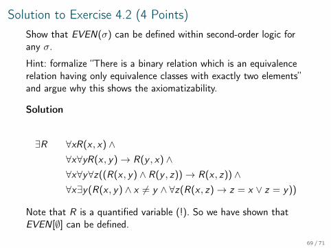
Solution to Exercise 4.2 (4 Points)Show that EVEN(σ) can be defined within second-order logic forany σ.

Hint: formalize “There is a binary relation which is an equivalencerelation having only equivalence classes with exactly two elements”and argue why this shows the axiomatizability.

Solution

∃R ∀xR(x , x) ∧∀x∀yR(x , y)→ R(y , x) ∧∀x∀y∀z((R(x , y) ∧ R(y , z))→ R(x , z)) ∧∀x∃y(R(x , y) ∧ x 6= y ∧ ∀z(R(x , z)→ z = x ∨ z = y))

Note that R is a quantified variable (!). So we have shown thatEVEN[∅] can be defined.

69 / 71

Solution to Exercise 4.3 (2 Points)

Argue why (in particular within the DB community) one imposessafety conditions for Datalog rules.

Solution

I Unsafe negation would lead to infinite answer sets (if domainis infinite.)

I Variables occurring only in head would lead to domaindependance. For example, for ans(x)← R(a) all bindings for xin the domain of a DB where R(a) is contained, would have tobe in the set of answers. So the answer would not depend onlyon R(a), i.e., only on the query, but also on the domain of thevariables one allows.

70 / 71

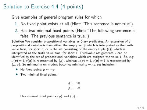
Solution to Exercise 4.4 (4 points)

Give examples of general program rules for which1. No fixed point exists at all (Hint: “This sentence is not true”)2. Has two minimal fixed points (Hint: “The following sentence is

false. The previous sentence is true.”)Solution We consider propositional variables as 0-ary predicates. An extension of apropositional variable is then either the empty set ∅ which is interpreted as the truthvalue false, for short 0, or is the set consisting of the empty tuple {()} which isinterpreted as the truth value true, for short 1. Truthvalue assignments ν can beidentified by the set of propositional variables which are assigned the value 1. So, e.g.,ν(p) = 1, ν(q) is represented by {p}, whereas ν(p) = 1, ν(q) = 1 is represented by{p, q}. So minimality on models becomes minimality w.r.t. set inclusion.I No fixed point: p ← ¬pI Two minimal fixed points.

q ← ¬pp ← ¬q

Has minimal fixed points {p} and {q}.

71 / 71