zen blue for axio imager blue - university of...
TRANSCRIPT

Ge#ng Started1. Switch on the white Power supply box.
Ø If you are using fluorescence switch on the HXP120 and Colibri control box.Ø If you are using ApoTome switch on the ApoTome box.
2. Switch on the microscope (at back leB of microscope stand).3. Switch on the computer and log on with your UQ username and password.4. Once the microscope has finished starJng up double click the Zen icon.
Ø When the menu appears, choose Zen Pro
Shu#ng Down1. Lower the stage and remove your sample.2. Gently wipe any oil objecJves you have used with lens 7ssue (do not use kim wipes to clean objec7ves).3. Exit the soBware and copy your files to your home or group network/USB drive.4. Turn off the microscope power supply box and the HXP120/Colibri/Apotome modules.
Visualising a Sample Through the Oculars1. On the touch screen aZached to the microscope press “load posi7on” and posiJon the slide on stage.
Pressing the buZon will return you to the working posiJon.
2. Press microscope (1) on the far leB of the touch screen.3. You will be able to change objec+ves, reflectors (filtersets) and adjust the light path via the tabs at the
top. (2)4. You can use one of the quick buZons at the boZom of the screen to get the microscope ready. (3)
Ø Press FL for fluorescence, BF for brigh`ield, PH for phase and DIC for DIC/Normaski Imaging modes.
Ø If imaging fluorescence ensure you have the appropriate fluorescent light switched on5. Check the light path is allowing the sample to be seen via the oculars (under the “light path” tab).
Ø Axio Imager: 100% tube (100% side port is for the colour camera only) and ensure the push-‐pull rod is all the way in.
Ø Axio Observer: 50 or 100% eyepiece/vis
6. An image will now be visible down the oculars -‐ adjust stage posiJon and focus as necessary.
1
Queensland Brain InsJtute Microscopy
Zeiss Axio Imager/Observer Guide
Queensland Brain InsJtute Microscopy

Imaging a Sample -‐ Using the Live Window1. Select an imaging mode on the touch screen.
Ø FL at the boZom leB for fluorescence.Ø BF/PH/DIC/DF for transmiZed light imaging.
2. Adjust the light path so light reaches the camera.Ø Axio Imager: Pull the push-‐pull rod on the side of the microscope out to the camera posiJon. Ø Axio Observer: In the light path menu on the touch screen – adjust the se#ngs to 100% camera.
3. Ensure the shuZers are open and illuminaJng the specimen.Ø Fluorescence -‐ both the reflected light shuZer (RL-‐shuOer via the touch screen) and the HXP lamp
shuZer (via the Colibri control panel – press the Ext. buOon (external light source) then press the shuOer buOon).
Ø BrighQield – the transmiZed light shuZer (TL-‐shuOer) (via the touch screen).4. Change to the acquisiJon tab (1) and choose a hardware configuraJon from the Experiment Manager (2)
(start with a configuraJon prefixed with “QBI” if a personalised se#ng does not exist).5. Open the Apotome Mode tool and uncheck Enable Apotome (3) if not using the Apotome module (if this
opJon remains checked the soBware will aZempt to calculate an opJcal secJon).6. Open the Channels tool and highlight the channel to be visualised (4) (the generic “QBI” configuraJon has
definiJons for the four main classes of fluorophores), make sure the correct camera is selected (5) and click the Exposure buZon (6).
7. Adjust exposure Jme by (7) pressing Set Exposure or using the Auto Exposure opJon. The Set Exposure buZon applies the hardware se#ngs and as such closes off the RL and External shuZers aBer the exposure Jme has been calculated. Using the Auto Exposure checkbox will dynamically calculate the exposure Jme such that this is adjusted each Jme the stage posiJon etc. changes.
8. Click Snap to create an image. Note: the images are captured but not saved at this point and are with an * to indicate as much.
2Queensland Brain InsJtute Microscopy
1
2
3
1
2
3

MulJdimensional AcquisiJonMulJdimensional acquisiJons can be achieved by choosing an Experiment(s) from the Experiment Manager (1). Checking the box next to the desired experiment adds a tool to the MulJdimensional AcquisiJon tab. Combining these experiments with channels selected in the Channels tool it is possible to create automated experimental protocols for single and mulJple channel imaging, Z-‐series, Jme-‐lapse and mosaic imaging or any combinaJon of these.The mul7dimensional acquisi7on op7ons:
Ø Z (Z-‐series): Image mulJple planes through Jssue/cells (page 6).Ø Tiles: Controls Jled image se#ngs for imaging across numerous
fields of view. This tool also includes an opJon for automated imaging a selected locaJons on your slide/dish in a similar way to Mark and Find in Axiovision (available on Green and Indigo).
Ø Time Series: Controls Jme-‐lapse se#ngs for live imaging of living cells/Jssues.
3
6
4
57
8
Queensland Brain InsJtute Microscopy
1

Hardware se#ngs for Axio Imagers / ObserversEach microscope has the opJon of using Colibri LEDs or the external HXP Xenon lamp for fluorescence. Colibri, when used with filterset 62, gives comparable and in some cases beZer results than using the HXP lamp, doesn’t change intensity as the LEDs age (unlike the HXP) and turns on instantly (no warm up or cool down Jme). You will need to use the HXP if you are using Alexa 546/555/568 or Cy3A recommended setup if you want to observe mul7ple proteins is:
DAPI + Alexa488/GFP + Alexa555 + Alexa647(Look out for crosstalk between Green and Red channels)
Another 4 colour combina7on is:
DAPI + Alexa488/GFP + Alexa594 + Alexa647 (Look out for crosstalk between Red and Far Red channels)
Experiment Seangs:
There are four generic predefined experiment configuraJons which you can adapt to your parJcular needs:1. QBI HXP (one for 5x to 20x ApoTome and one for 40x, 63x and 100x ApoTome)2. QBI Colibri (one for 5x to 20x ApoTome and one for 40x, 63x and 100x ApoTome)3. QBI Brigh`ield BW Camera4. QBI Brigh`ield Colour Camera
Each channel has an associated configuraJon which can be accessed in the LightPath Seangs tool (see illustraJons below). Each configuraJon contains the hardware se#ngs which are automaJcally applied before any experiment and aBer the experiment has completed. These se#ngs can be defined using the Smart Setup tool.
Colibri Seangs:
4Queensland Brain InsJtute Microscopy
GFP, Alexa 488, FITC mCherry, Alexa 594 Cy5, Alexa 633/647DAPI, Alexa 350

Hardware se#ngs for Axio Imagers / Observers
HXP Seangs:
DIC and BrighQield Seangs:
5Queensland Brain InsJtute Microscopy
GFP, Alexa 488, FITC Cy3, Alexa546/555/568DAPI, Alexa 350
Monochrome camera RGB camera

CreaJng a Z-‐Series Experiment1. Highlight your channel of choice in the Channels
tool and run the camera live and set the exposure Jme as described above. Manually focus to the brightest plane – set the exposure Jme for this plane to prevent over-‐exposure in the rest of the Z-‐series.
Ø Repeat this step for all channels required in the experiment.
2. Tick the Z-‐Stack opJon in the experiment manager and open the Z-‐Stack tool in Mul7dimensional Acquisi7on. (1)
3. There are two modes of operaJon First/Last and Center. The first opJon allows the user to set the start and stop Z-‐posiJons for the volume being recorded. The second sets the current Z-‐posiJon as the center posiJon for the stack and allows the user to set a number of slices above and below this center point. The First/Last opJon is described here. (2)
4. With the camera running live adjust the fine focus control to set the Z-‐posiJon to the start posiJon for the stack and press Set First. Move the fine focus in the opposite direcJon and adjust the posiJon for the stop posiJon for the stack and press Set Last. (3)
5. For good Z resoluJon click the Op7mal buZon (4). However, in many cases you can use a larger step size, especially if you are not using the Z-‐stack to create 3D images. The number of slices in the stack will be automaJcally calculated.6.Under Focus Strategy make to select Fixed Z when recording the Z-‐Stack. This opJon makes sure that the center Z-‐posiJon calculated when selecJng the first and last slices is used rather than whatever the current stage posiJon happens to be.7.Click Start Experiment to begin a Z-‐series experiment with the channels you have acJvated under Channels.
8.Once captured you can turn a Z-‐series into single flaZened image called a Maximum Intensity Projec7on
Ø To do this click on the Processing tab and choose Orthogonal Projec7on as the Method. (5)
Ø Choose Frontal (XY) for Projec7on Plane. (6)Ø Choose the Start posi7on. Typically this will be the first
slice in the Z-‐Stack.Ø Choose the Thickness. Typically this will be the last slice in
the Z-‐Stack. (7)Ø Click Apply.
6Queensland Brain InsJtute Microscopy
2
3
4
1
5
6
7

OpJcal SecJoning with ApoTomeApoTome uses a moving grid to change how the sample is illuminated. By taking several images, with the grid in different posiJons (phases), the ApoTome soBware is able to generate a single image which excludes a large amount of the out-‐of-‐focus light typically present in epi-‐fluorescence images.The resulJng images have a higher contrast than standard fluorescence images, which allows finer structures and details to be seen clearly but they are also dimmer (as there is less light reaching the camera).
CalibraJng ApoTomeApotome is already calibrated by the administrator -‐ check the correct grid is inserted into the slider (below) then push the slider all the way into the microscope -‐ ApoTome processing will occur when you take images.
Insert the correct grid into the ApoTome slider• 5x, 10x, and 20x objecJve = L-‐grid• 40x, 63x and 100x = H-‐grid
1. Unlock and remove the ApoTome slider from the side of the microscope.
2. Use the tweezers to gently remove and insert the appropriate grid.Ø When inserJng, match up the white dot on the grid with the one on the slider.Ø The grid is held in magneJcally so if its not si#ng level move it around slightly with the tweezers
unJl it clicks into place.Ø Once in place check it is secure by liBing the slider and gently tapping it over the palm of your
hand.3. Return the ApoTome slider back into the microscope
Important Se#ngs for ApoTome
ApoTome op7cal sec7oning will occur whenever the ApoTome slider is pushed all the way into the microscope. To return to normal imaging, pull the slider back out to its original posi7on and
remember to un7ck the “Enable ApoTome” check box.
7Queensland Brain InsJtute Microscopy
GFP GFP with ApoTome

Click on the ApoTome Mode tool:1. Ensure the correct grid for the objecJve being used and
Jck the Enable ApoTome checkbox. Choose the number of required Phase Images (the default is 3).
2. Use the Grid Visible opJon under Live Mode – this will ensure the fastest refresh rate for the camera in live mode
3. ABer data acquisiJon (single or mulJple Z-‐planes) Zen presents a preview of the opJcal secJon. This preview is a raw unprocessed image and needs to be converted to an ApoTome image before saving. To do this go to the Processing tab and under the Method tool choose U7li7es and ApoTome RAW Convert.
4. The raw image can also be post-‐processed to remove noise (averaging) and any grid arJfacts (ApoTome filter, weak is recommended). These se#ngs are accessed under Method Parameters in the Parameters tool. Choose Op7cal Sec7oning for the Display Mode. Use the Fourier Filter to remove grid arJfacts and choose Clip for Normaliza7on.
5. Choose Local Bleaching Correc7on for Correc7on if grid arJfacts are sJll a problem.
8
No correction
Local bleaching correction
1
Queensland Brain InsJtute Microscopy

Tiles ExperimentBefore star7ng check:
1. Under Op7ons in the Jles window:Ø ensure that op7mize stage travel is off (if checked on, each region may be imaged and saved in a
different order to how you have selected them on the slide)Ø ensure that split scenes into separate files is on
2. For fluorescence mosaics -‐ under the acquisi7on mode window, in model specific opJons make sure the camera is flipped horizontally
3. If using MosaiX for brigh`ield imaging you may need to put Shading Correc7on on (under camera se#ngs). Ensure the box is Jcked below the shading correc7on buOon
Ø To set up shading correcJons go to a blank area of the slide and click the shading correc7on buOon.
4. If imaging mulJple Jled regions -‐ enable Local Focus Surface and fixed Z posi7on in the focus parameters
Se#ng up a Tiles acquisiJonThere are two ways to perform a Tiles acquisiJon. The simplest way:
1. Choose rectangle contour and define the number of X/Y Tiles. (1)
2. Click the buZon to add this region to the list. (2)3. Set the overlap value at 10% (too small an overlap will create
problems with sJtching) in Op7ons.4. Click Start Experiment to capture the Jled image. This will use the
current stage posiJon as the center of the region and record the specified number of rows and columns.
The second method is to use the Advanced Setup opJon (3) as described below.
Tiles acquisiJon: Advanced Setup1. Click Advanced Setup to access an overview of the
selected Jles X/Y posiJons combined with a live view from the camera. (1)
2. Click the Tile Regions Setup tab, choose a contour shape and define a region of interest. This region of interest is added to the list of all regions in the Tiles tool. (2)
3. MulJple regions can be defined and are not confined to rectangle shaped regions.
4. The Posi7ons Setup tab can be used to define markers for fields of view at which to record images. With the mouse cursor in the Advanced Setup window, click the leB mouse buZon to add to the list of Posi7ons in the Tiles tool. The selected posiJons are indicated with a . (3)
9Queensland Brain InsJtute Microscopy
12
3
1
23

Tiles: SJtching and FusingABer acquisiJon, to get the final image, you need to sJtch the Jles together and fuse to a single image:
1. Under the Processing tab select the Method tool (1) and highlight S7tching under Geometric. (2)
2. Under Method Parameters open the Parameters tool and choose New Output. (3)
3. Choose Fuse Tiles (4) to make a single image and, if necessary Correct Shading (note that this opJon will require a shading correcJon image to be recorded).
4. Choose the reference image for sJtching (if mulJple channels were recorded) under Select 2d image for s7tching. (5)
5. Choose Reference under S7tch mul7ple dimensions if mulJple images were recorded.
6. Under Image Parameters open the Input tool and make sure the correct input image is selected (6). Either choose the required dataset by clicking in the preview image or choose the correct tab from the image window.
7. Choose Set Input Automa7cally for Input Defini7on and Switch to Output for Aper Processing (these are the default se#ngs).
8. Click Apply to create a sJtched, fused (and shading corrected) image. (7)
10
1
2
3
4
5
6
7
Queensland Brain InsJtute Microscopy

Saving Images§ All documents created in a session are listed in the Images and
Documents tool on the right-‐hand side of the workspace. Unsaved documents are marked with a *. This list also gives an esJmaJon of the size on disk of each dataset.
§ To save an Image you can click the save buZon in the Images and Documents tool or on the top tool bar. (File -‐-‐> Save can also be used from the menu.)
Ø This will save the image as a *.CZI file, which can be opened by Zen, FIJI (ImageJ) or Imaris.
Ø It is best to keep the CZI file as your original data but if you need the image for a powerpoint presentaJon or want to open it in photoshop you can export your CZI files as TIF files -‐ see below.
§ You can save your images to the desktop -‐ but at the end of each session, either:Ø Move your files to your group share or personal network share.Ø Move your files to a USB sJck / portable harddrive
§ You can set up automaJc prefixes and suffixes for your naming your images under Tools>Op7ons>Naming
Ø Chose the category you wish to change the se#ngs for as there are separate specificaJons for each category (for example single acquisiJon versus mulJdimensional acquisiJon).
§ You can also set the soBware to automaJcally save every image you capture in Tools>Op7ons>Storage
ExporJng *.CZI files as TIFsImages saved as CZI throughout a session can be saved as batch to TIFF as follows:
1. Choose the Processing tab and click the Batch buZon (single images in the current workspace can be exported by choosing Single).
2. In the Batch Method tool choose Image Export.3. Under Method Parameters open the Parameters tool. Choose
the output file type to be TIFF. You can then choose to convert the image to 8-‐bit and choose the compression type (the default is LZW). Here you can also choose to apply any display mapping to the final image (note your raw data will be lost!). You can also burn annotaJons and merge channels.
4. Choose the desJnaJon directory for the exported images and note the Create Folder opJon. Check this opJon if you want every new image to have a new folder. This is useful for mulJple channels or Z-‐Stacks.
5. The workspace allows definiJon of which images to be exported to TIFF. Choose input and output folders (these can be the same by Jcking Use Input Folder as Output Folder).
6. Click Apply to convert the batch of images.
11Queensland Brain InsJtute Microscopy
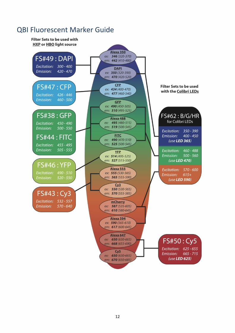
QBI Fluorescent Marker Guide
12