zambian smallholder behavioral responses to food reserve agency activities

FOOD SECURITY RESEARCH PROJECT

ZAMBIAN SMALLHOLDER BEHAVIORAL RESPONSES TO FOOD RESERVE AGENCY

ACTIVITIES

by

Nicole M. Mason, T. S. Jayne, and Robert J. Myers

WORKING PAPER No. 59 FOOD SECURITY RESEARCH PROJECT LUSAKA, ZAMBIA December 2011 (Downloadable at: http://www.aec.msu.edu/agecon/fs2/zambia/index.htm )

http://www.aec.msu.edu/agecon/fs2/zambia/index.htm

ii

ZAMBIAN SMALLHOLDER BEHAVIORAL RESPONSES TO FOOD

RESERVE AGENCY ACTIVITIES

by

Nicole M. Mason, T. S. Jayne, and Robert J. Myers

FSRP Working Paper No. 59

December 2011

Mason and Jayne are, respectively, assistant professor and professor, International Development, in the Department of Agricultural, Food, and Resource Economics at Michigan State University (AFRE/MSU) and currently on long-term assignment with the Food Security Research Project (FSRP) in Lusaka, Zambia. Myers is university distinguished professor in AFRE/MSU.

iii

ACKNOWLEDGMENTS The Food Security Research Project is a collaborative program of research, outreach, and local capacity building, between the Agricultural Consultative Forum, the Ministry of Agriculture and Cooperatives, and Michigan State University’s Department of Agricultural, Food, and Resource Economics. The authors are grateful to the Food Reserve Agency (FRA) for releasing detailed data on its maize purchases and to Antony Chapoto, Masiliso Sooka, Stephen Kabwe, Solomon Tembo, Nick Sitko, and Kasweka Chinyama for liaising with the FRA to obtain these data. They also wish to thank Jeff Wooldridge, David Mather and Jake Ricker-Gilbert for feedback on the paper; Milu Muyanga for input on the maize price prediction model; Margaret Beaver for technical assistance with the survey data used in the study; and Patricia Johannes for formatting and editorial assistance. The authors acknowledge financial support from the United States Agency for International Development Zambia Mission and the Bill and Melinda Gates Foundation. Any views expressed or remaining errors are solely the responsibility of the authors. Comments and questions should be directed to the Project Director, Food Security Research Project, 26A Middleway, Kabulonga, Lusaka; Tel +260 (21)1261194; email: [email protected].

mailto:[email protected]

iv

FOOD SECURITY RESEARCH PROJECT TEAM MEMBERS

The Zambia Food Security Research Project field research team is comprised of Chance Kabaghe, Antony Chapoto, T. S. Jayne, William Burke, Nicole Mason, Munguzwe Hichaambwa, Solomon Tembo, Stephen Kabwe, Auckland Kuteya, Nicholas Sitko, Mary Lubungu, and Arthur Shipekesa. MSU-based researchers in the Food Security Research Project are Steve Haggblade, James Shaffer, Margaret Beaver, David Tschirley, and Chewe Nkonde.

v

EXECUTIVE SUMMARY

More than two decades after the initiation of agricultural market reforms in eastern and southern Africa (ESA), governments in the region are increasingly using parastatal grain marketing boards (GMBs) and/or strategic grain reserves (SGRs) to directly influence the prices faced by farmers and consumers. In Zambia, for example, the government through the Food Reserve Agency, a SGR/GMB, purchased nearly 400,000 metric tons (MT) of maize from smallholders in 2006/07 and 2007/08, or more than 50% of the maize marketed by this group. This marked a sharp increase in the level of FRA purchases: between its establishment in 1996 and the 2005/06 marketing year, FRA’s annual maize purchases only once exceeded 100,000 MT. Then in 2010/11, the FRA purchased more than 80% of expected smallholder marketed maize (878,570 MT). The FRA buys maize at a pan-territorial price that often exceeds market price levels. Private trade is legal and private buyers are allowed to buy maize at prices above or below the FRA price. Significant public resources are devoted to the FRA. During budget years 2004 through 2011, the Agency’s budget allocation averaged 25% of the total allocation to Poverty Reduction Programmes (PRP) in Zambia. The vast majority of the remaining PRP funds were allocated to the main government fertilizer subsidy program, the Farmer Input Support Programme (formerly the Fertilizer Support Programme). Despite the re-emergence or continuation of GMBs/SGRs as important players in grain markets in ESA, little is known about how these agencies’ scaled-up activities are affecting fertilizer use and crop production by smallholder households. In this paper, we use nationally-representative household-level panel survey data from Zambia to estimate the marginal effects of the FRA’s maize purchase price and quantities purchased on smallholder behavior, while controlling for the effects of the Government of the Republic of Zambia (GRZ) fertilizer subsidy programs and other factors. The panel data cover the 1999/2000, 2002/03, and 2006/07 agricultural seasons, and therefore capture years before and during the recent scaling-up of the FRA’s activities. The smallholder behavioral responses examined are fertilizer demand (kilogram (kg) of fertilizer applied per hectare (ha) of maize) and crop output supply (total, maize, and non-maize area planted, crop output per hectare, and crop output). The empirical models are estimated in two stages. In the first stage, we estimate the marginal effects of FRA maize purchase and pricing policies on the mean and variance of farmgate maize market and FRA prices at the next harvest and on the probability that a household will sell to the Agency at the next harvest. Predicted values from the first stage regressions are used to construct an expected maize price for each household and agricultural year in the panel survey. The expected maize price is then included as an explanatory variable in the second stage fertilizer demand and output supply regressions. The empirical results point to three key findings. First, an increase in the volume of maize purchased by the FRA in a household’s district in previous years or an increase in the effective FRA maize price faced by the household at the previous harvest has a positive effect on the household’s expected maize price at the next harvest. A 1% increase in past FRA maize purchases increases households’ expected maize price in 2006/07 by 0.10%. The magnitude of this elasticity is larger for smallholders that cultivate two or more hectares of land or are located in areas that are well suited for low input rainfed maize production. The elasticity of the expected maize price with respect to the lagged effective FRA price is also positive and statistically significant (p<0.10) for these households.

vi

Second, an increase in the expected maize price has a positive effect on total and maize area planted, a negative effect on maize yields, and no statistically significant effect on the intensity of fertilizer use on maize, non-maize area planted, total and non-maize output per hectare, and total, maize, and non-maize output. The positive maize area effect and the negative maize yield effect offset each other, and as a result, there is no statistically significant change in maize quantity harvested. The negative marginal yield effect may be because the additional area planted to maize is of poorer quality or in areas that are agro-ecologically ill-suited for maize. Third, the first- and second-stage results combined show that for 2006/07, increases in past FRA district-level maize purchases and in the lagged effective FRA price are associated with:

• household-level increases in total and maize area planted, • a decrease in maize yield, and • no significant change in maize quantity harvested, total crop output, or the other

dimensions of smallholder behavior examined. Raising rural incomes, improving national food security, and stabilizing crop prices are core FRA objectives. Although we do not estimate the effects of past FRA behavior on food security or incomes per se, the finding of no statistically significant impact of FRA activities on maize or total crop output does not support the conclusion of improvement in food security or incomes. A large proportion of Zambia’s public resources are devoted to the FRA. For example, in the 2010/11 marketing season, spending on the FRA amounted to approximately 2% of the nation’s GDP. Between 2004 and 2011, GRZ allocated an average of 25% of its annual Poverty Reduction Programmes budget to the FRA. The failure of FRA policies to increase smallholder maize and total crop output, and the fact that it is mainly relatively well-off smallholders who benefit from the high FRA purchase price, calls into question the efficacy of maize price supports as a poverty reduction tool in Zambia. Indeed, at approximately 80%, rural poverty rates remain stubbornly high and there has been no substantive reduction in rural poverty since the FRA was established in 1996. GRZ and donor funds devoted to the FRA come at a high opportunity cost. Limiting FRA involvement in the maize market to securing the national strategic food reserve, its original mandate, would free up resources that could be invested in the known drivers of pro-poor agricultural growth such as agricultural research, development and extension, rural infrastructure, and education

vii

TABLE OF CONTENTS

ACKNOWLEDGMENTS ....................................................................................................... iii

EXECUTIVE SUMMARY ....................................................................................................... v

LIST OF TABLES ................................................................................................................. viii

ACRONYMS ............................................................................................................................ ix

1. INTRODUCTION ............................................................................................................... 1

2. THE FOOD RESERVE AGENCY ...................................................................................... 3

2.1. Overview of FRA Activities .......................................................................................3 2.2. Smallholder Maize Sales to FRA and Socioeconomic Characteristics of Sellers vs.

Non-Sellers .................................................................................................................5 3. DATA ................................................................................................................................... 6

4. METHODS ........................................................................................................................... 7

4.1. Conceptual Framework ...............................................................................................7 4.2. Empirical Models ........................................................................................................8 4.2.1. Expected Values for FRA and Private Sector Log Maize Prices ..................... 8 4.2.2. Variances for FRA and Private Sector Log Maize Prices ................................ 9 4.2.3. Covariance of FRA and Private Sector Log Maize Prices ............................. 10 4.2.4. The Probability that the FRA Channel Will Be Available at Harvest ........... 10 4.2.5. Expected Prices for Non-maize Crops, E( po ) ............................................. 10

4.2.6. Empirical Factor Demand and Output Supply Equations .............................. 11 5. RESULTS .......................................................................................................................... 13

5.1. Expected Maize Price Auxiliary Regressions and Marginal Effects of Past FRA Policies on a Household’s Expected Maize Price .....................................................13

5.2. Marginal Effects of the Expected Maize Price on Smallholder Behavior ................15 5.3. Marginal Effects of Past FRA Effective Prices and Purchases on Smallholder

Behavior ....................................................................................................................17 6. CONCLUSIONS AND POLICY IMPLICATIONS ......................................................... 19

APPENDICES ......................................................................................................................... 21

APPENDIX A: SUMMARY STATISTICS ........................................................................... 22

APPENDIX B: FULL REGRESSION RESULTS ................................................................. 26

REFERENCES ........................................................................................................................36

viii

LIST OF TABLES TABLE PAGE 1. FRA Maize Prices and Purchases, and Estimated Smallholder Maize Production and Sales, 1996/97-2010/11 Marketing Years .....................................................................4 2. Smallholder Socioeconomic Characteristics by Participation in FRA ................................5 3. Key Results from Log Effective Maize Price and Log Squared Residuals Regressions ...14 4. Key Results from CRE Probit: Hh Sold Maize to FRA at Harvest =1; =0 Otherwise ......14 5. Probability of Selling Maize to the FRA at the Next Harvest ...........................................15 6. Average Elasticities of Expected Maize Price W.R.T. Past FRA Effective Maize Price and District-Level Purchases .............................................................................................16 7. Average Partial Effects and Average Elasticities of Fertilizer Use on Maize and Output Supply W.R.T. the Expected Maize Price .............................................................16 8. Apes and AES of Total and Maize Area Planted and Maize Yield W.R.T. Past FRA

Policies, 2006/07 Agricultural Year ..................................................................................18 A.1. Summary Statistics for Continuous Explanatory Variables ............................................22 A.2. Summary Statistics for Binary Explanatory Variables ...................................................24 A.3. Summary Statistics for Dependent Variables .................................................................25 B.1. Results from Log Effective Market and FRA Maize Price and Log Squared Residuals Regressions .....................................................................................................26 B.2. CRE Probit Results: HH Sold Maize to FRA at Harvest =1; =0 Otherwise ...................29 B.3. Fertilizer Use on Maize (kg/ha) Regression Results .......................................................30 B.4. Total and Maize Area Planted (ha) Regression Results ...................................................32 B.5. Total, Maize, and Non-maize Output per Hectare Regression Results ...........................34

ix

ACRONYMS AE Average Elasticity AFRE/MSU Agricultural, Food, and Resource Economics at Michigan State University APE Average Partial Effect CFS Crop Forecast Survey CRE Correlated Random Effects CSO Central Statistical Office ESA Eastern and Southern Africa FE Fixed Effects FEWSNET Famine Early Warning Systems Network FIQI Fisher Ideal Quantity Index FISP Farmer Input Support Programme FRA Food Reserve Agency FSP Fertilizer Support Programme FSRP Food Security Research Project GMB Grain Marketing Board GRZ Government of the Republic of Zambia ha Hectare kg Kilogramme MACO Ministry of Agriculture and Cooperatives MT Metric Ton PHS Post-Harvest Survey POLS Pooled Ordinary Least Squares PRP Poverty Reduction Programme SGR Strategic Grain Reserve SS Supplemental Survey WFP World Food Programme ZMK/K Zambian Kwacha

1

1. INTRODUCTION

More than two decades after the initiation of agricultural market reforms in eastern and southern Africa (ESA), several governments in the region continue to be directly engaged in staple food marketing (Jayne and Jones, 1997; Jayne et al., 2002; Jayne, Chapoto, and Govereh 2007). While the recent re-introduction or scaling-up of fertilizer subsidy programs, particularly in Malawi, has received much attention in the popular press and from policy makers and researchers (see, for example, Denning et al. 2009; Duflo, Kremer, and Robinson 2009; Ricker-Gilbert, Jayne, and Chirwa 2011; Dugger 2007; Kapekele, 2010), governments in ESA are also increasingly using parastatal grain marketing boards (GMBs) and/or strategic grain reserves (SGRs) to directly influence the prices faced by farmers and consumers.1 Zambia is a key example. Not only has the GRZ since 2002/03 distributed large quantities of subsidized fertilizer to smallholders through its Fertilizer Support Programme/Farmer Input Support Programme (FSP/FISP), but it has also become the major buyer of smallholder maize in the country. During the 2006/07 and 2007/08 agricultural marketing years, the GRZ strategic food reserve/maize marketing board, the Food Reserve Agency (FRA), purchased nearly 400,000 MT of maize from smallholders, or more than 50% of the maize marketed by this group.2 This marked a sharp increase in the level of FRA purchases: between its establishment in 1996 and the 2005/06 marketing year, FRA’s annual maize purchases only once exceeded 100,000 MT. The FRA purchased 878,570 MT of maize or 83% of expected smallholder maize sales in 2010/11. The FRA buys maize at a pan-territorial price that often exceeds market price levels. Private trade is legal and private buyers are allowed to buy maize at prices above or below the FRA price. Together, FRA and FSP/FISP accounted for over 90% of the GRZ budget allocation to Poverty Reduction Programmes in budget years 2006 to 2011. Despite the re-emergence or continuation of GMBs/SGRs as important players in grain markets in ESA, little is known about how these agencies’ scaled-up activities are affecting fertilizer use and crop production by smallholder households. The literature on the impacts of GMBs in the region focuses mainly on the decades prior structural adjustment and on the effects of the dismantling or downsizing of these entities during the 1980s and 1990s (e.g., Jansen 1991; Krueger 1991; Schiff and Valdés 1991; Masters and Nuppenau 1993; Krueger 1996). This paper revisits the impacts of GMBs/SGRs on smallholder behavior in light of recent events, modern conditions, and new, more detailed and disaggregated data. More specifically, we use nationally-representative household-level panel survey data from Zambia to estimate the marginal effects of the FRA’s past maize purchase price and quantities purchased on smallholder behavior, while controlling for the effects of GRZ fertilizer subsidy programs and other factors. The panel data cover the 1999/2000, 2002/03, and 2006/07 agricultural seasons, and therefore capture years before and during the recent

1 A marketing board is a state-controlled or state-sanctioned entity established to direct the market and marketing of specific commodities within a given country or other geographic area (Staatz 2006; Barrett and Mutambatsere 2008). A strategic grain reserve is a “public stock of grain used to meet emergency food requirements, to stabilize food prices, and [or] to relieve temporary shortages while commercial imports or food aid are being arranged” (Minot 2010). Some entities that refer to themselves as SGRs, e.g., the Zambian Food Reserve Agency, have functions such as grain marketing and market facilitation that are more characteristic of GMBs. 2 Smallholder households are those cultivating less than 20 ha. The agricultural marketing year in Zambia, henceforth referred to as marketing year, is from May to April. The agricultural year is from October through September.

2

scale-up of FRA maize purchases. In addition to measuring the marginal effects of changes in FRA domestic maize purchase policies on smallholder fertilizer use on maize, crop area planted, output per hectare, and output, the paper’s other main objective is to identify the policy implications of the findings. The remainder of the paper is organized as follows. Section 2 is an overview of FRA activities with particular emphasis on the Agency’s domestic maize purchases during the 1996/97-2007/08 marketing years. Sections 3 and 4 describe the data and methods, respectively. Results are presented in section 5, and the conclusions and policy implications are discussed in section 6.

3

2. THE FOOD RESERVE AGENCY

2.1. Overview of FRA Activities

The FRA, a parastatal, was established in 1996 with the enactment of the Food Reserve Act of 1995. The FRA’s original primary function was to establish and administer a national food reserve and the Agency was to be involved in crop marketing only as necessary to perform this function (GRZ 1995). Crop marketing and market facilitation were officially added as FRA functions when the Food Reserve Act was amended in 2005 (GRZ 2005). Raising rural incomes, improving national food security, and stabilizing crop prices are core FRA objectives (FRA n.d.). Maize is the most important crop in Zambia and the Agency’s emphasis has been almost exclusively on maize. For example, in the 2005/06 marketing year, 95% of the FRA’s budget for crop purchases was for maize (FRA 2005). The household panel survey data used in this paper cover the 1999/2000, 2002/03, and 2006/07 agricultural years and subsequent marketing years (2000/01, 2003/04, and 2007/08). Table 1 summarizes FRA domestic maize purchase activities during the 1996/97 through 2010/11 marketing years. During its first two years in operation (1996/97 and 1997/98), the FRA contracted small-scale traders to buy maize from smallholders on its behalf. The quantities purchased were small and only made in four to five districts. The price paid by the Agency to contracted traders varied across districts to reflect different market conditions3. The FRA did not purchase maize in Zambia from 1998/99 to 2001/02 due to lack of funding. Therefore, at planting time in the 1999/2000 agricultural year (captured in the first wave of the panel survey), the FRA had not purchased maize in Zambia in two years and had no plans to do so for the foreseeable future.4 In July 2002 following drought-related poor harvests in many areas of Zambia, GRZ allocated K12 billion to the FRA to buy 15,000 MT of maize directly from smallholders in eight surplus districts (FEWSNET and WFP 2002). Sourcing maize directly from smallholders rather than through private traders marked a distinct change in FRA procurement practices.5 By the end of October 2002, the FRA had purchased 9,059 MT in eight districts. The Agency continued buying maize through March 2003 and purchases for the 2002/03 marketing year totaled 23,535 MT from 10 districts. Thus, at planting time in the 2002/03 agricultural year (captured in the second wave of the panel survey), the FRA was buying maize directly from smallholders for the first time since its establishment but only in eight of Zambia’s 72 districts. In May 2003, the FRA announced its 2003/04 marketing year plans to purchase 205,700 MT of maize directly from smallholders in 37 districts at a pan-territorial price of K30,000 per 50-kg bag. This was the first time since 1992 that GRZ announced a pan-territorial price for maize (FEWSNET 2003a; FEWSNET 2003b). The Agency ultimately only purchased 54,847 MT (15-19% of smallholder maize sales) due to funding shortfalls but its ambitious purchase target signaled its intention to become a major player in the Zambian maize market.

3 Chance Kabaghe. Personal communication, 5 March 2010. 4 Here and throughout the rest of the paper, we use planting time as shorthand for the period during which households make land preparation, fertilizer use, and planting decisions. 5 In order to sell to the FRA, smallholders are required to be members of a cooperative or other farmer group (FRA various years). Smallholder sellers deliver their maize to satellite depots set up by the FRA in targeted districts and are to be paid within ten days, although payment delays are common.

4

Table 1. FRA Maize Prices and Purchases, and Estimated Smallholder Maize Production and Sales, 1996/97-2010/11 Marketing Years

Marketing year

FRA pan- territorial

price (ZMK*/50

kg)

# of districts with FRA

maize purchasesd

FRA domestic

maize purchases

(MT)

Estimated smallholder maize:e

FRA purchases as % of

smallholder maize sales

Production and sales

data source

Production (MT)

Sales (MT)

1996/1997 11,800a 5 10,500 1,117,955 280,955 3.7 PHS 1997/1998 7,880a 4 4,989 804,626 206,557 2.4 PHS 1998/1999 N/A 0 0 724,024 175,515 0 PHS 1999/2000 N/A 0 0 929,304 242,753 0 PHS 2000/2001 N/A 0 0 1,253,722 303,738 0 PHS 1,282,352 323,387 0 SS 2001/2002 N/A 0 0 957,437 209,326 0 CFS 938,539 197,915 0 PHS 2002/2003 40,000b 10 23,535 673,673 143,453 16.4 CFS 947,825 195,407 12.0 PHS 2003/2004 30,000 36 54,847 970,317 260,885 21.0 CFS 1,126,316 291,462 18.8 PHS 1,365,538 370,332 14.8 SS 2004/2005 36,000 46 105,279 1,364,841 331,006 31.8 CFS 1,216,943 356,750 29.5 PHS 2005/2006 36,000 50 78,667 652,414 151,514 51.9 CFS 800,574 206,092 38.2 PHS 2006/2007 38,000 53 389,510 1,339,479 454,676 85.7 CFS 1,388,311 674,020 57.8 PHS 2007/2008 38,000 58 396,450 1,419,545 533,632 74.3 CFS 1,960,692 762,093 52.0 SS 2008/2009 45,000c 58 73,876 1,392,180 522,033 14.2 CFS 2009/2010 65,000 59 198,630 1,657,117 613,356 32.4 CFS 2010/2011 65,000 62 878,570 2,463,523 1,062,010 82.7 CFS Sources: FRA; MACO/CSO Crop Forecast Surveys (CFS); MACO/CSO Post-Harvest Surveys (PHS); CSO/MACO/FSRP Supplemental Surveys (SS). * Zambian Kwacha Notes: aNot a pan-territorial price but the average price paid by FRA to private traders, who procured from smallholders. bNot a pan-territorial price but the price paid by FRA directly to smallholder farmers in the districts where it was purchasing; initial FRA price of K30,000 was raised to K40,000 in August 2002. cFRA price increased to 55,000 in September 2008. dThere are 72 districts in Zambia. eSmallholder maize production and sales based on CFS data are expected, not realized, levels.

The FRA increased its market share in 2004/05 and 2005/06, accounting for 30% and 38% of smallholder maize sales, respectively (Table 1). At harvest time in 2006, the FRA planned to purchase 80,000 MT of maize in 55 districts at K38,000 per bag. Following a surge of sales from smallholders, in July the Agency increased its purchase target to 200,000 MT. By the time buying ended on September 30, 2006 (two days after presidential and parliamentary elections), FRA purchases totaled nearly 360,000 MT. The Agency re-entered the market in November and December, and total FRA purchases for 2006/07 were 389,510 MT (58% of smallholder maize sales). Therefore, at planting time in the 2006/07 agricultural year (captured in the third wave of the panel survey), the FRA was the dominant buyer of smallholder maize in Zambia and had purchased maize directly from smallholders in five consecutive years. At K38,000 per 50-kg bag, the FRA 2006/07 buy price was well above wholesale maize market prices, which ranged from K23,000 to K31,000. The Agency’s buying presence had increased from 10

5

districts in 2002/03 to 53 districts in 2006/07. The FRA purchased nearly 400,000 MT again in 2007/08.6 2.2. Smallholder Maize Sales to FRA and Socioeconomic Characteristics of Sellers vs. Non-Sellers

The FRA did not buy maize in Zambia during the marketing year captured by the first wave of the panel survey (2000/01) but it did purchase maize during the marketing years captured in the second and third waves (2003/04 and 2007/08). Table 2 summarizes the rate and level of smallholder participation in selling maize to the FRA in these two years and contrasts the socioeconomic characteristics of sellers and non-sellers. Less than 1% of smallholder households sold maize to the Agency in 2003/04. This percentage rose to nearly 10% in 2007/08 as the FRA scaled up its activities. In 2007/08, participating households sold an average of 2.76 MT to the FRA (1.25 MT at the median). Households that sold maize to the Agency had considerably larger landholdings, more farm assets, and heads with higher educational attainment, and were less likely to be female-headed than households that did not (Table 2). Table 2. Smallholder Socioeconomic Characteristics by Participation in FRA

Marketing year

Sold maize to FRA? Descriptive result Yes No Share of smallholder households 2003/2004 0.8% 99.2%

2007/2008 9.7% 90.3% Mean kg of maize sold to FRA 2003/2004 2,315 0 2007/2008 2,764 0 Median kg of maize sold to FRA 2003/2004 600 0 2007/2008 1,250 0 Mean landholding size (ha) 2003/2004 3.65 2.11 2007/2008 3.65 1.84 Mean value of farm assets 2003/2004 59.4 23.1 (100,000 ZMK, 2007/08=100) 2007/2008 65.7 18.8

Share female-headed 2003/2004 8.6% 21.9% 2007/2008 14.0% 25.0% Median education of HH head 2003/2004 8 5

(highest grade completed) 2007/2008 7 5 Sources: CSO/MACO/FSRP 2004 and 2008 Supplemental Surveys Notes: Farm assets are plows, harrows, and ox carts.

6 See Mason (2011, Appendix F) for additional details on the FRA and for information on GRZ fertilizer subsidy programs.

6

3. DATA

The data used in this paper are drawn mainly from a three-wave, nationally representative longitudinal survey of rural smallholder households in Zambia. The first wave was done in two parts: the 1999/2000 Post-Harvest Survey (PHS9900) conducted by the Zambian Central Statistical Office (CSO) and Ministry of Agriculture and Cooperatives (MACO) in August-September 2000, and the linked CSO/MACO/FSRP (Food Security Research Project) Supplemental Survey conducted in May 2001 (SS01). The second and third waves were the Supplemental Surveys (SS) conducted in May 2004 (SS04) and June-July 2008 (SS08). PHS9900 and SS01 covered the 1999/2000 agricultural year and 2000/01 marketing year. A total of 7,699 rural households from 70 districts were interviewed for PHS9900. Households were selected using a stratified three-stage sampling design. See Megill (2005) for details. PHS9900 focused on households’ agricultural activities. For SS01, attempts were made to revisit all PHS9900 households to collect information on household demographics, off-farm income and remittances, and other details. 6,922 of the 7,699 PHS9900 households were successfully re-interviewed in SS01 (89.9% re-interview rate). A second attempt was made to revisit PHS9900 households for SS04, which covered the 2002/03 agricultural year and 2003/04 marketing year. SS04 included questions comparable to those on PHS9900 and SS01 plus additional questions. 5,358 SS01 households were successfully re-interviewed (77.4% re-interview rate). The third re-interview of PHS9900 households was SS08, which covered the 2006/07 agricultural year and 2007/08 marketing year. SS08 questions mirrored SS04 and 4,286 SS04 households were successfully revisited (a re-interview rate of 80.0%). Unless otherwise noted, we use the unbalanced panel of households that were interviewed in at least SS01 and SS04, if not SS08. Given non-trivial attrition rates between rounds of the SS, attrition bias is a potential problem. However, tests for attrition bias as described in Wooldridge (2002: p. 585) fail to reject the null hypothesis of no attrition bias in all cases (0.20 < p < 0.85). Other data used in the study are: (i) FRA administrative records on yearly district-level maize purchases from 1996/97 to 2006/07; (ii) dekad (10-day period) rainfall data covering the 1990/91 to 2006/07 growing seasons and collected from 36 stations throughout Zambia by the Zambia Meteorological Department; (iii) crop prices from MACO/CSO Post-Harvest Surveys for 1998/99, 2001/02, and 2005/06; (iv) constituency-level data on the percentage of votes won by the ruling party and opposition parties during the 1996, 2001, and 2006 presidential elections from the Electoral Commission of Zambia; and (v) monthly maize wholesale prices from trading centers in each of Zambia’s nine provinces from MACO’s Agriculture Market Information Center.

7

4. METHODS For a detailed discussion of the conceptual framework, empirical models, and estimation strategy used in the paper, see Mason (2011, Chapter 2). In this section, we provide an overview of the methodology.

4.1. Conceptual Framework

In modeling the marginal effects of the FRA’s maize pricing and purchases on smallholder fertilizer demand and crop output supply, four key features of the decision-making environment need to be taken into consideration. First, at planting time farmers do not know the price at which the FRA will buy maize and the prices at which private traders will buy maize and other crops at the next harvest. Second, households do not know if the FRA will be buying maize in their area during the next marketing year. Third, the FRA pan-territorial buy price is not a floor price. Private sector buyers can legally buy maize for more or less. Fourth, the effective FRA price (i.e., the FRA pan-territorial price adjusted for transfer costs from the homestead to an FRA satellite depot) varies across households. Several key assumptions are made en route to deriving fertilizer demand and output supply functions. First, assume that the agricultural producer in question is risk-neutral and maximizes expected profit. Second, suppose there is a single (private sector) marketing channel for non-maize crops and that there are two potential marketing channels for maize: private sector and FRA. Third, assume that the household sells maize to only one marketing channel – the one with the higher effective price. 7 Fourth, assume that the private sector channel is always available but the FRA channel is available at harvest with probability E(γ ) , which is between zero and one and is unknown to the farmer at planting time. (E(.) is the expectations operator.) Let

p f , pp , and po be, respectively, the effective FRA and

private sector maize prices and a vector of other crop prices at the next harvest. These prices are unobserved to the farmer at planting time. Fifth, assume that variable input prices ( w) are known at planting time, and let z be a vector of production shifters. Under these assumptions, a representative household’s fertilizer demand or crop output supply function (y) is:

y = y p*,E( po),w;z⎡⎣⎢

⎤⎦⎥ (1)

where

p* ≡ E(γ )E[max( p f , pp )]+ [1− E(γ )]E( pp ), (2)

is the expected (effective) maize price.8 Equation (2) shows that the expected maize price is a weighted average of the expected maximum of maize prices in the FRA and market channels, E[max( p f , pp )] , and the expected private sector price, E( pp ) . The weights on these two

prices are a function of the probability that the FRA channel will be available to the

7 This is consistent with household survey evidence from Zambia. In the 2007/08 and 2009/10 marketing years, only 5% of maize-selling smallholder households sold maize to both private sector buyers and the FRA. More than 80% of maize-selling smallholder households had only one maize sale transaction. 8 The additional assumptions that γ is independent of p f and pp but that p f and pp are not independent

are also required.

8

household at the next harvest, E(γ ) . Note that if the FRA channel will definitely not be available, i.e., E(γ ) = 0 , then the expected maize price is simply the expected private sector price. Conversely, if the FRA channel will definitely be available, the expected maize price is the expected maximum of prices in the two marketing channels. To further evaluate E[max( p f , pp )] , we need to make an assumption about the joint distribution of

p f and

pp . We assume bivariate log normality as an approximation. Under this assumption,

E[max( p f , pp )] is a function of the means, variances, and covariance of the natural logs

(ln) of the two prices (Lien 2005). In the empirical application, the challenge is to first measure these means, variances, and covariance, as well as the probability that the FRA channel will be available at the next harvest. Past FRA domestic maize purchases and prices are hypothesized to influence these values. Next, an expected maize price, p*, is constructed per equation (2) and we can measure the marginal effects of past FRA policies on a household’s expected maize price. Then, the expected maize price is included as an explanatory variable in the household’s fertilizer demand or output supply function per equation (1). From this equation, we can measure the marginal effect of the expected maize price on household behavior. Finally, we take the product of these two marginal effects ((i) the marginal effect of FRA policies on the expected maize price, and (ii) the marginal effect of the expected maize price on household behavior) to obtain an estimate of the marginal effect of FRA policies on smallholder behavior. 4.2. Empirical Models

In the sub-sections that follow, we first describe how we estimate households’ subjective means, variance, and covariance of harvest-time prices in the FRA and private sector maize marketing channels, and households’ subjective probabilities that the FRA channel will be available to them come harvest time. The general approach is to regress, for example, the farmgate FRA price received by households that sold to the Agency at the next harvest on variables observed by all households at planting time and hypothesized to influence the maize price they receive and their price expectations. These variables include FRA policies during the previous marketing year. We then use the regression results to compute predicted farmgate FRA prices at the next harvest for all households in the sample, regardless of if they ultimately sold to FRA at the subsequent harvest or not. Next, we specify the empirical fertilizer demand and crop output supply equations and describe how these equations are estimated. Readers not interested in the details of the empirical models and estimation strategy used in the study may wish to skip to the Results (section 5). 4.2.1. Expected Values for FRA and Private Sector Log Maize Prices Estimates of a household’s subjective expected values for log effective maize prices in the FRA and market channels ( E(ln p j ) = μ j , j = f , p ) are obtained by first estimating

(3)

9

where p j, i,t is the effective channel j maize price received by household i in harvest year t

(the price at the point of sale minus estimated transportation costs from the homestead/farm to the point of sale); Ωi,t−1 is a vector of information observed by the household at planting

time and hypothesized to influence the maize price it receives and inform its expectation of harvest time maize prices; is a vector of parameters to be estimated; ci is time invariant

household-level unobserved heterogeneity; and ε j,i,t is the error term. Ωi,t−1 includes,

among other things, maize prices in the two marketing channels at the previous harvest, and the volume of maize purchased by the FRA in the household’s district in the previous marketing year(s). See Tables A.1 and A.2 in Appendix A for a list of the variables included in Ωi,t−1 and associated summary statistics.

Equation (3) is estimated by correlated random effects-pooled ordinary least squares (CRE-POLS) using data from households that sold maize to marketing channel j and for which the effective maize price received can be estimated from the SS data.9 See Wooldridge (2002) for details on the CRE approach. This estimator is used because it allows us to control for time invariant unobserved household effects ( ci) that may be correlated with the explanatory

variables in equation (3). If not controlled for, ci can render inconsistent the estimates of the parameters in the equation. Because the variables in Ωi,t−1 are observed for all households whether or not they sold

maize to marketing channel j, once estimated, equation (3) can be used to obtain predicted values for all households in the sample. These predicted values are used as households’ subjective values for expected log maize prices in the two marketing channels.10

4.2.2. Variances for FRA and Private Sector Log Maize Prices The (conditional) variance of the log maize price in marketing channel j is equal to the expected value of the squared error term in equation (3). We estimate this expected value using an approach similar to the one described in the previous section. We first regress the log squared residuals from equation (3) on Ωi,t−1, the vector of information observed by the

household at planting time and hypothesized to influence its maize price expectations:

(4)

v j,i,t is the error term. Equation (4) is estimated using CRE-POLS and observations for

households that sold maize to marketing channel j. Then the estimated equation is used to

obtain predicted values ε j, i,t2 for all households in the sample. These predicted values are

9 Insufficient information was collected in SS01 to calculate effective maize prices, hence maize prices at the point of sale are used for that year. 10 Predicted log maize prices obtained for all smallholder households from parameter estimates based on data for those that sold maize to marketing channel j could therefore be plagued by selection bias. However, tests as described in Wooldridge (2002) fail to reject the null hypothesis of no sample selection bias in all cases for the expected values and variances of maize prices in the two marketing channels.

10

used as households’ subjective values for the variance of the log maize prices in the two channels.

4.2.3. Covariance of FRA and Private Sector Log Maize Prices The (conditional) covariance of the effective log maize prices in the two channels is a function of the (conditional) variances and correlation coefficient (ρ ) of these prices:

Cov(ln p f ,ln pp ) = ρ Var(ln p f ) Var(ln pp ) (5)

We assume that the correlation coefficient is a constant and estimate it as the sample correlation between

ε f , i,t and

ε p, i,t (the residuals from the log effective maize price

equations for households that sold to both the FRA and private buyers in year t). The household’s subjective covariance is then calculated per equation (5) using this correlation coefficient and the household’s subjective variance estimates. 4.2.4. The Probability that the FRA Channel Will Be Available at Harvest SS04 and SS08 did not ask respondents if the FRA channel was available in their area during the 2003/04 and 2007/08 marketing years, respectively, but we do know if a given household sold maize to the FRA in these years. In the empirical application, γ i,t = 1 if the household

sold maize to the FRA, and zero otherwise. A household’s subjective probability that γ i,t = 1 is defined as the predicted probability from the probit model:

(6)

where is a vector of parameters to be estimated. Equation (6) is estimated by CRE probit. All 1999/2000 households and 2002/03 households outside of the eight districts where the FRA had purchased maize as of planting time in 2002 are excluded from the probit and assigned zero probability of selling to the FRA at the next harvest. Given the estimates of the expected values, variances, and covariance of log effective maize prices in the FRA and private sector channels, as well as the estimated probability that a

household will sell to the FRA at the next harvest, an expected maize price, pi,t* , can be

constructed for each household and agricultural year per equation (2). 4.2.5. Expected Prices for Non-maize Crops, E( po )

Non-maize crop prices in harvest year t-1 are used as proxies for expected year t prices. The commonly marketed crops for which lagged prices are available are groundnuts, mixed beans, and sweet potato.

11

4.2.6. Empirical Factor Demand and Output Supply Equations The empirical factor demand and output supply equations analogous to equation (1) are:

(7)

where pi,t* is the expected maize price (ZMK/kg); po,k,t -1 is a vector of median

groundnut, mixed bean, and sweet potato prices in province k at the previous harvest in ZMK/kg; wi,t is the effective fertilizer market price in ZMK/kg paid by households that

purchased fertilizer from commercial sources and the district median effective fertilizer market price otherwise; zi,t is a vector of other production shifters such as quasi-fixed

factors of production, rainfall, and household characteristics affecting production; govtferti,t

is the kilograms of government-subsidized fertilizer acquired by the household; ci is time

invariant household-level unobserved heterogeneity; and ui,t is the error term. Price data on

variable inputs other than fertilizer are not available. See Tables A.1 and A.2 in Appendix A for summary statistics for the explanatory variables in equation (7). A factor demand equation is estimated for the intensity of fertilizer use on maize (kg/ha). Output supply equations are estimated for area planted and crop output per hectare. Since crop output is equal to area planted times yield, we apply the product rule to estimation results for area planted and crop output per hectare to compute the average partial effects of key variables of interest on crop output, rather than estimating a separate equation for crop output. Equations are estimated for total, maize, and non-maize output per hectare. For area planted, equations are estimated for total area and maize area, and then partial effects on non-maize area are calculated as the difference of the partial effects on total area and maize area. Total refers to maize and the 16 non-maize crops covered by all three SSs: cassava, sweet potato, sorghum, millet, groundnut, mixed bean, cotton, rice, sunflower, soyabean, Irish potato, ground bean, cowpea, velvet bean, tobacco, and coffee. Total crop output and non-maize crop output are Fisher-Ideal Quantity Indexes (FIQI) (Diewert 1992; Diewert 1993). (See Mason (2011, Appendix B) for details.) Total and non-maize crop output per hectare are defined as the associated crop output FIQI divided by hectares planted to the crops included in the FIQI. See Table A.3 in Appendix A for summary statistics for the various dependent variables. Fixed effects (FE) is used to estimate equation (7) for all dependent variables. Like CRE, FE controls for unobserved time invariant household effects that may be correlated with the explanatory variables in equation (7). Fertilizer use on maize and maize area planted are equal to zero for 64% and 20% of the observations in the analytical sample, respectively. Given these pile-ups at zero, a Tobit estimator might better characterize the full distributions of fertilizer use on maize and maize area planted. Therefore, CRE Tobit is also used to estimate equation (7) for these variables. See Wooldridge (2002) for additional information on the Tobit estimator. FE and the CRE approach require that the explanatory variables in a regression be strictly exogenous. However, the quantity of government-subsidized fertilizer acquired by the household, govtferti,t , may be endogenous in equation (7). If it is, then all estimates of the

12

parameters in the equation may be inconsistent. To test and correct for the potential endogeneity of govtferti,t , we follow the approach in Ricker-Gilbert, Jayne, and Chirwa

(2011). See that paper and Mason (2011, Chapter 2) for details.

13

5. RESULTS

Sections 5.1. through 5.3. highlight the key findings of the analysis. In section 5.1., we discuss the results of the auxiliary regressions used to construct the expected maize price variable as well as the average partial effects (APEs) of the effective FRA maize price and district-level purchases on a household’s expected maize price. In section 5.2., we report the estimated APEs of the expected maize price on fertilizer use on maize and crop output supply. In section 5.3., we present the estimated APEs of past FRA policies on smallholder behavior. 5.1. Expected Maize Price Auxiliary Regressions and Marginal Effects of Past FRA Policies on a Household’s Expected Maize Price

Table 3 reports the key results of interest from the log effective FRA and market maize price regressions and those for the associated log squared residuals per equations (3) and (4). See Table B.1 in Appendix B for the full regression results. Larger FRA district-level maize purchases at the previous harvest are associated with a higher effective maize market price at the upcoming harvest (Table 3, row A). For each additional 10,000 MT purchased by the FRA in a household’s district, the harvest-time effective market price is expected to increase by 6.67% (p=0.024). This is consistent with a priori expectations. Once the FRA begins buying maize in a district, it generally returns to that district to buy maize in subsequent years. Higher FRA purchases in a given area are expected to put upward pressure on market prices there. Holding past FRA purchases in the household’s district constant, the lagged FRA farmgate maize price has no statistically significant effect on the harvest-time maize market price (p>0.10). This may be because the FRA farmgate price is in large part determined by the FRA pan-territorial price. Changes over time in the pan-territorial price and other national-level policies and conditions are captured by the year dummies in the model. 11 The elasticity of the harvest time FRA price with respect to the lagged FRA price is 0.341 and significant at the 1% level (Table 3, row C). This result is consistent with the fact that it has proven difficult politically for the FRA to lower its pan-territorial buy price from one year to the next. In fact, the FRA price has either increased or stayed the same every year since it began setting a pan-territorial price in 2003/04. So higher FRA prices in one year lead to the expectation of higher FRA prices the following year. The partial effect of past FRA purchases in the household’s district on the harvest time FRA price is not statistically different from zero at the 10% level. This suggests that expectations of future FRA prices are driven primarily by past FRA prices and not by the level of FRA activity in the district. This is reasonable since FRA pricing is pan-territorial. Both the level and square of district-level FRA maize purchases during the previous harvest are statistically significant at the 5% level in the equation for the variance of maize market prices. The coefficient on the level term is negative while the coefficient on the squared term is positive (Table 3, row B).

11 An interaction term is included in the regressions reported in rows A and B of Table 3 to allow the effect of the FRA price variable to differ in 1999/2000 versus 2002/03 and 2006/07. The Agency did not buy maize in Zambia in 1999/2000 so there is no FRA price that year and the effective FRA price is set equal to the market price.

14

Table 3. Key Results from Log Effective Maize Price and Log Squared Residuals Regressions Key Explanatory Variables of Interest

Dependent variable

FRA district- level

purchases (‘000MT, t-1)

FRA district- level

purchases, squared

Log effective

FRA maize price (t-1)

Log effective FRA maize

price (t-1) × 1999/2000

(A) Log effective maize market price at harvest Coefficient 6.67E-03 -0.0221 0.417 p-value 0.024 0.811 0.056 (B) Log squared residuals from (A) Coefficient -0.149 4.85E-03 1.116 0.0469 p-value 0.007 0.033 0.101 0.989 (C) Log effective FRA maize price at harvest Coefficient -2.06E-03 0.341 p-value 0.373 0.000 (D) Log squared residuals from (C) Coefficient 0.0153 -4.021 p-value 0.825 0.074 Note: Standard errors computed using complex survey weights and Huber-White robust variance matrix estimator. Together, these results suggest that past FRA maize purchases have a negative partial effect on the variance of maize market prices at volumes below 15,330 MT. At 9,890 MT, the 90th percentile of lagged FRA purchases over the three waves of the panel survey is well below this level. Larger FRA purchases in a given area are therefore associated with less variable maize market prices. In general, these findings are consistent with time series analyses for Zambia and Kenya, which indicate that GMB activities in the two countries have raised and stabilized maize market prices (Jayne, Myers, and Nyoro 2008; Mason and Myers 2011). Key APEs from the probit to obtain a household’s predicted probability of selling maize to the FRA at the next harvest are reported in Table 4. See Table B.2 in Appendix B for the full regression results. A 1% increase in the previous year’s effective FRA price is associated with a small increase (0.003) in the probability that the household will sell to the FRA the following year (where probability ∈[0,1]). The long-run APE of a 1,000 MT increase in past FRA district-level purchases is a 0.032 increase in the probability that the household sells to Agency at the next harvest. As shown in Table 5, the actual and predicted probabilities of selling to the FRA at the next harvest are extremely low for the vast majority of smallholders. Table 4. Key Results from CRE Probit: HH Sold Maize to FRA at Harvest =1; =0 Otherwise Explanatory variables APE p-val. FRA district-level purchases (‘000 MT, t-1) 0.00303 0.427 FRA district-level purchases (‘000 MT, t-2) 0.0146 0.158 FRA district-level purchases (‘000 MT, t-3) -0.00670 0.703 FRA district-level purchases (‘000 MT, t-4) 0.00784 0.764 FRA district-level purchases (‘000 MT, t-5) 0.0128 0.214 Log effective FRA maize price (t-1) 0.279 0.003 Joint significance of lagged FRA district-level purchases (F-stat.) 3.77 0.003 Long-run effect of FRA district-level purchases (‘000 MT) 0.0315 0.058 Note: Standard errors computed using complex survey weights and Huber-White robust variance matrix estimator.

15

Table 5. Probability of Selling Maize to the FRA at the Next Harvest Predicted

probabilities from probit

Probabilities for all sample HHs

Summary statistic 2002/03 2006/07 N 5,441 5,358 4,286 Mean 0.0796 0.00333 0.0969 Std. deviation 0.126 0.0172 0.136 Percentile:

1st 8.19E-6 0 7.55E-6 5th 0.0000945 0 0.000139 10th 0.000414 0 0.00141 25th 0.00464 0 0.0110 50th 0.0289 0 0.0445 75th 0.0977 0 0.123 90th 0.226 0.00395 0.262 95th 0.343 0.0159 0.386 99th 0.621 0.0751 0.664

Observed mean 0.0799 0.00761 0.0971 Average elasticities (AE) of a household’s expected maize price with respect to an increase in past FRA district-level purchases and in the lagged effective FRA price are summarized in Table 6. In 2006/07, the AE with respect to past FRA district-level purchases is 0.103 (p=0.060). This means that a household’s expected maize price increases by 0.103% when lagged FRA maize purchases increase by 1%. In contrast, in 2002/03 the AE of the expected maize price with respect to past FRA purchases is not statistically different from zero. This is expected given that 75% of households had zero probability of selling to the FRA and a 99th percentile of 0.075 in that year (Table 5). The AE of the expected maize price with respect to past FRA district-level purchases is positive and statistically significant in 2006/07 overall and for all sub-groups examined. The relative size of the AEs is consistent with a priori expectations: it is larger among households that cultivate more land and in areas that are more suitable for low-input management rainfed maize production. Households in these two groups also have a positive and statistically significant AE of the expected maize price with respect to the lagged effective FRA maize price (Table 6). In summary, results suggest that an increase in past FRA district-level maize purchases and, for certain groups of households, an increase in the lagged effective FRA price are associated with statistically significant increases in the household’s expected maize price. 5.2. Marginal Effects of the Expected Maize Price on Smallholder Behavior

APEs and AEs of fertilizer use on maize and crop output supply with respect to the expected maize price are summarized in Table 7. The full regression results are reported in Tables B.3 to B.5 in Appendix B. Contrary to a priori expectations, an increase in the expected maize price has no statistically significant impact on maize quantity harvested (rows L and M). The APE of the expected maize price is statistically significant and positive for maize area planted (rows D and E) but negative for maize yield (row I). The area and yield effects offset each other, the result being no significant change in maize quantity harvested. The APE of the expected maize price on the intensity of fertilizer use on maize (kg/ha) is not statistically

16

different from zero (rows A and B). This result coupled with the positive APE on maize area planted suggests that an increase in the expected maize price is associated with an increase in total fertilizer use on maize (kg). Table 6. Average Elasticities of Expected Maize Price W.R.T. Past FRA Effective Maize Price and District-Level Purchases Average elasticity (AE) of expected maize price w.r.t.: FRA district-level purchases (t-1 to t-5) Effective FRA maize price (t-1) 2002/03 & 2006/07 ----2006/07 only---- 2002/03 & 2006/07 ----2006/07 only---- Population AE p-val. AE p-val. AE p-val. AE p-val. All households 0.0456 0.062 0.103 0.060 0.0991 0.130 0.121 0.160 Farm size category:

< 2 ha cultivated 0.0352 0.067 0.0796 0.064 0.0872 0.212 0.0962 0.353 >= 2 ha cultivated 0.0749 0.071 0.170 0.070 0.133 0.035 0.191 0.002

Suitability of area for low input management, rainfed maize: High/moderate 0.0569 0.072 0.128 0.070 0.102 0.059 0.130 0.004

Marginal/unsuitable 0.0311 0.071 0.0710 0.068 0.0961 0.327 0.109 0.532 Agricultural year:

2002/2003 -1.82E-4 0.861 0.0819 0.249 2006/2007 0.103 0.060 0.121 0.160

Notes: p-values based on 500 bootstrap replications. Results in bold are statistically significant at the 10% level. Table 7. Average Partial Effects and Average Elasticities of Fertilizer Use on Maize and Output Supply W.R.T. the Expected Maize Price Row Outcome variable Estimator APE AE p-value A Fertilizer use on maize (kg/ha) FE 0.000230 0.000847 0.995 B Fertilizer use on maize (kg/ha) CRE Tobit 0.0102 0.0509 0.817 C Total area planted (ha) FE 0.00148 0.843 0.063 D Maize area planted (ha) FE 0.000881 0.970 0.044 E Maize area planted (ha) CRE Tobit 0.000626 0.639 0.063 F Non-maize area planted (ha) Derived (C-D) 0.000595 0.615 0.158 G Non-maize area planted (ha) Derived (C-E) 0.000850 0.884 0.094a H Total output/ha (FIQI/ha) FE -0.000842 -0.037 0.897 I Maize yield (kg/ha) FE -1.388 -0.866 0.007 J Non-maize output/ha (FIQI/ha) FE 0.0114 0.516 0.327 K Total output (FIQI) Derived [f(C,H)] 0.0298 0.783 0.134 L Maize output (kg) Derived [f(D,I)] 0.0573 0.096 0.935 M Maize output (kg) Derived [f(E,I)] -0.229 -0.232 0.715 N Non-maize output (FIQI) Derived [f(F,J)] 0.0259 1.106 0.123 O Non-maize output (FIQI) Derived [f(G,J)] 0.0328 1.359 0.080b Notes: Results in bold are statistically significant at the 10% level. p-values based on 500 bootstrap replications. aNot statistically different from zero at the 10% level if estimate directly with CRE Tobit (APE=0.000432, p=0.260). bNot statistically different from zero at the 10% level if estimate directly with CRE Tobit (APE=-0.00566, p=0.386) or if derive from directly estimated non-maize area planted (CRE Tobit) and non-maize output/ha (APE=0.0226, p=0.152).

17

What could explain the positive maize area effect but negative maize yield effect? The negative maize yield effect could be because additional land brought under maize may be of poorer quality and/or in areas less suitable for maize production. Even with the same intensity of fertilizer use, maize yields on such land would be expected to be lower. The result could also be due to constraints on other inputs. For example, the household may not have the necessary cash or credit to buy improved seed for the additional maize area; family time or financial resources to hire in labor to successfully weed and otherwise manage the additional acreage of maize could be lacking, etc. The regression results do not suggest that the additional area planted to maize comes at the expense of area planted to non-maize crops. The APE of the expected maize price on total area planted is positive and significant (Table 7, row C) but the APE on non-maize area planted is not statistically different from zero (rows F and G; also see note (a)). Other factors constant, total and non-maize output (per hectare and overall) do not significantly change when the expected maize price increases (rows H, J, K, N, and O; also see note (b)). 5.3. Marginal Effects of Past FRA Effective Prices and Purchases on Smallholder Behavior

The expected maize price is not statistically significant in the fertilizer use on maize, non-maize area planted, total and non-maize output/ha, and total, maize, and non-maize output equations, so the marginal effects of past FRA district-level purchases and of the lagged effective FRA price are not statistically different from zero. However, changes in these FRA policies do affect total area planted, maize area planted, and maize yield through their impacts on the expected maize price. The associated APEs and AEs are summarized in Table 8. The standard errors are large due to the multiple first stage regressions and bootstrapping to obtain valid standard errors. However, many of the p-values are less than 0.20 suggesting weak evidence of statistically significant FRA marginal effects. As expected based on the results in the previous two sub-sections, increases in past FRA district-level purchases and in the lagged effective FRA price have weak positive effects on total and maize area planted. In absolute terms, the marginal increase in total and maize area planted for households cultivating two or more hectares is roughly double that of those cultivating less land (Table 8). This suggests that relatively larger farms are more responsive to changes in FRA policies, at least from an (absolute) area expansion perspective. For maize yield, there is some evidence of significant negative impacts of increases in past FRA district-level purchases on maize yields among households cultivating less than two hectares. The marginal effects of the lagged effective FRA price are also negative and marginally significant for this group of smallholders and for those in areas that are poorly suited for low-input rainfed maize production (table 8). The latter finding is consistent with the hypothesis that an increase in the expected maize price (due in part to increases in past FRA purchases and effective prices) encourages the expansion of maize into areas that are not agro-ecologically suitable for it.

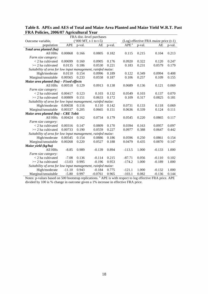
18

Table 8. APEs and AES of Total and Maize Area Planted and Maize Yield W.R.T. Past FRA Policies, 2006/07 Agricultural Year

Outcome variable, population

FRA dist.-level purchases (‘000 MT, t-1 to t-5) (Log) effective FRA maize price (t-1)

APE p-val. AE p-val. APE a p-val. AE p-val. Total area planted (ha)

All HHs 0.00868 0.166 0.0805 0.182 0.115 0.215 0.104 0.213 Farm size category:



Marginal/unsuitable 0.00565 0.233 0.0558 0.187 0.106 0.257 0.109 0.155 Maize area planted (ha) – Fixed effects




Marginal/unsuitable 0.00337 0.205 0.0665 0.151 0.0636 0.339 0.124 0.111 Maize area planted (ha) – CRE Tobit




Marginal/unsuitable 0.00268 0.220 0.0527 0.188 0.0479 0.435 0.0870 0.147 Maize yield (kg/ha)

All HHs -8.85 0.989 -0.139 0.894 -113.5 1.000 -0.133 1.000 Farm size category:

< 2 ha cultivated -7.08 0.136 -0.114 0.215 -87.71 0.056 -0.110 0.102 >= 2 ha cultivated -13.03 0.995 -0.196 0.953 -174.2 1.000 -0.189 1.000

Suitability of area for low input management, rainfed maize: High/moderate -11.10 0.943 -0.184 0.775 -121.1 1.000 -0.132 1.000

Marginal/unsuitable -5.80 0.997 -0.0761 0.965 -103.1 0.082 -0.136 0.144 Notes: p-values based on 500 bootstrap replications. a APE is with respect to log effective FRA price. APE divided by 100 is % change in outcome given a 1% increase in effective FRA price.

19

6. CONCLUSIONS AND POLICY IMPLICATIONS

Over the last decade, there has been a resurgence in direct government participation in agricultural input and output marketing in ESA. After being scaled back or eliminated during the market reforms of the 1980s and 1990s, fertilizer subsidies, parastatal GMBs, and strategic grain reserves (SGRs) are once again en vogue in the region (Jayne and Jones 1997; Jayne et al. 2002; Jayne, Chapoto, and Govereh 2007). Private grain trade remains legal in most cases, thus an increasingly important feature of grain markets in ESA is dual marketing channels: government and private sector. However, little is known about how the re-emergence of GMBs/SGRs is affecting input use and crop production by smallholder farmers in the region. In Zambia, the FRA, a SGR/GMB, has become a major player in the domestic maize market in recent years. The FRA buys maize from smallholders at a pan-territorial price that typically exceeds market prices. In this paper, we use nationally-representative panel survey data covering more than 5,000 Zambian smallholder households in the 1999/2000, 2002/2003, and 2006/2007 agricultural years to estimate the marginal effects of FRA district-level maize purchases and the effective FRA maize price on household fertilizer use on maize, and total, maize, and non-maize area planted, crop output per hectare, and crop output. The empirical models are estimated in two stages. In the first stage, we estimate the marginal effects of past FRA maize purchase and pricing policies on the mean and variance of (log) effective maize market and FRA prices at the next harvest and on the probability that a household will sell to the Agency at the next harvest. Predicted values from the first stage regressions are used to construct an expected maize price for each household and agricultural year in the panel survey. The expected maize price is then included as an explanatory variable in the second stage fertilizer demand and output supply regressions.

The empirical results point to three key findings. The empirical results point to three key findings. First, increases in past FRA maize purchases and effective prices are associated with a higher expected maize price at the next harvest. A 1% increase in past FRA district-level purchases increases households’ expected maize price in 2006/07 by 0.10%. The magnitude of this elasticity is larger for households that cultivate two or more hectares of land or are located in areas that are well suited for low input rainfed maize production. The elasticity of the expected maize price with respect to the lagged effective FRA price is also positive and statistically significant for these households. Second, the fertilizer demand and output supply regression results suggest that an increase in the expected maize price has a positive effect on total and maize area planted, a negative effect on maize yields, and no statistically significant effect on the intensity of fertilizer use on maize (kg/ha), non-maize area planted, total and non-maize output per hectare, and total, maize, and non-maize output. The marginal effects of the expected maize price on maize area planted and maize yield offset each other, the result being no significant change in maize quantity harvested. The additional area brought under maize production in response to an increase in the expected maize price may be of poorer quality and/or ill-suited for maize production, hence the decline in maize yields even with the same intensity of fertilizer use. Third, results show that for 2006/07, increases in past FRA district-level maize purchases and in the lagged effective FRA price are associated with increases in total and maize area planted, a decrease in maize yield, and no significant change in maize quantity harvested, total crop output, or the other household-level outcome variables examined. However, FRA

20

impacts on smallholder behavior via general equilibrium effects on maize, fertilizer, or other prices are not captured in this paper. Furthermore, the FRA continued to ramp up its involvement in maize marketing after 2006/07, the most recent year of the panel. Smallholders may have become more responsive to FRA activities as the Agency became a more permanent fixture of the maize marketing landscape. Part of the FRA’s strategic mission is to ensure national food security and income (FRA n.d.). Although we do not estimate the effects of past FRA behavior on food security or incomes per se, the finding of no statistically significant impact of FRA activities on maize or total crop output does not support the conclusion of improvement in food security or incomes. A large proportion of Zambia’s public resources are devoted to the FRA. For example, in the 2010/11 marketing season, spending on the FRA amounted to approximately 2% of the nation’s GDP (IMF 2011). Between 2004 and 2011, GRZ allocated an average of 25% of its annual Poverty Reduction Programmes budget to the FRA. The failure of FRA policies to increase smallholder maize and total crop output, and the fact that it is mainly relatively well off smallholders who benefit from the high FRA purchase price, calls into question the efficacy of maize price supports as a poverty reduction tool in Zambia. Indeed, at approximately 80%, rural poverty rates remain stubbornly high and there has been no substantive reduction in rural poverty since the FRA was established in 1996 (CSO 2010). GRZ and donor funds devoted to the FRA come at a high opportunity cost. Limiting FRA involvement in the maize market to securing the national strategic food reserve, its original mandate, would free up resources that could be invested in the known drivers of pro-poor agricultural growth such as agricultural research, development and extension, rural infrastructure, and education (Fan, Gulati, and Thorat 2008; World Bank 2008).

21

APPENDICES

22

APPENDIX A: SUMMARY STATISTICS

Table A.1. Summary Statistics for Continuous Explanatory Variables Percentile Explanatory variables (A) (B) Mean Std. dev. 10th 25th 50th 75th 90th FRA maize purchases in district ('000 MT, t-1) X 1.911 4.88 0 0 0 0.33 9.89 Effective FRA maize price (ZMK/kg, t-1) X 495 219 219 249 611 700 733 Maize producer price (ZMK/kg, t-1) X 447 186 219 249 498 609 661 Regional wholesale maize prices (pre-planting):

October (ZMK/kg) X 447 277 130 146 465 657 856 September (ZMK/kg) X 426 266 140 180 401 587 793 August (ZMK/kg) X 433 259 150 173 430 668 771 July (ZMK/kg) X 422 240 156 178 390 550 742 June (ZMK/kg) X 412 187 188 238 424 521 710 May (ZMK/kg) X 365 122 218 263 379 439 530 April (ZMK/kg) X 524 182 297 361 526 694 789 March (ZMK/kg) X 697 295 352 416 750 847 1,186 February (ZMK/kg) X 760 342 364 408 877 1,033 1,161 January (ZMK/kg) X 727 294 363 446 832 956 1,157 December (ZMK/kg) X 660 251 343 422 639 883 1,006 November (ZMK/kg) X 597 264 299 347 555 849 890

Effective market price of fertilizer (ZMK/kg) X X 1,442 660 720 780 1,476 1,960 2,400 Kilometers from center of SEA to nearest (as of 2000):

District town X X 34.5 22.6 9.8 16.0 28.9 47.0 70.2 Tarred/main road X X 25.5 35.7 0.9 4.0 12.0 29.2 69.8 Feeder road X X 3.3 3.3 0.6 1.1 2.4 4.3 7.7

Age of household head in 2001 X 46.1 15.4 28.0 33.0 44.0 58.0 69.0 Age of household head (time-varying) X 48.3 15.3 30.0 36.0 46.0 60.0 70.0 Landholding size (ha, cultivated+fallow land) X Xa 2.1 2.6 0.5 0.8 1.5 2.5 4.0 Full-time equivalent # of prime-age (15-59) adults X X 2.8 1.7 1.0 2.0 2.2 3.9 5.0

23

Table A.1 (Cont’d) Percentile

Explanatory variables (A) (B) MeanStd. dev. 10th 25th 50th 75th 90th

Expected growing season rainfall (mm, moving average of past 9 years)

X X 896 184 660 757 877 1,059 1,167

Expected moisture stress (20-day periods with <40mm rain, moving average of past 9 years)

X X 1.8 1.0 0.6 0.9 1.9 2.4 3.1

Rainfall variability (moving coefficient of variation of past 9 years, %)

X 22.5 6.9 13.7 17.5 21.8 26.6 30.7

Growing season rainfall (mm) Xb 969 254 639 788 943 1,140 1,258 Moisture stress (20-day periods with <40mm rain) Xb 1.4 1.4 0 0 1.0 2.0 4.0 Groundnut price (ZMK/kg, t-1, prov. median) X 1,139 355 769 900 1,053 1,400 1,667 Mixed bean price (ZMK/kg, t-1, prov. median) X 1,112 302 889 889 992 1,333 1,572 Sweet potato price (ZMK/kg, t-1, prov. median) X 214 102 100 145 193 232 386 Cattle price (ZMK/head, provincial median) X 519,656 301,918 160,000 230,000 589,388 789,138 953,272 Value of plows and harrows ('00,000 ZMK) X 0.649 2.753 0 0 0 0 2.000 % of votes won by MMD in last pres. electionc 52.2 23.9 16.8 33.5 54.7 72.5 83.6 Pct. pt. spread between MMD and leading opposition party in last pres. electionc

41.8 23.6 11.6 21.2 41.1 61.4 74.4

Notes: Variables with X in column (A) included in auxiliary regressions for expected maize price. Variables with X in column (B) included in fertilizer demand and output supply equations. N=16,566. aExcluded from area planted equations. bIncluded in output/ha equations but not area planted equations. cCandidate instrumental variable in government-subsidized fertilizer reduced form Tobit. Sources: CSO/MACO/FSRP 2001, 2004, and 2008 Supplemental Surveys.

24

Table A.2. Summary Statistics for Binary Explanatory Variables Share of households (%) Explanatory variables (A) (B) 1999/2000 2002/2003 2006/2007 HH owns radio (=1) X 34.2 47.0 57.6 HH owns cell phone (=1) X 0 0 21.1 HH does not own but has access to cell phone (=1) X 0 0 45.7 HH owns bicycle (=1) X 41.7 46.0 55.6 HH owns motorcycle (=1) X 0.5 1.1 0.9 HH owns car, pick-up, van, truck/lorry, or tractor-trailer (=1) X 1.1 0.8 1.1 HH owns ox-cart (=1) X 5.1 7.1 8.3 HH owns a water pump (=1) X 0.7 0.7 0.8 Lower primary (grades 1-4) (=1) X X 23.0 25.6 27.0 Upper primary (grades 5-7) (=1) X X 36.2 34.0 34.5 Secondary (grades 8-12) (=1) X X 19.3 18.3 19.4 Post-secondary education (=1) X X 2.5 2.7 1.8 Female-headed with non-resident husband (=1) X X 0.6 0.9 0.4 Female-headed with no husband (=1) X X 20.8 21.8 23.6 Disease-related PA male head/spouse death in last 3-4 years (=1) X 1.2 1.8 0.1 Disease-related PA female head/spouse death in last 3-4 years (=1) X 1.0 2.1 1.3 Disease-related PA male non-head/spouse death in last 3-4 years (=1) X 3.3 2.9 4.4 Disease-related PA female non-head/spouse death in last 3-4 years (=1) X 5.0 3.6 3.7 SEA is suitable for low input management maize production (=1) X X 55.3 56.0 56.4 Agro-ecological region I (low rainfall, less than 800 mm) (=1) X X 5.6 5.1 5.4 Agro-ecological region IIa (moderate rainfall, 800-1000 mm, clay soils) (=1) X X 40.4 42.1 44.1 Agro-ecological region IIb (moderate rainfall, 800-1000 mm, sandy soils) (=1) X X 9.6 9.5 8.6 Agro-ecological region III (high rainfall, over 1000 mm) (=1) X X 44.4 43.3 41.9 MMD won the constituency in the last presidential election (=1)a 92.8 44.0 59.1 Total number of households in sample 6,922 5,358 4,286 Notes: Variables with X in column (A) included in auxiliary regressions for expected maize price. Variables with X in column (B) included in fertilizer demand and output supply equations. aCandidate instrumental variable in government-subsidized fertilizer reduced form Tobit. Sources: CSO/MACO/FSRP 2001, 2004, and 2008 Supplemental Surveys.

25

Table A.3. Summary Statistics for Dependent Variables Percentile Dependent variable Ag. year Obs. Mean Std. dev. 10th 25th 50th 75th 90th Auxiliary regressions for expected maize price Effective maize market price All 4,475 427.899 237.007 179.105 243.478 375.000 560.462 695.652 Effective FRA maize price 2002/03 48 530.021 63.958 420.000 488.000 537.500 596.000 600.000 2006/07 482 687.684 55.852 640.000 660.000 690.000 720.000 745.000 HH sold maize to FRA (=1) 2002/03 5,358 0.00761

2006/07 4,286 0.0971 Reduced form Tobit for kg of gov’t-subsidized fertilizer acquired by the HH HH acquired gov’t fertilizer (=1) All 16,566 0.099 Kg of gov’t fertilizer acquired All 16,566 29.294 143.258 0 0 0 0 0 Factor demand and output supply equations HH used fertilizer on maize (=1) All 13,095 0.322 Fertilizer use on maize (kg/ha) All 13,095 85.113 176.275 0 0 0 114.286 327.869 Total area planted (ha) All 16,566 1.520 1.514 0.375 0.650 1.125 1.990 3.000 HH planted maize (=1) All 16,566 0.792 Maize area planted (ha) All 16,566 0.746 1.085 0 0.155 0.500 1.000 1.620 HH planted non-maize crop(s) (=1) All 16,566 0.794 Non-maize area planted (ha) All 16,566 0.774 0.949 0 0.180 0.500 1.013 1.820 Total output/ha (FIQI/ha) All 16,148 20.994 18.781 5.693 9.903 16.598 26.476 39.549 Maize yield (kg/ha) All 13,092 1568.644 1208.216 402.000 744.444 1240.741 2010.000 3130.328 Non-maize output/ha (FIQI/ha) All 13,087 24.316 26.741 4.763 9.511 17.329 30.025 48.091 Total output (FIQI) All 16,148 31.044 47.925 4.319 9.265 19.404 37.019 64.550 Maize output (kg) All 13,092 1504.640 2934.940 172.500 345.000 804.000 1608.000 3162.500 Non-maize output (FIQI) All 13,087 21.328 31.929 2.001 5.176 12.794 27.232 48.023 Notes: “All” refers to all three agricultural years (1999/2000, 2002/03, and 2006/07). Obs. is the number of unweighted observations. 16,566 is the total number of observations in the SS panel dataset (6,922 for SS01; 5,358 for SS04; 4,286 for SS08). Sources: CSO/MACO/FSRP 2001, 2004, and 2008 Supplemental Surveys.

26

APPENDIX B: FULL REGRESSION RESULTS

Table B.1. Results from Log Effective Market and FRA Maize Price and Log Squared Residuals Regressions Dependent variable

(A) Log effective maize market price

--------at harvest-------- (B) Log squared

--residuals from (A)--

(C) Log effective FRA maize price

--------at harvest-------- (D) Log squared

--residuals from (C)-- Explanatory variables Coef. Sig. p-val. Coef. Sig. p-val. Coef. Sig. p-val. Coef. Sig. p-val. FRA dist. purch. (‘000MT, t-1) 6.67E-3 ** 0.024 -0.149 *** 0.007 -2.06E-3 0.373 0.0153 0.825 FRA district purchases, sqd. 4.85E-3 ** 0.033 Log effective FRA price (t-1) -0.0221 0.811 1.116 0.101 0.341 *** 0.000 -4.021 * 0.074 Log eff. FRA price×1999/2000 0.417 * 0.056 0.0469 0.989 Log maize producer price (t-1) -0.0221 0.803 -14.434 0.539 1.68E-3 0.968 -1.499 0.337 Log maize producer price, sqd. 1.0156 0.580 Log regional wholesale maize price (pre-planting): October 0.127 0.365 1.058 0.257 September 0.0354 0.809 -1.850 * 0.063 August 0.0854 0.418 -0.884 0.265 July 0.0637 0.707 -2.596 ** 0.034 June -0.236 0.187 3.127 ** 0.010 May -0.0318 0.675 -0.790 0.200 April -0.155 0.446 2.306 * 0.055 March -0.119 0.546 1.845 0.173 February 0.0270 0.930 -2.016 0.345 January 0.0419 0.904 0.886 0.726 December -0.723 *** 0.005 1.658 0.287 November 0.377 *** 0.005 -2.422 ** 0.029 Log eff. market fertilizer price -0.0163 0.754 -0.521 0.168 0.0250 0.451 -2.029 0.107 HH owns radio (=1) 0.0289 * 0.079 0.0435 0.729 0.0122 0.137 0.572 0.174 HH owns cell phone (=1) 3.78E-3 0.888 0.195 0.425 7.88E-4 0.925 -7.46E-3 0.984 HH access to cell phone (=1) 3.97E-3 0.861 0.0948 0.682 -1.20E-3 0.884 -0.542 0.139 HH owns bicycle (=1) 0.0220 0.165 -0.120 0.345 -0.0111 0.211 0.0528 0.863

27

Table B.1. (Cont’d) Dependent variable


--------at harvest-------- (B) Log squared

--residuals from (A)--


--------at harvest-------- (D) Log squared

--residuals from (C)-- Explanatory variables Coef. Sig. p-val. Coef. Sig. p-val. Coef. Sig. p-val. Coef. Sig. p-val. HH owns motorcycle (=1) 5.82E-3 0.922 0.639 0.117 0.0404 0.381 -0.855 0.466 HH owns car/truck (=1) 0.0300 0.647 0.401 0.353 0.0135 0.402 -0.753 0.143 HH owns ox-cart (=1) -3.86E-3 0.891 0.393 * 0.075 -1.38E-3 0.880 -1.15E-3 0.847 Kilometers from center of SEA to nearest (as of 2000): District town 8.00E-5 0.840 4.54E-3 * 0.060 2.56E-4 0.239 8.64E-3 0.287 Tarred/main road -5.07E-4 0.216 -4.95E-4 0.829 5.88E-5 0.535 -1.81E-3 0.634 Feeder road -5.90E-3 ** 0.036 -5.70E-3 0.633 1.07E-3 0.392 -0.0293 0.618 HH head age in 2001 -5.58E-4 0.141 -0.0275 0.106 3.21E-5 0.893 -0.0107 0.293 HH head age, sqd. 1.91E-4 0.259 Highest level of education completed by HH head (base is no formal education): Lower primary (gr1-4) (=1) 0.0371 0.197 0.221 0.364 0.0488 *** 0.009 -0.503 0.512 Upper primary (gr5-7) (=1) 0.0548 * 0.052 0.421 0.106 0.0332 0.103 -0.594 0.415 Secondary (gr8-12) (=1) 0.0350 0.362 0.385 0.180 0.0567 *** 0.007 -0.451 0.563 Post-secondary (=1) 0.102 * 0.077 0.768 0.139 0.0148 0.531 -2.240 * 0.063

Gender and residence status of HH head (non-resident if <6 months; base is resident male): Female, non-res. husb. (=1) -0.108 0.129 0.608 0.285 -0.0642 ** 0.011 0.760 0.628 Female, no husband (=1) 9.54E-04 0.973 0.240 0.409 0.0383 *** 0.007 0.354 0.630

Landholding size (ha) -2.94E-4 0.901 -0.0140 0.476 5.76E-4 0.756 0.0118 0.883 Landholding size, sqd. -1.06E-5 0.302 1.78E-5 0.837 -1.21E-5 0.731 -6.39E-4 0.691 FTE PA adults -2.94E-4 0.952 -6.35E-3 0.858 4.90E-4 0.857 -0.0661 0.529 Expected rainfall (’00 mm) 0.229 0.160 -0.0379 0.861 -1.07E-4 0.995 -0.891 0.136 Expected rainfall, sqd. -0.0145 * 0.083

28

Table B.1. (Cont’d) Dependent variable


--------at harvest--------(B) Log squared

--------residuals from (A) --------


--------at harvest--------(D) Log squared

--residuals from (C)--Explanatory variables Coef. Sig. p-val. Coef. Sig. p-val. Coef. Sig. p-val. Coef. Sig. p-val.Exp. moisture stress 0.0770 * 0.075 0.668 * 0.068 -0.0128 0.716 -1.019 0.381Rain. variability (%) -5.38E-4 0.854 -0.0349 0.153 -1.88E-3 0.180 0.0563 0.195SEA suitable for low input mgt maize (=1)

-1.69E-3 0.923 -0.159 * 0.057 9.71E-3 * 0.069 0.609 ** 0.034

Agricultural year (base is 2006/2007): 1999/2000 (=1) -3.499 *** 0.003 -3.285 0.870 2002/2003 (=1) -0.400 *** 0.002 1.138 0.180 -0.224 *** 0.000 0.699 0.468

Constant 2.069 0.661 45.193 0.693 4.205 *** 0.000 9.101 0.674District dummies Yes Yes No NoProv., AER dummies No No Yes YesTime averages (CRE) Yes Yes Yes Yes Observations 4,405 4,405 492 492 R-squared 0.694 0.079 0.608 0.130 Overall model F-stat. 82.94 *** 0.000 7.62 *** 0.000 21.34 *** 0.000 3.88 *** 0.000Unbiased prediction F 0.00 1.000 0.00 1.000 0.00 1.000 0.00 1.000Theil inequal. coef. 0.800 0.541 Notes: See Tables A.1 and A.2 in Appendix A for more complete explanatory variable descriptions. FTE PA adults = full time equivalent prime age (15-59 years old) adults. AER=agro-ecological region. ***, **, * significant at the 1%, 5%, and 10% levels. Complex survey weights and Huber-White robust variance matrix estimator used in computation of standard errors. The analytical sample for the effective maize market price regression (column A) excludes the bottom and top one percent of observations in each panel survey year. For the effective FRA price regression (column B), the bottom one percent of observations in each year are excluded.

29

Table B.2. CRE Probit Results: HH Sold Maize to FRA at Harvest =1; =0 Otherwise Explanatory variables APE Sig. p-val.FRA district-level purchases (‘000 MT, t-1) 0.00303 0.427FRA district-level purchases (‘000 MT, t-2) 0.0146 0.158FRA district-level purchases (‘000 MT, t-3) -0.00670 0.703FRA district-level purchases (‘000 MT, t-4) 0.00784 0.764FRA district-level purchases (‘000 MT, t-5) 0.0128 0.214Log effective FRA price (t-1) 0.279 *** 0.003Log maize producer price (t-1) -0.180 *** 0.005Log effective market fertilizer price -0.0721 0.168HH owns radio (=1) 0.0146 0.150HH owns cell phone (=1) 0.0173 0.164HH does not own but has access to cell phone (=1) 0.0145 0.126HH owns bicycle (=1) 0.0245 ** 0.029HH owns car/truck (=1) 0.0382 0.440HH owns ox-cart (=1) 0.0282 0.188Km from center of SEA to nearest district town (as of 2000) 0.000415 0.187Km from center of SEA to nearest tarred/main road (as of 2000) 0.000104 0.640Km from center of SEA to nearest feeder road (as of 2000) -0.00561 *** 0.002HH head age in 2001 -0.000122 0.631Highest level of education completed by HH head (base is no formal education): Lower primary (grades 1-4) (=1) -0.0187 0.274Upper primary (grades 5-7) (=1) -0.0163 0.353Secondary (grades 8-12) (=1) -0.00323 0.883Post-secondary (=1) -0.0201 0.500

Female HH head (=1) -0.0208 0.193Landholding size (ha)a 0.0107 *** 0.000Full-time equivalent prime-age adults (ages 15-59) 0.00209 0.434Expected growing season rainfall (’00 mm)b 0.00678 0.734Expected moisture stress (# of 20-day periods) -0.0260 0.502Rainfall variability (%) 0.00436 * 0.060SEA suitable for low input mgt rainfed maize production (=1) 0.00514 0.6412002/2003 agricultural year (=1) (2006/2007 is base year) -0.0384 0.170Province and agro-ecological region dummies Yes Time averages (CRE) Yes Observations 5,441 Number of observations with dependent variable =1 503 Overall model F-stat. 15.49 *** 0.000Joint significance of lagged FRA district-level purchases (F-stat.) 3.77 *** 0.003Long-run effect of FRA district-level purchases (‘000 MT) 0.0315 * 0.058Notes: ***, **, * significant at the 1%, 5%, and 10% levels. Complex survey weights and Huber-White robust variance matrix estimator used in computation of standard errors. aAPE includes effect of squared and cubed terms. bAPE includes effect of squared term.

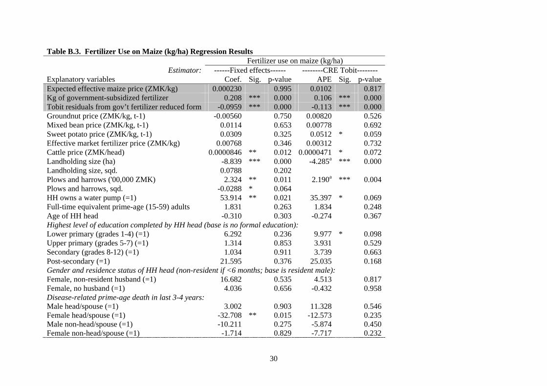
30

Table B.3. Fertilizer Use on Maize (kg/ha) Regression Results Fertilizer use on maize (kg/ha)

Estimator: ------Fixed effects------ --------CRE Tobit-------- Explanatory variables Coef. Sig. p-value APE Sig. p-valueExpected effective maize price (ZMK/kg) 0.000230 0.995 0.0102 0.817Kg of government-subsidized fertilizer 0.208 *** 0.000 0.106 *** 0.000Tobit residuals from gov’t fertilizer reduced form -0.0959 *** 0.000 -0.113 *** 0.000Groundnut price (ZMK/kg, t-1) -0.00560 0.750 0.00820 0.526Mixed bean price (ZMK/kg, t-1) 0.0114 0.653 0.00778 0.692Sweet potato price (ZMK/kg, t-1) 0.0309 0.325 0.0512 * 0.059Effective market fertilizer price (ZMK/kg) 0.00768 0.346 0.00312 0.732Cattle price (ZMK/head) 0.0000846 ** 0.012 0.0000471 * 0.072Landholding size (ha) -8.839 *** 0.000 -4.285a *** 0.000Landholding size, sqd. 0.0788 0.202 Plows and harrows ('00,000 ZMK) 2.324 ** 0.011 2.190a *** 0.004Plows and harrows, sqd. -0.0288 * 0.064 HH owns a water pump (=1) 53.914 ** 0.021 35.397 * 0.069Full-time equivalent prime-age (15-59) adults 1.831 0.263 1.834 0.248Age of HH head -0.310 0.303 -0.274 0.367Highest level of education completed by HH head (base is no formal education): Lower primary (grades 1-4) (=1) 6.292 0.236 9.977 * 0.098Upper primary (grades 5-7) (=1) 1.314 0.853 3.931 0.529Secondary (grades 8-12) (=1) 1.034 0.911 3.739 0.663Post-secondary (=1) 21.595 0.376 25.035 0.168Gender and residence status of HH head (non-resident if <6 months; base is resident male): Female, non-resident husband (=1) 16.682 0.535 4.513 0.817Female, no husband (=1) 4.036 0.656 -0.432 0.958Disease-related prime-age death in last 3-4 years: Male head/spouse (=1) 3.002 0.903 11.328 0.546Female head/spouse (=1) -32.708 ** 0.015 -12.573 0.235Male non-head/spouse (=1) -10.211 0.275 -5.874 0.450Female non-head/spouse (=1) -1.714 0.829 -7.717 0.232

31

Table B.3. (Cont’d) Fertilizer use on maize (kg/ha)

Estimator: ------Fixed effects------ --------CRE Tobit--------Explanatory variables Coef. Sig. p-value APE Sig. p-valueKm from center of SEA to nearest (as of 2000): District town -0.577 *** 0.000Tarred/main road 0.0979 0.263Feeder road -0.921 0.467 Expected rainfall (’00 mm) -0.858 0.881 -2.506 0.659Expected moisture stress (#20-day periods) -15.520 ** 0.044 -4.894 0.585SEA suitable for low input management maize (=1) 0.696 0.908Agricultural year (base is 2006/2007): 1999/2000 (=1) 85.532 *** 0.004 71.691 * 0.0562002/2003 (=1) 40.287 *** 0.003 32.684 * 0.022 Constant 100.052 0.196Province and agro-region dummies N/A YesTime averages (CRE) N/A Yes Observations 11,953 11,953Within R-squared (pseudo R-squared for Tobit) 0.087 0.054Overall model F-stat. 9.30 *** 0.000 26.56 *** 0.000Hansen J test for over-identifying restrictions 2.086 0.352Notes: ***, **, * significant at the 1%, 5%, and 10% levels. p-values from standard errors based on 500 bootstrap replications to account for generated regressor (Tobit residuals from government fertilizer reduced form). aAPE includes effect of squared term.

32

Table B.4. Total and Maize Area Planted (ha) Regression Results Total area planted (ha) Maize area planted (ha)

Estimator: ------Fixed effects------ ------Fixed effects------ --------CRE Tobit-------- Explanatory variables Coef. Sig. p-val. Coef. Sig. p-val. APE Sig. p-val. Expected effective maize price (ZMK/kg) 0.00148 * 0.063 8.81E-4 ** 0.044 6.26E-4 * 0.063 Kg of government-subsidized fertilizer 0.00147 *** 0.000 0.00122 *** 0.000 8.52E-4 *** 0.000 Tobit residuals from gov’t fertilizer reduced form Excluded 0.559 Excluded 0.197 Excluded 0.150 Groundnut price (ZMK/kg, t-1) -6.99E-4 *** 0.000 -4.41E-4 *** 0.000 -2.86E-4 *** 0.000 Mixed bean price (ZMK/kg, t-1) -1.16E-4 0.554 5.10E-5 0.696 3.43E-6 0.975 Sweet potato price (ZMK/kg, t-1) 2.83E-4 0.271 -2.88E-4 ** 0.035 -2.59E-4 ** 0.022 Effective market fertilizer price (ZMK/kg) 1.76E-4 ** 0.026 3.64E-5 0.490 1.82E-5 0.650 Cattle price (ZMK/head) 0.000 0.885 0.000 0.422 0.000 0.403 Plows and harrows ('00,000 ZMK) 0.101 *** 0.000 0.0700 *** 0.000 0.0455a *** 0.000 Plows and harrows, sqd. -5.89E-4 * 0.071 -3.21E-4 0.277 HH owns a water pump (=1) 0.452 0.202 0.0513 0.795 0.0300 0.825 Full-time equivalent prime-age (15-59) adults 0.0601 ** 0.034 0.0361 * 0.076 0.0370a *** 0.000 Full-time equivalent prime-age adults, sqd. 0.00301 0.399 0.00120 0.641 Age of HH head 0.0555 *** 0.000 0.0275 *** 0.000 0.00545a *** 0.000 Age of HH head, sqd. -4.70E-4 *** 0.000 -2.29E-4 *** 0.000 Highest level of education completed by HH head (base is no formal education): Lower primary (grades 1-4) (=1) 0.0366 0.385 -0.00447 0.852 -0.00122 0.951 Upper primary (grades 5-7) (=1) 0.0439 0.417 -0.00357 0.907 0.0105 0.674 Secondary (grades 8-12) (=1) 0.115 * 0.100 0.0210 0.623 0.0250 0.467 Post-secondary (=1) 0.138 0.342 -0.0462 0.646 -0.0212 0.785 Gender and residence status of HH head (non-resident if <6 months; base is resident male): Female, non-resident husband (=1) 0.144 0.223 0.148 ** 0.037 0.178 *** 0.009 Female, no husband (=1) -0.306 *** 0.000 -0.160 *** 0.000 -0.129 *** 0.000

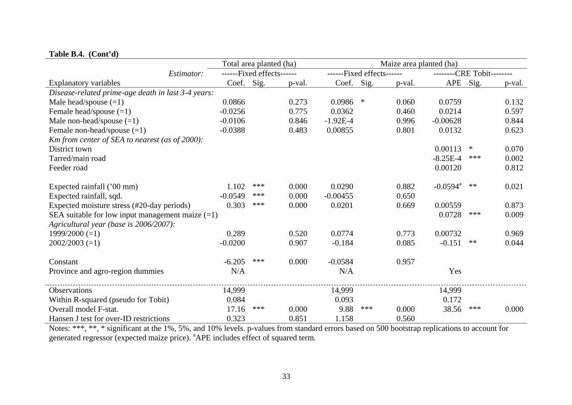
33

Table B.4. (Cont’d) Total area planted (ha) Maize area planted (ha)

Estimator: ------Fixed effects------ ------Fixed effects------ --------CRE Tobit-------- Explanatory variables Coef. Sig. p-val. Coef. Sig. p-val. APE Sig. p-val. Disease-related prime-age death in last 3-4 years: Male head/spouse (=1) 0.0866 0.273 0.0986 * 0.060 0.0759 0.132 Female head/spouse (=1) -0.0256 0.775 0.0362 0.460 0.0214 0.597 Male non-head/spouse (=1) -0.0106 0.846 -1.92E-4 0.996 -0.00628 0.844 Female non-head/spouse (=1) -0.0388 0.483 0.00855 0.801 0.0132 0.623 Km from center of SEA to nearest (as of 2000): District town 0.00113 * 0.070 Tarred/main road -8.25E-4 *** 0.002 Feeder road 0.00120 0.812 Expected rainfall (’00 mm) 1.102 *** 0.000 0.0290 0.882 -0.0594a ** 0.021 Expected rainfall, sqd. -0.0549 *** 0.000 -0.00455 0.650 Expected moisture stress (#20-day periods) 0.303 *** 0.000 0.0201 0.669 0.00559 0.873 SEA suitable for low input management maize (=1) 0.0728 *** 0.009 Agricultural year (base is 2006/2007): 1999/2000 (=1) 0.289 0.520 0.0774 0.773 0.00732 0.969 2002/2003 (=1) -0.0200 0.907 -0.184 0.085 -0.151 ** 0.044 Constant -6.205 *** 0.000 -0.0584 0.957 Province and agro-region dummies N/A N/A Yes Observations 14,999 14,999 14,999 Within R-squared (pseudo for Tobit) 0.084 0.093 0.172 Overall model F-stat. 17.16 *** 0.000 9.88 *** 0.000 38.56 *** 0.000 Hansen J test for over-ID restrictions 0.323 0.851 1.158 0.560 Notes: ***, **, * significant at the 1%, 5%, and 10% levels. p-values from standard errors based on 500 bootstrap replications to account for generated regressor (expected maize price). aAPE includes effect of squared term.

34

Table B.5. Total, Maize, and Non-maize Output per Hectare Regression Results Total (FIQI/ha) Maize (kg/ha) Non-maize (FIQI/ha)

Estimator: ------Fixed effects------ ------Fixed effects------ ------Fixed effects------ Explanatory variables Coef. Sig. p-val. Coef. Sig. p-val. Coef. Sig. p-val. Expected effective maize price (ZMK/kg) -8.42E-4 0.897 -1.388 *** 0.007 0.0114 0.327 Kg of government-subsidized fertilizer 0.00912 *** 0.000 0.739 *** 0.000 0.00705 ** 0.043 Tobit residuals from gov’t fertilizer reduced form -0.00877 *** 0.001 -0.421 ** 0.045 -0.0142 ** 0.014 Groundnut price (ZMK/kg, t-1) 5.90E-4 0.778 0.795 *** 0.000 -0.00405 0.401 Mixed bean price (ZMK/kg, t-1) 0.0132 *** 0.000 -0.285 0.310 0.0296 *** 0.000 Sweet potato price (ZMK/kg, t-1) 0.00210 0.611 -0.467 * 0.098 0.00873 0.245 Effective market fertilizer price (ZMK/kg) -0.00100 0.329 -0.109 0.160 -0.00286 0.195 Cattle price (ZMK/head) -3.70E-6 0.364 9.32E-4 *** 0.004 -1.94E-5 *** 0.005 Landholding size (ha) -1.815 *** 0.000 -89.219 *** 0.000 -2.380 *** 0.000 Landholding size, sqd. 0.0247 0.105 1.249 0.160 0.0286 * 0.081 Plows and harrows ('00,000 ZMK) 0.311 ** 0.020 10.506 * 0.068 0.364 ** 0.035 Plows and harrows, sqd. -0.00221 0.340 HH owns a water pump (=1) 2.120 0.325 267.771 0.161 -0.187 0.955 Full-time equivalent prime-age (15-59) adults -0.291 0.461 -22.516 0.437 0.435 0.176 Full-time equivalent prime-age adults, sqd. 0.0634 0.182 5.291 0.119 Age of HH head 0.305 * 0.065 -0.386 0.902 -0.120 0.171 Age of HH head, sqd. -0.00361 ** 0.021 Highest level of education completed by HH head (base is no formal education): Lower primary (grades 1-4) (=1) 0.382 0.621 78.831 0.165 0.451 0.510 Upper primary (grades 5-7) (=1) -0.839 0.355 62.985 0.350 0.106 0.193 Secondary (grades 8-12) (=1) -0.377 0.732 48.125 0.586 0.359 0.436 Post-secondary (=1) 0.524 0.796 141.007 0.371 0.747 0.749 Gender and residence status of HH head (non-resident if <6 months; base is resident male): Female, non-resident husband (=1) 0.356 0.879 -204.135 0.187 0.776 0.802 Female, no husband (=1) -0.629 0.502 -33.844 0.660 0.464 0.446

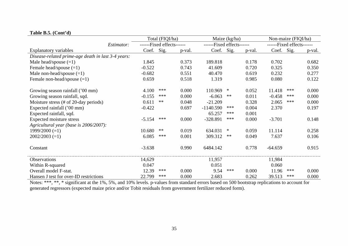
35

Table B.5. (Cont’d) Total (FIQI/ha) Maize (kg/ha) Non-maize (FIQI/ha)

Estimator: ------Fixed effects------ ------Fixed effects------ ------Fixed effects------ Explanatory variables Coef. Sig. p-val. Coef. Sig. p-val. Coef. Sig. p-val. Disease-related prime-age death in last 3-4 years: Male head/spouse (=1) 1.845 0.373 189.818 0.178 0.702 0.682 Female head/spouse (=1) -0.522 0.743 41.609 0.720 0.325 0.350 Male non-head/spouse (=1) -0.682 0.551 40.470 0.619 0.232 0.277 Female non-head/spouse (=1) 0.659 0.518 1.319 0.985 0.080 0.122 Growing season rainfall (’00 mm) 4.100 *** 0.000 110.969 * 0.052 11.418 *** 0.000 Growing season rainfall, sqd. -0.155 *** 0.000 -6.063 ** 0.011 -0.458 *** 0.000 Moisture stress (# of 20-day periods) 0.611 ** 0.048 -21.209 0.328 2.065 *** 0.000 Expected rainfall (’00 mm) -0.422 0.697 -1140.590 *** 0.004 2.370 0.197 Expected rainfall, sqd. 65.257 *** 0.001 Expected moisture stress -5.154 *** 0.000 -328.891 *** 0.000 -3.701 0.148 Agricultural year (base is 2006/2007): 1999/2000 (=1) 10.680 ** 0.019 634.031 * 0.059 11.114 0.258 2002/2003 (=1) 6.085 *** 0.001 309.312 ** 0.049 7.637 0.106 Constant -3.638 0.990 6484.142 0.778 -64.659 0.915 Observations 14,629 11,957 11,984 Within R-squared 0.047 0.051 0.060 Overall model F-stat. 12.39 *** 0.000 9.54 *** 0.000 11.96 *** 0.000 Hansen J test for over-ID restrictions 22.799 *** 0.000 2.683 0.262 39.513 *** 0.000 Notes: ***, **, * significant at the 1%, 5%, and 10% levels. p-values from standard errors based on 500 bootstrap replications to account for generated regressors (expected maize price and/or Tobit residuals from government fertilizer reduced form).

36

REFERENCES

Barrett, Christopher B. and Emelly Mutambatsere. 2008. Marketing Boards. In The New Palgrave Dictionary of Economics, Second Edition, ed. Steven N. Durlauf and Lawrence E. Blume. London: Palgrave Macmillan.

Central Statistical Office (CSO). 2010. Poverty Trends Report, 1996-2006. Lusaka: CSO.

Denning, Glenn, Patrick Kabambe, Pedro Sanchez, Alia Malik, Rafael Flor, Rebbie Harawa, Phelire Nkhoma, Colleen Zamba, Clement Banda, Chrispin Magombo, Michael Keating, Justine Wangila, and Jeffrey Sachs. 2009. Inputs Subsidies to Improve Smallholder Maize Productivity in Malawi: Toward an African Green Revolution. PLoSBiology 7.1: e1000023.

Diewert, W. Erwin 1992. Fisher Ideal Output, Input, and Productivity Indexes Revisited. The Journal of Productivity Analysis 3.3: 211-48.

Diewert, W. Erwin 1993. Index Numbers. In Essays in Index Number Theory, ed. W. Erwin

Diewert and Alice O. Nakamura. New York: North-Holland. Duflo, Esther, Michael Kremer, and Jonathan Robinson. 2009. Nudging Farmers to Use

Fertilizer: Theory and Experimental Evidence from Kenya. National Bureau of Economic Research (NBER) Working Paper No. 15131. Cambridge, MA: NBER.

Dugger, Celia W. 2007. Ending Famine, Simply by Ignoring the Experts. New York Times, 7

December. Fan, Shenggen, Ashok Gulati, and Sudhadeo Thorat. 2008. Investment, Subsidies, and Pro-

poor Growth in Rural India. Agricultural Economics 39: 163-70. FEWSNET (Famine Early Warning Systems Network). 2003a. Zambia: Monthly Report,

May 2003. http://www.fews.net/Pages/countryarchive.aspx?pid=500&gb=zm&l=en FEWSNET. 2003b. Zambia: Monthly Report, June 2003 – Food Security Position Improves.

http://www.fews.net/Pages/countryarchive.aspx?pid=500&gb=zm&l=en FEWSNET and WFP (World Food Programme). 2002. Zambia: Special July 2002 Monthly

Report. http://www.fews.net/Pages/countryarchive.aspx?pid=500&gb=zm&l=en Food Reserve Agency (FRA). n.d. FRA website. Accessed November 5, 2010.

http://www.fra.org.zm/ FRA. Various years. Crop Marketing Arrangements for 20XX/YY Marketing Seasons.

Lusaka: FRA. Government of the Republic of Zambia (GRZ). 1995. Food Reserve Act, 1995.

http://www.fao.org/docrep/w4979e/w4979e0l.htm GRZ. 2005. Act No. 20 of 2005: An Act to Amend the Food Reserve Act. http://www.parliament.gov.zm/index.php?option=com_docman&task=doc_download &gid=543

http://www.fews.net/Pages/countryarchive.aspx?pid=500&gb=zm&l=en



http://www.fra.org.zm/

http://www.fao.org/docrep/w4979e/w4979e0l.htm

http://www.parliament.gov.zm/index.php?option=com_docman&task=doc_download

37

International Monetary Fund (IMF). 2011. Zambia: Sixth Review under the Three-year Arrangement under the Extended Credit Facility, Requests for Waiver of Nonobservance of Performance Criterion, and Financing Assurances Review. IMF Country Report No. 11/196, July. Washington, D.C.: IMF.

Jansen, Doris. 1991. Zambia. In The Political Economy of Agricultural Pricing Policy,

Volume 3: Africa and the Mediterranean, ed. Anne O. Krueger, Maurice Schiff, and Alberto Valdés. Baltimore: The Johns Hopkins University Press.

Jayne, T.S., Antony Chapoto, and Jones Govereh. 2007. Grain Marketing Policy at the

Crossroads: Challenges for Eastern and Southern Africa. Paper presented at the FAO Workshop on Staple Food Trade and Market Policy Options for Promoting Developing in Eastern and Southern Africa, 1-2 March. Rome, Italy.

Jayne, T.S., Jones Govereh, Anthony Mwanaumo, James K. Nyoro, and Antony Chapoto.

2002. False Promise or False Premise? The Experience of Food and Input Market Reform in Eastern and Southern Africa. World Development 30.11: 1967-85.

Jayne, T.S. and Stephen Jones. 1997. Food Marketing and Price Policy in Eastern and

Southern Africa: A Survey. World Development 25.9: 1505-27. Jayne, T. S., Robert J. Myers, and James K. Nyoro. 2008. The Effects of NCPB Marketing

Policies on Maize Market Prices in Kenya. Agricultural Economics 38: 313-25. Kapekele, Mutale. 2010. Ngwenya Ties Malawi’s Success in Agriculture to Government

Subsidies. The Post (Zambia). 22 May 22. http://www.postzambia.com/post-read_article.php?articleId=9480 Krueger, Anne O. 1991. The Political Economy of Agricultural Pricing Policy, Volume 5: A

Synthesis of the Political Economy in Developing Countries. Baltimore: The Johns Hopkins University Press.

Krueger, Anne O. 1996. Political Economy of Agricultural Policy. Public Choice 87.1/2:

163-75. Lien, Donald. 2005. On the Minimum and Maximum of Bivariate Lognormal Random

Variables. Extremes 8.1-2: 79-83. Mason, Nicole M. 2011. Marketing Boards, Fertilizer Subsidies, Prices, and Smallholder

Behavior: Modeling and Policy Implications for Zambia. Ph.D. dissertation, Michigan State University.

Mason, Nicole M. and Robert J. Myers. 2011. The Effects of the Food Reserve Agency on

Maize Market Prices in Zambia: Are there Threshold Nonlinearities? Unpublished manuscript.

Masters, William A. and Ernst-August Nuppenau. 1993. Panterritorial versus Regional

Pricing for Maize in Zimbabwe. World Development 21.10: 1647-58.

http://www.postzambia.com/post-read_article.php?articleId=9480

38

Megill, David J. 2005. Recommendations for Adjusting Weights for Zambia Post-Harvest Survey Data Series and Improving Estimation Methodology for Future Surveys. FSRP Working Paper No. 13. Lusaka: Food Security Research Project. http://www.aec.msu.edu/fs2/zambia/wp13_zambia.pdf

Minot, Nicholas. 2010. Food Price Stabilization: Lessons from Eastern and Southern Africa.

Paper prepared for the Fourth African Agricultural Markets Program (AAMP) policy symposium, Agricultural Risks Management in Africa: Taking Stock of what Has and Hasn’t Worked, 6-10 September. Lilongwe, Malawi.

Ricker-Gilbert, Jacob, T.S. Jayne, and Ephraim Chirwa. 2011. Subsidies and Crowding out:

A Double-hurdle Model of Fertilizer Demand in Malawi. American Journal of Agricultural Economics 93.1: 26-42.

Schiff, Maurice and Alberto Valdés. 1991. The Political Economy of Agricultural Pricing

Policy, Volume 4: A Synthesis of the Economics in Developing Countries. Baltimore: The Johns Hopkins University Press.

Staatz, John. 2006. Marketing Orders and Marketing Boards. Handout for Agricultural

Economics 841: Analysis of Food System Organizations and Performance. East Lansing: Michigan State University.

Wooldridge, Jeffrey M. 2002. Econometric Analysis of Cross Section and Panel Data.

Cambridge, Massachusetts: MIT Press. World Bank. 2008. World Development Report 2008: Agriculture for Development.

Washington D.C.: The World Bank.

http://www.aec.msu.edu/fs2/zambia/wp13_zambia.pdf

zambian smallholder behavioral responses to food reserve agency activities

Documents