Supplementary material for the paper:

Naming Game on Networks:Let Everyone be Both Speaker and Hearer

Yuan Gao, Guanrong Chen and Rosa H. M. Chan

July 25, 2014

The small-world network by WS model with different initial connected neighbour K are in-vestigated, the configuration properties are illustrated in Table S1.

Network #Nodes < D > < PL > < CC >

SW with K = 20 and RP = 0.2 (WS − 20− 0.2) 1000 40.0 2.4651 0.3837SW with K = 30 and RP = 0.2 (WS − 30− 0.2) 1000 60.0 2.1621 0.3937SW with K = 50 and RP = 0.2 (WS − 50− 0.2) 1000 100.0 1.9140 0.4055

Table S1: Small-world Networks with differnt initial connected neighbour K. Where RP is therewiring probability, < D > is average degree, < PL > is average path length and < CC > isaverage clustering coefficient.

The Success Ratio and the three metrics for various β on WS networks with different < D >and same N = 20 are shown in Figure S1 and Figure S2, respecitively. From them, it can beobserved that (i) bothNtotal max andNdiff max increases with< D >, because the Success Ratioof mid-iteration is relatively smaller for networks with larger < D >. (ii) Niter cvg decreases with< D > increasing, the reason is when < D > is small, each node in WS networks only connectwith only a few number of its “nearest neighbour”, i.e., the whole network are more “locallyconnected” and the intra-group consensus words are hard to be spread to far away, thus finallyleads to a longer convergence time.

Figure S1: Success Ratio for each iteration with β equal to 0.1, 0.5, and 1 on WS networks withvarious< D >. The group sizeN for all simulations are 20. The network configurations (in orderof RED, BLACK, GLUE) are WS − 20− 0.2,WS − 30− 0.2,WS − 50− 0.2. Columns fromleft to right are the Success Ratio for β =0.1, 0.5 and 1, respectively.

The comparison of NGG and NGMH with different group size N equal to 10, 50, 100 can befound in Figure S3 - S5, respectively. The analysis of these results is consensus with that in themain text.

1

Figure S2: The three convergence metrics for group size N = 20 on WS networks with various< D >. The network configurations (in order of RED, BLACK, GLUE) areWS−20−0.2,WS−30 − 0.2,WS − 50 − 0.2. Columns from left to right indicates the illustrations for Ntotal max,Ndiff max and Niter cvg (log-scale in Y-axis), respectively.

Figure S3: The convergence of the NGG model for group size N equal to 10. Both Number ofDifferent Words vs. #Iteration and Number of Total Words vs. #Iteration are investigated. Threedifferent β as well as NGMH are compared. The tested network configurations are RG − 0.05,WS − 20− 0.2 and BA− 50.

Figure S4: The convergence of the NGG model for group size N equal to 50. Other parametersare same as Figure S3.

2

Figure S5: The convergence of the NGG model for group size N equal to 100. Other parametersare same as Figure S3.

The Success Ratio for various β from 0.1 to 0.9 on the network configurations of Table 1are illustrated in Figure S6 - S8, for RG, WS, BA model respectively. The Success Ratio for allnetworks types increase monotonously with β

Figure S6: The Success Ratio for various β from 0.1 to 0.9 on the RG networks with various groupsize N . The tested samples are RG− 0.03 with N = 20, RG− 0.05 with N = {10, 20, 50, 100},RG− 0.1 with N = 20.

3

Figure S7: The Success Ratio for various β from 0.1 to 0.9 on the WS networks with variousgroup size N . The tested samples are WS − 20 − 0.1 with N = 20, WS − 20 − 0.2 withN = {10, 20, 50, 100}, WS − 20− 0.3 with N = 20.

Figure S8: The Success Ratio for various β from 0.1 to 0.9 on the WS networks with various groupsize N . The tested samples are BA − 25 with N = 20, BA − 50 with N = {10, 20, 50, 100},BA− 75 with N = 20.

4

For the comparison of three metricsM (i.e.,Ntotal max, Ndiff max, Niter cvg) between NGMHand our method, the results of NGMH for the network configurations used in main text are listedin Table S2. All observations of Subsection Convergence of NGG hold when compare Table S2with Figure 4 - 6.

Network Configurations Ntotal max Ndiff max Niter cvg

RG− 0.03, N = 20 3446.35 50.90 2177.65 (≈ 103.34)RG− 0.05, N = 10 4944.00 101.95 4809.15 (≈ 103.68)RG− 0.05, N = 20 3722.50 49.95 2080.85 (≈ 103.32)RG− 0.05, N = 50 2706.75 21.80 633.95 (≈ 102.80)RG− 0.05, N = 100 2629.55 20.15 619.05 (≈ 102.79)RG− 0.1, N = 20 3793.75 49.55 1843.25 (≈ 103.27)SW − 20− 0.1, N = 20 1763.35 49.10 8107.75 (≈ 103.91)SW − 20− 0.2, N = 10 2799.70 100.50 8522.20 (≈ 103.93)SW − 20− 0.2, N = 20 2214.35 49.95 4612.85 (≈ 103.66)SW − 20− 0.2, N = 50 1789.65 23.85 1889.50 (≈ 103.28)SW − 20− 0.2, N = 100 1832.45 25.15 1768.20 (≈ 103.25)SW − 20− 0.3, N = 20 2629.85 51.35 3022.90 (≈ 103.48)BA− 25, N = 20 3584.30 63.35 2517.50 (≈ 103.40)BA− 50, N = 10 5069.85 119.70 6002.25 (≈ 103.78)BA− 50, N = 20 3770.70 60.85 2463.50 (≈ 103.39)BA− 50, N = 50 2904.60 26.20 771.20 (≈ 102.89)BA− 50, N = 100 2235.55 17.15 410.55 (≈ 102.61)BA− 75, N = 20 3879.00 59.20 2452.30 (≈ 103.39)

Table S2: The three metrics, Ntotal max, Ndiff max andNiter cvg on the selected network configu-rations. The selected network configurations are same as these used in Figure 4 - 6, i.e.,RG−0.03with N = 20, RG− 0.05 with N = {10, 20, 50, 100}, RG− 0.1 with N = 20 for RG networks;WS − 20− 0.1 with N = 20, WS − 20− 0.2 with N = {10, 20, 50, 100}, WS − 20− 0.3 withN = 20 for WS networks; and BA − 25 with N = 20, BA − 50 with N = {10, 20, 50, 100},BA− 75 with N = 20 for BA networks.

Figure S9: The numerical evidence for the analysis of the alteration of Ntotal max and Ndiff max

on RG networks. RG − 0.05 with N = 10, 20, 50 are chosen for illustration since the differenceof SR among them are significant. β from 0.1 - 0.3 are used, because it is not too large to lead thesaturation of SR in the initial iterations. Rows from top to bottom: the Ntotal max, the SR and theNdiff max of each iterations. Column from left to right: β = 0.1, 0.2, 0.3.

5

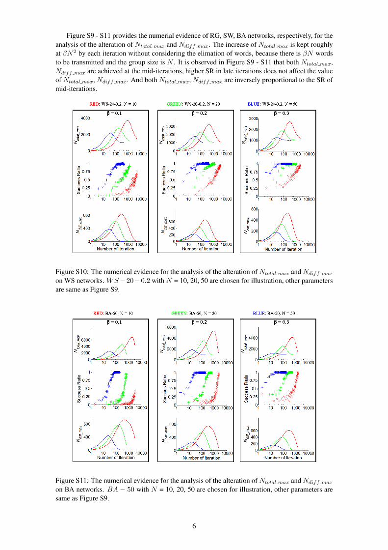
Figure S9 - S11 provides the numerial evidence of RG, SW, BA networks, respectively, for theanalysis of the alteration of Ntotal max and Ndiff max. The increase of Ntotal max is kept roughlyat βN2 by each iteration without considering the elimation of words, because there is βN wordsto be transmitted and the group size is N . It is observed in Figure S9 - S11 that both Ntotal max,Ndiff max are achieved at the mid-iterations, higher SR in late iterations does not affect the valueof Ntotal max, Ndiff max. And both Ntotal max, Ndiff max are inversely proportional to the SR ofmid-iterations.

Figure S10: The numerical evidence for the analysis of the alteration of Ntotal max and Ndiff max

on WS networks. WS−20−0.2 with N = 10, 20, 50 are chosen for illustration, other parametersare same as Figure S9.

Figure S11: The numerical evidence for the analysis of the alteration of Ntotal max and Ndiff max

on BA networks. BA − 50 with N = 10, 20, 50 are chosen for illustration, other parameters aresame as Figure S9.

6