1

Richardson-Lucy Deblurring for Scenes underProjective Motion Path

Yu-Wing Tai Ping Tan Long Gao Michael S. Brown

Abstract— This paper addresses the problem of modeling andcorrecting image blur caused by camera motion that follows aprojective motion path. We introduce a new Projective MotionBlur Model that treats the blurred image as an integration ofa clear scene under a sequence of projective transformationsthat describe the camera’s path. The benefits of this motion blurmodel is that it compactly represents spatially varying motionblur without the need for explicit blurs kernels or having tosegment the image into local regions with the same spatiallyinvariant blur. We show how to modify the Richardson-Lucy(RL) algorithm to incorporate our Projective Motion Blur Modelto estimate the original clear image. In addition, we will showthat our Projective Motion RL algorithm can incorporate state-of-the-art regularization priors to improve the deblurred results.Our Projective Motion Blur Model along with the ProjectiveMotion RL is detailed together with statistical analysis on thealgorithm’s convergence properties, robustness to noise, andexperimental results demonstrating its overall effectiveness fordeblurring images.

I. I NTRODUCTION

Motion blur is an artifact in photography caused by the relativemotion between the camera and an imaged scene during exposure.Ignoring the effects of defocusing and lens abbreviation, eachpoint in the blurred image can be considered the result ofconvolution by a point spread function (PSF), i.e. a motionblur kernel, that describes the relative motion trajectory at thatpixel position. The aim of image deblurring is to reverse thisconvolution process in order to recover a clear image of the scenefrom the captured blurry image.

A common assumption in motion deblurring is that the motionPSF describing the motion blur is spatially invariant. This impliesthat the motion blur effect is caused by camera ego motionthat can be described by a global PSF. Artifacts arising frommoving objects and depth variations in the scene are ignored.As recently discussed by Levinet al. [18], this global PSFassumption for blurred images caused by camera motion is invalidfor practical purposes. In their experiments, images taken withcameras undergoing hand shake exhibited notable amounts ofcamera rotation that causes spatially varying motion blur withinthe image. As a result, Levinet al. [18] advocated the need forbetter motion blur models as well as image priors to impose onthe deblurred results. In this paper, we address the former issueby introducing a new and compact motion blur model that is ableto describe spatially varying motion blur caused by a cameraundergoing a projective motion path. An example of the typeof blur caused by a projective motion path and that of resultsobtained from our algorithm are shown in Figure 1.

We refer to our model as theProjective Motion Blur Model,as it represents the degraded image as an integration of the clearscene under a sequence of projective motions (Figure 2). The

(a)RMS: 47.2736 (b)RMS: 10.5106

(c)RMS: 10.3517 (d) Ground truth

Fig. 1. (a) An image degraded by spatially varying motion blur. (b) Ourresult from our basic algorithm. (c) Our result with added regularization. (d)Ground truth image. TheRMS errors are also shown below each image.

benefits of our model is that we do not explicitly require a PSF todescribe the blur at any point in the image, thus our approach canbe considered “kernel free”. Likewise, we do not need to segmentthe image into regions of locally similar spatially invariant blur,as done in several previous approaches [15], [2], [7]. This makesour our approach compact in terms of its ability to describe theunderlying motion blur without the need for local blur kernels.However, because our approach is not based on convolution withan explicit PSF, it has no apparent frequency domain equivalent.Therefore, one of the key contribution of this paper is to showhow our blur model can be used to extend the conventional pixel-domain Richardson-Lucy (RL) deblurring algorithm to correctspatially varying motion blur.

We refer to this modified RL algorithm as theProjectiveMotion Richardson-Lucy algorithm. Similar to the conventionalRL algorithm, regularization derived from image priors can beincorporated into our algorithm. We note that in this paper,

= dt∫ ...

...

Blur image

Fig. 2. Our input image is considered the integration of an image sceneunder projective motion .

our work is focused on developing the projective motion blurmodel and the associated RL algorithm. We will assume in ourexamples that the motion path of the camera is known and thatthe camera’s motion satisfies our Projective Motion Blur Model.Potential methods for accurately estimating the projective motionpath are discussed briefly in Section VI. As with other deblurringapproaches, we assume that the scene is distance and does notcontain moving objects.

The remainder of this paper is organized as follows: Section IIdiscusses related work; Section III details our motion blur model;Section IV derives the Projective Motion Richardson-Lucy de-convolution algorithm; Section V describes how to incorporateregularization into our Projective Motion RL deconvolution algo-rithm with additional implementation details; Section VI discussesmethods to estimate projective motion; Section VII provides ananalytical analysis of the converge properties of our algorithmand its sensitivity to noise. Results and comparisons with otherapproaches are also presented. A discussion and summary of thiswork is presented in Section VIII.

II. RELATED WORK

Motion deblurring is a well studied problem that is known tobe ill-posed given that multiple unblurred images can produce thesame blurred image after convolution. Nonetheless, this problemhas received intense study given its utility in photography.

The majority of previous work models the blur using a spatiallyinvariant PSF, i.e. each pixel undergoes the same blur. Tradi-tional non-blind deblurring algorithms include the well-knownRichardson-Lucy algorithm [24], [20] and Wiener filter [30].While these algorithms can produce unblurred results, they oftensuffer from artifacts such as ringing due to unrecoverable fre-quency loss or due to poor PSF estimation. Recent work focuseson how to improve deblurring results by imposing various imagepriors to produce either better estimation of the PSF or to suppressringing. Deyet al. [9] included total variation regularization in theRL algorithm to reduce ringing. Ferguset al. [10] demonstratedhow to use natural image statistics to estimate a more accuratePSF. Jia [13] computed the PSF from the alpha matte of a motionblurred object. Levinet al. [16] introduced the gradient sparsityprior to reduce ringing. Yuanet al. [32] proposed a multiscaleapproach to progressively recover blurred details. Shanet al. [26]introduced regularization based on high order partial derivatives toconstrain image noise. Evaluations on state-of-the-art deblurringalgorithms based on different regularization was presented inLevin et al. [18]. This work noted that the assumption of aspatially invariant PSF was invalid in practice.

Other recent methods improve deblurring results by relying onmultiple images or special hardware setups. For example, Yuanetal. [31] used a pair of noisy and blurry images, while Rav-Achaand Peleg [23] and Chenet al. [6] used a pair of blurry images.Raskaret al. [22], [1] coded the exposure to make the PSF moresuitable for deconvolution. Ben-Ezra and Nayar [3], [4] proposeda hybrid camera to capture a high resolution blurry image togetherwith a low resolution video which is used for estimation of anaccurate PSF.

All the previously mentioned work assume the blur is spatiallyconstant. In many cases, however, the PSF spatially varies overthe degraded image. Early work by [25] addressed spatiallyvarying motion blur by transforming the image (e.g using log-polar transform) such that the blur could be expressed as a spatialinvariant PSF for which traditional global deconvolution could beapplied. The range of motion, however, was limited to combinedtranslation and rotation. Another strategy is to segment the blurryimage into multiple regions each with a constant PSF. Thisapproach is exploited by Levin [15], Bardsleyet al. [2], Choet al. [7] and Li et al. [19]. Such segmented regions, however,should be small to make the constant PSF assumption valid. Thiscould be difficult even in simple cases of camera rotation or zoom.There are also methods do not require such segmentation. Shanetal. [27] handled spatially varying blur by restricting the relativemotion to be a global rotation. Joshiet al. [14] estimated a PSF ateach pixel for images with defocus blur. Special hardware setupshave also been used to handle spatially varying blur. Levinetal. [17] designed a parabolic camera for deblurring images with1D motion. During exposure, the camera sensor (CCD/CMOS)moves in a manner to make the PSF spatially invariant. Taietal. [28], [29] extended the hybrid camera framework in [3], [4]to estimate a PSF at each pixel using optical flow.

While previous approaches are related in part, our work isunique for handling motion caused by projective transforms.While projective motion can be handled using existing approachesthat use special hardware to estimate per-pixel PSF estimation(e.g. [28], [29]), our approach is a kernel free representation in thesense we do not need to store or compute the local PSF for eachpixel. In addition, our deblurring algorithm processes the imageas a whole instead of deblurring each pixel with a different PSFor resorting to segmenting into regions that have been blurredwith a similar PSF.

III. PROJECTIVEMOTION BLUR MODEL

In this section, we describe ourProjective Motion Blur Model.This model will be used in section IV to derive the deblurringalgorithm.

In photography, the pixel intensity of an image is determinedby the amount of light (photons) received by the imaging sensorover the exposure time:

I(x) =

∫ T

0∆I(x, t)dt ≈

N∑

i=1

∆I(x, ti), (1)

whereI(x) is the image recorded after exposure;∆I(x, t) is animage captured by the sensor within infinite small time intervaldt

at time instancet; [0, T ] is the total exposure time andx is a3×1

vector indicating the homogenous pixel coordinate. In our model,we assumeN (the discrete sampling rate over exposure time) islarge enough so that the difference between continuous integration

2

Motion Path Conventional Representation

…Our Representation

Blur Image

=

= ( )+ ++ +…

( )+ ++ +…=

…Our RepresentationRotation

Fig. 3. This figure compares our blur model and conventional model. Giventhe motion path (PSF), a conventional model uses an image patch (i.e. kernel)to represent the PSF. In comparison, our model uses a sequence of transformmatrices. For rotational motions, our representation encodes the rotation inhomographies naturally, while conventional approach needs to store pixelwisePSF.

of light (photons) and discrete integration of light (photons) canbe neglected.

When there is no relative motion between the camera and thescene, assuming the effects of photons noise is small,∆I(x, t1) ∼=∆I(x, t2) ∼= · · · ∼= ∆I(x, tN ) and I(x) ∼= N∆I(x, t0) , I0(x)

is a clear image. When there is relative motion,I(x) is thesummation of multipleunaligned images∆I(x, ti). For a staticdistant scene, the relative motion causes a projective transformin the image plane, i.e.∆I(x, ti) = ∆I(hix, ti−1). Here, hi isa homography1 defined by a3 × 3 non-singular matrix up to ascalar. Suppose we know allhi, we can then express∆I(x, ti)

by I0(x) using the following formulation:

∆I(x, ti) = ∆I(i

∏

j=1

hjx, t0) =1

NI0(Hix), (2)

where Hi =∏i

j=1 hj is also a homography. Hence, we obtainour projective motion blur model:

B(y) =N

∑

i=1

∆I(x, ti) =1

N

N∑

i=1

I0(Hix), (3)

whereB(y) is the motion blurred image, andI0(x) is the clear

1We use homography for its generality to model all planar transformation.We can also use affine transformation matrix or rotational matrix by makingfurther assumption about the motion path.

y

z

PSF(y,z)

Fig. 4. For each pixel locationy, we can define a local point spread function.PSF (y, z) is defined to be the value at pixel locationz of a local PSF, definedat pixel locationy. Notice that

∑

z PSF (y, z) = 1.

image we want to estimate. According to our model, the blurimage is generated by averaging multiple clear images, each ofwhich is a projective transformed version of the clear imageI0(x). This model inherently assumes that the spatially varyingmotion PSF within each small time intervaldt can be describedby a projective transform. This assumption is valid for capturinga static distant scene under camera handshaking motion. Ourmodel fully describes the camera motion which not only modelsthe translational motion of handshaking like a conventional PSFrepresentation, but also models the camera in-plane/out-of-planerotation which cannot be modeled using a conventional PSFrepresentation.

Figure 3 illustrates the relationship between our blur model andthe conventional representation. The conventional spatial invariantPSF representation is a special case of our model which everyhi

is a translation. The conventional PSF can have intensity varia-tions, which is modeled by the different magnitude of translationsin hi. Note that for in-plane translational motion, the conventionalkernel-based model is a significantly more compact representationof the motion blur than our model. However, in the cases of othermotions, e.g. in-plane/out-of-plane rotation, our projective motionmodel is compact and intuitive. Further discussion with regardsto the conventional representation are discussed Section VIII.

IV. PROJECTIVEMOTION RICHARDSON-LUCY

In this section, we describe how to modify the Richardson-Lucy algorithm to incorporate our blur model. To do so, we firstgive a brief review of the Richardson-Lucy algorithm [24], [20]and then derive our algorithm in a similar manner. To make theexpression simple, we useI instead ofI0 to represent the clearimage to be estimated.

A. Richardson-Lucy Deconvolution Algorithm

The derivation in this section of the Richardson-Lucy Decon-volution Algorithm [24], [20] is based on the original paper fromRichardson [24]. According to [24], given the motion blurredimageB, the clear imageI is computed by a Bayesian estimation.The pixel valueI(x) is computed according to pixels valuesB(y)

in the blurry image by the following formula:2

P (Ix) =∑

y

P (Ix|By)P (By). (4)

2We will useIx, By to representsI(x), B(y) in this section for clarity.

3

Motion Blur Image, B

Synthetic Blur Image, B’Intermediate result, It

(result at 20th iteration)

Residual Error Image, Et Integrated errors Updated result, It+1

Fig. 5. Overview of our Projection Motion RL algorithm. Giventhe current estimationIt, we compute a synthetic blur imageB′ according to the givenmotion in terms ofHi. The residual error imageEt = B/B′ is computed by pixel-wise division (substraction for Gaussian noise model). The residual errorsare then integrated according toH−1

i to produce an updated estimationIt+1. The It+1 is then used as initial guess for the next iterations. This process isiterated until convergence or after a fixed number of iterations. In our implementation, the number of iterations is 500.

where P (Ix|By) can be computed by Bayes’s rule, andP (Ix)

can be written as:

P (Ix) =∑

y

P (By|Ix)P (Ix)∑

z P (By|Iz)P (Iz)P (By). (5)

Both side of this equation containsP (Ix), which P (Ix) on theright side is also the desired solution. To break the dependency, ageneral and acceptable practice [21] is to make the best of a badsituation and use a current estimation ofP (Ix) to approximateP (Ix|By). Hence, we can define an iterative update proceduralalgorithm:

P t+1(Ix) =∑

y

P (By|Ix)P t(Ix)∑

z P (By|Iz)P t(Iz)P (By)

= P t(Ix)∑

y

P (By|Ix)P (By)

∑

z P (By|Iz)P t(Iz)(6)

where t is an iteration index. Equation (6) can be reduced to amore easily workable form by definingP t(Iz) = It

z to be thevalue of a clear image at pixel locationz at t-th iteration. We canfurther defineP (By|Iz) = PSF (y, z) and

∑

z PSF (y, z) = 1,wherePSF (y, z) is the value at pixel locationz of a point spreadfunction, defined locally at pixel locationy. Figure 4 illustratesthe relationship betweeny andz within a local window of a pointspread function. Note that for spatially invariant PSF,PSF (y, z)

is the same for ally.To understand Equation (6), we can consider thatB′ =

∑

z P (By|Iz)P t(Iz) is the prediction of a blurry image ac-cording to the current estimation of clear imageIt and thegiven point spread function. We can also defineEy = By/B′

y

as the residual errors (by pixel-wise division) between thereal blurry image B and the predicted blurry imageB′.Hence,

∑

y P (By|Ix)P (By)

∑

z P (By|Iz)P t(Iz)=

∑

y P (By|Ix)Ety is

the amendment term according to the residual, which integratethe residual errors distributed within the local window of thePSF according toP (By|Ix). Note that the index of summationis different with that of the generation of predicted blurry image,its summation index isz, while for the integration of errors, itssummation index isy. The update rule in Equation (6) essentially

computes a clear imageI∞ that would generate the blurry imageB given a known point spread function. Typically, the algorithmstart with an initial guess ofI0 = B.

When there is a spatially invariant PSFK, B′ can be computedasIt ⊗ K, and

∑

y P (By|Ix)Ey will be K ∗ Ey where∗ and⊗

are the correlation and convolution operators respectively. Hence,Equation (6) can then be presented as3:

It+1 = It × K ∗B

It ⊗ K= It × K ∗ Et, (7)

whereEt = BIt⊗K

.The Richardson-Lucy algorithm is well-known to minimize the

difference between the original blurry imageB and the predictedblurry imageB′ = I ⊗ K according to the Poisson noise model,i.e.

arg minI

n(B′, B) (8)

where n(λ, k) = e−λλk/k!, λ = B′, k = B is the probabilitydistribution function (pdf) of a Poisson distribution. Note thatimage noise are assumed to be independent and identicallydistributed (i.i.d.). Hence,n(B′, B) is accessed per-pixel. In [20],Lucy shows that based on the Poisson noise distribution,K∗ B

It⊗K

converges to1 and henceIt−1

It → 1 as t → ∞ which is taken asa proof that the Richardson-Lucy algorithm converges.

If we suppose that the image noise follow a Gaussian distribu-tion instead of a Poisson distribution, we can modeln(B′, B) =

exp(−||B−B′||2

2σ2 ), whereσ is the standard deviation of the Gaus-sian noise model. To maximizeP (Ix) under a Gaussian noisemodel, we can minimize− log P (Ix) which converts the probleminto a least square minimization problem:arg maxI n(B′, B) =

arg minI ||B − B′||2. Taking log function on both side of Equa-tion (7) and we re-define the variables, we obtain:

It+1 = It + K ∗ (B − It ⊗ K) = It + K ∗ Et. (9)

where Et = B − It ⊗ K is the residual errors computed bypixel-wise substraction. The convergence of Equation (9) has beenproved in [12].

3Details to the rearrangement of the index coordinates of Equation (6) fora global PSF can be found in [24]

4

B. Projective Richardson-Lucy algorithm

With the basic Richardson-Lucy algorithm, we can deriveour Projective Motion Richardson-Lucy algorithm based on theconventional Richardson-Lucy algorithm. In fact, Equation (6)does not assume that the PSF needs to be the same at each pixel.When the PSF varies spatially and if the variations satisfied ourprojective motion blur model, we have:

P (By|Ix) =

{ 1N , y = Hix0, otherwise

(10)

where∑

x P (By|Ix) =∑N

i=1 P (y = Hix) = 1. Note that accord-ing to this definition,P (By|Ix) does not necessary correspondingto a discrete integer coordinate of a pixel location, its location canbe fractional according to the motion defined byy = Hix. We usebicubic interpolation to compute the value ofI(Hix). We finallyderive

∑Ni=1 P (y = Hix)I(x) = 1

N

∑Ni=1 I(Hix) which is the

equation of our projective motion blur model in Equation (3) forgenerating the prediction of a blurry image according to the clearimageI and the given camera motion in terms ofHi.

We substituteB′(y) = 1N

∑Ni=1 It(Hix), Ey = By/B′

y

and∑

y P (By|Ix) =∑N

i=1 P (x = H−1i y)4 into Equation (6).

After simplification, we obtain our iterative update rules for theprojective motion blur model:

It+1(x) = It(x) ×1

N

N∑

i=1

Et(H−1i x), (11)

where Et(x) =B(x)

1

N

∑

Ni=1

It(Hix). Similarly, if the image noise

model follows a Gaussian distribution, our iterative algorithmbecomes

It+1(x) = It(x) +1

N

N∑

i=1

Et(H−1i x), (12)

whereEt(x) = B(x)− 1N

∑Ni=1 It(Hix). Our approach has essen-

tially replaced the global correlation and convolution operators inthe original RL algorithm with a sequence of forward projectivemotions and their inverses. Figure 5 shows the processes of ourprojective motion RL algorithm.

V. A DDING REGULARIZATION

The result derived in the previous section is a maximumlikelihood estimation with respect to Poisson or Gaussian noisemodels and imposes no regularization on the solution. Recentdeblurring work [9], [16], [32] have shown that imposing certainimage priors can be used to significantly reduce ringing. In thissection, we discuss how to incorporate these regularization termsin the Projective Motion RL algorithm. In particular, we describehow regularization based on total variation [9], Laplacian [16],and the bilateral regularization in [32] can be incorporated intoour algorithm. Note that the goal of this section is not to compareand evaluate the performance of different regularization in thedeconvolution process. Instead, we want to show the capabilityof our Projective Motion RL to include regularization terms thathave been used with the conventional RL. In addition, we discussimplementation details that allow the regularization terms to bemore effective and allows us to avoid the tuning of the parameter,λ, that control the relative weight of regularization.

4∑

y P (By |Ix) =∑

y P (y = Hix) =∑N

i=1P (x = H−1

i y)

Total variation regularization The total variation (TV) regular-ization was introduced by Deyet al [9]. The purpose of intro-ducing this regularization is to suppress image noise amplifiedduring the deconvolution process by minimizing the magnitudeof gradients in deblurred image:

RTV (I) =

∫

√

||∇I(x)||2dx (13)

where ∇I(x) is the first order derivative ofI(x) (in x and y

direction). Substituting this regularization term into our ProjectiveMotion RL algorithm, we get a regularized version of the updaterules:

It+1(x) =It(x)

1 − λ∇RTV (I)×

1

N

N∑

i=1

Et(H−1i x) (14)

and

It+1(x) = It(x) +1

N

N∑

i=1

Et(H−1i x) + λ∇RTV (I) (15)

where∇RTV (I) = −∇ ∇It

|∇It| and λ is a parameter controlling

the weight of regularization. As reported in [9],λ = 0.0025 isused in their experiments.

Laplacian regularization The Laplacian regularization, is some-times called the sparsity regularization, assert that for naturalimages its histogram of gradient magnitudes should follows aheavy-tailed distribution such as the Laplacian distribution. TheLaplacian regularization, suggested by [16], it takes the followingform:

RL(I) = exp(−1

η|∇I |d), (16)

whered is a parameter controlling the shape of distribution, andthe termη = 0.005 (according to [16]) is the variance of theimage noise. Note that Equation (16) is a Gaussian distributionwhen d = 2. In [16], d is set to 0.8. In our implementationand the source code submitted, we follow the same parametersetting withd = 0.8 and η = 0.005 for fairness of comparisons.The effects of Laplacian regularization is also to suppress noiseand to reduce small ringing artifacts. However, this regularizationtends to produce sharper edges as opposed to the total variationregularization which tends to produced over-smooth results.

Adding this regularization into our projective motion RL algo-rithm, we obtain another set of update rules:

It+1(x) =It(x)

1 − λ∇RL(I)×

1

N

N∑

i=1

Et(H−1i x) (17)

and

It+1(x) = It(x) +1

N

N∑

i=1

Et(H−1i x) + λ∇RL(I) (18)

where

∇RL(I) = −1

ηexp(−

1

η|∇I |d)|∇I |d−1∇2I. (19)

A typical value forλ (according to the implementation of [16])is between0.001 to 0.0046. We note that in the implementation

5This is an un-normalized weight, a normalized weight equal to0.002 ×255 = 0.51.

6These parameter values are also un-normalized, a normalized weightshould be between0.25 to 1.0.

5

RMS: 11.5446 RMS: 12.1306 RMS: 12.8540 RMS: 11.5512

RMS: 10.3517 RMS: 10.9025 RMS: 10.8316 RMS: 10.4296Total Variation Laplacian Bilateral Bilateral Laplacian

Fig. 6. Comparisons on different regularization: Total Variation (TV) regularization, Laplacian regularization, Bilateral regularization and Bilateral Laplacianregularization. The results on the top row are produced with fixedλ = 0.5; The results on the bottom row are produced with our suggested implementationscheme whichλ decreases progressively as iterations increase. The number of iterations and parameters setting (exceptλ) are the same for all testing case.Our implementation scheme is effective, the deblurring quality in terms of both visual appearance andRMS errors have been improved. The input blur imageand ground truth image can be found in Figure 1(a) and (d) respectively.

of [16] uses a slightly different weighting scheme:

∇RL(I) = −1

|∇I |d−2∇2I, (20)

The effects of the two weighting schemes in Equation (19) andEquation (20), however, are similar with larger regularizationweight given to smaller gradient and vice versa. In our implemen-tation and source code submitted, we use the weighting schemein Equation (19).

Bilateral regularization In order to suppress ringing artifactswhile preserving sharp edges, Yuanet al. [32] proposed an edge-preserving bilateral regularization cost:

RB(I) =∑

x

∑

y∈N(x)

g1(||x−y||2)(1−g2(||I(x)−I(y)||2)), (21)

whereN(x) is local neighborhood ofx, g1(·),g2(·) are two Gaus-sian functions with zero mean and variance ofσ2

s ,σ2r respectively.

In [32], the deblurring process is performed in multi-scale andσ2

s = 0.5 is the spatial variance and it is set to be variance ofGaussian blur kernel from one level to another level. The termσ2

r

is the range variance and it is set to be0.01×|max(I)−min(I)|.The size of local neighborhoodN(x) is determined byσs.

In [32], ringing artifacts are progressively suppressed by bothinter-scale and intra-scale regularization. The bilateral regulariza-

tion corresponds to the inter-scale regularization. Our iterativeupdate rule with the bilateral regularization term are derivedas [32]:

It+1(x) =It(x)

1 − λ∇RB(I)×

1

N

N∑

i=1

Et(H−1i x), (22)

and

It+1(x) = It(x) +1

N

N∑

i=1

Et(H−1i x) + λ∇RB(I), (23)

where

∇RB(I) =∑

y∈N(x)

(Idy − Id

yDy), (24)

Idy (x) = g1(||x − y||2)g2(||I(x) − I(y)||2)

(I(x) − I(y))

σr.(25)

The termDy is a displacement operator which shifts the entireimageId

y by the displacement vector(y − x), andλ (as reportedin [32]) is set to be a decay function which its weight decreasesas iterations increases. The effects of this bilateral regularizationis similar to the effects of Laplacian regularization7. However, wefound that the bilateral regularization tends to produce smoother

7The two regularization are essentially the same ifN(x) is first orderneighborhood andg2(·) is a Laplacian function

6

result not only because they use a Gaussian distribution forg2(·),but also because the larger local neighborhood sizeN(x) producesmoothing effects. In our implementation, we also include aregularization whereg2(·) follows a Laplacian distribution. Wecall this regularization a “Bilateral Laplacian” regularization. Theparameters ofg2(·) is set to be the same as in [16] for faircomparisons.

Additional Implementation Details One major challenge inimposing regularization in a deblurring algorithm is adjustmentof parameters. The most important parameter is the termλ

which adjust the relative weight between the data term and theregularization term. Ifλ is too large, details in the deblurredresults can be overly smoothed. On the other hand, ifλ is toosmall, ringing artifacts cannot be suppressed.

In our experiments, we found that having a large initialλ

that progressively decrease with increasing number of iterationsproduces the best deblurring results. This implementation schemehas been used in [26], [32] and praised by [18] in regards to itseffectiveness. In our implementation, we divided the iterationsinto five sets each containing 100 iterations. Theλ are set to be1.0, 0.5, 0.25, 0.125, 0.0 in each set. We run our deblurring algo-rithm starting from the largestλ to the smallestλ. One interestingobservations we found is that under this implementation schemethe total variation regularization produces the best results in termsof root-mean-square (RMS) error. One explanation is that theLaplacian and Bilateral regularization tend to protect edges whichthat arise from ringing artifacts.

The visual appearance of deblurring results with differentregularization are similar, and all of the above regularizationcan successfully reduce ringing artifacts. One important thing tonotice is that in the last set of iterations, we do not impose anyregularization but we start with a very good initialization that areproduced from the regularized deblurring algorithm. We foundthat even without regularization, having a very good initializationcan effectively avoid ringing artifacts. Further, image details thathave been smoothed out by regularization can be recovered in thelast set of iterations.

VI. M OTION ESTIMATION

Although the focus of this paper is the derivation of ourprojective motion path blur model and its associated deblurringalgorithm, for completeness we describe two methods to computethe projective motion within the exposure time. The first onemakes use of auxiliary hardware during image capture whilethe second one assumes uniform motion. General algorithms formotion estimation is part of future research.

Auxiliary Hardware A direct method to estimate camera motionin terms of homographies during the exposure is to use a hybridcamera [4], [29] that captures an auxiliary high-frame-rate low-resolution video. From the auxiliary video, motion trajectory ateach pixel (i.e. optical flow) can be computed as done in [29] andsequence of homographies can be fitted to each frame. Anotherpromising hardware coupling is the use of accelerometers forestimating the device motion as demonstrated in [11].

Uniform Motion Assumption In this method, we assume themotion blur is caused by a constant projective motion over the

exposure time. Hence,h1 = h2 = · · · = hN . According to thedefinition of Hi =

∏ij=1 hj , we can get

hi = N√

HN 1 ≤ i ≤ N. (26)

Thus, we can obtainhi by computing theN-th matrix root[5] of HN , and the estimation of the series ofhi is reducedto the estimation ofHN . The easiest technique, described inShan et al. [27], simply relies on the user to supply imagecorrespondences to establish the transformation. Another highlypromising technique is that proposed by Dai and Wu [8] thatuses the blurred objects alpha matte to estimateHN . In ourexperiments, we use a former approach in [27].

VII. E XPERIMENT RESULTS

In this section, we empirically examine our algorithms conver-gence by plotting the RMS error against iterations. Robustnessis analyzed by comparing the results with different amount ofadditive noise. We will also evaluate the quality of our ProjectiveMotion RL with and without regularization by creating a setsynthetic test cases. Finally, we shows results on real imageswhich the motion PSF were estimated using methods suggestedin Section VI.

A. Convergence Analysis

While the conventional RL algorithm guarantees convergence,in this section, we empirically examine the convergence of ourprojective motion RL algorithm. At each iterations, we computethe RMS error of the current result against ground truth image.We run our algorithm for a total of 5,000 iterations for eachcase. The convergence rate of our projective motion RL for boththe Poisson noise distribution and the Gaussian noise model arecompared. Figure 7(a) shows the graphs plotting the RMS errorsagainst the number of iterations.

Typically, our method “converges” within 300 to 400 iterationsfor both the Poisson noise model and Gaussian noise model withwhich the RMS errors difference between successive iterations isless than0.01. The convergence rate of Poisson noise model isfaster than the Gaussian noise model. The Poisson noise modeltypically produce better results in terms ofRMS errors thanthat of Gaussian noise model. However, the visual appearancedifference between the converged results of the two models arevisually indistinguishable. As the number of iterations increases,the difference ofRMS error between successive iterations de-creases, however, after 500 iterations the quality in the deblurredresult is unnoticeable. Figure 7(b)-(f) shows some intermediateresults during the iterations.

B. Noises Analysis

To test for the robustness of our algorithm, we added differentamounts of zero-mean Gaussian noise to the synthetic blurimages. Note that the image noise added does not undergo theconvolution process, hence it is independent of the motion blureffect. This to to approximate sensor noise effect in real worldsituation.

Figure 8 shows our deblurring results with different amountsof Gaussian noise added. We shows both results of our algorithmwith and without regularization. For this experiment, we use thetotal variation regularization. As expected, our deblurring resultswithout regularization amplifies image noise like other deblurring

7

0 1000 2000 3000 4000 50005

15

25

35

Number of Iterations

RM

S E

rro

rs

Gaussian Noise Model

Poisson Noise Model

RMS: 17.9413 RMS: 15.0222 RMS: 13.1515 RMS: 10.5106 RMS: 8.5257

Input Blur Image RMS: 20.5310 RMS: 18.0640 RMS: 16.2213 RMS: 12.7207 RMS: 9.8447

0 1000 2000 3000 4000 50005

15

25

35

Number of Iterations

RM

S E

rro

rs

Gaussian Noise Model

Poisson Noise Model

RMS: 18.5903 RMS: 16.3392 RMS: 14.6939 RMS: 11.3577 RMS: 9.4603

Input Blur Image RMS: 19.3423 RMS: 16.9612 RMS: 15.1691 RMS: 11.6245 RMS: 9.7830(a) (b)20th iteration (c)50th iteration (d)100th iteration (e)500th iteration (f)5000th iteration

Fig. 7. Convergence rates of our projective motion RL algorithm. (a) The plot of RMS errors against number of iterations and the input motion blur image.Note that the motion blur are different for the two test cases. (b)-(f) Intermediate results at the 20th, 50th, 100th, 500th and 5000th iterations are shown. Thefirst and third row are results using Poisson noise model and the second and fourth row are results using Gaussian noise model.

algorithms. The quality of our deblurring algorithm degrades asthe amount of noise increased. We found that larger motions tendto produce more noisy results. In such cases, the noise in theimage centers around the center of rotation and becomes lessapparent in image regions with larger motion blur (i.e. the imageboundaries). In the presence of image noise, the regularizationterm becomes important to suppressed amplified image noise.Better results can be achieved by increasing the regularization asthe noise level increased. However, for fairness of comparisons,we use the same regularization weights as described in ourimplementation details discussed in Section V. The differencebetween the regularized and un-regularized results are significantboth in terms of visual quality and RMS errors. However, whenthe amount of image noise added is very large, e.g.σ2 ≥ 20,the regularization term cannot suppressed image noise effectively.Despite the amplified image noise, our deblurring algorithm canstill recover the “lost” image details that cannot be seen in themotion blurred images. The deblurred result without added noiseis show in Figure 1 for comparison.

C. Qualitative and Quantitative Analysis

In this section, we demonstrate the effectiveness of our Pro-jective Motion RL algorithm on both synthetic data and real

data. Figure 1 has already shown a synthetic example of spatiallyvarying motion blur with knownhi.

To further evaluate our algorithm quantitatively, we have cre-ated a test set consisting of fifteen test cases and five test images:Mandrill, Lena, Cameraman, Fruits and PAMI. The Mandrillexample contains significant high frequency details in the hairregions. TheLena example contains both high frequency details,smooth regions and also step edges. TheCameraman image isa monotone image, but the additional noise we added are notmonotone. TheFruits example also contains many high frequencydetails and smooth regions. Lastly, thePAMI is a text-basedimages which its ground truth image contains black and whitecolors only. For each test case, we add additional Gaussian noise(σ2 = 2) to simulate camera sensor noise. The parameters settingare the same for all test cases and the values we used are thesame as in the implementation of [16]. The exact parametervalues can be found in our submitted source code. We use theimplementation scheme discussed in Section V for adjusting theregularization weightλ. While we found that better results can beproduced with parameters tuning, we do not tune the parametersfor the fairness of comparisons and evaluations.

We show theRMS of the input motion blurred image, theRMS of deblurred image using our basic Projective Motion RL

8

noise variance(σ2) = 2 noise variance(σ2) = 5 noise variance(σ2) = 10 noise variance(σ2) = 20 noise variance(σ2) = 40

RMS = 27.3467 RMS = 47.7026 RMS = 63.9226 RMS = 77.2053 RMS = 89.5259

RMS = 21.6051 RMS = 32.2848 RMS = 47.6842 RMS = 70.5292 RMS = 87.3484

Fig. 8. Evaluation on the robustness of our algorithm by adding different amount of noise in blurred images. Top row: noisy blurred image, the amplitudeof noise is determined by the noise variance (σ2). Second row: Deblurring results with our basic projective motion RL algorithm. Third row: Deblurringresults with total variation regularization. In the presence of image noise, our deblurring algorithm amplified the image noise in deblurred results. The effectsof regularization hence become significant in suppressing amplified image noise.

algorithm and theRMS of the deblurred image with (Total Varia-tion) regularization are provided. Figure 9 shows our results. OurProjective Motion RL is effective, especially when regularizationis used with our suggested implementation scheme. These testcases also demonstrate that our Projective Motion RL is effectivein recovering spatially varying motion blur that satisfied ourProjective Motion Blur Model assumption. We note that in sometest case, e.g. test case ofFruits example, theRMS errors of thedeblurred results is larger than theRMS errors of input motionblurred images. This is due to the effects of amplified noise.After noise suppression with regularization, theRMS errors ofthe deblurred results are smaller that theRMS errors of inputmotion blurred images. High-resolution images of all these testcases have been submitted as supplemental materials. Some testcases are presented in Figure 13.

To test our algorithm on real input data, we obtain the homo-graphies by the two different approaches suggested in Section VI.Figure 10 shows an example of global motion blur obtainedfrom our previous work using a hybrid-camera system [29]. For

this example, we show that our Projective Motion RL algorithmcan handle the traditional global motion blur as long as we canestimate the motion vectors. We also show the effectiveness ofour regularization compared with previous results. Our approachachieves comparable result with [29], however we do not usethe low-resolution images as regularization as done [29]. Further-more, unlike [29] who derived a PSF per pixel, our deblurringprocess is kernel free.

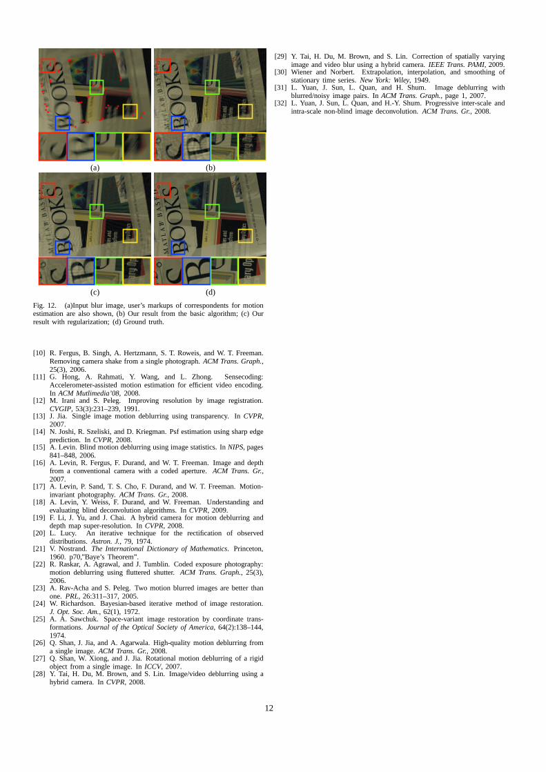
Figure 11 and Figure 12 show more real examples with zoom-in motion and rotational motion respectively. The motion blurredmatrix HN is obtained by fitting the transformation matrix withuser markup as shown in Figure 11(a) and Figure 12(a) respec-tively. Eachhi is computed by assuming the motion is a uniformmotion. We show the deblurred results from our algorithm withoutand with regularization respectively in (b) and (c). The groundtruth image is shown in (d) for comparisons. We note that our realexamples contains more ringing artifacts than synthetic examples.This is due to small estimation errors inhi. The effects of imagenoise in our real examples are not as significant as in our synthetic

9

0

5

10

15

20

25

30

35

40

45

50

1 2 3 4 5 6 7 8 9 10 11 12 13 14 15

Input

Basic

Reg.

Test case

RM

S E

rro

rs

0

5

10

15

20

25

30

35

40

45

50

1 2 3 4 5 6 7 8 9 10 11 12 13 14 15

Input

Basic

Reg.

RM

S E

rro

rs

Test case

0

5

10

15

20

25

30

35

40

45

50

1 2 3 4 5 6 7 8 9 10 11 12 13 14 15

Input

Basic

Reg.

Test case

RM

S E

rro

rs

Mandrill Lena Cameraman

0

5

10

15

20

25

30

35

40

45

50

1 2 3 4 5 6 7 8 9 10 11 12 13 14 15

Input

Basic

Reg.

Test case

RM

S E

rro

rs

0

5

10

15

20

25

30

35

40

45

50

1 2 3 4 5 6 7 8 9 10 11 12 13 14 15

Input

Basic

Reg.

Test case

RM

S E

rro

rs

Fruits PAMI

Fig. 9. RMS pixel errors for different example and test cases in our synthetic examples. We compare theRMS of the input blur image (blue), the deblurredimage using basic Projective Motion RL (red) and the deblurred image using Projective Motion RL with (Total Variation) regularization (green). These testcases show that our Projective Motion RL is effective in dealing with rigid spatially varying motion blur.All tested images and results are available in thesupplemental materials.

test case because long exposure time minimized the amount ofimage noise and also the motions in our real examples are not aslarge as in our synthetic example.

VIII. D ISCUSSION ANDCONCLUSION

This paper has introduced two contributions to motion deblur-ring. The first is our formulation of the motion blur as an inte-gration of the scene that has undergone a projective motion path.While a straight-forward representation, we have found that thisformulation is not used in image deblurring. The advantages ofthis motion blur model is that it is kernel-free and offers a compactrepresentation for spatially varying blur due to projective motion.In addition, this kernel free formulation is intuitive with regards tothe physical phenomena causing the blur. Our second contributionis an extension to the RL deblurring algorithm to incorporate ourmotion blur model in a correction algorithm. We have outlined thebasic algorithm as well as details on incorporating state-of-the-artregularization. Our experimental result section has demonstratedthe effectiveness of our approach on a variety of examples.

In this section, we discuss issues related to our ProjectiveMotion Blur Model and our Projective Motion RL algorithm. Inparticular, we will discuss the pros and cons of our ProjectiveMotion Blur Model in comparing with conventional PSF repre-sentation. We will also discuss limitations of our approaches andsuggest some future research direction based on our model.

A. Conventional PSF representation versus Projective Model BlurModel

For global in-plane motion blur, the conventional representationof the PSF consists of a square matrix (i.e. kernel) that describesthe contributions of pixels within a local neighborhood. This rep-resentation has several advantages. First, it is easy to understandand provides an intuitive represents of “point spread” about apoint. Second, this model handles other global blurring effects

(e.g. defocus) and motion blur in a unified representation, whileour representation only targets motion blur. Third, by assumingthe motion blur is globally the same, image deconvolution canbe done in the frequency domain, while our Projective MotionRL algorithm can only be done in the spatial domain. Thisconventional representation, however, is not suitable for dealingwith spatially varying motion blur. For such cases, our ProjectiveMotion RL formulation becomes advantageous.

B. Other deblurring methods based on Projective Motion Model

While we have developed our deblurring algorithm basedon Richardson-Lucy, we note that other algorithmic frameworkfor motion deblurring could be used. For example, using ourprojective motion model, we could construct a system of linearequations in the form ofy = Ax + n where each row ofAis the contribution of the pixels in the unblurred imagex tothe corresponding blurred pixely. The termn could be usedto represent noise. This would require a matrix of dimension(N ×N), whereN is the size of the image. While such a massivelinear system is undesirable, the sparse nature of the matrix wouldallow sparse matrix approaches such as that demonstrated byLevin et al. [16]. Such methods do not requireA to be explicitlyrepresented, only the the evaluation of the matrix product to beconstructed. How to incorporate regularization into such a methodis not entirely straight-forward and one reason we have workedfrom the RL algorithm.

C. Limitations

Our projective motion RL algorithm has several limitationsimilar to other deblurring algorithms. A fundamental limitationto our algorithm is that the high frequency details that havebeen lost during the motion blur process cannot be recovered.Our algorithm can only recover the “hidden” details that remaininside the motion blur images. Another limitation is that our

10

(a) (b)

(c) (d)

Fig. 10. Image deblurring using globally invariant kernels. (a) Input froma hybrid camera (courtesy of [29]) where the high-frame-rate low resolutionimages are also shown; (b) Result generated by [3](Standard RL algorithmfrom Matlab); (c) Result from our Projective Motion RL with regularization.(d) The ground truth sharp image. Close-up views and the estimated globalblur kernels are also shown.

approach does not deal with moving or deformable objects orscene with significant depth variation. A preprocessing step toseparate moving objects or depth layers out from backgroundis necessary to deal with this limitation. Other limitations of ourapproach include the problem of pixel color saturations and severeimage noise.

D. Running Time Analysis

Our current implementation takes about 15 minutes to run500 iterations on an image size512 × 512 with Intel(R)CPUL2400@1.66Ghz and 512MB of RAM. The running time ofour algorithm depends on several factors, including image size|I |, number of discrete samplingN (number of homographies)and the number of iterationsT . Hence, the running time of ouralgorithm isO(|I |NT ). We note that most of our running time inour implementation is spent in the bicubic interpolation processto generate the synthetic blur image and to integrate the residualerrors. One possible solution to speed up our process is to useGPU for the projective transformation of eachdt.

E. Future Directions

There are several major future directions of this work. One isto explore other existing algorithms and hardware (e.g. coded ex-posure and coded aperture) to use this blur formulation instead ofassuming a global PSF. Another important direction is to considerhow to use our framework to perform blind-deconvolution wherethe rigid motion is unknown. Estimating a piecewise projectivecamera motion is very different from estimating the global PSF in

++

++

++

++

++

++

++

++

++

++

++

++

++

++

++ +

++++

+

(a) (b)

(c) (d)

Fig. 11. (a)Input blur image, user’s markups of correspondents for motionestimation are also shown, (b) Our result from the basic algorithm; (c) Ourresult with regularization; (d) Ground truth.

a conventional deblurring algorithm. However, if we assume themotion satisfied our Projective Motion Blur Model, we may beable to impose constrains that can estimate the projective motionpath. Other possible directions is to include more than one motionblur images, e.g. noisy and blurry image pairs, for the estimationof the projective motion.

Another potential research direction is on about moving ob-ject/depth layer separation to extend our algorithm to deal withthe limitation discussed above. In order to apply our algorithmto a moving object, we not only need to segment the movingobject out from background, but we have to segment the movingobject in a piecewise manner such that each piece of segmentitself satisfied our Projective Motion Blur Model. For this kindof segmentation, we cannot use traditional “hard” segmentationalgorithm, since for the boundaries of motion blurred object isa fractional boundary much like that used in image matting.However, unlike conventional image matting, we can imposeadditional constraints regarding object’s motion.

REFERENCES

[1] A. Agrawal and R. Raskar. Resolving objects at higher resolution froma single motion-blurred image. InCVPR, 2007.

[2] J. Bardsley, S. Jefferies, J. Nagy, and R. Plemmons. Blind iterativerestoration of images with spatially-varying blur. InOptics Express,pages 1767–1782, 2006.

[3] M. Ben-Ezra and S. Nayar. Motion Deblurring using Hybrid Imaging.In CVPR, volume I, pages 657–664, Jun 2003.

[4] M. Ben-Ezra and S. Nayar. Motion-based Motion Deblurring.IEEETrans. PAMI, 26(6):689–698, Jun 2004.

[5] D. A. Bini, N. J. Higham, and B. Meini. Algorithms for the matrix p’throot. Numerical Algorithms, 39(4):349–378, 2005.

[6] J. Chen and C. K. Tang. Robust dual motion deblurring. InCVPR,2008.

[7] S. Cho, Y. Matsushita, and S. Lee. Removing non-uniform motion blurfrom images. InICCV, 2007.

[8] S. Dai and Y. Wu. Motion from blur. InCVPR, 2008.[9] N. Dey, L. Blanc-Fraud, C. Zimmer, Z. Kam, P. Roux, J. Olivo-Marin,

and J. Zerubia. A deconvolution method for confocal microscopy withtotal variation regularization. InIEEE International Symposium onBiomedical Imaging: Nano to Macro, 2004.

11

++

++

++

++

++

++

++

++

++

+++

+

++++

+

+

++

+

+

+

+

++

++

++

++

++

+

+

++

++

++

++

(a) (b)

(c) (d)

Fig. 12. (a)Input blur image, user’s markups of correspondents for motionestimation are also shown, (b) Our result from the basic algorithm; (c) Ourresult with regularization; (d) Ground truth.

[10] R. Fergus, B. Singh, A. Hertzmann, S. T. Roweis, and W. T. Freeman.Removing camera shake from a single photograph.ACM Trans. Graph.,25(3), 2006.

[11] G. Hong, A. Rahmati, Y. Wang, and L. Zhong. Sensecoding:Accelerometer-assisted motion estimation for efficient video encoding.In ACM Mutlimedia’08, 2008.

[12] M. Irani and S. Peleg. Improving resolution by image registration.CVGIP, 53(3):231–239, 1991.

[13] J. Jia. Single image motion deblurring using transparency. InCVPR,2007.

[14] N. Joshi, R. Szeliski, and D. Kriegman. Psf estimation using sharp edgeprediction. InCVPR, 2008.

[15] A. Levin. Blind motion deblurring using image statistics. InNIPS, pages841–848, 2006.

[16] A. Levin, R. Fergus, F. Durand, and W. T. Freeman. Image and depthfrom a conventional camera with a coded aperture.ACM Trans. Gr.,2007.

[17] A. Levin, P. Sand, T. S. Cho, F. Durand, and W. T. Freeman. Motion-invariant photography.ACM Trans. Gr., 2008.

[18] A. Levin, Y. Weiss, F. Durand, and W. Freeman. Understanding andevaluating blind deconvolution algorithms. InCVPR, 2009.

[19] F. Li, J. Yu, and J. Chai. A hybrid camera for motion deblurring anddepth map super-resolution. InCVPR, 2008.

[20] L. Lucy. An iterative technique for the rectification of observeddistributions. Astron. J., 79, 1974.

[21] V. Nostrand. The International Dictionary of Mathematics. Princeton,1960. p70,”Baye’s Theorem”.

[22] R. Raskar, A. Agrawal, and J. Tumblin. Coded exposure photography:motion deblurring using fluttered shutter.ACM Trans. Graph., 25(3),2006.

[23] A. Rav-Acha and S. Peleg. Two motion blurred images are better thanone. PRL, 26:311–317, 2005.

[24] W. Richardson. Bayesian-based iterative method of image restoration.J. Opt. Soc. Am., 62(1), 1972.

[25] A. A. Sawchuk. Space-variant image restoration by coordinate trans-formations. Journal of the Optical Society of America, 64(2):138–144,1974.

[26] Q. Shan, J. Jia, and A. Agarwala. High-quality motion deblurring froma single image.ACM Trans. Gr., 2008.

[27] Q. Shan, W. Xiong, and J. Jia. Rotational motion deblurring of a rigidobject from a single image. InICCV, 2007.

[28] Y. Tai, H. Du, M. Brown, and S. Lin. Image/video deblurring using ahybrid camera. InCVPR, 2008.

[29] Y. Tai, H. Du, M. Brown, and S. Lin. Correction of spatially varyingimage and video blur using a hybrid camera.IEEE Trans. PAMI, 2009.

[30] Wiener and Norbert. Extrapolation, interpolation, and smoothing ofstationary time series.New York: Wiley, 1949.

[31] L. Yuan, J. Sun, L. Quan, and H. Shum. Image deblurring withblurred/noisy image pairs. InACM Trans. Graph., page 1, 2007.

[32] L. Yuan, J. Sun, L. Quan, and H.-Y. Shum. Progressive inter-scale andintra-scale non-blind image deconvolution.ACM Trans. Gr., 2008.

12

T7

T5

T11

T14

T15 Blurred images Result from basic Projective Motion RL Results with regularization included

Fig. 13. In this figure, we show several examples of our test cases in Figure 9. The whole set of test cases and results are submitted in supplementalmaterials.

13