ping yu - university of hong kongweb.hku.hk/~pingyu/6066/slides/ln2_constrained...

Constrained Optimization

Ping Yu

Department of EconomicsUniversity of Hong Kong

Ping Yu (HKU) Constrained Optimization 1 / 38

1 Equality-Constrained OptimizationLagrange MultipliersCaveats and Extensions

2 Inequality-Constrained OptimizationKuhn-Tucker ConditionsThe Constraint Qualification


Overview of This Chapter

We will study the first order necessary conditions for an optimization problem withequality and/or inequality constraints.

The former is often called the Lagrange problem and the latter is called theKuhn-Tucker problem (or nonlinear programming).

We will not discuss the unconstrained optimization problem separately but treat itas a special case of the constrained problem because the unconstrained problemis rare in economics.


Maximum/Minimum and Maximizer/Minimizer

A function f : X !R has a global maximizer at x� if f (x�)� f (x) for all x 2 X andx 6= x�. Similarly, the function has a global minimizer at x� if f (x�)� f (x) for allx 2 X and x 6= x�.

If the domain X is a metric space, usually a subset of Rn, then f is said to have alocal maximizer at the point x� if there exists r > 0 such that f (x�)� f (x) for allx 2 Br (x�)\Xnfx�g, where Br (x�) is an open ball with center x� and radius r .Similarly, the function has a local minimizer at x� if f (x�)� f (x) for allx 2 Br (x�)\Xnfx�g.In both the global and local cases, the value of the function at a maximizer iscalled the maximum of the function and the value of the function at a minimizer iscalled the minimum of the function.- The maxima and minima (the respective plurals of maximum and minimum) arecalled optima (the plural of optimum), and the maximizer and minimizer are calledthe optimizer. The optimizer and optimum without any qualifier means the globalones. [Figure here]- A global optimizer is always a local optimizer but the converse is not correct.

In both the global and local cases, the concept of a strict optimum and a strictoptimizer can be defined by replacing weak inequalities by strict inequalities.


Figure: Local and Global Maxima and Minima for cos(3πx)/x , 0.1� x � 1.1


Notations

The problem of maximization is usually stated as

maxx

f (x)

s.t. x 2 X ,

where "s.t." is a short for "subject to",1 and X is called the constraint set or feasibleset.

The maximizer is denoted as

argmaxff (x)jx 2 Xg or argmaxx2X

f (x),

where "arg" is a short for "arguments".

The difference between the Lagrange problem and Kuhn-Tucker problem lies inthe definition of X .

1"s.t." is also a short for "such that" in some books.Ping Yu (HKU) Constrained Optimization 5 / 38

Equality-Constrained Optimization

Equality-Constrained Optimization


Equality-Constrained Optimization Lagrange Multipliers

Consumer’s Problem

In microeconomics, a consumer faces the problem of maximizing her utility subjectto the income constraint:

maxx1,x2

u(x1,x2)

s.t. p1x1+p2x2�y = 0

If the indifference curves (i.e., the sets of points (x1,x2) for which u(x1,x2) is aconstant) are convex to the origin, and the indifference curves are nice andsmooth, then the point (x�1 ,x

�2) that solves the maximization problem is the point at

which the indifference curve is tangent to the budget line as given in the followingfigure.



Figure: Utility Maximization Problem in Consumer Theory



Economic Condition for Maximization

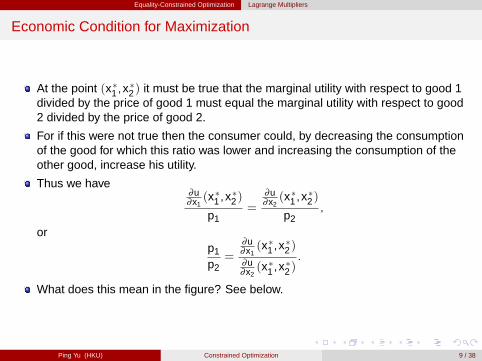
At the point (x�1 ,x�2) it must be true that the marginal utility with respect to good 1

divided by the price of good 1 must equal the marginal utility with respect to good2 divided by the price of good 2.

For if this were not true then the consumer could, by decreasing the consumptionof the good for which this ratio was lower and increasing the consumption of theother good, increase his utility.

Thus we have∂u∂x1(x�1 ,x

�2)

p1=

∂u∂x2(x�1 ,x

�2)

p2,

orp1

p2=

∂u∂x1(x�1 ,x

�2)

∂u∂x2(x�1 ,x

�2).

What does this mean in the figure? See below.



Mathematical Arguments

Let xu2 be the function that defines the indifference curve through the point

(x�1 ,x�2), i.e.,

u(x1,xu2 (x1))� u � u(x�1 ,x

�2).

Now, totally differentiating this identity gives

∂u∂x1

(x1,xu2 (x1))+

∂u∂x2

(x1,xu2 (x1))

dxu2

dx1(x1) = 0.

That is,dxu

2dx1

(x1) = �∂u∂x1(x1,xu

2 (x1))

∂u∂x2(x1,xu

2 (x1)).

Given that xu2 (x

�1) = x�2 , the slope of the indifference curve at the point (x�1 ,x

�2)

dxu2

dx1(x�1) = �

∂u∂x1(x�1 ,x

�2)

∂u∂x2(x�1 ,x

�2).

Also, the slope of the budget line is � p1p2

. Combining these two results again givesthe result in the last slide.



Necessary Conditions for Maximization

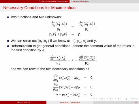
Two functions and two unknowns:

∂u∂x1(x�1 ,x

�2)

p1=

∂u∂x2(x�1 ,x

�2)

p2,

p1x�1 +p2x�2 = y .

We can solve out (x�1 ,x�2) if we know u(�, �), p1, p2 and y .

Reformulation to get general conditions: denote the common value of the ratios inthe first condition by λ ,

∂u∂x1(x�1 ,x

�2)

p1= λ =

∂u∂x2(x�1 ,x

�2)

p2,

and we can rewrite the two necessary conditions as

∂u∂x1

(x�1 ,x�2)�λp1 = 0,

∂u∂x2

(x�1 ,x�2)�λp2 = 0,

y �p1x�1 �p2x�2 = 0.



Lagrangian

Define the Lagrangian as

L (x1,x2,λ ) = u(x1,x2)+λ (y �p1x1�p2x2).

Calculate ∂L∂x1

, ∂L∂x2

, and ∂L∂λ

, and set the results equal to zero we obtain exactly thethree equations in the last slide.

Three equations and three unknowns, so we can solve out (x�1 ,x�2 ,λ

�) in principle.

λ is the new artificial or auxiliary variable, and is commonly called Lagrangemultiplier.



Joseph-Louis Lagrange (1736-1813), Italian2

2but worked at Berlin and Paris during most of his life.Ping Yu (HKU) Constrained Optimization 13 / 38


General Necessary Conditions for Maximization

Suppose that we have the following maximization problem

maxx1,�� ,xn

f (x1, � � � ,xn)

s.t. g(x1, � � � ,xn) = c

LetL (x1, : : : ,xn,λ ) = f (x1, : : : ,xn)+λ (c�g(x1, : : : ,xn)).

If (x�1 , : : : ,x�n) solves this maximization problem, there is a value of λ , say λ

� suchthat

∂L

∂xi(x�1 , : : : ,x

�n ,λ

�) = 0, i = 1, : : : ,n, (1)

∂L

∂λ(x�1 , : : : ,x

�n ,λ

�) = 0. (2)



More Explanations on the Necessary Conditions

The conditions (1) are precisely the first order conditions for choosing x1, : : : ,xn tomaximize L , once λ

� has been chosen.

From conditions (1), there are two equivalent ways to interpret the constrainedmaximization problem.- The decision maker must satisfy g(x1, : : : ,xn) = c and that he should chooseamong all points that satisfy this constraint the point at which f (x1, : : : ,xn) isgreatest.- The decision maker chooses any point he wishes but that for each unit by whichhe violates the constraint g(x1, : : : ,xn) = c we shall take away λ units from hispayoff.

We must be careful to choose λ to be the correct value.

If we choose λ too small, the decision maker may choose to violate his constraint.E.g., if we made the penalty for spending more than the consumer’s income verysmall the consumer would choose to consume more goods than he could affordand to pay the penalty in utility terms.

On the other hand, if we choose λ too large the decision maker may violate hisconstraint in the other direction. E.g., the consumer would choose not to spendany of his income and just receive λ units of utility for each unit of his income.



Multiple Constraints

The technique above can be extended to multiple constraints case:

maxx1,�� ,xn

f (x1, � � � ,xn)

s.t. g1(x1, � � � ,xn) = c1,

...

gm(x1, � � � ,xn) = cm,

where m � n or m < n (why?).The Lagrangian

L (x,λ ) = f (x)+λ � (c�g(x)), (3)where x = (x1, : : : ,xn)0, λ = (λ 1, � � � ,λ m)0, and c and g are similarly defined.If x� = (x�1 , : : : ,x

�n)0 solves (3), there are values of λ , say λ

� = (λ �1, : : : ,λ�m)0 such

that∂L

∂xi(x�,λ �) = 0, i = 1, : : : ,n

∂L

∂λ j(x�,λ �) = 0, j = 1, � � � ,m,

which are labeled as "first order conditions" or "FOCs" for the correspondingmaximization problem.The FOCs are the set of conditions which a solution to the maximization problemmust satisfy, so are actually the first order necessary conditions .


Equality-Constrained Optimization Caveats and Extensions

Existence of Maximizer

We have not even claimed that there necessarily is a solution to the maximizationproblem.

One example of an unconstrained problem with no solution is

maxx

2x ,

maximizing over the choice of x the function 2x . Clearly the greater we make x thegreater is 2x , and so, since there is no upper bound on x there is no maximum.

Thus we might want to restrict maximization problems to those in which wechoose x from some bounded set. Again, this is not enough.

Consider the problemmax

0�x�11/x .

The smaller we make x the greater is 1/x and yet at zero 1/x is not even defined.

We could define the function to take on some value at zero, say 7. But then thefunction would not be continuous. Or we could leave zero out of the feasible set forx , say 0< x � 1. Then the set of feasible x is not closed.



Weierstrass Theorem

We shall restrict maximization problems to those in which we choose x tomaximize some continuous function from some closed and bounded set (which iscompact from the Heine-Borel Theorem).

Is there anything else that could go wrong? No. The following result says that ifthe function to be maximized is continuous and the set over which we arechoosing is both closed and bounded, i.e., is compact, then there is a solution tothe maximization problem.

Theorem (The Weierstrass Theorem)

Let S be a compact set and f : S !R be continuous. Then there is some x� in S atwhich the function is maximized. More precisely, there is some x� in S such thatf (x�)� f (x) for any x in S.

We will give an example later.



Karl T.W. Weierstrass (1815-1897), German3

3cited as the "father of modern analysis", leaving university without a degree.Ping Yu (HKU) Constrained Optimization 19 / 38


Extension to Nonequality Constraints

In defining the compact sets in the Weierstrass theorem, we typically useinequalities, such as x � 0.

However, we did not consider such constraints in the above discussion, but ratherconsidered only equality constraints.

However, even in the example of utility maximization at the beginning of thissection, there were implicitly constraints on x1 and x2 of the form

x1 � 0, x2 � 0.

We shall return to this question in the next section.



Extension to Minimization Problem and Unconstrained Problem

We could have transformed the minimization problem into a maximization problemby simply multiplying the objective function by �1.

That is, if we wish to minimize f (x) we could do so by maximizing �f (x).

As an exercise write out the necessary conditions for the case that we wanted tominimize u(x) in the consumer’s problem.

Notice that if x�1 , x�2 , and λ satisfy the original equations then x�1 , x�2 , and �λ

satisfy the new equations. Thus we cannot tell whether there is a maximum at (x�1 ,x�2) or a minimum.

This corresponds to the fact that in the case of a function of a single variable overan unconstrained domain at a maximum we require the first derivative to be zero,but that to know for sure that we have a maximum we must look at the secondderivative which will be discussed in the next chapter.

For the unconstrained problem, set λ� = 0, i.e., since no constraints exist, no

penalty is imposed on constraints.


Inequality-Constrained Optimization

Inequality-Constrained Optimization(Nonlinear Programming)


Inequality-Constrained Optimization Kuhn-Tucker Conditions

Introduction to Nonlinear Programming

Formulation of a simple nonlinear programming problem:

maxx

f (x)

s.t. x � 0,

where dim(x) = 1 for simplicity.

Without the constraint x � 0, the FOC for the maximization problem is dfdx (x

�) = 0.

When the inequality constraint is added in, either the solution could occur whenx� > 0 or it could occur when x� = 0.

When x� > 0, the FOC should still be dfdx (x

�) = 0. When x� = 0, the necessarycondition should be

dfdx(x�)� 0.(why?)



Figure: Illustration of Why dfdx (x

�)� 0 When x� = 0



Nonlinear Programming with Possible Corner Solution

So the FOC isdfdx(x�)

�� 0,= 0,

if x� = 0,if x� > 0,

which can be expressed in a compact form as in the following theorem.

Theorem

Suppose that f : R!R is a C1 function. Then, if x� maximizes f (x) over all x � 0, x�

satisfies

dfdx(x�) � 0

x�dfdx(x�) = 0

x� � 0



Reformulation of the FOCs

As in the equality-constrained problem, we introduce a Lagrange multiplier.

If we form the LagrangianL (x ,λ ) = f (x)+λx ,

then we can express these FOCs as (check!)

∂L

∂x(x�,λ �) =

dfdx(x�)+λ

� = 0,

∂L

∂λ(x�,λ �) = x� � 0,

λ� � 0,λ �

∂L

∂λ(x�,λ �) = λ

�x� = 0.



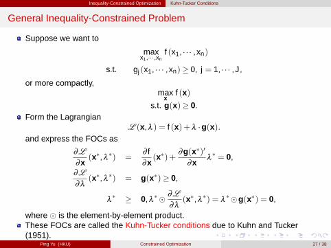
General Inequality-Constrained Problem

Suppose we want to

maxx1,�� ,xn

f (x1, � � � ,xn)

s.t. gj (x1, � � � ,xn)� 0, j = 1, � � � ,J,or more compactly,

maxx

f (x)

s.t. g(x)� 0.Form the Lagrangian

L (x,λ ) = f (x)+λ �g(x).and express the FOCs as

∂L

∂x(x�,λ �) =

∂ f∂x(x�)+

∂g(x�)0

∂xλ� = 0,

∂L

∂λ(x�,λ �) = g(x�)� 0,

λ� � 0,λ �� ∂L

∂λ(x�,λ �) = λ

��g(x�) = 0,

where � is the element-by-element product.These FOCs are called the Kuhn-Tucker conditions due to Kuhn and Tucker(1951).



H.W.Kuhn (1925-2014, Princeton) A.W. Tucker (1905-1995, Princeton)4

4Albert W. Tucker is the supervisor of John Nash, the Nobel Prize winner in Economics in 1994, and LloydShapley, the Nobel Prize winner in Economics in 2012.



Mixed Constrained Problem

Combine the equality-constrained and inequality-constrained problem to definethe mixed constrained problem:

maxx1,�� ,xn

f (x1, � � � ,xn)

s.t. gj (x1, � � � ,xn)� 0, j = 1, � � � ,J,hk (x1, � � � ,xn) = 0, k = 1, � � � ,K ,

or more compactly,max

xf (x)

s.t. g(x)� 0,h(x) = 0,

where K � n.

The term "mixed constrained problem" is only for convenience because anyequality constraint can be transformed to two inequality constraints, e.g.,hk (x) = 0 is equivalent to hk (x)� 0 and hk (x)� 0.

Form the Lagrangian

L (x,λ ,µ) = f (x)+λ �g(x)+ µ �h(x).



Theorem of Kuhn-Tucker

Theorem (Theorem of Kuhn-Tucker)

Suppose that f : Rn !R, g : Rn !RJ and h : Rn !RK are C1 functions. Then, if x�

maximizes f (x) over all x satisfying the constraints g(x)� 0 and h(x) = 0, and if x�

satisfies the nondegenerate constraint qualification (NDCQ) as will be discussedbelow, then there exists a vector (λ �,µ�) such that (x�,λ �,µ�) satisfies theKuhn-Tucker conditions given as follows:

∂L∂x (x

�,λ �,µ�) = 0, ∂L∂ µ(x�,λ �,µ�) = h(x�) = 0,

∂L∂λ(x�,λ �,µ�) = g(x�)� 0, λ

� � 0,λ�� ∂L

∂λ(x�,λ �,µ�) = λ

��g(x�) = 0.

The x�’s that satisfy the Kuhn-Tucker conditions are called the critical points of L .

Usually, critical points mean the points that satisfy the FOCs; the Kuhn-Tuckerconditions are a special group of FOCs.

Parallel to Lagrange multipliers in the Lagrange problem, (λ �,µ�) are calledKuhn-Tucker multipliers.

Finally, note that the Kuhn-Tucker conditions are necessary conditions for "local"optima, and of course are also necessary conditions for global optima.


Inequality-Constrained Optimization The Constraint Qualification

Nondegenerate Constraint Qualification

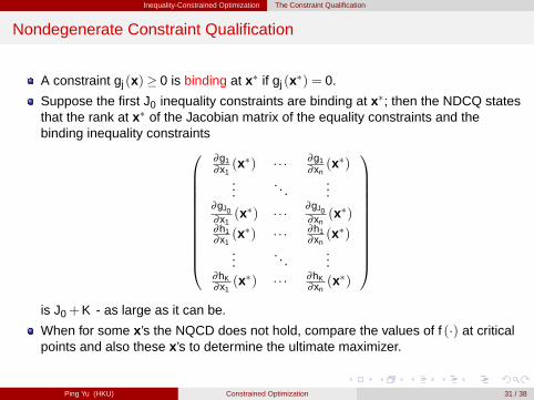
A constraint gj (x)� 0 is binding at x� if gj (x�) = 0.

Suppose the first J0 inequality constraints are binding at x�; then the NDCQ statesthat the rank at x� of the Jacobian matrix of the equality constraints and thebinding inequality constraints0BBBBBBBBBBB@

∂g1∂x1(x�) � � � ∂g1

∂xn(x�)

.... . .

...∂gJ0∂x1

(x�) � � � ∂gJ0∂xn

(x�)∂h1∂x1(x�) � � � ∂h1

∂xn(x�)

.... . .

...∂hK∂x1(x�) � � � ∂hK

∂xn(x�)

1CCCCCCCCCCCAis J0+K - as large as it can be.

When for some x’s the NQCD does not hold, compare the values of f (�) at criticalpoints and also these x’s to determine the ultimate maximizer.



Failure of the Constraint Qualification

Example

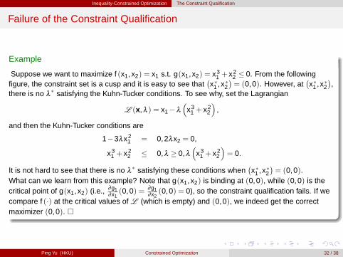
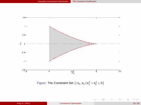
Suppose we want to maximize f (x1,x2) = x1 s.t. g(x1,x2) = x31 + x2

2 � 0. From the followingfigure, the constraint set is a cusp and it is easy to see that

�x�1 ,x

�2

�= (0,0). However, at

�x�1 ,x

�2

�,

there is no λ� satisfying the Kuhn-Tucker conditions. To see why, set the Lagrangian

L (x,λ ) = x1�λ

�x3

1 + x22

�,

and then the Kuhn-Tucker conditions are

1�3λx21 = 0,2λx2 = 0,

x31 + x2

2 � 0,λ � 0,λ�

x31 + x2

2

�= 0.

It is not hard to see that there is no λ� satisfying these conditions when

�x�1 ,x

�2

�= (0,0).

What can we learn from this example? Note that g(x1,x2) is binding at (0,0), while (0,0) is thecritical point of g(x1,x2) (i.e., ∂g1

∂x1(0,0) = ∂g1

∂x2(0,0) = 0), so the constraint qualification fails. If we

compare f (�) at the critical values of L (which is empty) and (0,0), we indeed get the correctmaximizer (0,0). �



Figure: The Constraint Set�(x1,x2)jx3

1 + x22 � 0



An Illustrating Example of Finding the Maximizer

Example

max x21 +(x2�5)2 s.t. x1 � 0, x2 � 0, and 2x1+ x2 � 4.

Solution

First, since the objective function is continuous and the constraint set is compact (why?), by theWeierstrass theorem, the maximizer exists. We then check the NDCQ. g1(x) = x1, g2(x) = x2 andg3(x) = 4�2x1�x2, so the Jacobian of the constraint functions is0@ 1 0

0 1�2 �1

1A ,whose any one or two rows are linearly independent. Since at most two of the three constraintscan be binding at any one time, the NDCQ holds at any solution candidate.The Lagrangian is

L (x ,λ ,µ) = x21 +(x2�5)2+λ 1x1+λ 2x2+λ 3(4�2x1�x2),

and the Kuhn-Tucker conditions are

2x1+λ 1�2λ 3 = 0, 2(x2�5)+λ 2�λ 3 = 0,

x1 � 0, x2 � 0, 4�2x1�x2 � 0,λ 1 � 0,λ 2 � 0,λ 3 � 0,

λ 1x1 = 0, λ 2x2 = 0, λ 3(4�2x1�x2) = 0.



Solution (continue)

Totally eight possibilities depending whether λ j = 0 or not, j = 1,2,3.(i) λ 1 > 0,λ 2 > 0 and λ 3 > 0=) x1 = 0,x2 = 0, and 2x1+ x2 = 4. Impossible.(ii) λ 1 = 0,λ 2 > 0 and λ 3 > 0=) x1 � 0,x2 = 0, and 2x1+ x2 = 4. So (x1,x2) = (2,0). From4�2λ 3 = 0 and �10+λ 2�λ 3 = 0, we have (λ 1,λ 2,λ 3) = (0,12,2).(iii) λ 1 > 0,λ 2 = 0 and λ 3 > 0=) x1 = 0,x2 � 0, and 2x1+ x2 = 4. So (x1,x2) = (0,4). Fromλ 1�2λ 3 = 0 and �2�λ 3 = 0, we have (λ 1,λ 2,λ 3) = (�2,0,�4). Impossible.(iv) λ 1 = λ 2 = 0 and λ 3 > 0=) x1 � 0,x2 � 0, and 2x1+ x2 = 4. So from2x1�2λ 3 = 0,2(x2�5)�λ 3 = 0, and 2x1+x2 = 4, we have (x1,x2) = (�2/5,24/5) . Impossible.(v) λ 1 > 0,λ 2 > 0 and λ 3 = 0=) x1 = 0,x2 = 0, and 2x1+ x2 � 4. So (x1,x2) = (0,0). Fromλ 1 = 0 and �10+λ 2 = 0, we have (λ 1,λ 2,λ 3) = (0,10,0). Impossible.(vi) λ 1 = λ 3 = 0,λ 2 > 0=) x1 � 0,x2 = 0, and 2x1+ x2 � 4. From 2x1 = 0 and �10+λ 2 = 0, wehave (x1,x2) = (0,0) and (λ 1,λ 2,λ 3) = (0,10,0).(vii) λ 1 > 0,λ 2 = λ 3 = 0=) x1 = 0,x2 � 0, and 2x1+ x2 � 4. So from λ 1 = 0 and 2(x2�5) = 0,we have (x1,x2) = (0,5) and (λ 1,λ 2,λ 3) = (0,0,0). Impossible.(viii) λ 1 = λ 2 = λ 3 = 0=) x1 � 0,x2 � 0, and 2x1+ x2 � 4. So from 2x1 = 0 and 2(x2�5) = 0,we have (x1,x2) = (0,5). Impossible.Candidate maximizers are (2,0) and (0,0). The objective function values at these two candidatesare 29 and 25, so (2,0) is the maximizer and the associated Lagrange multipliers are (0,12,2). �



Caution: Never blindly apply the Kuhn-Tucker conditions.

Figure: Intuitive Illustration of Example



A "Cookbook" Procedure of Optimization

Define the feasible set of the general mixed constrained maximization problem as

G =�

x 2Rnjg(x)� 0,h(x) = 0.

Step 1: Apply the Weierstrass theorem to show that the maximum exists. If thefeasible set G is compact, this is usually straightforward; if G is notcompact, truncate G to a compact set, say Go, such that there is apoint xo 2Go and f (xo)> f (x) for all x 2GnGo.

Step 2: Check whether the constraint qualification is satisfied. If not, denote theset of possible violation points as Q.

Step 3: Set up the Lagrangian and find the critical points. Denote the set ofcritical points as R.

Step 4: Check the value of f on Q[R to determine the maximizer ormaximizers.



Caution

It is quite often for practitioners to apply Step 3 directly to find the maximizer.Although this may work in most cases, it is possible to fail in some cases.

First, the Lagrangian may fail to have any critical points due to nonexistence ofmaximizers or failure of constraint qualification.

Second, even if the Lagrangian does have one or more critical points, this set ofcritical points need not contain the solution still due to these two reasons.

Let us repeat our caveat, "Never blindly apply the Kuhn-Tucker conditions"!

This cookbook procedure works well in most cases, especially when the set Q[Ris small, e.g., Q[R includes only a few points.

If this set is large, it is better to employ more necessary conditions (e.g., thesecond order conditions (SOCs)) to screen the points in Q[R.

Another solution is to employ sufficient conditions, i.e., as long as x� satisfiesthese conditions, it must be the maximizer.- Sufficient conditions are very powerful especially combined with the uniquenessresult because as long as we find one solution, it is the solution and we can stop.

These topics are the main theme of the next chapter.


ping yu - university of hong kongweb.hku.hk/~pingyu/6066/slides/ln2_constrained...

Documents