yu ma, kusum l. ailawadi, dinesh k. gauri, & dhruv …... american marketing association issn:...

18Journal of Marketing

Vol. 75 (March 2011), 18 –35

© 2011, American Marketing Association

ISSN: 0022-2429 (print), 1547-7185 (electronic)

Yu Ma, Kusum L. Ailawadi, Dinesh K. Gauri, & Dhruv Grewal

An Empirical Investigation of theImpact of Gasoline Prices onGrocery Shopping Behavior

The authors empirically examine the effect of gas prices on grocery shopping behavior using InformationResources Inc. panel data from 2006 to 2008, which track panelists’ purchases of almost 300 product categoriesacross multiple retail formats. The authors quantify the impact on consumers’ total spending and examine thepotential avenues for savings when consumers shift from one retail format to another, from national brands toprivate labels, from regular-priced to promotional products, and from higher to lower price tiers. They find asubstantial negative effect on shopping frequency and purchase volume and shifts away from grocery and towardsupercenter formats. A greater shift occurs from regular-priced national brands to promoted ones than to privatelabels, and among national brand purchasers, bottom-tier brands lose share, midtier brands gain share, and top-tier brand share is relatively unaffected. The analysis also controls for general economic conditions and shows thatgas prices have a much larger impact on grocery shopping behavior than broad economic factors.

Keywords: grocery expenditure, gas price effect, macroeconomic factors, retail format choice, promotions, privatelabel

Yu Ma is Assistant Professor, Department of Marketing, Business Eco-nomics, and Law, School of Business, University of Alberta (e-mail:[email protected]). Kusum L. Ailawadi is Charles Jordan 1911 TU’12Professor of Marketing, Tuck School of Business, Dartmouth College (e-mail: [email protected]). Dinesh K. Gauri is Assistant Pro-fessor of Marketing, Whitman School of Management, Syracuse Univer-sity (e-mail: [email protected]). Dhruv Grewal is Toyota Chair ofCommerce and Electronic Business and Professor of Marketing, BabsonCollege (e-mail: [email protected]). The authors thank InformationResources Inc. for providing the panel data used in this research and theAlberta School of Retailing for a research grant awarded to the firstauthor. They also thank Scott Fay, Peter Golder, Kevin Keller, and ScottNeslin for their helpful comments.

Macroeconomic conditions influence consumers’ atti-tudes, shopping behavior, and consumption. Althoughthese conditions are not controllable by manufactur-

ers and retailers, understanding how they affect consumersand how consumers respond to them is critical in guidingeffective managerial actions. This issue currently occupiescenter stage as the world economy tries to emerge from themost severe economic crisis in decades.

A small but rich body of literature in marketing exam-ines the impact of macroeconomic factors. One stream ofresearch describes how firms change advertising, innova-tion, and other “proactive” marketing activities during arecession and assesses the effectiveness of these actions(Deleersnyder et al. 2009; Frankenberger and Graham2003; Srinivasan, Rangaswamy, and Lilien 2005). Anotherstream studies the effect of business cycles and consumerconfidence on sales of durable goods (Allenby, Jen, andLeone 1996; Deleersnyder et al. 2004; Kumar, Leone, andGaskins 1995) and private labels (Lamey et al. 2007). Both

streams of research are typically conducted at an aggregatelevel, with industry-, firm-, or product category–level salesdata. Yet change in consumer behavior is at the root of whythese macroeconomic variables affect sales and firm perfor-mance. Therefore, it is important to conduct a more disag-gregate analysis (Deleersnyder et al. 2004) and understandhow consumers react to changes in macroeconomic factors(Grewal, Levy, and Kumar 2009).

An underlying theme in the literature is the notion thatconsumers’ response to macroeconomic factors is a func-tion of not just their ability to buy (as measured by currentand expected future income) but also their willingness tobuy (as measured by attitudes, sentiment, and so on)(Katona 1975). Conventional wisdom maintains that macro-economic factors and consumer sentiment have an impacton durable goods sales because purchases of such productsare discretionary and can be postponed when willingness tobuy is low whereas nondurable products, such as groceries,are less affected because they cannot be postponed (Deleer-snyder et al. 2004; Lamey et al. 2007).

The focus of the current research is on a macroeco-nomic factor that is qualitatively different from businesscycles and consumer sentiment and has been prominent inrecent years—namely, the price of gasoline. Since 2006, theprice of a gallon of regular gasoline has varied widely, fromlows of just over $2.00 to highs of more than $4.00. Gaso-line demand is fairly inelastic (Brons et al. 2008; Greeninget al. 1995), so expenditure on gas goes up in accordancewith its price. A U.S. household earning a median incomespent 11.5% of that income on gas in July 2008, up from4.6% in 2003 (The Wall Street Journal 2008). When theprice of gas increases sharply, consumers have less dispos-

able income, feel significant financial hardship, becomemore price conscious, and must find ways to reduce spend-ing in other areas (Du and Kamakura 2008; Jacobe 2006).Consistent with this, Hamilton (2008) notes in his recentreview of oil and the economy that the key mechanismwhereby energy price shocks affect the economy is througha disruption in spending on goods and services other thanenergy.

Thus, the impact of gas prices on consumer shoppingbehavior derives not just from psychological willingness tobuy but also from the immediate economic ability to buy.Grocery products individually cost little relative to overallincome. However, after housing and transportation, theyform the largest percentage of U.S. households’ annualexpenditures. For example, expenditure on food at home forthe average household was 5.6% of total income after taxesin 2007, exceeding other expense categories such asapparel, entertainment, and health care (Bureau of LaborStatistics 2007). Furthermore, grocery shopping is done fre-quently, generally more than once a week, so there is plentyof opportunity to make adjustments in purchases. There-fore, expenditures on grocery products provide a substantialand flexible means to adjust spending in response to unex-pected changes in discretionary income. In summary, gro-cery products may be relatively immune to general eco-nomic conditions and business cycles, but this is not likelyto be the case with rising gas prices.

However, there is little systematic research on theimpact of gas prices on consumers’ shopping behavior. Anexception is the work of Gicheva, Hastings, and Villas-Boas(2010); using Consumer Expenditure Survey data (Bureauof Labor Statistics 2007), they find that expenditures onfood outside the home decrease by 56% and expenditureson food purchased at grocery stores increase slightly with a100% increase in gas price. They also use sales data in fourfood categories from a California grocery chain to showthat consumers substitute away from regular shelf-priceproducts and toward promotional items to save money onoverall grocery expenditures.

The objective of our research is to provide a compre-hensive analysis of the impact of gas prices on consumers’grocery shopping behavior. Consumers can alter how muchthey purchase, how often they purchase, and how much theyspend on their purchases, which in turn is a function ofwhat they buy and where they buy it. We not only quantifythe impact on households’ shopping frequency, total pur-chase volume, and spending but also examine the avenuesthey use to save money on grocery shopping, such as shift-ing from one retail format to another, from national brandsto private labels, from regular-priced products to promo-tional purchases, and from higher-priced national brands tolower-priced ones. Such an analysis is important not onlyfor researchers and policy makers but also for manufactur-ers and retailers, which must determine the best way torespond to and perhaps preempt changes in shoppingbehavior in an era of “peak oil” and sustained volatility inenergy prices. As we discuss in the next section, theanswers are not obvious.

We conduct our analysis using a household panel dataset from Information Resources Inc. The data set captures

Empirical Investigation on Grocery Shopping Behavior / 19

grocery shopping information across multiple retail formatsof approximately 1000 panelists from a major U.S. metro-politan area. The data are from January 2006 to October2008 and span panelists’ purchases of almost 300 productcategories. We supplement these data with gas prices in thesame metropolitan area obtained from the Department ofEnergy Information Administration Web site. Some uniquefeatures of these data make them especially useful for ourresearch. First, we cover not just a few product categoriesbut rather the vast majority of consumer packaged goodsproducts purchased by consumers. Second, we cover boththe traditional grocery store and drugstore channels and theregular and supercenter stores of mass merchants (includingWal-Mart) and warehouse clubs. Third, substantial variationin gas prices occurred during the period of our data. Fourth,we control for general economic conditions to isolate andcontrast the impact of gas prices.

We organize the remainder of this article as follows: Inthe next section, we present the conceptual framework forour model and analysis, drawing on relevant literaturewhenever possible. Then, we discuss our data and method-ology. Following this, we present our empirical results anddiscuss the implications of our findings for researchers andmanagers.

Conceptual Development

Overview

Figure 1 depicts the framework that guides our expectationsand analysis. Gas prices affect consumers’ budget constraintbecause an increase in gas prices directly reduces the incomeavailable for other purchases, given the relative inability toreduce gas consumption in the short run. The budget con-straint requires consumers to reduce their total spending.They can do this by lowering their purchase volume (con-sumption) and/or by reducing the cost of their purchases.Cost can be reduced by shifting to less expensive retail for-mats, private label products or national brands on promo-tion, and/or lower-price-tier national brands (Griffith et al.2009). In addition, consumers can adjust the number ofshopping trips they make.

However, consumers’ shopping utility is not just a func-tion of the quantity of products purchased and their mone-tary cost. Although the monetary cost may be most salientin the face of gas price–induced budget constraints, con-sumers also experience other costs and benefits of shop-ping, such as the opportunity cost of time spent in travel andsearch (Bell, Ho, and Tang 1998; Blattberg et al. 1978;Marmorstein, Grewal, and Fishe 1992), other utilitarianbenefits of quality and decision simplicity, and psychosocialbenefits of self-expression and entertainment (Ailawadi,Neslin, and Gedenk 2001; Chandon, Wansink, and Laurent2000; Urbany, Dickson, and Kalapurakal 1996). Figure 1includes the major elements of total utility identified inprior research but represents them as costs for expositionsimplicity.

As gas prices increase and tighten consumers’ budgetconstraint, there is pressure to cut monetary costs by search-ing for lower prices. However, the reduction in monetary

20 / Journal of Marketing, March 2011

•Dru

gsto

re,

gro

cery

(–)

•Mass,

superc

ente

r, c

lub

(+)

•Regula

r N

B (

–)

•PL,

pro

motional N

B(+

)

•Top t

ier

(–)

•Mid

-, b

ottom

tie

r(+

)

•Mass,

clu

b (

–)

•Gro

cery

, superc

ente

r (+

)•P

rom

otional N

B (

–)

•Regula

r N

B,

PL (

+)

•PL (

–)

•Regula

r N

B (

+)

•Bottom

tie

r (–

)•T

op,

mid

tier

(+)

•Dru

gsto

re,

mass,

clu

b (

–)

•Gro

cery

, superc

ente

r (+

)•P

rom

otional N

B (

–)

•Regula

r N

B,

PL (

+)

•Regula

r N

B (

–)

•PL,

pro

motional N

B(+

)

•Clu

b (

–)

•Dru

gsto

re,

gro

cery

, m

ass,

superc

ente

r (+

)

•Pro

motional N

B (

–)

•Regula

r N

B,

PL (

+)

•Mass,

superc

ente

r (–

)•D

rugsto

re,

gro

cery

, clu

b(+

)

•Regula

r N

B,

PL (

–)

•Pro

motional N

B (

+)

Moneta

ry C

ost

•Price

Tra

vel C

ost

•Dis

tance

•Fre

quency

Qualit

y C

ost

•Dow

ngra

de

Searc

h C

ost

•Assort

ment

•Deals

Decis

ion C

ost

•Bra

nd c

hoic

e

Hold

ing C

ost

•Sto

ckpili

ng

Psychosocia

l C

ost

•Variety

•Ente

rtain

ment

Purc

hase V

olu

me

(–)

Budget

Constr

ain

t(+

)

Gasolin

e P

rice

Tota

l E

xpenditure

(–)

Trips

(–)

Trips

(–)

Trips

(–)

Trips

(+)

Trips

(+)

FIG

UR

E 1

Gu

idin

g F

ram

ew

ork

Aven

ues f

or

Red

ucin

g C

ost

of

Pu

rch

ases

Sh

op

pin

g C

osts

Nu

mb

er

of

Tri

ps

Fo

rmat

Sh

are

Bra

nd

/Pro

mo

Sh

are

NB

Tie

r S

hare

Note

s:

NB

= n

ational bra

nd,

and P

L =

private

label.

Independent

variable

Constr

ucts

pro

vid

ing c

onceptu

al basis

for

our

expecta

tions

D

ependent

variable

s

costs must be traded off against possible increases in othercosts. Travel costs refer to the distance and how frequentlythe consumer must travel for shopping, quality costs are dri-ven by whether the consumer downgrades to a less pre-ferred brand, search costs are driven by how easy it is tofind preferred products and deals, decision costs refer tohow easy it is to decide what to buy, holding costs are dri-ven by whether shopping is done in bulk, and psychosocialcosts refer to how much enjoyment the shopping activityprovides.

We do not directly observe all these costs, but they pro-vide an important conceptual basis for our work (for a simi-lar conceptual development in other contexts, see Geyskens,Gielens, and Dekimpe 2002; Narasimhan, Neslin, and Sen1996). In the following discussion, we consider the trade-offs among these costs in developing expectations abouthow gas prices affect consumers’ overall shopping as wellas the allocation of their purchases to different formats, pro-motions, and brands. Note that we control for general eco-nomic conditions through the gross domestic product(GDP) growth variable, which is a widely accepted measureof economic health.1 Our expectation, based on priorresearch and conventional wisdom, is that the impact of thisvariable is weaker than that of gas price.

Effect of Gas Prices on Overall Shopping

Total purchase volume. The lower disposable incomeresulting from higher gas prices puts pressure on consumersto buy and consume less. Because consumers are also tryingto save money by eating at home more often than at restau-rants (Gicheva, Hastings, and Villas-Boas 2010) and spend-ing more time at home (Mouawad and Navarro 2008), thereis a positive substitution effect for food products. Across allgrocery products, however, we expect a negative effect ofgas prices on total purchase volume.

Total dollar spending. Total spending comprises pur-chase volume and the cost of the purchases. To the extentthat consumers reduce purchase volume, spending shoulddecrease as well. Consumers should also try to reduce thecost of their purchases, especially because retail prices tendto go up as energy costs rise. We examine the avenues bywhich the cost of purchases may be reduced subsequently.

Shopping trips. The most direct result of higher gasprices should be to reduce travel costs as much as possible.This implies a reduction in the number of shopping trips.However, consumers with low search costs can shop fre-quently to make better use of promotions, thus savingmoney (Gauri, Sudhir, and Talukdar 2008; Putrevu andRatchford 1997; Urbany, Dickson, and Kalapurakal 1996).Gauri, Sudhir, and Talukdar (2008) find that households canobtain savings of up to 68% if they engage in either tempo-ral (over time) or spatial (across stores) search, and they canincrease those savings to 76% if they search across bothstores and time. Furthermore, consumers must trade off the


reduced travel cost against the psychosocial value fromshopping and the higher inventory holding cost they incur ifthey shop less frequently. Thus, as Figure 1 shows, we can-not predict whether gas prices will have a negative or posi-tive effect on the number of shopping trips for the averagehousehold.

Avenues for Reducing Shopping Expenditure

Effect of gas prices on retail format choice. Averageprice levels are lower in mass stores, supercenters, andwarehouse clubs than in drugstores and grocery stores, andthere is considerable, though not complete, overlap in theproduct categories carried by different formats, making itfeasible for consumers to shift their spending from one for-mat to another (Luchs, Inman, and Shankar 2007). There-fore, monetary costs should drive consumers to shift fromdrugstores and grocery stores to the former formats. How-ever, consumers must trade off this benefit against othercosts. Mass stores, supercenters, and warehouse clubs arenot as densely located as drugstores and grocery stores, andtheir assortment is not as deep as grocery stores, thusincreasing travel and search costs. Apart from membershipfees, warehouse clubs require consumers to buy in bulk,increasing their inventory holding costs. However, super-centers and warehouse clubs offer one-stop shopping,which can reduce the number of shopping trips and travelcosts.2 With special displays and frequently changing lay-outs, especially in peripheral parts of drugstores and gro-cery stores, and “treasure hunts” for frequently changingassortment in some warehouse clubs, these formats mayoffer more entertainment and exploration appeal than massstore and supercenter formats.

Prior research has shown that all these costs are relevantto format choice. For example, Bell, Ho, and Tang (1998)show that consumers consider the sum of fixed (e.g., travel-ing to and from the store) and variable (product prices andquantities in the basket) costs of shopping when makingtheir store choice. Similarly, Bhatnagar and Ratchford(2004) argue that format choice is a function of consumers’costs of travel, inventory holding, and so forth. Figure 1shows the net impact of gas price on format choice. Giventhe countervailing effects of the different costs, the netimpact of gas price on the share of each format is clearly anempirical question.3

Effect of gas prices on brand and promotion choice.National brands are sold at retail prices that are 20%–30%higher than private labels (Ailawadi and Harlam 2004), andpenetration of private labels has increased substantially inthe past decade, with most retailers offering private labelproducts in a wide range of categories (Kumar andSteenkamp 2007). This makes shifting from national brands

1We obtained similar results with the Conference Board’s Com-posite Index of Coincident Indicators, which combines four indi-vidual factors: payroll employment, personal income, industrialproduction, and manufacturing and trade sales.

2We distinguish between traditional mass stores, which haveless square footage and carry a smaller assortment of categories,and the larger supercenter format, whose assortment is broaderand includes perishable food products.

3Consumers could also shop more at convenience storesbecause they are conveniently located, often together with a gasstation. However, we do not include this format in our analysis,because it accounts for less than 1% of total spending in our data.

to private labels an easy way for households to save moneyon their grocery shopping. Value-conscious consumers canalso save money by searching for promotions, and both pri-vate labels and promotions reduce decision costs by makingit easy for consumers to decide what to buy (Ailawadi, Nes-lin, and Gedenk 2001; Chandon, Wansink, and Laurent2000).

However, the temporal and spatial search for promo-tions and the pressure to stock up on deals increase travel,search, and inventory holding costs. (Private labels do notincrease these costs because of their everyday low prices.)However, despite the emergence of “premium” privatelabels, in general U.S. consumers perceive a quality cost indowngrading to private labels, whereas they may be able tobuy preferred brands on promotion. In addition, promotionsoffer psychosocial benefits, while private labels do not.Overall, therefore, we expect a negative effect of gas priceson regular-priced national brand share and a positive effecton private label and promotional purchases of nationalbrands. An empirical question, however, is whether thepositive impact is greater for promotions or private labels.

Effect of gas prices on national brand price tier share.Despite private labels’ price advantage, national brands stillhave a unit market share of more than 75% across consumerpackaged goods categories (Private Label ManufacturersAssociation 2009), in support of Sethuraman’s (2000) find-ing that consumers are willing to pay a significant premiumfor national brands even if a private label is of equivalentquality. Consumers can save money by switching fromhigh- to mid- and low-price-tier national brands even if theyare not willing to switch to private labels. This suggests apositive effect of gas prices on lower-tier share and a nega-tive effect on top-tier share.

However, consumers incur a quality cost in switchingaway from high-tier national brands to low-tier ones. Thoseto whom monetary savings are important and quality cost isnot are likely to switch to private labels, leaving the morequality conscious consumers to buy national brands. The lit-erature on asymmetric price and context effects shows thatconsumers of low-tier national brands are more likely toswitch to private labels while higher-tier national brands aremore insulated (Blattberg and Wisniewski 1989; Geyskens,Gielens, and Gijsbrecht 2010; Pauwels and Srinivasan2004; Sethuraman, Srinivasan, and Kim 1999). Thus,despite the conventional wisdom that top-tier brands hurtwhen times are tight, we cannot predict the effect of gasprices on bottom-, mid-, and top-tier shares among nationalbrand purchasers.

Role of Demographic Variables

Although economic costs are likely to be more salient thanpsychosocial ones in the face of a significant budget con-straint, it is reasonable to expect heterogeneity in how con-sumers make trade-offs among the various costs in Figure 1.Two overarching consumer characteristics that determinethese costs and consequent shopping behaviors are financialconstraints and time constraints (Ailawadi, Neslin, andGedenk 2001; Blattberg et al. 1978; Fox, Montgomery, andLodish 2004; Luchs, Inman, and Shankar 2007; Mar-


morstein, Grewal, and Fishe 1992; Urbany, Dickson, andKalapurakal 1996). Financially constrained consumers aremore likely to emphasize monetary and travel costs, andtime-constrained consumers are more likely to emphasizetravel, search, and decision costs. To preserve parsimonyand strong theoretical grounding, we select three key demo-graphic variables that are directly relevant to financial andtime constraints: household income, presence of children,and presence of at least one household head who does notwork outside the home. Income drives financial constraints,and the latter two variables drive time constraints.4

We expect that these demographic variables have maineffects on the various aspects of purchase behavior we studyand also may moderate the impact of gas prices. For exam-ple, lower-income households are more likely to engage insavings behaviors (e.g., smaller supermarket and drugstoreshares, greater private label and promotion shares, smallertop-tier national brand share) and also may be more sensi-tive to gas price increases. In contrast, time-constrainedhouseholds may be less likely to engage in search and moreattracted to one-stop shopping (i.e., lower promotion share,higher supercenter share). We follow Ailawadi, Neslin, andGedenk (2001) and Fox, Montgomery, and Lodish (2004) inincluding demographics to account for heterogeneity but donot develop explicit hypotheses about their effects.

DataWe obtained an Information Resources Inc. panel data setfrom a major metropolitan area for this study. The data cap-ture household-level shopping and spending of 1389 panelistsacross stores and formats, including all items bought in 297categories tracked by the firm. Purchases are tracked over147 weeks between 2006 and 2008. For each household, wealso obtained information on key demographic variables,including household income, household size, age, andemployment status. Finally, we obtained gasoline prices inthe metropolitan area during the same period from theDepartment of Energy Information Administration Website, and we obtained quarterly GDP growth rate figuresfrom the Bureau of Economic Analysis Web site. Figure 2depicts both gas prices and GDP growth during the periodof our study.

Table 1 provides the descriptive statistics. Our unit ofanalysis is a household and month (e.g., Fox, Montgomery,and Lodish 2004). The average household spends $270 permonth across 9.31 shopping trips. Note that total purchasevolume is also measured in dollars. This is because thevastly different units across categories (e.g., pounds, gal-lons, square feet) cannot be aggregated in a meaningfulway. We use an average category price per unit volume toaggregate purchase volume, so the resultant variable is indollar units. However, variations in this variable occur onlybecause of volume changes, not price changes, so we can

4These demographics are also related to other characteristics.For example, households with children have greater needs, andthose who do not work outside the home are more likely to beolder and retired.

assess the impact of gas prices on purchase volume by mod-eling variation in this variable. Table 1 also summarizesmarketing-mix differences across formats and how house-holds allocate their purchases across formats, brands, andpromotions.

MethodIn line with Figure 1, we specify and estimate models forfour sets of shopping decisions. The first set pertains tooverall shopping and includes three dependent variables—number of shopping trips, purchase volume, and totalexpenditure per month. The second set pertains to how con-sumers allocate their total purchase volume across five dif-ferent retail formats, the third set pertains to the share ofregular versus promotional national brands and private labelin their total purchase volume, and the fourth set pertains totheir share of top-, mid-, and bottom-price-tier nationalbrands.

Each model contains three groups of explanatoryvariables. The first group accounts for heterogeneity inpreferences among households using demographic variablesand the household’s value of the dependent variable duringa two-month initialization period (Briesch, Chintagunta,and Fox 2009; Bucklin, Gupta and Han 1995). The secondgroup includes the macroeconomic variables of centralinterest to our research: gasoline price and GDP growthrate. We allow for heterogeneity in response to thesevariables by interacting them with the demographicvariables.


The final group contains the control variables that alsodrive households’ shopping, including distance traveled forshopping and the key retailer marketing-mix variables (i.e.,net price, assortment size, and percentage of assortmentdevoted to private label). We compute the variables in thisgroup at different levels of aggregation as appropriate for eachset of models, using household-specific weights obtainedfrom an initialization period. Detailed definitions of thevariables for each set of models appear in the Appendix.

Because retailers may adjust their marketing mixaccording to local demand shocks and gas prices, we con-trol for potential endogeneity in the three marketing-mixvariables by using their values from markets other than thefocal market as instruments (for examples of similar instru-ments, see Chintagunta, Kadiyali, and Vilcassim 2006;Nevo 2001).

Total Trips, Purchase Volume, and DollarSpending

We provide the model specifications for the three totalmonthly shopping variables subsequently. We specify allthree equations in log-log form because households varywidely in the magnitudes of these dependent variables. andthis specification provides coefficients in percentages ratherthan absolute terms.5 The only variables not in log form arethe two dummy variables (AtHome and Kids) and the GDPvariable, which can take on negative values.

5The fit of the log-log specification was as good as or better thanthe linear specification, particularly in holdout sample comparisons.

Notes: Mean (SD) of gas price is $3.07 ($.58), and mean (SD) of GDP growth is 1.19% (2.29%).

FIGURE 2Gas Prices and GDP Growth Rates

Jan-06 Apr-06 Jul-06 Oct-06 Jan-07 Apr-07 Jul-07 Oct-07 Jan-08 Apr-08 Jul-08 Oct-08

$4.50

$4.00

$3.50

$3.00

$2.50

$2.00

6.0%

4.0%

2.0%

0.0%

–2.0%

–4.0%

–6.0%

Gas priceGDP growth

( ) ln ln( ) ln2 12

22

0 32Dolspnd Dolspnd Incht h h( ) = + +β β β (( )

+ + + + ( )+

β β β β

β42

52

62

72

82

AtHome Kids Inc

AtH

h h h[ ln

oome Kids

Inc

h h t

h

+ × ( )+ + ( ) +

β

β β92

102

112

] ln

[ ln

GPrice

ββ

β β

β

122

132

142

15

AtHome

Kids GDP Dist

h

h t h+ × + ( ) +

+

] ln

22162

172

ln ln

ln

NPriceht ht

h

AssrtSize

PctPL

( ) + ( )+

β

β tt ht and( ) + ε2 ,

( ) ln ln( ) ln1 11

21

0 31Numtrps Numtrps Incht h h( ) = + +β β β (( )

+ + + + ( )+

β β β β

β41

51

61

71

81

AtHome Kids Inc

AtH

h h h[ ln

oome Kids

Inc

h h t

h

+ × ( )+ + ( ) +

β

β β91

101

111

] ln

[ ln

GPrice

ββ

β β

β

121

131

141

151

AtHome

Kids GDP Dist

h

h t h+ × + ( )+

] ln

lln ln

ln

NPriceht ht

ht

AssrtSize

PctPL

( ) + ( )+

β

β161

171 (( ) + εht

1 ,

( ) ln ln( ) ln3 13

23

0 33Purvol Purvol Incht h h( ) = + + ( )β β β

++ + + + ( )+

β β β β

β43

53

63

73

83

AtHome Kids Inc

AtHom

h h h[ ln

ee Kids

Inc

h h t

h

+ × ( )+ + ( ) +

β

β β β93

103

113

1

] ln

[ ln

GPrice

223

133

143

153

AtHome

Kids GDP Dist

h

h t h+ × + ( ) +

+

β β

β

] ln

lnn ln

ln

NPriceht ht

ht

AssrtSize

PctPL

( ) + ( )+ (

β

β163

173 )) + εht

3 ,


where

Numtrpsht = number of shopping trips made byhousehold h in month t,

Dolspndht = total grocery spending in dollars byhousehold h in month t,

Purvolht = total purchase volume by household h inmonth t measured in constant dollars,

Numtrpsh0 = average number of trips per month byhousehold h in initialization period,

Purvolh0 = average purchase volume per month byhousehold h in initialization period,

Dolspndh0 = average dollar spending per month byhousehold h in initialization period,

Inch = annual income of household h,AtHomeh = 1 if at least one household head is at

home (not working) and 0 if otherwise,Kidsh = 1 if household h has children less than 18

years of age at home and 0 if otherwise,GPricet = average price per gallon of regular gas in

month t,GDPt = annualized real GDP growth rate in the

quarter of month t,Disth = distance traveled by household h for

shopping,NPriceht = net price facing household h in month t,

AssrtSizeht = assortment size facing household h inmonth t, and

PctPL = percentage of assortment size facinghousehold h in month t that is privatelabel.

TABlE 1Descriptive Statistics

Mean

Grocery Mass

Variable Overall Drugstore Store Store Supercenter Club

Price index 1.00 1.01 1.15 .99 .96 .89Assortment index 1.00 .54 2.72 .97 .60 .17Private label % of assortment 19.95 20.58 21.77 14.85 16.06 12.84Top-tier % of national brand assortment 20.10 20.12 20.28 18.69 17.38 18.33Midtier % of national brand assortment 36.38 36.76 36.36 36.59 36.11 36.51Bottom-tier % of national brand assortment 43.52 43.12 43.36 44.72 46.51 45.16Regular-priced national brand share (%) 57.70 48.34 51.78 73.16 73.44 79.66Promoted national brand share (%) 18.76 22.98 23.86 7.56 6.79 1.88Private label share (%) 23.54 28.69 24.36 19.28 19.77 18.46Top-tier national brand share (%) 10.14 14.73 8.87 11.80 10.89 8.27Midtier national brand share (%) 32.65 32.82 32.62 31.49 32.25 31.30Bottom-tier national brand share (%) 57.21 52.44 58.51 56.71 56.86 60.43Monthly trips (n) 9.31 1.28 5.85 1.33 .38 .47Monthly spending ($) 269.93 19.89 180.83 32.32 12.25 24.64Monthly purchase volume ($) 260.19 21.19 171.98 32.08 12.00 22.94Distance to households (miles) 3.11 1.20 3.44 3.65 11.95 5.52Overall share (%) — 8.14 66.10 12.33 4.61 8.82Share: households with no head at home — 6.40 66.29 13.28 5.09 8.94Share: households with ≥ 1 head at home — 10.06 65.88 11.28 4.09 8.68Share: households with > average income — 5.97 64.69 12.54 4.79 12.00Share: households with < average income — 10.02 67.31 12.15 4.46 6.07Share: households with no children at home — 9.60 66.97 11.38 4.11 7.93Share: households with children at home — 4.54 63.94 14.67 5.85 11.00

Share Allocation Models

The share models are of the following form:

where subscript j refers to the jth alternative within each set(one of five retail formats, regular or promotional nationalbrand or private label, one of three national brand pricetiers) and distance and the marketing-mix variables for analternative are computed relative to the weighted averageacross all alternatives in the set to account for cross-effectsparsimoniously. We categorize national brands as bottom,mid-, or top tier depending on whether their average retailprices are in the lowest, middle, or top third of the nationalbrand price distribution. All other variables are as definedpreviously.

Format shares have a significant number of zero values inour data because not all households shop at all five formatsevery month. Therefore, we use a two-tiered model in whicha probit governs the zero–nonzero format choice and aregression of log share determines the magnitude of nonzeroformat share (Ailawadi and Harlam 2009; Wooldridge 2002).Because the percentages of zero values for the brand/promotion and national brand tier shares are small (gener-ally between .5% and 5% of the observations), a two-tieredmodel is not needed for these models.

Consistent with the overall shopping models, we use alog-log formulation. The independent variables in all sharemodels are as shown in Equation 3. Note that the relativemarketing-mix variables are defined appropriately in eachcase—that is, relative to the weighted average of all formatsfor the format share models, relative to the weighted averageof national brands and private label for the brand/promotionshare models, and relative to the weighted average of thethree price tiers for the national brand tier share models. Weinclude the RelPctPL variable only in the format share mod-els because it is not relevant in the others, and the distancevariable is relative only for format share models because itdoes not vary across alternatives for the other share models.

ResultsWe specify some overarching points and then report spe-cific results. First, we account for potential endogeneity ofmarketing-mix variables in all the models, using the instru-mental variables noted previously. The first-stage regressionsconfirm that the instruments are strong; the R-squares are inthe range of .40 to .80, and the F-statistics far exceed cut-offs recommended in the econometrics literature. Second,we mean-center gas price, GDP growth, and income so that

( ) ln( ) � ln( ) ln(4 1 2 0 3Share Incjhtj j

jhj

h= + +β β βShare ))

[ ln( )+ + + +

+

β β β β

β4 5 6 7

8

jh

jh

j jh

j

AtHome Kids Inc

AtHomme Kids

Inc

hj

h t

j jh

+ ×

+ + +

β

β β β9

10 11

] ln( )

[ ln( )

GPrice

112

13 14

jh

jh t

jjh

AtHome

Kids GDP+ × +

+

β β

β

] ln( )RelDist

115 16

1

jjht

jjhtln( ) ln( )RelNPrice RelAssrtSize+

+

β

β 77j

jht htjln( ) ,RelPctPL + ε


we can interpret the coefficients of the gas price and GDPgrowth variables as their respective effects on the dependentvariable for households with no head at home, no children,and average income. Third, we checked for multicollinear-ity and did not find it to be a concern. Table 2 shows thecorrelation matrix for the variables in the overall shoppingmodels. The highest correlation among the independentvariables is between AssrtSize and PctPL. Correlations ofmain variables with their interactions are substantial, as weexpected, but none are high enough to be of concern. Wealso checked variance inflation factors, and none are greaterthan 5. Fourth, we perform three F-tests for the role ofdemographics in each model to test the joint significance oftheir main effects, interactions with gas price, and interac-tions with GDP growth, respectively.6 We include theseeffects only when the corresponding F-tests are significant.Fifth, the initialization period values of dependent variablesthat capture unobserved heterogeneity are highly significantand positive in all the models, thus confirming that prefer-ences are relatively stable.

Effect of Gas Price on Shopping Behavior

Overall shopping. Table 3 presents the estimates of ouroverall shopping models. For the coefficient for gas price,we find that monthly number of shopping trips, expenditure,and purchase volume all decrease significantly as gas pricesincrease. The coefficient can be interpreted as an elasticity;that is, for a 100% increase in gas prices, the average house-hold reduces these three variables by approximately 20%,6%, and 14%, respectively.

Retail format shares. Table 4 summarizes the results ofthe format share models. Because grocery store formatshare is zero for less than 3% of the observations, it is notmeaningful to estimate a probit visit model for that format.For all other formats, we report both probit and log-sharemodel results.

As gas prices increase, consumers shift to one-stopshopping formats; that is, they visit drugstores and massstores less often and supercenters more often. High-incomehouseholds are particularly likely to shift from mass storesto supercenters. Because the probit model coefficients can-not be directly interpreted as effects on visit probability, weuse them to compute the change in predicted visit probabil-ity when gas price increases by 100% from $2.00 to $4.00per gallon; all other model variables are held at their means.We find that the predicted visit probability decreases from53.8% to 49% for drugstores and from 58.8% to 54% formass stores, while it increases from 13.9% to 18.5% forsupercenters.

The impact of gas price on the share of spending at eachformat, given that the format is visited, is also consistentwith consolidation of shopping to offset travel costs. As gasprices increase, households visit drugstores and mass storesless often, but when they do visit these formats, the share oftheir total spending at these formats goes up by 38.2% and

6We also tested for interactions of gas price with distance andnet price. Because these interactions were significant and negativeonly in the shopping trip model, we do not include them here.

26/ Journal of M

arketing, March 2011

TABlE 2Correlations Between Shopping Model Variables

GPrice GDP GPrice GDP GPrice GDPNum- Dol- Assrt- At × × × × × At × Attrps spnd Purvol Dist NPrice Size PctPl GPrice GDP Income Kids Home Income Income Kids Kids Home Home

Numtrps 1Dolspnd .51 1Purvol .54 .95 1Dist –.02 .03 .05 1NPrice –.02 –.02 –.06 –.01 1AssrtSize .01 .02 .00 –.12 .13 1PctPL .03 –.05 –.09 –.19 .21 .83 1GP –.03 –.02 –.06 –.01 .12 –.07 .20 1GDP .01 –.01 .02 .01 –.12 .02 –.18 –.45 1Income –.11 .12 .07 .00 –.05 –.05 –.11 –.00 –.00 1Kids –.08 .16 .18 .07 –.11 –.04 –.12 –.01 .01 .22 1At home .10 –.03 –.01 –.01 .05 –.02 .05 .00 –.00 –.28 –.17 1GP × income –.01 –.01 –.01 .00 –.01 –.00 –.01 .00 –.00 .00 –.01 .00 1GDP × income .01 .01 .01 –.00 –.00 –.00 –.00 –.00 .00 –.01 .01 .00 –.45 1GP × kids –.02 –.01 –.03 –.01 .07 –.04 .10 .54 –.24 –.01 –.01 .00 .18 –.08 1GDP × kids .01 –.00 .02 –.00 –.07 .01 –.09 –.24 .53 .01 .01 –.00 –.08 .18 –.45 1GP × at home –.02 –.02 –.04 –.01 .08 –.05 .15 .69 –.31 .00 –.00 .00 –.20 .09 .27 –.12 1GDP × at home .01 –.00 .02 .01 –.09 .01 –.13 –.31 .69 .00 .00 –.00 .09 –.20 –.12 .27 –.45 1

Notes: All variables are in log form except GDP and dummy variables.

21.8%, respectively. Households with children reduce theirshare of spending at grocery stores by 8.7% and shop moreoften at supercenters, increasing their share of spendingthere by 50%. Higher-income households also increase theirshare of spending at supercenters conditional on a visit.

To compute the net effect of gas price on the uncondi-tional share of each format, we compute both the predictedvisit probability and the predicted conditional share at a gasprice of $2.00, holding all other model variables at theirmeans. The product of the two provides the predictedunconditional share at a gas price of $2.00. By doing thesame thing at a gas price of $4.00, we can compute thechange in predicted unconditional share of each formatwhen gas price increases by 100% from $2.00 to $4.00. Asa percentage of the average share of the format (Table 1),these changes are –3.6%, +10%, +5%, and +24.9% for gro-cery store, drugstore, mass store, and supercenter formats,respectively.7

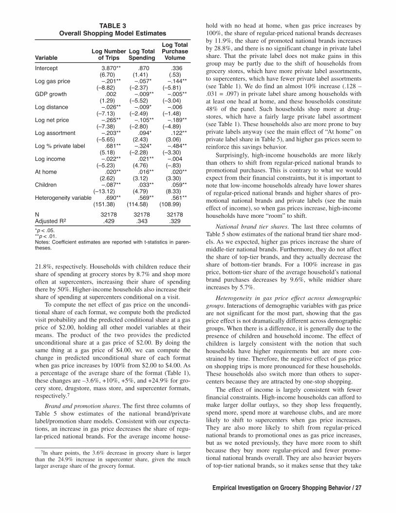
Brand and promotion shares. The first three columns ofTable 5 show estimates of the national brand/privatelabel/promotion share models. Consistent with our expecta-tions, an increase in gas price decreases the share of regu-lar-priced national brands. For the average income house-


hold with no head at home, when gas price increases by100%, the share of regular-priced national brands decreasesby 11.9%, the share of promoted national brands increasesby 28.8%, and there is no significant change in private labelshare. That the private label does not make gains in thisgroup may be partly due to the shift of households fromgrocery stores, which have more private label assortments,to supercenters, which have fewer private label assortments(see Table 1). We do find an almost 10% increase (.128 –.031 = .097) in private label share among households withat least one head at home, and these households constitute48% of the panel. Such households shop more at drug-stores, which have a fairly large private label assortment(see Table 1). These households also are more prone to buyprivate labels anyway (see the main effect of “At home” onprivate label share in Table 5), and higher gas prices seem toreinforce this savings behavior.

Surprisingly, high-income households are more likelythan others to shift from regular-priced national brands topromotional purchases. This is contrary to what we wouldexpect from their financial constraints, but it is important tonote that low-income households already have lower sharesof regular-priced national brands and higher shares of pro-motional national brands and private labels (see the maineffect of income), so when gas prices increase, high-incomehouseholds have more “room” to shift.

National brand tier shares. The last three columns ofTable 5 show estimates of the national brand tier share mod-els. As we expected, higher gas prices increase the share ofmiddle-tier national brands. Furthermore, they do not affectthe share of top-tier brands, and they actually decrease theshare of bottom-tier brands. For a 100% increase in gasprice, bottom-tier share of the average household’s nationalbrand purchases decreases by 9.6%, while midtier shareincreases by 5.7%.

Heterogeneity in gas price effect across demographicgroups. Interactions of demographic variables with gas priceare not significant for the most part, showing that the gasprice effect is not dramatically different across demographicgroups. When there is a difference, it is generally due to thepresence of children and household income. The effect ofchildren is largely consistent with the notion that suchhouseholds have higher requirements but are more con-strained by time. Therefore, the negative effect of gas priceon shopping trips is more pronounced for these households.These households also switch more than others to super-centers because they are attracted by one-stop shopping.

The effect of income is largely consistent with fewerfinancial constraints. High-income households can afford tomake larger dollar outlays, so they shop less frequently,spend more, spend more at warehouse clubs, and are morelikely to shift to supercenters when gas price increases.They are also more likely to shift from regular-pricednational brands to promotional ones as gas price increases,but as we noted previously, they have more room to shiftbecause they buy more regular-priced and fewer promo-tional national brands overall. They are also heavier buyersof top-tier national brands, so it makes sense that they take

7In share points, the 3.6% decrease in grocery share is largerthan the 24.9% increase in supercenter share, given the muchlarger average share of the grocery format.

TABlE 3Overall Shopping Model Estimates

log Totallog Number log Total Purchase

Variable of Trips Spending Volume

Intercept 3.870** .870 .336(6.70) (1.41) (.53)

Log gas price –.201** –.057* –.144**(–8.82) (–2.37) (–5.81)

GDP growth .002 –.009** –.005**(1.29) (–5.52) (–3.04)

Log distance –.026** –.009* –.006(–7.13) (–2.49) (–1.48)

Log net price –.265** –.105** –.189**(–7.38) (–2.80) (–4.89)

Log assortment –.203** .094* .122**(–5.65) (2.43) (3.06)

Log % private label .681** –.324* –.484**(5.18) (–2.28) (–3.30)

Log income –.022** .021** –.004(–5.23) (4.76) (–.83)

At home .020** .016** .020**(2.62) (3.12) (3.30)

Children –.087** .033** .059**(–13.12) (4.79) (8.33)

Heterogeneity variable .690** .569** .561**(151.38) (114.58) (108.99)

N 32178 32178 32178Adjusted R2 .429 .343 .329

*p < .05.**p < .01.Notes: Coefficient estimates are reported with t-statistics in paren-theses.

28/ Journal of M

arketing, March 2011

TABlE 4Format Share Model

Grocery Store Drugstore Mass Store Supercenter Club

Variable log Share Probit log Share Probit log Share Probit log Share Probit log Share

Intercept –.192*** 1.432*** –.985*** 1.334*** –1.059*** .918*** –.973*** 1.170*** –.185**

(–32.87) (15.75) (–11.04) (43.15) (–35.33) (20.53) (–13.59) (14.23) (–2.43)Log gas price (GPrice) –.010 –.173** .382*** –.209*** .218*** .178** .178 –.000 .003

(–.36) (–2.34) (5.19) (–2.87) (2.71) (2.04) (1.17) (0) (.04)GDP growth .005*** –.005 –.010** .004 –.008** –.014*** –.026*** .008 –.015***

(3.38) (–1.18) (–2.29) (1.04) (–1.96) (–2.87) (–3.09) (1.50) (–2.73)Log relative distance –.006 –.021** .060*** –.088*** .051*** –.194*** –.107*** –.077*** .023

(–.90) (–2.42) (6.25) (–9.06) (4.62) (–20.64) (–6.48) (–6.57) (1.63)Log relative net price –1.023*** –.313 –.554** –.352* 1.214*** .512** 1.628*** –.133 .206

(–4.77) (–1.51) (–2.53) (–1.92) (5.80) (2.47) (5.17) (–1.17) (1.50)Log relative assortment .129*** –.028 .414*** .048 –.171** .004 .017 .055 .495***(3.36) (–.41) (5.85) (.75) (–2.30) (.07) (.13) (.82) (7.18)Log relative % private label –2.169*** –.421 –1.931*** .318 1.029*** .032 .428 .353 –.507*

(–13.02) (–1.49) (–6.81) (1.23) (3.51) (.14) (.90) (1.44) (–1.87)Log income –.003 –.140*** –.069*** –.024* –.038*** .038*** –.050** .254*** .176***

(–.55) (–11.23) (–5.39) (–1.95) (–2.86) (2.64) (–2.00) (16.69) (9.91)At home –.037*** .018 .047*** .006 –.087*** –.014 –.047 .073*** .000

(–5.98) (1.14) (2.63) (.36) (–5.06) (–.78) (–1.49) (4.00) (.02)Kids .033*** –.096*** –.173*** .052*** .009 .065*** .058* –.099*** .009

(4.75) (–5.47) (–8.23) (2.98) (.49) (3.24) (1.73) (–5.00) (.45)Log GPrice × log income –.000 –.159** .014 –.001 .252**

(–.01) (–2.34) (.19) (–.01) (1.85)Log GPrice × at home –.044 .057 –.021 .041 .133

(–1.27) (.64) (–.22) (.39) (.77)Log GPrice × kids –.087** .022 .100 .260** .501***

(–2.33) (.23) (.96) (2.39) (2.75)Log heterogeneity variable .164*** .419*** .286*** .349*** .261*** .326*** .198*** .403*** .141***

(13.62) (56.71) (32.17) (59.68) (36.69) (45.88) (18.29) (64.50) (19.61)

N 31,286 32,178 16,274 32,178 17,725 32,178 6287 32,178 8657Adjusted R2 .209 .306 .174 .264 .146 .249 .148 .404 .158

*p < .10.**p < .05.***p < .01.Notes: All shares are shares of total purchase volume. Coefficient estimates are reported with t-statistics in parentheses.

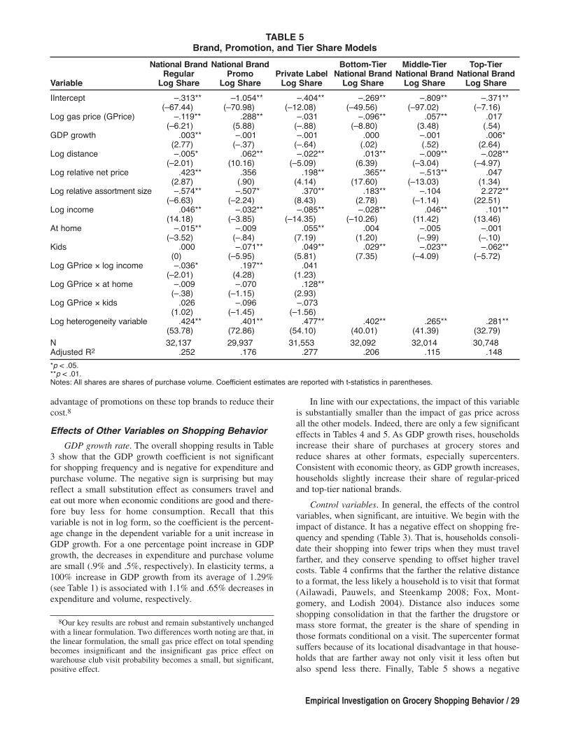
advantage of promotions on these top brands to reduce theircost.8

Effects of Other Variables on Shopping Behavior

GDP growth rate. The overall shopping results in Table3 show that the GDP growth coefficient is not significantfor shopping frequency and is negative for expenditure andpurchase volume. The negative sign is surprising but mayreflect a small substitution effect as consumers travel andeat out more when economic conditions are good and there-fore buy less for home consumption. Recall that thisvariable is not in log form, so the coefficient is the percent-age change in the dependent variable for a unit increase inGDP growth. For a one percentage point increase in GDPgrowth, the decreases in expenditure and purchase volumeare small (.9% and .5%, respectively). In elasticity terms, a100% increase in GDP growth from its average of 1.29%(see Table 1) is associated with 1.1% and .65% decreases inexpenditure and volume, respectively.


In line with our expectations, the impact of this variableis substantially smaller than the impact of gas price acrossall the other models. Indeed, there are only a few significanteffects in Tables 4 and 5. As GDP growth rises, householdsincrease their share of purchases at grocery stores andreduce shares at other formats, especially supercenters.Consistent with economic theory, as GDP growth increases,households slightly increase their share of regular-pricedand top-tier national brands.

Control variables. In general, the effects of the controlvariables, when significant, are intuitive. We begin with theimpact of distance. It has a negative effect on shopping fre-quency and spending (Table 3). That is, households consoli-date their shopping into fewer trips when they must travelfarther, and they conserve spending to offset higher travelcosts. Table 4 confirms that the farther the relative distanceto a format, the less likely a household is to visit that format(Ailawadi, Pauwels, and Steenkamp 2008; Fox, Mont-gomery, and Lodish 2004). Distance also induces someshopping consolidation in that the farther the drugstore ormass store format, the greater is the share of spending inthose formats conditional on a visit. The supercenter formatsuffers because of its locational disadvantage in that house-holds that are farther away not only visit it less often butalso spend less there. Finally, Table 5 shows a negative

8Our key results are robust and remain substantively unchangedwith a linear formulation. Two differences worth noting are that, inthe linear formulation, the small gas price effect on total spendingbecomes insignificant and the insignificant gas price effect onwarehouse club visit probability becomes a small, but significant,positive effect.

TABlE 5Brand, Promotion, and Tier Share Models

National Brand National Brand Bottom-Tier Middle-Tier Top-TierRegular Promo Private label National Brand National Brand National Brand

Variable log Share log Share log Share log Share log Share log Share

IIntercept –.313** –1.054** –.404** –.269** –.809** –.371**(–67.44) (–70.98) (–12.08) (–49.56) (–97.02) (–7.16)

Log gas price (GPrice) –.119** .288** –.031 –.096** .057** .017(–6.21) (5.88) (–.88) (–8.80) (3.48) (.54)

GDP growth .003** –.001 –.001 .000 –.001 .006*(2.77) (–.37) (–.64) (.02) (.52) (2.64)

Log distance –.005* .062** –.022** .013** –.009** –.028**(–2.01) (10.16) (–5.09) (6.39) (–3.04) (–4.97)

Log relative net price .423** .356 .198** .365** –.513** .047(2.87) (.90) (4.14) (17.60) (–13.03) (1.34)

Log relative assortment size –.574** –.507* .370** .183** –.104 2.272**(–6.63) (–2.24) (8.43) (2.78) (–1.14) (22.51)

Log income .046** –.032** –.085** –.028** .046** .101**(14.18) (–3.85) (–14.35) (–10.26) (11.42) (13.46)

At home –.015** –.009 .055** .004 –.005 –.001(–3.52) (–.84) (7.19) (1.20) (–.99) (–.10)

Kids .000 –.071** .049** .029** –.023** –.062**(0) (–5.95) (5.81) (7.35) (–4.09) (–5.72)

Log GPrice × log income –.036* .197** .041(–2.01) (4.28) (1.23)

Log GPrice × at home –.009 –.070 .128**(–.38) (–1.15) (2.93)

Log GPrice × kids .026 –.096 –.073(1.02) (–1.45) (–1.56)

Log heterogeneity variable .424** .401** .477** .402** .265** .281**(53.78) (72.86) (54.10) (40.01) (41.39) (32.79)

N 32,137 29,937 31,553 32,092 32,014 30,748Adjusted R2 .252 .176 .277 .206 .115 .148

*p < .05.**p < .01.Notes: All shares are shares of purchase volume. Coefficient estimates are reported with t-statistics in parentheses.

effect of distance on private label share and a positive effecton promotional national brand share. Consumers alsoreduce mid- and top-tier brand shares and increase bottom-tier brand shares when they must travel farther to shop. Thismay be to offset driving cost, but it could also be becausethe retail formats that are farthest away (warehouse clubs)have a lower-than-average top-tier assortment and a higher-than-average bottom-tier assortment (Table 1).

The effect of net price is not always negative. Net pricehas the expected negative effect on shopping trips, purchasevolume, and expenditure. With a couple of exceptions, italso has the expected negative effect in the format sharemodels, though it is not always significant. This is consis-tent with the mixed effect of price in prior research (e.g.,Fox, Montgomery, and Lodish 2004). The positive effect forregular national brand and private label shares is consistentwith previous findings that the price differential betweenprivate labels and national brands may be too big and thatprivate labels can benefit from reducing the differential(Ailawadi, Pauwels, and Steenkamp 2008; Hoch andBanerji 1993).

Finally, the impact of assortment is noteworthy. It isnegative for shopping frequency; we presume that consumersneed fewer shopping trips to find what they need when assort-ment is large. Both spending and purchase volume increasewith the variety of choices offered by a bigger assortment.In addition, we find that the more the private label is empha-sized in the total assortment, the more frequently house-holds shop, and the lower is their purchase volume andspending. Consistent with prior research (e.g., Ailawadi,Pauwels, and Steenkamp 2008), this suggests that empha-sizing private labels too much is not good for retailers.

As we expected, in general the relative size of a for-mat’s assortment increases its share, with the exceptionbeing the mass store format. As grocery stores and drug-stores increase their emphasis on private labels, householdslower their visits and share of spending there, but the oppo-site is true for mass stores. This is consistent with differentexpectations and objectives in shopping trips made to dif-ferent formats (Fox and Sethuraman 2006). Consumerswant variety at the local grocery store and drugstores andlower-priced private labels when they visit a mass store.Table 5 shows that assortment size has the expected positiveeffect for bottom- and top-tier national brands and for pri-vate labels, but surprisingly, it has a negative effect for regu-lar and promoted national brand share. The latter is consis-tent with prior findings that sales actually improve whenretailers prune assortment strategically (Broniarczyk,Hoyer, and McAlister 1998).

Demographic variables. The main effects of demograph-ics on shopping behavior are largely in line with intuition.Table 3 shows that income has a negative effect on the num-ber of shopping trips and a positive effect on spending. Botheffects make sense because the financial constraints of low-income households encourage them to search more andtherefore make more trips; according to basic economictheory, high-income households can afford to spend more.Table 4 shows that high-income households make fewervisits to drugstores and mass stores and also have lower


shares in these formats conditional on a visit. They alsovisit supercenters and warehouse clubs more often and havehigher warehouse club share conditional on a visit, perhapsbecause they can afford the budget outlay required for bulkshopping. Finally, Table 5 shows that, consistent with basiceconomic theory, high-income households have highershares of regular-priced national brands and middle- andtop-tier national brands and lower shares of promotionaland bottom-tier national brands and private labels.

Households with at least one nonworking householdhead make slightly more trips, consistent with fewer timeconstraints, and their volume and spending are also slightlygreater (Table 3). They spend less at grocery and mass storesand more at drugstores (Table 4). This may have less to dowith their time constraints (or lack thereof) and more to dowith the probability that they are older and/or retired, aprime target market for drugstores. They buy fewer regular-priced national brands, but surprisingly, they buy more pri-vate labels, not more promotional national brands, despitetheir fewer time constraints. This finding may be related totheir preference for drugstores, which carry a higher per-centage of private label products than supercenters andwarehouse clubs (Table 1).

In general, the impact of children is intuitive. House-holds with children make fewer shopping trips, presumablybecause of time constraints, but their total expenditure andpurchase volume are higher because of the greater needs oflarge families. They visit and spend less at drugstores,which is consistent with the older, female target market ofdrugstore chains. In contrast, they spend more at grocerystores, mass stores, and supercenter formats. They are timeconstrained, and they need to save money on their largeshopping baskets, so they prefer formats that balance con-venience (grocery store) with affordability (mass store andsupercenter). Also in line with intuition, time-constrainedhouseholds with children buy more private labels and fewernational brands on promotion.

DiscussionMacroeconomic conditions have major effects on consumerbehavior and, therefore, on firm performance. This researchprovides a comprehensive, disaggregate analysis of howand how much consumers change their grocery shoppingbehavior in response to gas price, a macroeconomicvariable that is increasing in importance. In quantifying theeffect of gas price, we control for general macroeconomicconditions as reflected in the GDP growth rate. On the onehand, our work complements aggregate research on theimpact of macro factors, and on the other hand, it builds onthe large body of research on consumer grocery shoppingbehavior, which examines a host of variables, such as price,promotions, assortment, and competitive factors, but in gen-eral does not incorporate macroeconomic factors.

Gas Price Effect

We summarize the estimated average magnitude of the gasprice effect on each component of shopping behavior inFigure 3. For easy interpretation, the magnitudes are interms of elasticities, that is, the percentage change in a com-

ponent of shopping behavior for the average household,attributable to a 100% increase in gas price (e.g., from$2.00 per gallon to $4.00 per gallon). We summarize theeffect of gas price as follows: Households consume less andconsolidate their shopping as rising gas prices take a biggerbite out of their wallet, but they preserve their preferencefor high-quality brands, searching for them on promotion tosave money. Next, we highlight the aspects of these resultsthat are either surprising or contrary to conventional wis-dom and discuss their implications.

We found that an increase in gas prices reduces shop-ping frequency and purchase volume, and though this maynot seem surprising, it is important for at least two reasons.First, although prior research has established a strong effectof macroeconomic factors, such as recessions and lowerconsumer confidence, on sales of durable goods, consumerpackaged goods products are considered more habitual andnecessary, less conducive to purchase postponement, and,therefore, less vulnerable (Deleersnyder et al. 2004; Katona1975). Second, evidence shows that consumers travel lessand eat at home more as gas prices rise, so there is a posi-tive substitution effect that should increase food purchases.Indeed, Gicheva, Hastings, and Villas-Boas (2010) report apositive effect of gas price on expenditure in four food cate-gories. Despite these phenomena, we document a substan-tial reduction especially in overall purchase volume whenwe include a comprehensive array of grocery products andcontrol for other variables. Apart from the general decreasein purchase volume, which hurts both manufacturers andretailers, manufacturers of impulse products may be espe-cially hurt by lower shopping frequency as impulse pur-chase opportunities decrease. In addition, consumers willstockpile, so manufacturers and retailers should offer fre-


quent promotions to generate shopping trips and increasethe opportunities for consumers to select their offering.

In general, the impact of gas prices on where consumersshop is intuitive: They consolidate their shopping. Drivenlargely by households with children, supercenters, the quin-tessential one-stop shopping format, benefit at the expenseof traditional grocery stores. Although consumers visitdrugstores and mass stores less, they buy a larger share oftheir requirements there when they do visit, and the netimpact is slightly positive. Manufacturers need to considerthe shift in consumer choice as they negotiate prices andtrade deals with the different formats. They may need tooffer more promotional funds to the traditional formats tokeep them competitive while engaging the supercenterchannel with different, possibly larger-size stockkeepingunits that higher-income and larger households are willingto buy.

Consistent with economic theory, higher gas pricesmake households shift away from regular- to promotional-priced national brands. The shift toward private labels ismuch smaller. Indeed, there is no significant impact on pri-vate label share except among households with one head athome. This is a surprising finding given the attention in thebusiness press to private label growth, and its implicationsare important. Retailers should realize that continuing toemphasize private labels at the expense of national brands,unless it is accompanied by credible quality improvementsand strong marketing and differentiation (Ailawadi,Pauwels, and Steenkamp 2008), may not increase shareeven in tight times. Promotions are an effective retentiontool as gas prices increase, so balancing a robust privatelabel with attractive promotions on national brands is morelikely to be effective. Manufacturers should also realize that

Notes: Percentage changes in shares are from the average share of each option. Therefore, in share points, the 3.6% decrease in groceryshare is larger than the 24.9% increase in supercenter share, given the much larger average share of the grocery format.

Format Shares•3.6% decrease in grocery format share, driven by householdswith children

•10% increase in drugstore format share, despite lower visitprobability

•5% increase in mass format share, despite lower visit probability•24.9% increase in supercenter format share, driven especiallyby households with children

•No significant change in warehouse club format share

Brand/Promotion Shares•12% decrease in regular-priced national brand share•29% increase in promotional national brand share •3% increase in private label share, driven by households withone or more head at home

National Brand Tier Shares•10% decrease in share of bottom-tier brands•6% increase in share of midtier brands•No significant change in share of top-tier brands

100% increase ingas price from$2.00 to $4.00

6% decrease in monthly

expenditure

14% decrease inmonthly purchase

volume

20% decrease inmonthly shopping

trips

FIGURE 3Summary of Average Gas Price Effect

hunkering down in tough times by cutting promotions andallowing prices to rise will lead to share losses (see Deleer-snyder et al. 2004). Furthermore, given prior research on theasymmetry of consumer shifts (Lamey et al. 2007), con-sumers lost during tough times may not return when finan-cial constraints are eased.

Equally important is our finding that higher gas pricesdo not hurt the share of top-tier brands among consumerswho continue to purchase national brands. Rather, it is theshare of bottom-tier brands that drops, while midtier brandsgain. This finding is contrary to the conventional wisdomthat top-tier brands suffer when times are tough but is con-sistent with research on context effects; private labels aremuch more likely to take share away from bottom-tierbrands than from top-tier ones. Thus, manufacturers shouldtread carefully in introducing lower-priced extensions oftheir high-equity brands. Unless they can significantly cutcosts and preserve margins at the substantially lower priceneeded to combat private labels, they may find that thelower-tier introductions are not effective in retaining cus-tomers and may end up hurting their overall brand equity. Itwould be worthwhile to monitor the performance of “basic”versions of national brands that companies such as Procter& Gamble have begun introducing (Bryon 2009).

In summary, the most direct way consumers can offsethigher gas prices is by using less gas, but the economics lit-erature has convincingly shown that gasoline demand isfairly inelastic. Our results show that travel cost plays a rolein consumer shopping shifts, but it is far from the sole deter-minant. On the one hand, shopping frequency decreasessubstantially as gas prices increase. Distance is an impor-tant control variable in our models and shows the expectednegative sign. Furthermore, the one-stop shopping super-center format increases share as gas prices rise. On the otherhand, supercenters are generally farther away, and con-sumers buy more on promotion as gas prices increase,despite the need to search at different times and in differentstores. In addition, sensitivity to distance does not becomestronger with gas price increases, except in the shoppingtrip model. Overall, therefore, our results underscore theimportance of considering not just monetary cost but alsothe full spectrum of other economic costs and, to a lesserextent, the psychosocial aspects of shopping in understand-ing consumer shopping response to macroeconomic factorssuch as gas price.

Limitations

We note some limitations of our work that we hoperesearchers can address. First, we estimate the impact of gasprice on each component of shopping behavior separately.However, it is likely that consumers’ shopping decisions areinterdependent or follow a hierarchical structure (e.g., theyfirst decide on their budget and where to shop and thendecide what to buy). We leave this to further research to testmore integrated models.

Second, although we allow for heterogeneity in the gasprice effect across key demographic groups, there may beheterogeneity in response among consumers that thesedemographic variables do not capture. For example, con-sumers with different psychographic and shopping profiles


may react differently. Generating such profiles and studyingdifferences in their response are fruitful directions for addi-tional research.

Third, although we control for economic conditionswith the well-accepted GDP growth variable and find simi-lar results to the Conference Board Composite Index ofCoincident Indicators, other macroeconomic variables mayaffect shopping behavior and should be examined, espe-cially when the data span longer periods. Similarly, weaccount for key marketing-mix variables, but other retailfactors, such as service and convenience (Ailawadi andKeller 2004; Berry, Seiders, and Grewal 2002; Gauri,Trivedi, and Grewal 2008), influence consumers’ formatand store choice. To the extent that these factors are stable,we control for them through the heterogeneity variable.However, further research should examine whether theinfluence of these factors changes with the macroeconomicenvironment.

Conclusion

The significant effect of gas price we document hereinmakes it important to incorporate this factor explicitly intoconsumer shopping behavior models when it exhibits sub-stantial variance. We also contrast the effects of gas priceand general economic health on grocery shopping and findthat the former is much stronger. Although we examine theshort-term impact, it is important to understand whetherthese changes persist over the long run and whether theyreverse when gas price goes down again. Furthermore, it isimportant to understand the extent to which shoppingbehavior changes are driven by psychological factors ratherthan the direct budgetary constraints that higher gas pricesimpose. Gas prices and general economic conditions arelikely to have very different effects on consumer sentimentand attitudes, which in turn affect consumers’ psychologicalwillingness to buy. Finally, we show that gas price is justone important macroeconomic variable outside the controlof managers that influences consumer shopping. Othermacroeconomic variables, such as home values and taxrates, might also affect consumers’ willingness and/or abil-ity to buy. We hope that our work stimulates furtherresearch in this important domain.

AppendixVariable Definitions

We aggregate all variables from the category to the formatand market level using household-specific category and for-mat shares in the initialization period as weights.9 We usethe first two months as the initialization period.

Variables for Format Share Models

Distancehj. Distance to retail format j for household h iscalculated as

9The exception is net price of a category, which we aggregate upfrom stockkeeping unit and brand levels using market shares in theinitialization period as weights.

where disthjn is the distance from the closest store of retailern in format j to household h and tshjnt0 is the share ofretailer n in retail format j for household h in the initializa-tion period.

RelDisthj. Distance to format j for household h relativeto weighted average distance to all formats is calculated as

where tshjt0 is household h’s share of format j in the initializa-tion period.

NPricehjt. Net price is calculated as

where Npricejtc is net price of category c in format j inmonth t and csht0c is share of total spending by household hin the initialization period on category c.

RelNPricehjt. Net price of format j in month t for house-hold h, relative to weighted average net price of all formats,is calculated as

AssrtSizehjt. Assortment size of format j for household hin month t is calculated as

where AssrtSizejtc is the number of distinct stockkeeping unitsof category c in the quarter of month t in retail format j.

RelAssrtSizehjt. Assortment size of format j for house-hold h relative to weighted average assortment size of allformats is calculated as

PctPLhjt. Percentage private label in assortment of for-mat j for household h in quarter of month t is calculated as

Distance

Distance

hj

hj hjtj

ts 01

5

=∑

,

NPrice

NPricejtc

t cc

C

ht ccs01

0

=∑ ,

NPrice

NPrice

hjt

hjt hjtj

ts 01

5

=∑

.

AssrtSize csjtc

c

C

ht c

=∑

1

0 ,

AssrtSize

AssrtSize ts

hjt

hjt hjt

j

0

1

5

=∑

.

d tshjn hjnt

n

N

ist 0

1=∑ ,

PLPct csjtcc

C

ht c=

∑1

0 ,


where PLPctjtc is the percentage of the total assortment thatis private label in category c of format j in the uarter ofmonth t.

RelPctPLhjt. Percentage private label in assortment sizeof format j for household h relative to weighted averagepercentage private label in all formats is calculated as

Variables for Brand/Promotion Share Models

Distanceh. Average distance to stores for household h iscalculated as

where Distancehj is as defined previously and fshjt0 is theshare of total trips to retail format j by household h in theinitialization period.

NPricehkt. Net price is calculated as

where NPricekct is net price of brand type k in category c inmonth t and csht0c is as defined previously. Note that k = 1is national brands and k = 2 is private label.

RelNPricehkt. Relative net price is calculated as

where tshkt0 is household h’s share of brand type k in theinitialization period.

AssrtSizehkt. Assortment size of brand type k for house-hold h in month t is calculated as

where AssrtSizektc is the number of distinct stockkeepingunits of brand type k in category c in the quarter of month t.

RelAssrtSizehkt. Assortment size of brand type k forhousehold h relative to weighted average assortment size ofboth brand types is calculated as

PLPct

PLPct

hjt

hjt hjtj

ts 01

5

=∑

.

Distancehj

n

N

hjtfs=

∑1

0 ,

NPrice

NPricekct

ctc

C

ht ccs01

0=

∑ ,

NPrice

NPrice

hkt

hkt hktk

ts 01

2

=∑

,

AssrtSizektcc

C

ht ccs=

∑1

0 ,

AssrtSize

AssrtSize

hkt

hkt hktk

ts 01

2

=∑

.

Variables for National Brand Tier Share Models

These are calculated the same as previously, except that k =1, 2, and 3, respectively, for bottom-, mid-, and top-tiernational brands.

Variables for Overall Shopping Models

Distanceh. This is calculated as defined previously.

NPriceht, AssrtSizeht, and PctPLht. These are calculatedas follows:

NPrice

AssrtSize

hjtj

hjt

hjtj

hjt

ts

ts an

=

=

∑

∑1

5

0

1

5

0

,

, dd


where NPricehjt, AssrtSizehjt, PctPLhjt, and tshjt0 are as definedin the format share models.

Purchase Volumeht. Total purchase volume by householdh in month t is calculated as

where qhtc is total equivalent units of category c purchasedby household h in month t and NPricet0c is net price of cate-gory c in the initialization period.

PctPL tshjt

j

hjt

=∑

1

5

0 ,

q N icehtc

c

C

t c

=∑

1

0Pr ,

Demand: A SUR Approach,” Energy Economics, 30 (5),2105–22.

Bucklin, Randolph E., Sunil Gupta, and S. Han (1995), “A Brand’sEye View of Response Segmentation in Consumer BrandChoice Behavior,” Journal of Marketing Research, 32 (Febru-ary), 66–74.

Bryon, Ellen (2009), “Tide Turns ‘Basic’ for P&G in Slump,”(August 6), (accessed December 15, 2010), [available at http://online.wsj.com/article/SB124946926161107433.html].

Bureau of Labor Statistics (2007), “Consumer Expenditure Sur-vey,” (accessed November 4, 2010), [available at http://www.bls.gov/cex/csxstnd.htm#2007].

Chandon, Pierre, Brian Wansink, and Gilles Laurent (2000), “ABenefit Congruency Framework of Sales Promotion Effective-ness,” Journal of Marketing, 64 (October), 65–81.

Chintagunta, Pradeep K., Vrinda Kadiyali, and Naufel J. Vilcassim(2006), “Endogeneity and Simultaneity in Competitive Pricingand Advertising: A Logit Demand Analysis,” Journal of Busi-ness, 79 (6), 2761–87.

Deleersnyder, Barbara, Marnik G. Dekimpe, Miklos Sarvary, andPhilip M. Parker (2004), “Weathering Tight Economic Times:The Sales Evolution of Consumer Durables Over the BusinessCycle,” Quantitative Marketing & Economics, 2 (4), 347–83.

———, ———, Jan-Benedict E.M. Steenkamp, and Peter S.H.Leeflang (2009), “The Role of National Culture in Advertis-ing’s Sensitivity to Business Cycles: An Investigation AcrossContinents,” Journal of Marketing Research, 46 (October),623–36.

Du, Rex Y. and Wagner A. Kamakura (2008), “Where Did All ThatMoney Go? Understanding How Consumers Allocate TheirConsumption Budget,” Journal of Marketing, 72 (November),109–131.

Fox, Edward J., Alan L. Montgomery, and Leonard M. Lodish(2004), “Consumer Shopping and Spending Across Retail For-mats,” Journal of Business, 77 (2), S25–S60.

——— and Raj Sethuraman (2006), “Retail Competition,” inRetailing in the 21st Century: Current and Emerging Trends,Manfred Krafft and Murali K. Mantrala, eds. Berlin: Springer-Verlag, 193–210.

Frankenberger, Kristina and Roger Graham (2003), “Should FirmsIncrease Advertising Expenditures During Recessions?” ReportNo. 03-115, Marketing Science Institute.

Gauri, Dinesh K., K. Sudhir, and Debabrata Talukdar (2008), “TheTemporal and Spatial Dimensions of Price Search: Insightsfrom Matching Household Survey and Purchase Data,” Journalof Marketing Research, 45 (April), 226–40.

REFERENCESAilawadi, Kusum L. and Bari Harlam (2004), “An Empirical

Analysis of the Determinants of Retail Margins: The Role ofStore-Brand Share,” Journal of Marketing, 68 (January),147–65.

——— and ——— (2009), “Retailer Promotion Pass-Through: AMeasure, Its Magnitude, and Its Determinants,” Marketing Sci-ence, 28 (4), 782–91.

——— and Kevin Keller (2004), “Understanding Retail Branding:Conceptual Insights and Research Priorities,” Journal ofRetailing, 80 (4), 331–42.

———, Scott A. Neslin, and Karen Gedenk (2001), “Pursuing theValue-Conscious Consumer: Store Brands Versus NationalBrand Promotions,” Journal of Marketing, 65 (January),71–89.

———, Koen Pauwels, and Jan-Benedict E.M. Steenkamp (2008),“Private-Label Use and Store Loyalty,” Journal of Marketing,72 (November), 19–30.

Allenby, Gregory, L. Jen, and Robert Leone (1996), “EconomicTrends and Being Trendy: The Influence of Consumer Confi-dence on Retail Fashion Sales,” Journal of Business & Eco-nomic Statistics, 14 (1), 103–111.

Bell, David R., Teck-Hua Ho, and Christopher S. Tang (1998),“Determining Where to Shop: Fixed and Variable Costs ofShopping,” Journal of Marketing Research, 35 (August),352–69.

Berry, Leonard L., Kathleen Seiders, and Dhruv Grewal (2002),“Understanding Service Convenience,” Journal of Marketing,66 (July), 1–17.

Bhatnagar, Amit and Brian T. Ratchford (2004), “A Model ofRetail Format Competition for Non-Durable Goods,” Interna-tional Journal of Research in Marketing, 21 (1), 39–59.

Blattberg, Robert, Thomas Buesing, Peter Peacock, and SubrataSen (1978), “Identifying Deal Prone Segment,” Journal ofMarketing Research, 15 (August), 369–77.

——— and Kenneth J. Wisniewski (1989), “Price-Induced Pat-terns of Competition,” Marketing Science, 8 (4), 291–309.

Briesch, Richard A., Pradeep K. Chintagunta, and Edward J. Fox(2009), “How Does Assortment Affect Grocery Store Choice?”Journal of Marketing Research, 46 (April), 176–89.

Broniarczyk, Susan M., Wayne D. Hoyer, and Leigh McAlister(1998), “Consumers’ Perceptions of the Assortment Offered ina Grocery Category: The Impact of Item Reduction,” Journalof Marketing Research, 35 (May), 166–76.

Brons, Martjin, Peter Nijkamp, Eric Pels, and Piet Rietveld(2008), “A Meta-Analysis of the Price Elasticity of Gasoline

———, Minakshi Trivedi, and Dhruv Grewal (2008), “Under-standing the Determinants of Retail Strategy,” Journal ofRetailing, 84 (3), 256–67.

Geyskens, Inga, Katrijn Gielens, and Marnik Dekimpe (2002),“The Market Valuation of Internet Channel Additions,” Journalof Marketing, 66 (April), 102–119.

———, ———, and Els Gijsbrecht (2010), “Proliferating Private-Label Portfolios: How Introducing Economy and Premium Pri-vate Labels Influences Brand Choice,” Journal of MarketingResearch, 47 (October), 791–807.

Gicheva, Dora, Justine Hastings, and Sofia Villas-Boas (2010),“Revisiting the Income Effect: Gasoline Prices and GroceryPurchases,” American Economic Review, 100 (2), 480–84.

Greening, Lorna A., Han Tarn Jeng, John P. Formby, and David C.Cheng (1995), “Use of Region, Life-Cycle and Role Variablesin the Short-Run Estimation of the Demand for Gasoline andMiles Traveled,” Applied Economics, 27 (7), 643–56.

Grewal, Dhruv, Michael Levy, and V. Kumar (2009), “CustomerExperience Management in Retailing: An Organizing Frame-work,” Journal of Retailing, 85 (1), 1–14.

Griffith, Rachel, Ephraim Leibtag, Andrew Leicester, and AvivNevo (2009), “Consumer Shopping Behavior: How Much DoConsumers Save?” Journal of Economic Perspectives, 23 (2),99–120.

Hamilton, James D (2008), “Oil and the Macroeconomy,” in NewPalgrave Dictionary of Economics, 2d ed., Steven Durlauf andLawrence Blume, eds. New York: Palgrave McMillan.

Hoch, Stephen J. and Shumeet Banerji (1993), “When Do PrivateLabels Succeed?” Sloan Management Review, 34 (4), 57–67.

Jacobe, Dennis (2006), “High Gas Prices Causing ConsumerSpending Cuts,” Gallup News Service, (May 24), (accessedNovember 22, 2010), [available at http://www.gallup.com/poll/22918/high-gas-prices-causing-consumer-spending-cuts.aspx].

Katona, George (1975), Psychological Economics. New York:Elsevier Scientific Publishing.

Kumar, Nirmalya and Jan-Benedict E.M. Steenkamp (2007), Pri-vate Label Strategy: How to Meet the Store Brand Challenge.Boston: Harvard Business School Press.

Kumar, V., Robert P. Leone, and John N. Gaskins (1995), “Aggre-gate and Disaggregate Sector Forecasting Using ConsumerConfidence Measures,” International Journal of Forecasting,11 (3), 361–77.

Lamey, Lien, Barbara Deleersnyder, Marnik G. Dekimpe, and Jan-Benedict E.M. Steenkamp (2007), “How Business Cycles Con-tribute to Private-Label Success: Evidence from the UnitedStates and Europe,” Journal of Marketing, 71 (January), 1–15.


Luchs, Ryan J., Jeffrey Inman, and Venkatesh Shankar (2007),“Channel Blurring: A Study of Cross-Retail Format ShoppingAmong U.S. Households,” working paper, Katz GraduateSchool of Business, University of Pittsburgh.

Marmorstein, Howard, Dhruv Grewal, and Raymond Fishe (1992),“The Value of Time Spent in Price-Comparison Shopping: Sur-vey and Experimental Evidence,” Journal of ConsumerResearch, 19 (1), 52–61.

Mouawad, Jad and Mireya Navarro (2008), “Teeth Gritted, DriversAdjust to $4 Gasoline,” The New York Times, (May 24),(accessed November 22, 2010), [available at http://www.nytimes.com/2008/05/24/business/24gas.html?_r=1&scp=1&sq=Teeth%20Gritted,%20Drivers%20Adjust%20to%20%244%20Gaso-line%20&st=cse].

Narasimhan, Chakravarthi, Scott A. Neslin, and Subrata Sen(1996), “Promotional Elasticities and Category Characteris-tics,” Journal of Marketing, 60 (April), 17–30.

Nevo, Aviv (2001), “Measuring Market Power in the Ready-to-EatCereal Industry,” Econometrica, 69 (2), 307–342.

Pauwels, Koen and Shuba Srinivasan (2004), “Who Benefits fromStore Brand Entry?” Marketing Science, 23 (3), 364–90.

Private Label Manufacturers Association (2009), “PLMA Year-book Documents Private Label Sales Surge of More Than105,” (accessed November 3, 2010), [available at http://www.plma.com/pressupdate/pressupdate.asp#ID39].

Putrevu, Sanjay and Brian T. Ratchford (1997), “A Model ofSearch Behavior with an Application to Grocery Shopping,”Journal of Retailing, 73 (4), 463–86.

Sethuraman, Raj (2000), “What Makes Consumers Pay More forNational Brands Than for Store Brands: Image or Quality?”Report No. 00-110. Marketing Science Institute.

———, V. Srinivasan, and Doyle Kim (1999), “Asymmetric andNeighborhood Cross-Price Effects: Some Empirical General-izations,” Marketing Science, 18 (1), 23–41.

Srinivasan, Raji, Arvind Rangaswamy, and Gary Lilien (2005),“Turning Adversity into Advantage: Does Proactive MarketingDuring a Recession Pay Off?” International Journal ofResearch in Marketing, 22 (2), 109–125.

Urbany, Joel E., Peter R. Dickson, and Rosemary Kalapurakal(1996), “Price Search in the Retail Grocery Market,” Journal ofMarketing, 60 (April), 91–104.

The Wall Street Journal (2008), “Income vs. Gas Prices, anUpdate,” (August 4), (accessed November 22, 2010), [availableat http://blogs.wsj.com/economics/2008/08/04/ income-vs-gas-prices-an-update/].

Wooldridge, Jeffrey M. (2002), Econometric Analysis of CrossSection and Panel Data. Cambridge, MA: MIT Press.

Copyright of Journal of Marketing is the property of American Marketing Association and its content may not

be copied or emailed to multiple sites or posted to a listserv without the copyright holder's express written

permission. However, users may print, download, or email articles for individual use.