Physics DepartmentYarmouk University 21163 Irbid Jordan

Phys. 441: Nuclear Physics 1

Chapter V: Scattering Chapter V: Scattering Theory Theory -- ApplicationApplication

Lecture 17

http://ctaps.yu.edu.jo/physics/Courses/Phys641/Lec5-1

© Dr. Nidal Ershaidat

This Chapter:1- Introduction - Importance of the scattering theory.2- Cross-Section.

3- Scattering by a Potential.

5- Scattering Stationary States.

6- Probability Currents.

7- Applications. Central PotentialReferences:1. Quantum Mechanics, Vol. 2 Chapter VIIIChapter VIII

C. Cohen-Tannoudji, B. Diu and F. Laloë2. Quantum Physics, Chapter 19

Stephen Gasiorowicz

4- The Optical Theorem.

Introduction

4

Scattering evokes a simple image:

“What is scattering?”

Separate objects which are far apart and moving towards each other collide after some time and then travel away from each other and eventually are far apart again. We don’t necessarily care about the details of the collision except insofar as we can predict from it where and how the objects will end up.This picture of scattering is the first one we physicists learn.

5

A beautiful example of the power of conservation laws

“In many cases the laws of conservation of momentum and energy alone can be used to obtain important results concerning the properties of various mechanical processes. It should be noted that these properties are independent of the particular type of interaction between the particles involved”L.D. Landau Mechanics (1976)

6

An incident beam of particles (1) strikes a target. Two devices (detectors) are placed in order to detect the reaction results.

General Scheme

Fig. 5-1

7

The final state can be composed of new entities. In nuclear physics the outgoing particle b and the Y are the result of a rearrangement of nucleons and the process is called “rearrangement collision”

Elastic and Inelastic Scattering

Another important case is when the final state is composed of the same particles as in the initial state. Here we call the process “elastic scattering”. Otherwise it is called “inelastic scattering”

8

Knowing the initial state of the reaction and measuring the final state gives an idea about the nature of the reaction.

Understanding the reaction

In quantum mechanics language the interaction potential of the process can be understood.

In general, a scattering experiment aims to verify a theoretical model about the reaction.

Importance of the scattering theory

10

Since Rutherford’s explanation of Geiger and Marsden results, physicists understood that more energetic particles than the ααααparticles were necessary to “probe” the nucleus.

Understanding Matter

In addition quantum mechanics is necessary in order to understand what happens when a nucleus is bombarded by such a projectile.

Collision or Scattering Theory is the frame used by Physicists for this purpose.

11

On the experimental level this led to build accelerators more and more capable of providing high energy particles (electrons, protons or alpha’s, heavy ions …………).

Accelerators

On the theoretical level this type of experiments led to major developments in quantum mechanics.

Accelerators

See Supplements 6

13

The first probes used for investigating the nuclear structure were high energy electrons.

Electron Scattering - Hofstadter

Hofstadter used the first SLAC (Stanford Linear accelerator) to investigate the charge distribution in atomic nuclei and afterwards the charge and magnetic moment distributions in the proton and neutron. The electron-scattering method was used to find the size and surface thickness parameters of nuclei.

Electron Scattering and the Structure of the Nucleus

See Supplements 7

15

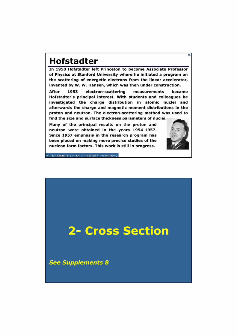
In 1950 Hofstadter left Princeton to become Associate Professor of Physics at Stanford University where he initiated a program on the scattering of energetic electrons from the linear accelerator, invented by W. W. Hansen, which was then under construction.

Hofstadter

After 1953 electron-scattering measurements became Hofstadter's principal interest. With students and colleagues heinvestigated the charge distribution in atomic nuclei and afterwards the charge and magnetic moment distributions in the proton and neutron. The electron-scattering method was used to find the size and surface thickness parameters of nuclei.

Many of the principal results on the proton and neutron were obtained in the years 1954-1957. Since 1957 emphasis in the research program has been placed on making more precise studies of the nucleon form factors. This work is still in progress.

2- Cross Section

See Supplements 8

Physics DepartmentYarmouk University 21163 Irbid Jordan

Phys. 441: Nuclear Physics 1

Scattering by a Scattering by a PotentialPotential

Lecture 18

http://ctaps.yu.edu.jo/physics/Courses/Phys641/Lec5-2

© Dr. Nidal Ershaidat

Electron Scattering and Nuclear Density

Reference: Introductory Nuclear PhysicsChapter 3 (pages 54-48)K. S. Kane

19

Simple Mathematical Treatment

One can consider the wave function of the incident (free) particles to be

(((( )))) rkii

ierrrr ••••====ψψψψ (((( ))))ii kp

rh

r ====

Because of the interaction potential with the diffracting (nuclear) potential, the wave function representing the scattered particle can be written as:

(((( )))) rkif

ferrr

r ••••====ψψψψ (((( ))))ff kpr

hr ====

We shall start by a simple mathematical treatment of the problem in quantum mechanics.

1

2

The Form Factor

21

The Form FactorThe transition probability between the two states is defined by:

(((( )))) (((( )))) ∫∫∫∫∫∫∫∫∫∫∫∫ ψψψψψψψψ====∝∝∝∝λλλλvolumediff

iffi drVkkF.

*, vrr

3

is called the form factor(((( ))))fi kkFrr

,

22

Let us call: the change of momentum for the particles

In a standard procedure, see the following paragraph, the normalization constants of the wave functions is chosen so that as F(0) = 1

Momentum Transferfi kkqrrr −−−−====

The vector is simply called the momentum transfer (The momentum that one particle transfers to the other one).

qr

(((( )))) (((( ))))∫∫∫∫∫∫∫∫∫∫∫∫ ••••++++==== vdrVeqF rqirrr

4

The form factor is written as a function of the momentum transfer, thus eq. 3 is written as:

23

Consider a differential element of the nucleus charge dQ (Fig. 5-2). Consider also an arbitrary referential system. Let be the vectors representing the position of the electron and the charge dQ respectively. We shall compute here the corresponding potential: Nucleus

rr

r ′′′′rrr ′′′′−−−−rr

dQ

The Interaction Potential

4

rr ′′′′rr&

(((( )))) (((( ))))rr

vdreZrrdV e

′′′′−−−−′′′′′′′′ρρρρ

εεεεππππ−−−−====′′′′ rr

rrrr

04,

2

if ρ ρ ρ ρe is the distribution of nuclear charge then (((( )))) v ′′′′′′′′ρρρρ==== rr

dreZdQ e

And the interaction potential is given by:

Fig. 5-2

24

Form Factor & Transition Probability

8

(((( )))) (((( ))))∫∫∫∫∫∫∫∫∫∫∫∫ ∫∫∫∫

′′′′−−−−

′′′′′′′′ρρρρεεεεππππ

====∴∴∴∴ θθθθ++++ vv

drrdreZ

eqF erqirr

rr

04

2sin

(((( )))) (((( ))))∫∫∫∫ ′′′′−−−−

′′′′′′′′ρρρρεεεεππππ

−−−−====nucleustheinsdQAll

rrvdreZ

rV e

'

2

04rr

rr

(((( ))))∫∫∫∫∫∫∫∫∫∫∫∫ ′′′′′′′′ρρρρ==== ••••++++ vdree

rq rrri

6

7

The transition probability is thus related to which is the Fourier Transform of the

density ρρρρ. (((( ))))r

25

The Form Factor – Central Potentialif for simplicity depends only on (not on θθθθ’ or φφφφ’) then:

r ′′′′r(((( ))))re ′′′′ρρρρr

and assuming an elastic scattering, i.e. fi pprr ====

Measuring q (the moment transfer) as a

function of αααα gives F(q) and by an inverse Fourier Transform ρρρρ is calculated

αααα====

2sin2

h

pq 10

(((( )))) (((( )))) rdrrrqq

qF e ′′′′′′′′′′′′ρρρρ′′′′ππππ==== ∫∫∫∫ sin4

9

26

Figure 5-3: Elastic scattering

Moment Transfer - Geometry

(((( ))))[[[[ ]]]]jαpiαpkkq fi

ˆsinˆcos1 ++++−−−−====−−−−====h

rrr

(((( ))))2

sin2cos12 αpαpqq

hh

r ====−−−−========

ippiˆ====

r

ii pkr

h

r 1====

jαpiαpp fˆsinˆcos ++++====

r

ff pkr

h

r 1====

qr

fkr

αααα

qr

ikr

fkr

−−−−

4- The Optical Theorem

28

Two ApproachesTwo approaches are used to study what happens in a scattering process

1) The wave packet approach

2) The scattering stationary states

29

The Wave Packet ApproachThe incident particle is described by a wave packet which should have two principal characteristics:

•It should be spatially large so it does not spread appreciably during the experiment,

•It must be large compared to the target dimensions but small compared to the dimensions of the laboratory where we observe the scattering.

30

The Wave Packet ApproachThe lateral dimensions are determined by the beam size.The outgoing particle is described by a wave packet which “flies” in some direction defined by the scattering angle θθθθ

This is what we have done in the previous paragraph.

31

Here we shall simply state facts you know from your previous study in quantum mechanics.

The solution of the Schrödinger equation in the

absence of a potential, (i.e. for a free classical

particle), is the plane wave form where:rkierr

••••

k is the wavenumber of the associated wave

packet, i.e.

Schrödinger Equation

c

Kcmpk

hh

222 ========λλλλππππ====

K is the kinetic energy of the particle of rest

mass mc2.

c

KcmKpk

hh

22 2++++========For a relativistic particle we have

11

12

32

For a free proton (mc2 = 938.28 MeV) of kinetic

energy K= 50 MeV we have:

The wavenumber kIn the examples below we compute the value

of k for a proton and an e- of kinetic energy

K = 50 MeV.

1247.01240

5028.9382 −−−−====××××××××

==== FFMeV

MeVMeVk

For a free electron (mc2 = 0.511 MeV) of kinetic

energy K= 50 MeV we have:

(((( )))) 12

041.01240

511.050250 −−−−≈≈≈≈××××××××++++==== F

FMeV

MeVMeVMeVk

Fk

44.252 ====ππππ====λλλλ⇒⇒⇒⇒

Fk

1.1572 ≈≈≈≈ππππ====λλλλ⇒⇒⇒⇒

33

The plane wave form describes a flux:Flux

mp

mk

mij

→→→→→→→→→→→→→→→→

========

ψψψψ∇∇∇∇ψψψψ−−−−ψψψψ∇∇∇∇ψψψψ==== hh **2

The classical equivalence of this flux is the number of incident particles per area unit per time unit.

Conservation of energy-matter implies that this flux is conserved.

13

j has the dimension of velocity. It represents the “total” flux, i.e. the number of incident particles per area unit per time unit × × × × volume

34

We usually choose to define the z axis (quantization axis). Thus the large r behavior of this solution can be written as a linear combination of an incoming spherical wave

and an outgoing one, i.e.

→→→→k

The “Outgoing” Wave Packet

(((( ))))(((( )))) (((( ))))

(((( ))))θθθθ

−−−−++++⇒⇒⇒⇒ ∑∑∑∑

∞∞∞∞

====

ππππ−−−−••••ππππ−−−−•••••••• cos12

2 0

22

ll

lrkilrki-rki P

re

rel

kie

rrrrrr

14

35

The following figure (5-4) shows a schematic layout of a scattering experiment.

θθθθ: the scattering angle is the laboratory angle

Experimental Layout - Fluxes

Fig. 5-4

Incident flux ji

Scattered flux jf

36

In the presence of a radial potential the previous solution of Schrödinger equation is simply altered to a function whose asymptotic form is:

Effects of a Radial Potential

(((( )))) (((( ))))(((( ))))

(((( ))))(((( ))))

(((( ))))θθθθ

−−−−++++⇒⇒⇒⇒ψψψψ ∑∑∑∑

∞∞∞∞

====

ππππ−−−−••••ππππ−−−−••••cos12

2 0

22

ll

lrki

l

lrki-

Pr

ekSr

elkir

rrrr

r14’

The asymptotic form may be rewritten in the form:

(((( )))) (((( )))) (((( )))) (((( ))))r

ePki

kSler

rki

ll

lrki ∑∑∑∑∞∞∞∞

====

••••

θθθθ

−−−−++++++++⇒⇒⇒⇒ψψψψ0

cos2

112

rrr15

Exercise: Check Eq. 15

37

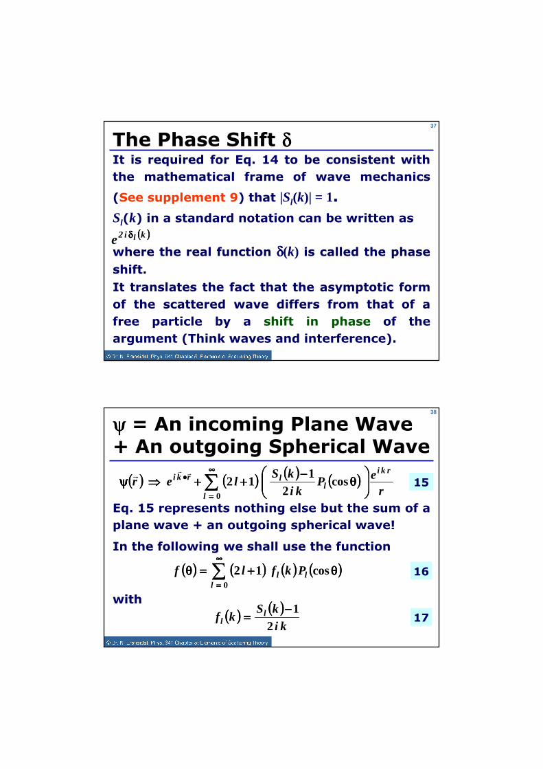
It is required for Eq. 14 to be consistent with the mathematical frame of wave mechanics

(See supplement 9) that |Sl(k)| = 1.

The Phase Shift δδδδ

Sl(k) in a standard notation can be written as(((( ))))ki2 le δδδδ

where the real function δδδδ(k) is called the phase shift.It translates the fact that the asymptotic form of the scattered wave differs from that of a free particle by a shift in phase of the argument (Think waves and interference).

38

Eq. 15 represents nothing else but the sum of a plane wave + an outgoing spherical wave!

In the following we shall use the function

with

ψψψψ = An incoming Plane Wave + An outgoing Spherical Wave

(((( )))) (((( )))) (((( )))) (((( ))))∑∑∑∑∞∞∞∞

====θθθθ++++====θθθθ

0

cos12l

ll Pkflf 16

(((( )))) (((( )))) (((( )))) (((( ))))r

ePki

kSler

rki

ll

lrki ∑∑∑∑∞∞∞∞

====

••••

θθθθ

−−−−++++++++⇒⇒⇒⇒ψψψψ0

cos2

112

rrr15

(((( )))) (((( ))))ki

kSkf l

l 21−−−−==== 17

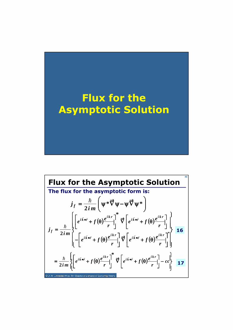
Flux for the Asymptotic Solution

40

The flux for the asymptotic form is:

16

17

Flux for the Asymptotic Solution

ψψψψ∇∇∇∇ψψψψ−−−−ψψψψ∇∇∇∇ψψψψ====→→→→→→→→

**2 mi

j fh

(((( )))) (((( ))))

(((( )))) (((( ))))

θθθθ++++∇∇∇∇

θθθθ++++−−−−

θθθθ++++∇∇∇∇

θθθθ++++

====••••→→→→••••

••••→→→→••••

*

*

2

refe

refe

refe

refe

mij

rkirki

rkirki

rkirki

rkirki

frrrr

rrrr

h

(((( )))) (((( ))))

−−−−

θθθθ++++∇∇∇∇

θθθθ++++==== ••••→→→→•••• cc

refe

refe

mi

rkirki

rkirki

rrrrh*

2

41

We shall skip some steps in order to calculate jf and leave this as a homework.

2)Then calculating the gradient.

1) First using .θθθθ====•••• cosrkrkrr

3) Neglecting the terms in r3 since they are dominated by the 1/r2 for large r.This is largely justified by the fact that we are interested in the flux far away from the interaction region (where the potential is localized), i.e. at large r (see fig. 5-4)

Calculating jf

42

Calculating jf - Steps

4) Finally considering a scattering angle θθθθ#0.

This is also justified by the fact that the detector is always placed at an angle and in a measurement (Rutherford) we want the integrated flux over a small but finite solid angle (Rutherford scattering).5) Finally using Riemann-Lebesgue Lemma when integrating over the small but finite solid angle.

See Supplement 9 and Problem 7 of chapter 19 - in Gasiorowicz

43

jf

The result is the following expression for jf

is the unit vector in the direction of ri→→→→r

18(((( ))))

2

2ˆ

r

fi

mk

mk

j rfθθθθ

++++====→→→→

hh

44

jf - Discussion

18(((( ))))

2

2ˆ

r

fi

mk

mk

j rfθθθθ

++++====→→→→

hh

First remark: it is obvious that in the absence of a “scattering” potential, the 2nd

term on the right in eq. 18 vanishes and we retrieve the expression of the incident flux (eq. 13)

45

Discussion – The First Term1

18(((( ))))

2

2ˆ

r

fi

mk

mk

j rfθθθθ

++++====→→→→

hh

For the radial flux, i.e the first term

gives a contribution . mk

ir

→→→→

•••• hˆ

θθθθcosmkh

In a wave-packet treatment, would be

multiplied by a function which defines the

lateral dimensions of the beam.

mk→→→→

h

46

Discussion – The First Term2

This contribution is only significant in the forward region within a finite region of the z-axis. And since the detector is placed far outside this region we can consider that the first term does not contribute to the radial flux in the asymptotic region.

Asymptotic region

Cross Section

48

Flux → → → → Number of Particles

Translating the asymptotic flux jf into number of outgoing scattered particles (per time unit) we write:

19(((( ))))

ΩΩΩΩθθθθ

≈≈≈≈••••==== drr

f

mk

dAijdN rf2

2

2

ˆ h

Important remark: the factor r2 vanishes and this is, a posteriori, a justification of having neglected the terms in r3.

49

Differential Cross SectionThe differential cross section is defined by:

20

(((( ))))(((( )))) 2

22

2

θθθθ====ΩΩΩΩ

ΩΩΩΩθθθθ

≈≈≈≈ΩΩΩΩ

====ΩΩΩΩσσσσ

fd

mk

drr

f

mk

djdN

dd

i h

h

Compare with the classical definition of the differential cross section in supplement 8.

50

If the potential has a spin dependence, as it is the case for the nucleon-nucleon interaction then there may be an azimuthal dependence. Eq. 20 is generalized in this case and we write:

Spin Dependence

21(((( )))) 2,φφφφθθθθ====

ΩΩΩΩσσσσ

fdd

51

The total cross section of the scattering process is obtained by integrating over all possible values of θθθθ, i.e. of dΩΩΩΩ

Total Cross Section

22(((( )))) (((( )))) ΩΩΩΩφφφφθθθθ====ΩΩΩΩΩΩΩΩσσσσ====σσσσ ∫∫∫∫∫∫∫∫∫∫∫∫∫∫∫∫ dfd

ddktot

2,

52

One can show that, and we leave this as a homework, :

Total Cross Section

23(((( )))) (((( ))))∑∑∑∑∞∞∞∞

====δδδδππππ====σσσσ

0

22 sin

4

lltot k

kk

53

If one considers f(0), (see eqs. 16 & 17) i.e:

The Optical Theorem1

(((( )))) (((( )))) (((( )))) (((( ))))∑∑∑∑∞∞∞∞

====

−−−−++++====0

12

1120

ll

l Pki

kSlf 24

(((( )))) (((( ))))(((( ))))

(((( ))))∑∑∑∑∞∞∞∞

====

δδδδ

−−−−++++====0

2

12

1120

ll

ki

Pki

elf 25

(((( )))) (((( )))) (((( ))))(((( )))) (((( ))))

(((( ))))∑∑∑∑∞∞∞∞

====

δδδδδδδδδδδδ

−−−−++++====0

12

1210l

l

kikiki P

iee

elk

f 26

(((( )))) (((( )))) (((( )))) (((( )))) (((( ))))∑∑∑∑∞∞∞∞

====

δδδδ δδδδ++++====0

1sin1210l

lki Pkel

kf 27

54

Comparing with the expression of the total cross section;

we have:

Taking the imaginary part of eq. 27, we have:

The Optical Theorem2

(((( ))))(((( )))) (((( )))) (((( ))))∑∑∑∑∞∞∞∞

====δδδδ++++====

0

2sin1210Iml

klk

f 28

23(((( )))) (((( ))))∑∑∑∑

∞∞∞∞

====δδδδππππ====σσσσ

0

22 sin

4

lltot k

kk

(((( )))) (((( ))))kkf totσσσσππππ

====4

0Im 29

55

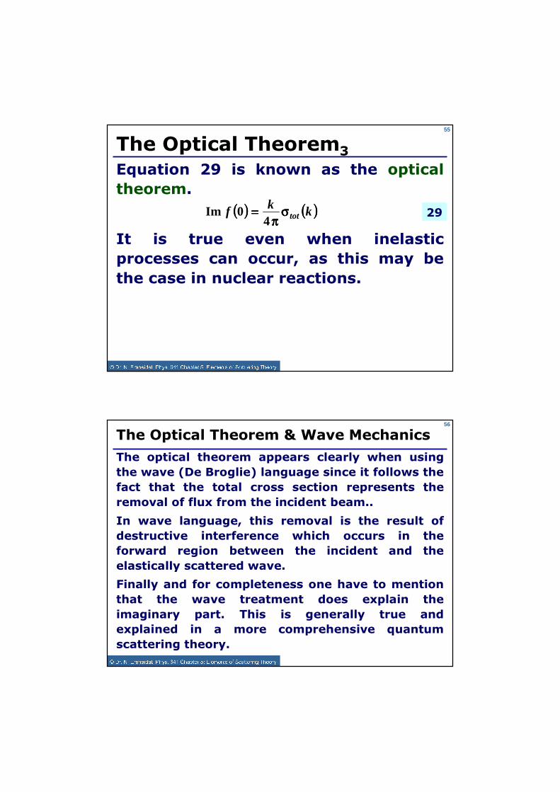
It is true even when inelastic processes can occur, as this may be the case in nuclear reactions.

Equation 29 is known as the optical theorem.

The Optical Theorem3

29(((( )))) (((( ))))kkf totσσσσππππ

====4

0Im

56

In wave language, this removal is the result of destructive interference which occurs in the forward region between the incident and the elastically scattered wave.

The optical theorem appears clearly when using the wave (De Broglie) language since it follows the fact that the total cross section represents the removal of flux from the incident beam..

The Optical Theorem & Wave Mechanics

Finally and for completeness one have to mention that the wave treatment does explain the imaginary part. This is generally true and explained in a more comprehensive quantum scattering theory.

5555----5555 Scattering Stationary Scattering Stationary Scattering Stationary Scattering Stationary States States States States –––– Other ApproachOther ApproachOther ApproachOther Approach5555----5555 Scattering Stationary Scattering Stationary Scattering Stationary Scattering Stationary States States States States –––– Other ApproachOther ApproachOther ApproachOther Approach

End of Lecture 18

Next Lecture

Reference: Paragraphs B and CQuantum Mechanics, Vol. 2 Chapter VIIIC. Cohen-Tannoudji, B. Diu and F. Laloë