Yapparova, A., Gabellone, T., Whitaker, F., Kulik, D. A., & Matthäi, S.K. (2017). Reactive transport modelling of hydrothermal dolomitisationusing the CSMP++GEM coupled code: Effects of temperature andgeological heterogeneity. Chemical Geology, 466, 562-574.https://doi.org/10.1016/j.chemgeo.2017.07.005

Peer reviewed versionLicense (if available):CC BY-NC-NDLink to published version (if available):10.1016/j.chemgeo.2017.07.005

Link to publication record in Explore Bristol ResearchPDF-document

This is the author accepted manuscript (AAM). The final published version (version of record) is available onlinevia Elsevier at http://www.sciencedirect.com/science/article/pii/S0009254117304035. Please refer to anyapplicable terms of use of the publisher.

University of Bristol - Explore Bristol ResearchGeneral rights

This document is made available in accordance with publisher policies. Please cite only thepublished version using the reference above. Full terms of use are available:http://www.bristol.ac.uk/red/research-policy/pure/user-guides/ebr-terms/

Reactive transport modelling of hydrothermal

dolomitisation using the CSMP++GEM coupled code:

Effects of temperature and geological heterogeneity

Alina Yapparovaa,∗, Tatyana Gabelloneb, Fiona Whitakerb, Dmitrii A.Kulika, Stephan K. Matthaic

aPaul Scherrer Institute, Laboratory for Waste Management, 5232 Villigen PSI,Switzerland

bUniversity of Bristol, School of Earth Sciences, Wills Memorial Building, Queen’s Road,Bristol, BS8 1RJ, UK

cUniversity of Melbourne, School of Engineering, Melbourne, 3010, Australia

Abstract

Reactive transport simulations using our CSMP++GEM coupled codewere applied to study the major controls on replacement dolomitisation andthe development of dolomite geobodies in a hydrothermal setting. A seriesof 2D simulations show how elevated temperature and reactive surface areaincrease the rate of dolomitisation, and result in a dolomite replacement frontthat is both sharper and inclined at a higher angle from vertical. This in-clination, an effect of gravity segregation, is apparent in thick homogeneousunits, but in layered systems the lithological contrast determines the shapeof the dolomite front. The increase in permeability resulting from porositygeneration upon replacement of calcite by dolomite has a major effect on ac-celerating the overall progress of dolomitisation. In contrast, the changes influid density due to chemical reactions and the pressure dependence of ther-modynamic data have a minor influence under simulated conditions. Primarydolomite forms slowly after complete replacement of host calcite, leading toporosity decrease, and is only locally important around the source of thehydrothermal fluid.

For a simple layered system, our model results are in excellent agreement

∗

Corresponding author. Present address: ETH Zurich, Institute of Geochemistry andPetrology. E-mail address: alina.yapparova@gmail.com

Preprint submitted to Chemical Geology July 6, 2017

with those obtained using TOUGHREACT code. They do, however, showthe advantage of unstructured triangular over structured rectangular meshesfor resolving complex curved/inclined front shapes. Such meshes also offerbenefits in simulating fault-controlled hydrothermal dolomitisation.

Our simulations predict dolomite geobodies comparable in scale and mor-phology to natural examples documented at outcrops, and underline the im-portance of understanding the permeability structure within and around thefault zone.

Keywords:reactive transport modelling, hydrothermal dolomitisation, Gibbs energyminimization, finite element – finite volume method, unstructured grids

1. Introduction

Reactive transport modelling (RTM), which couples fluid flow and geo-chemical reactions along flow paths, is an emerging numerical tool which canbe used to identify and quantify major controls on water-rock interaction,and can help to improve predictions of diagenetic modification of reservoirquality (Steefel et al., 2005; Agar and Geiger, 2015). Reactive transport phe-nomena involve the synergistic interplay of simultaneous chemical reactionsand fluid transport in geologically heterogeneous rocks, which is not possibleto understand with the help of transport-only or chemical speciation-onlymodels.

RTM has already been extensively applied to study the formation ofdolomites in low-temperature shallow reflux systems (Jones and Xiao, 2005;Garcia-Fresca et al., 2009; Al-Helal et al., 2012; Xiao et al., 2013; Gabelloneand Whitaker, 2016; Gabellone et al., 2016; Lu and Cantrell, 2016), as wellas during burial diagenesis by fluids circulating due to geothermal convection(Wilson et al., 2001; Whitaker and Xiao, 2010) and sedimentary compaction(Consonni et al., 2010; Frazer et al., 2014).

By contrast to these diagenetic environments, there have only been alimited number of RTM studies of dolomitisation driven by circulation of hy-drothermal fluids. Nonetheless, hydrothermal dolomites (HTD) are of con-siderable economic interest as they can form targets for hydrocarbon pro-duction (Davies and Smith, 2006), or occur in association with MississippiValley-type (MVT) ore bodies (Qing and Mountjoy, 1994; Davies and Smith,2006).

2

Hydrothermal dolomites form by ingress into a fault zone of Mg-rich fluidswith a temperature that is elevated (by 5-10C) relative to the host limestone(Machel and Lonnee, 2002), and are usually structurally controlled. HTDbodies can have a patchy and localised distribution around sub-seismic scalefaults (Machel, 2004; Wilson et al., 2007; Lopez-Horgue et al., 2010), butcan also occur as stratabound bodies extending laterally for several tens ofkilometres away from the faults proposed to have sourced the hydrothermalfluids (Davies and Smith, 2006; Corbella et al., 2014; Dewit et al., 2014). Im-portant uncertainties remain as to the controls on the nature of hydrothermalalteration and the extent to which this process can form laterally extensivedolomites. Alteration can either increase or reduce porosity and permeabil-ity, and prediction of the spatial distribution of hydrothermal dolomites canbe challenging.

RTM simulations by Corbella et al. (2014) explored major controlling pa-rameters on the development of stratabound dolomite bodies associated withfault-controlled hydrothermal fluids in the Benicassim area (Maestrat Basin,eastern Spain). They concluded that layers with differences in permeabilityof two orders of magnitude are needed in order to produce the observed kilo-meter long dolomite bodies within the more permeable packstone-grainstonebeds. The employed fluid (five times concentrated seawater at 100 C) ispreferentially focused in these more permeable layers with lateral fluxes ofseveral meters per year.

Consonni et al. (2016) simulated hydrothermal dolomitisation occurringin a lacustrine limestone reservoir of the Toca Formation (West Africa) andidentified permeability as the major control on the distribution of dolomi-tised bodies. These authors also recognised the importance of flow rate, flowduration and fluid composition in determining the lateral extent of dolomi-tisation away from the faults. By doubling the flow rate or the simulationtime the volume of the completely dolomitised limestone was almost dou-bled. Similar conclusions were reached by Jones et al. (2010) whose 2D and3D simulations of HTD show preferential dolomitisation of the hanging wallof the fault blocks and a strong control on the dolomitisation pattern by faultand matrix permeability variations as well as by brine composition.

Fault-related hydrothermal diagenesis was simulated in generic sub-seismicscale RTMs (Xiao et al., 2013), with Mg-rich hydrothermal fluids flowingthrough a simple rectilinear fault over tens of thousands of years leading tolarge scale HTD formation and significant reservoir quality modification.

Although a few RTM studies of hydrothermal dolomitisation have been

3

reported, the effect of some numerical solution features on the resultingdolomite bodies has not been studied in detail. For example, Corbellaet al. (2014) performed a sensitivity analysis on the influence of temperatureon the rate of dolomitisation, but the RTM code RETRASO used in theirstudy did not include the permeability update from changing porosity. BothCSMP++GEM (Yapparova et al., 2017) and TOUGHREACT (Xu et al.,2004) have this feature implemented. Other features of CSMP++GEM,such as the dependence of thermodynamic data on fluid pressure, and offluid properties on chemistry, are also lacking in many other RTMs.

This study has the twofold aim of (i) better understanding the main con-trols on rates and patterns of hydrothermal fault-controlled dolomitisation,and (ii) exploring the applicability of different numerical solution proceduresin reactive transport modelling.

A model with homogeneous rock properties and another with two layersof contrasting permeability were set up in CSMP++GEM in order to explorehow RTM results are affected by the mesh type and refinement, and by thepermeability feedback on the flow. In particular, we aimed to discriminatebetween ”true” modelling results and artefacts due to the employed numericalprocedure and/or modelling set up. The results of the homogeneous referencemodel in CSMP++GEM were compared with those from a similar modelbuilt in TOUGHREACT.

We then used CSMP++GEM to simulate HTD development in a layeredand faulted limestone system, using different fault geometries (with verticaland inclined fault planes) to examine controls on specific aspects of the geom-etry of dolomite bodies. Specifically, we intended to address these questions:

1. What are the main controls on the width and the inclination of thedolomitisation fronts?

2. In HTD systems, what controls the development of stratabound vsmassive dolomite bodies?

3. How does the geometry of the fluid-sourcing fault and the presence ofa sealing layer influence the dolomitisation pattern?

The paper ends with a discussion comparing HTD bodies predicted by ourreactive transport simulations with those from Corbella et al. (2014), andwith natural examples from various outcrops.

4

2. Methods

2.1. Reactive transport model

The new CSMP++GEM reactive transport code (Yapparova et al., 2017)was applied to simulate hydrothermal dolomitisation in 2D. A subset of mod-els also uses TOUGHREACT (Xu et al., 2004) in order to provide a com-parison between the codes.

CSMP++ allows flow simulations with transient pressure including grav-ity effects. It contains a mass conservative transport scheme and an accurateequation of state for saline water (Driesner and Heinrich, 2007). Govern-ing equations for fluid flow and solute transport are solved using the finiteelement – finite volume method (Geiger et al., 2004).

Chemical equilibrium calculations at different temperatures and pressuresare performed by means of the GEMS3K standalone kernel (Kulik et al.,2013). The kinetic rate of mineral precipitation is incorporated into theequilibrium calculations via the additional metastability constraints on min-eral amounts (for a detailed description see Thien et al., 2014; Yapparovaet al., 2017).

Transport-chemistry coupling is performed following the Sequential Non-iterative Approach (SNIA)(de Dieuleveult et al., 2009) and includes the feed-back of the diagenetic change in porosity and permeability. Porosity is up-dated based on the current mineral volumes, permeability is updated from theporosity using Kozeny-Carman empirical relation (Yapparova et al., 2017):

kn+1 = kn(1 − φn)2(φn+1)3

(1 − φn+1)2(φn)3, (1)

where kn+1 and φn+1 are the permeability and the porosity at the next timestep, respectively, and kn and φn at the current time step.

The rate of calcite dissolution is orders of magnitude higher than therate of dolomite precipitation, and thus in our simulations dolomite was akinetically controlled mineral, and calcite was under thermodynamic control.The kinetic rate of dolomite dissolution/precipitation (in mol/s) was takenfrom Arvidson and Mackenzie (1999):

r = κA(1 − Ω)η, (2)

where Ω is the ratio between the ion activity product and the solubilityproduct (logΩ = SI, mineral saturation index), η = 2.26 is the reaction order,

5

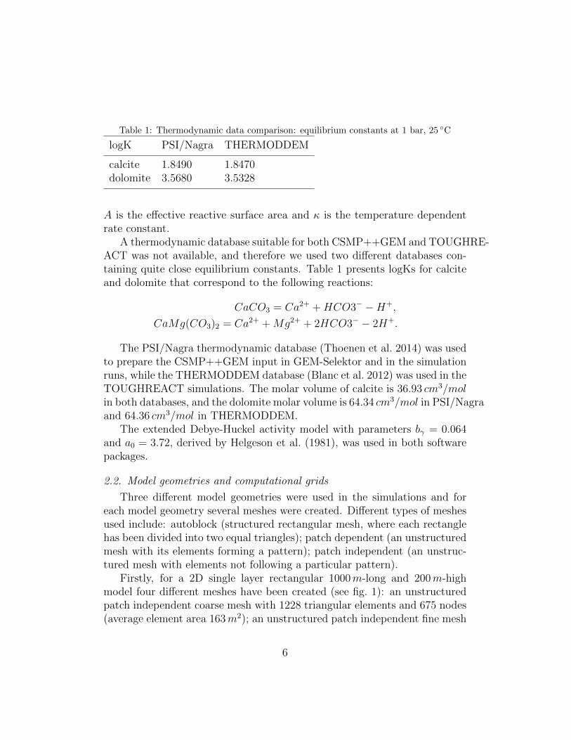
Table 1: Thermodynamic data comparison: equilibrium constants at 1 bar, 25 C

logK PSI/Nagra THERMODDEM

calcite 1.8490 1.8470dolomite 3.5680 3.5328

A is the effective reactive surface area and κ is the temperature dependentrate constant.

A thermodynamic database suitable for both CSMP++GEM and TOUGHRE-ACT was not available, and therefore we used two different databases con-taining quite close equilibrium constants. Table 1 presents logKs for calciteand dolomite that correspond to the following reactions:

CaCO3 = Ca2+ +HCO3− −H+,

CaMg(CO3)2 = Ca2+ +Mg2+ + 2HCO3− − 2H+.

The PSI/Nagra thermodynamic database (Thoenen et al. 2014) was usedto prepare the CSMP++GEM input in GEM-Selektor and in the simulationruns, while the THERMODDEM database (Blanc et al. 2012) was used in theTOUGHREACT simulations. The molar volume of calcite is 36.93 cm3/molin both databases, and the dolomite molar volume is 64.34 cm3/mol in PSI/Nagraand 64.36 cm3/mol in THERMODDEM.

The extended Debye-Huckel activity model with parameters bγ = 0.064and a0 = 3.72, derived by Helgeson et al. (1981), was used in both softwarepackages.

2.2. Model geometries and computational grids

Three different model geometries were used in the simulations and foreach model geometry several meshes were created. Different types of meshesused include: autoblock (structured rectangular mesh, where each rectanglehas been divided into two equal triangles); patch dependent (an unstructuredmesh with its elements forming a pattern); patch independent (an unstruc-tured mesh with elements not following a particular pattern).

Firstly, for a 2D single layer rectangular 1000m-long and 200m-highmodel four different meshes have been created (see fig. 1): an unstructuredpatch independent coarse mesh with 1228 triangular elements and 675 nodes(average element area 163m2); an unstructured patch independent fine mesh

6

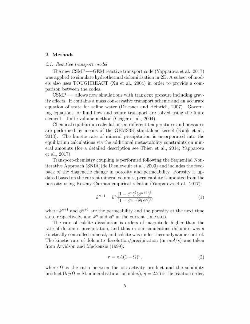
with 2674 triangular elements and 1398 nodes (average 75m2); an unstruc-tured patch dependent mesh with 1214 triangular elements and 669 nodes(average 165m2); a structured mesh with 1166 right-angled triangles and648 nodes (average 171m2). For comparison a homogeneous model was alsodeveloped in TOUGHREACT, with three uniform grids of 20, 10 and 5msize (500, 2000 and 8000 cells with areas of 400, 100 and 25 m2, respectively).

c)a)

b) d)

Figure 1: (a) unstructured coarse mesh, (b) unstructured fine mesh, (c) patch dependentmesh, (d) structured mesh

Secondly, for a 2D rectangular 500m-long and 100m-high model withtwo layers each 50m-thick two unstructured patch dependent meshes werecreated (see fig. 2): one with the uniform cell size (1711 triangles and 940nodes with average cells of 117m2) and the other one with a refinement alongthe boundary between the two layers (2486 triangles and 1309 nodes withaverage cells of 80m2).

a)

b)

Figure 2: (a) uniform mesh and (b) mesh refined at the boundary between the highpermeability and low permeability layers

Thirdly, a layered model geometry bisected by a fault extending from thetop to the bottom of the grid was adapted from Corbella et al. (2014). It

7

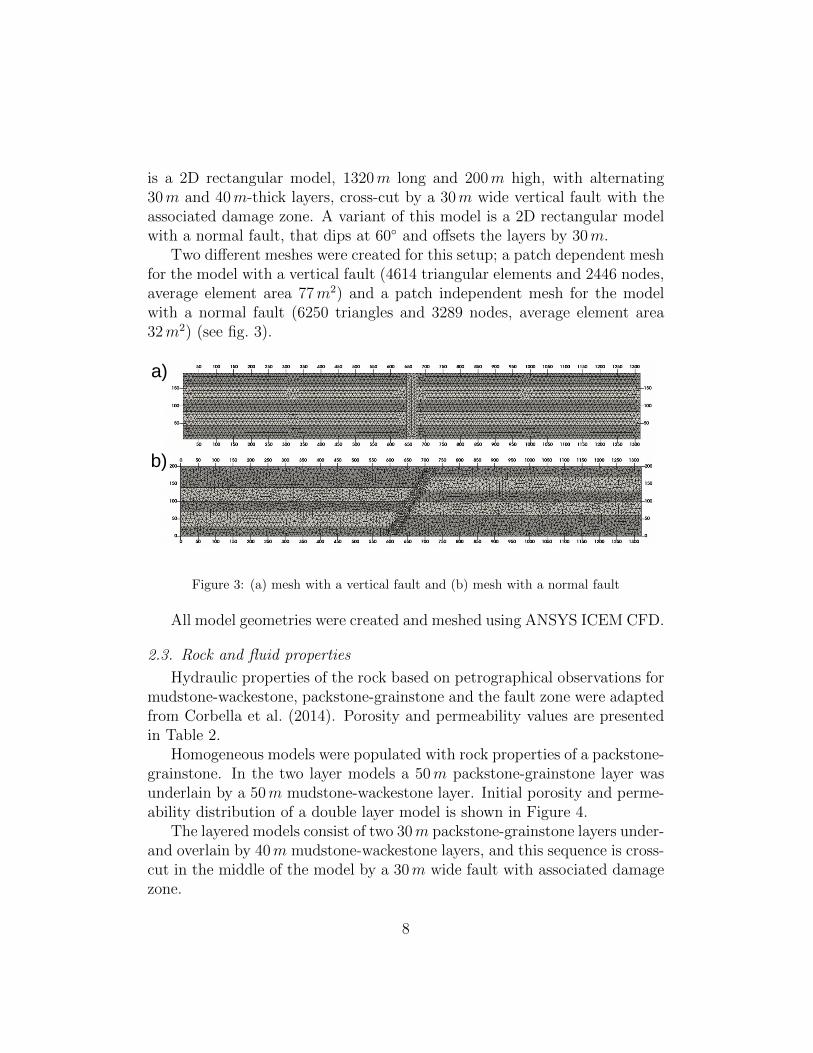
is a 2D rectangular model, 1320m long and 200m high, with alternating30m and 40m-thick layers, cross-cut by a 30m wide vertical fault with theassociated damage zone. A variant of this model is a 2D rectangular modelwith a normal fault, that dips at 60 and offsets the layers by 30m.

Two different meshes were created for this setup; a patch dependent meshfor the model with a vertical fault (4614 triangular elements and 2446 nodes,average element area 77m2) and a patch independent mesh for the modelwith a normal fault (6250 triangles and 3289 nodes, average element area32m2) (see fig. 3).

a)

b)

Figure 3: (a) mesh with a vertical fault and (b) mesh with a normal fault

All model geometries were created and meshed using ANSYS ICEM CFD.

2.3. Rock and fluid properties

Hydraulic properties of the rock based on petrographical observations formudstone-wackestone, packstone-grainstone and the fault zone were adaptedfrom Corbella et al. (2014). Porosity and permeability values are presentedin Table 2.

Homogeneous models were populated with rock properties of a packstone-grainstone. In the two layer models a 50m packstone-grainstone layer wasunderlain by a 50m mudstone-wackestone layer. Initial porosity and perme-ability distribution of a double layer model is shown in Figure 4.

The layered models consist of two 30m packstone-grainstone layers under-and overlain by 40m mudstone-wackestone layers, and this sequence is cross-cut in the middle of the model by a 30m wide fault with associated damagezone.

8

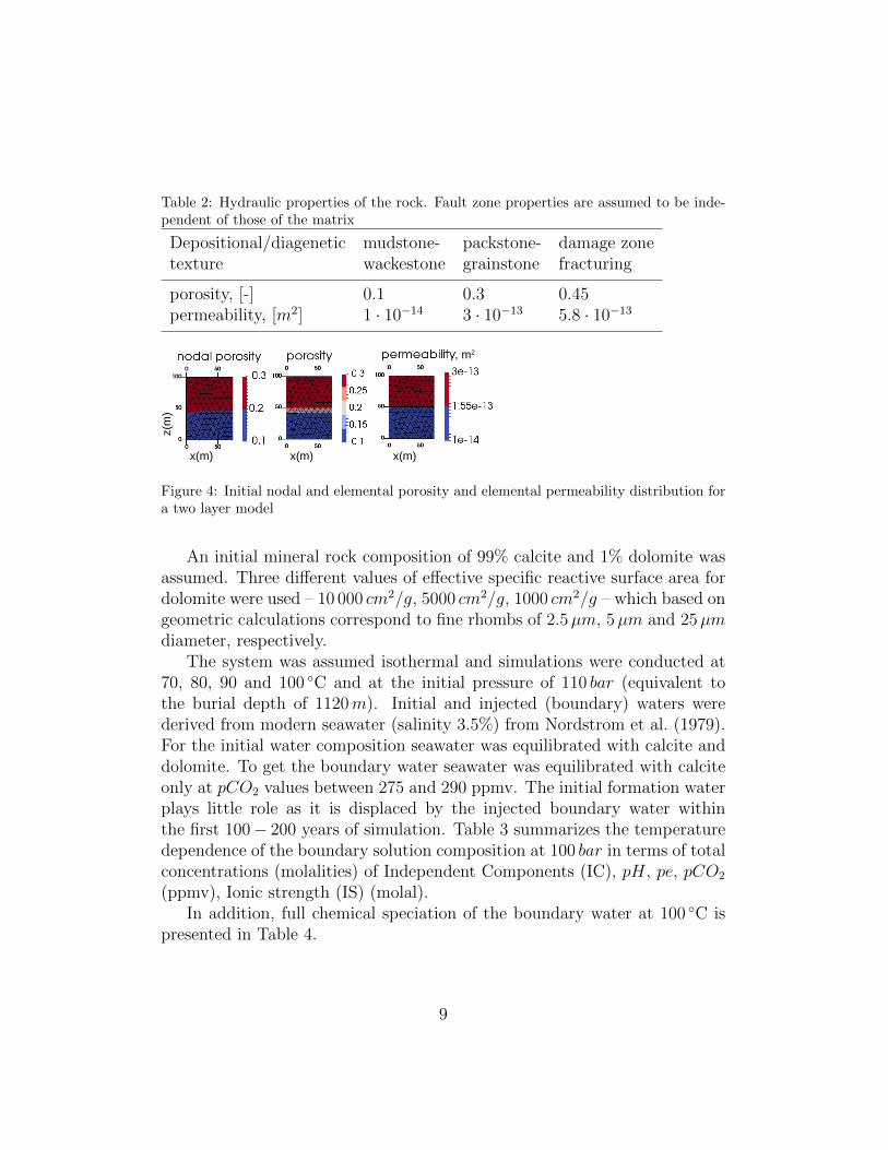
Table 2: Hydraulic properties of the rock. Fault zone properties are assumed to be inde-pendent of those of the matrix

Depositional/diagenetic mudstone- packstone- damage zonetexture wackestone grainstone fracturing

porosity, [-] 0.1 0.3 0.45permeability, [m2] 1 · 10−14 3 · 10−13 5.8 · 10−13

x(m) x(m) x(m)

z(m

)

, m2

Figure 4: Initial nodal and elemental porosity and elemental permeability distribution fora two layer model

An initial mineral rock composition of 99% calcite and 1% dolomite wasassumed. Three different values of effective specific reactive surface area fordolomite were used – 10 000 cm2/g, 5000 cm2/g, 1000 cm2/g – which based ongeometric calculations correspond to fine rhombs of 2.5µm, 5µm and 25µmdiameter, respectively.

The system was assumed isothermal and simulations were conducted at70, 80, 90 and 100 C and at the initial pressure of 110 bar (equivalent tothe burial depth of 1120m). Initial and injected (boundary) waters werederived from modern seawater (salinity 3.5%) from Nordstrom et al. (1979).For the initial water composition seawater was equilibrated with calcite anddolomite. To get the boundary water seawater was equilibrated with calciteonly at pCO2 values between 275 and 290 ppmv. The initial formation waterplays little role as it is displaced by the injected boundary water withinthe first 100 − 200 years of simulation. Table 3 summarizes the temperaturedependence of the boundary solution composition at 100 bar in terms of totalconcentrations (molalities) of Independent Components (IC), pH, pe, pCO2

(ppmv), Ionic strength (IS) (molal).In addition, full chemical speciation of the boundary water at 100 C is

presented in Table 4.

9

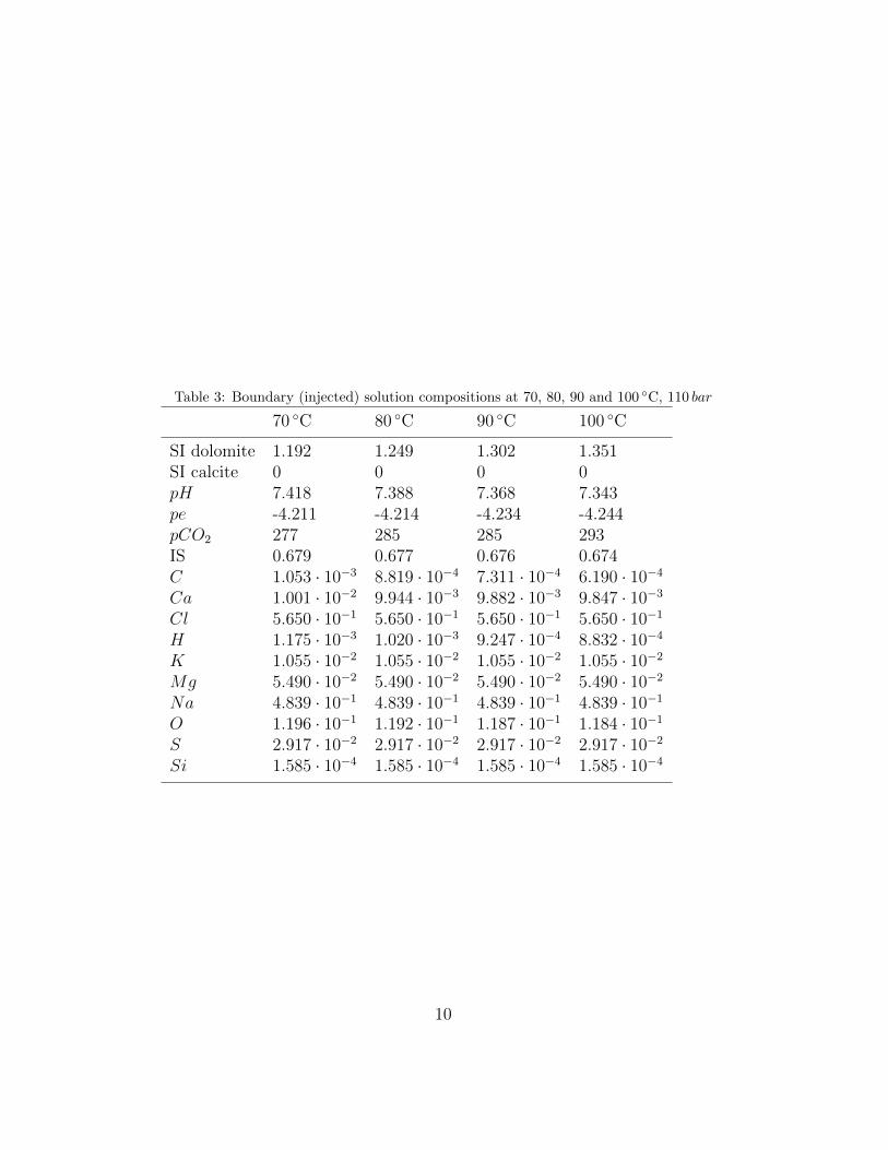
Table 3: Boundary (injected) solution compositions at 70, 80, 90 and 100 C, 110 bar

70 C 80 C 90 C 100 C

SI dolomite 1.192 1.249 1.302 1.351SI calcite 0 0 0 0pH 7.418 7.388 7.368 7.343pe -4.211 -4.214 -4.234 -4.244pCO2 277 285 285 293IS 0.679 0.677 0.676 0.674C 1.053 · 10−3 8.819 · 10−4 7.311 · 10−4 6.190 · 10−4

Ca 1.001 · 10−2 9.944 · 10−3 9.882 · 10−3 9.847 · 10−3

Cl 5.650 · 10−1 5.650 · 10−1 5.650 · 10−1 5.650 · 10−1

H 1.175 · 10−3 1.020 · 10−3 9.247 · 10−4 8.832 · 10−4

K 1.055 · 10−2 1.055 · 10−2 1.055 · 10−2 1.055 · 10−2

Mg 5.490 · 10−2 5.490 · 10−2 5.490 · 10−2 5.490 · 10−2

Na 4.839 · 10−1 4.839 · 10−1 4.839 · 10−1 4.839 · 10−1

O 1.196 · 10−1 1.192 · 10−1 1.187 · 10−1 1.184 · 10−1

S 2.917 · 10−2 2.917 · 10−2 2.917 · 10−2 2.917 · 10−2

Si 1.585 · 10−4 1.585 · 10−4 1.585 · 10−4 1.585 · 10−4

10

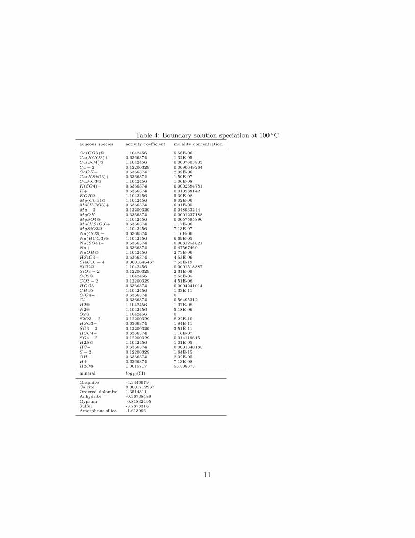
Table 4: Boundary solution speciation at 100 Caqueous species activity coefficient molality concentration

Ca(CO3)@ 1.1042456 5.58E-06Ca(HCO3)+ 0.6366374 1.32E-05Ca(SO4)@ 1.1042456 0.0007603803Ca + 2 0.12200329 0.0090649264CaOH+ 0.6366374 2.92E-06Ca(HSiO3)+ 0.6366374 1.59E-07CaSiO3@ 1.1042456 1.06E-08K(SO4)− 0.6366374 0.0002584781K+ 0.6366374 0.010288142KOH@ 1.1042456 5.39E-08Mg(CO3)@ 1.1042456 9.02E-06Mg(HCO3)+ 0.6366374 6.91E-05Mg + 2 0.12200329 0.048933244MgOH+ 0.6366374 0.0001237188MgSO4@ 1.1042456 0.0057595896Mg(HSiO3)+ 0.6366374 1.17E-06MgSiO3@ 1.1042456 7.13E-07Na(CO3)− 0.6366374 1.16E-06Na(HCO3)@ 1.1042456 6.69E-05Na(SO4)− 0.6366374 0.0081254821Na+ 0.6366374 0.47567469NaOH@ 1.1042456 2.73E-06HSiO3− 0.6366374 4.53E-06Si4O10 − 4 0.0001645467 7.53E-19SiO2@ 1.1042456 0.0001518887SiO3 − 2 0.12200329 2.31E-09CO2@ 1.1042456 2.55E-05CO3 − 2 0.12200329 4.51E-06HCO3− 0.6366374 0.0004241014CH4@ 1.1042456 1.33E-11ClO4− 0.6366374 0Cl− 0.6366374 0.56495312H2@ 1.1042456 1.07E-08N2@ 1.1042456 5.18E-06O2@ 1.1042456 0S2O3 − 2 0.12200329 8.22E-10HSO3− 0.6366374 1.84E-11SO3 − 2 0.12200329 3.51E-11HSO4− 0.6366374 1.16E-07SO4 − 2 0.12200329 0.014119615H2S@ 1.1042456 1.01E-05HS− 0.6366374 0.0001340185S − 2 0.12200329 1.64E-15OH− 0.6366374 2.02E-05H+ 0.6366374 7.13E-08H2O@ 1.0015717 55.508373

mineral log10(SI)

Graphite -4.3446979Calcite 0.0001712937Ordered dolomite 1.3514311Anhydrite -0.36738489Gypsum -0.81832495Sulfur -3.7878316Amorphous silica -1.613096

11

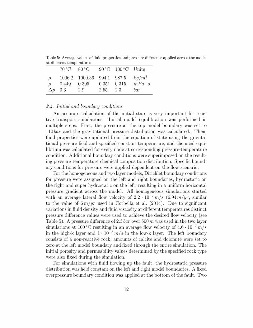
Table 5: Average values of fluid properties and pressure difference applied across the modelat different temperatures

70 C 80 C 90 C 100 C Units

ρ 1006.2 1000.36 994.1 987.5 kg/m3

µ 0.449 0.395 0.351 0.315 mPa · s∆p 3.3 2.9 2.55 2.3 bar

2.4. Initial and boundary conditions

An accurate calculation of the initial state is very important for reac-tive transport simulations. Initial model equilibration was performed inmultiple steps. First, the pressure at the top model boundary was set to110 bar and the gravitational pressure distribution was calculated. Then,fluid properties were updated from the equation of state using the gravita-tional pressure field and specified constant temperature, and chemical equi-librium was calculated for every node at corresponding pressure-temperaturecondition. Additional boundary conditions were superimposed on the result-ing pressure-temperature-chemical composition distribution. Specific bound-ary conditions for pressure were applied dependent on the flow scenario.

For the homogeneous and two layer models, Dirichlet boundary conditionsfor pressure were assigned on the left and right boundaries, hydrostatic onthe right and super hydrostatic on the left, resulting in a uniform horizontalpressure gradient across the model. All homogeneous simulations startedwith an average lateral flow velocity of 2.2 · 10−7m/s (6.94m/yr, similarto the value of 6m/yr used in Corbella et al. (2014). Due to significantvariations in fluid density and fluid viscosity at different temperatures distinctpressure difference values were used to achieve the desired flow velocity (seeTable 5). A pressure difference of 2.3 bar over 500m was used in the two layersimulations at 100 C resulting in an average flow velocity of 4.6 · 10−7m/sin the high-k layer and 1 · 10−8m/s in the low-k layer. The left boundaryconsists of a non-reactive rock, amounts of calcite and dolomite were set tozero at the left model boundary and fixed through the entire simulation. Theinitial porosity and permeability values determined by the specified rock typewere also fixed during the simulation.

For simulations with fluid flowing up the fault, the hydrostatic pressuredistribution was held constant on the left and right model boundaries. A fixedoverpressure boundary condition was applied at the bottom of the fault. Two

12

sets of simulations were performed: with a top boundary open for the outflow(constant pressure of 110 bar assigned), and with a closed top boundary. Anoverpressure of 2.9 bar (compared to the hydrostatic pressure value) at thebottom of the fault results in average flow velocities on the order of 10−6m/sin the fault zone, 10−7m/s in the high-k layers and 10−8m/s in the low-klayers.

2.5. Time stepping

The Courant–Friedrichs–Lewy (CFL) condition is a necessary conditionfor convergence of a numerical solution of the transport equation. It is a timestep restriction, that ensures that the fluid will move not more that one gridcell during a single time step. This is of particular importance for reactivetransport simulations that use Sequential Non-Iterative Approach (SNIA).On one hand, the time step should be big enough for the fluid to reactwith the rock before it leaves the cell, on the other, if the time step of thetransport-chemistry coupling is too small (much less than the one providedby CFL calculations) the fluid will react with the rock several times beforeleaving the cell and the amount of dissolved/precipitated minerals will beoverestimated.

Simulations were carried out for time periods of tens of thousands of yearswith two nested time stepping loops. The pressure field was updated every10 years and solute transport and chemical equilibrium/kinetic calculationswere performed with a CFL restricted time step. Thus, for a homogeneoussimulation CFL varied from ∼ 200 days in the beginning of the simulationto ∼ 50 days after complete dolomitisation.

3. Results

3.1. Comparison of CSMP++GEM and TOUGHREACT runs

Our reference simulation was conducted at 100 C using all model features(porosity feedback, permeability feedback, salinity feedback, pressure depen-dence of chemistry) on a coarse unstructured grid (fig. 1a). The 1000m-longand 200m-high model was populated with the rock properties of a packstone-grainstone and dolomite RSA was set to 10 000 cm2/g.

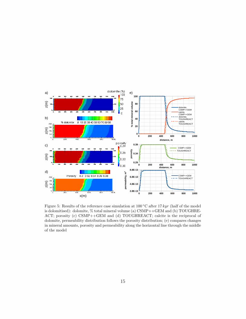
The results were compared to those obtained with TOUGHREACT on agrid with 20×20m cell size (see fig. 5). A close match was achieved, with theposition of the dolomite front in TOUGHREACT being very slightly ahead of

13

the one from CSMP++GEM. After 17 kyr of simulation time, 50 vol% of cal-cite is replaced by dolomite. Dolomite precipitation drives calcite dissolution,generating up to 9% additional porosity, and increasing permeability up to8.6 ·10−13m2 (almost three times higher than the initial value of 3 ·10−13m2).The dolomite front is inclined, advancing more rapidly near the top of themodel. Porosity reduction caused by primary dolomite cement precipitationafter complete calcite replacement is prominent in the vertical zone over thefirst 50m close to the injection point (left boundary). Horizontal flow ve-locity increases from the average value of 2.2 · 10−7m/s in the beginning ofthe simulation to an average of 3.4 · 10−7m/s after 17 kyr. Flow is almostexclusively horizontal, with a slight increase in horizontal velocity behindthe dolomite front and a drop after it, and associated very minor changes invertical flux.

Subsequently, we consider the relative time to fully dolomitise the refer-ence case model (27.5kyr) to be equal to 1.

3.1.1. Mesh dependence

We compared simulations with different types of meshes: autoblock, patchdependent, patch independent mesh coarse and fine in CSMP++GEM andstructured meshes with three different cell sizes in TOUGHREACT in termsof % dolomite after 25 kyr (fig. 6). These results highlight the advantage ofunstructured over regular grids when simulating complex reactive transportphenomena. A fine unstructured grid accurately resolves the complex curvedshape of the dolomitisation front. Coarse patch independent and patch de-pendent meshes provide similar results, showing a strong front inclination,whereas the autoblock mesh fails to capture the front shape, producing analmost vertical front. In addition, the front becomes sharper as the patch-independent grid resolution increases (as it is directly proportional to gridresolution). TOUGHREACT simulation results produce increasing numeri-cal instabilities at the dolomite front with a decrease in cell size. We suggestthe following explanation of this behaviour. With a finer grid, two smallvertically neighbouring cells should have the same amount of dolomite, how-ever, due to numerical instabilities the calculated amounts of dolomite divergeslightly. This difference is propagated to porosity and permeability and af-fects the flow field. In the subsequent time steps this small initial differencewill be magnified, resulting in the development of channels of preferentialflow and dolomitisation and resulting in the fingering of the dolomite front.In the simulation with a coarse grid, the front forms a “staircase” with no

14

0 200 400 600 800 10000

20

40

60

80

100

dolomite, CSMP++GEMcalcite, CSMP++GEMdolomite, TOUGHREACTcalcite, TOUGHREACT

distance, m

% t

ota

l min

eral

vo

lum

e

c)

a)

b)

d)

e)

x(m)

z(m

)z(

m)

z(m

)z(

m)

0 200 400 600 800 10000.29

0.34

0.39 CSMP++GEMTOUGHREACT

distance, m

po

ros

ity

0 200 400 600 800 10002.8E-13

4.8E-13

6.8E-13

8.8E-13

CSMP++GEMTOUGHREACT

distance, m

pe

rme

ab

ilit

y, m

Figure 5: Results of the reference case simulation at 100 C after 17 kyr (half of the modelis dolomitised): dolomite, % total mineral volume (a) CSMP++GEM and (b) TOUGHRE-ACT; porosity (c) CSMP++GEM and (d) TOUGHREACT; calcite is the reciprocal ofdolomite, permeability distribution follows the porosity distribution; (e) compares changesin mineral amounts, porosity and permeability along the horizontal line through the middleof the model

15

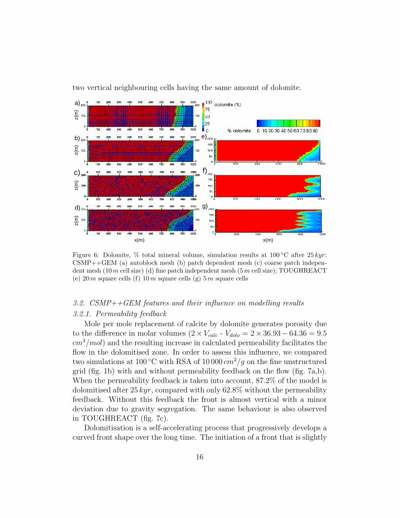
two vertical neighbouring cells having the same amount of dolomite.

a)

b)

c)

d)

f)

g)

x(m) x(m)

z(m

)z(

m)

z(m

)z(

m)

e)

Figure 6: Dolomite, % total mineral volume, simulation results at 100 C after 25 kyr:CSMP++GEM (a) autoblock mesh (b) patch dependent mesh (c) coarse patch indepen-dent mesh (10m cell size) (d) fine patch independent mesh (5m cell size); TOUGHREACT(e) 20m square cells (f) 10m square cells (g) 5m square cells

3.2. CSMP++GEM features and their influence on modelling results

3.2.1. Permeability feedback

Mole per mole replacement of calcite by dolomite generates porosity dueto the difference in molar volumes (2×Vcalc - Vdolo = 2× 36.93− 64.36 = 9.5cm3/mol) and the resulting increase in calculated permeability facilitates theflow in the dolomitised zone. In order to assess this influence, we comparedtwo simulations at 100 C with RSA of 10 000 cm2/g on the fine unstructuredgrid (fig. 1b) with and without permeability feedback on the flow (fig. 7a,b).When the permeability feedback is taken into account, 87.2% of the model isdolomitised after 25 kyr, compared with only 62.8% without the permeabilityfeedback. Without this feedback the front is almost vertical with a minordeviation due to gravity segregation. The same behaviour is also observedin TOUGHREACT (fig. 7c).

Dolomitisation is a self-accelerating process that progressively develops acurved front shape over the long time. The initiation of a front that is slightly

16

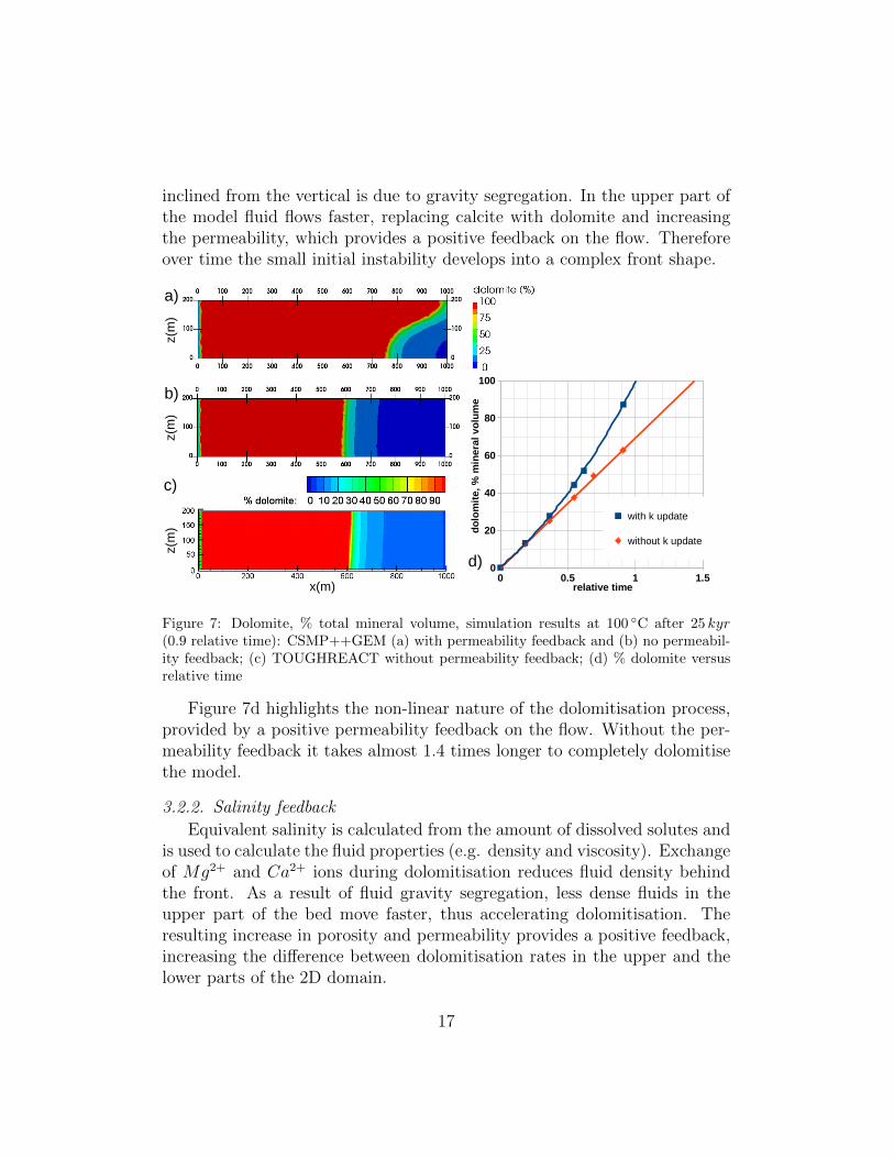
inclined from the vertical is due to gravity segregation. In the upper part ofthe model fluid flows faster, replacing calcite with dolomite and increasingthe permeability, which provides a positive feedback on the flow. Thereforeover time the small initial instability develops into a complex front shape.

a)

b)

z(m

)z(

m)

z(m

)

c)

x(m)0 0.5 1 1.5

0

20

40

60

80

100

with k update Polynomial (with k update)

without k update Linear (without k update)

relative time

do

lom

ite,

% m

iner

al v

olu

me

0 0.5 1 1.50

20

40

60

80

100

with k update Polynomial (with k update)

without k update Linear (without k update)

relative time

do

lom

ite,

% m

iner

al v

olu

me

0 0.5 1 1.50

20

40

60

80

100

with k update Polynomial (with k update)

without k update Linear (without k update)

relative time

do

lom

ite,

% m

iner

al v

olu

me

d)

Figure 7: Dolomite, % total mineral volume, simulation results at 100 C after 25 kyr(0.9 relative time): CSMP++GEM (a) with permeability feedback and (b) no permeabil-ity feedback; (c) TOUGHREACT without permeability feedback; (d) % dolomite versusrelative time

Figure 7d highlights the non-linear nature of the dolomitisation process,provided by a positive permeability feedback on the flow. Without the per-meability feedback it takes almost 1.4 times longer to completely dolomitisethe model.

3.2.2. Salinity feedback

Equivalent salinity is calculated from the amount of dissolved solutes andis used to calculate the fluid properties (e.g. density and viscosity). Exchangeof Mg2+ and Ca2+ ions during dolomitisation reduces fluid density behindthe front. As a result of fluid gravity segregation, less dense fluids in theupper part of the bed move faster, thus accelerating dolomitisation. Theresulting increase in porosity and permeability provides a positive feedback,increasing the difference between dolomitisation rates in the upper and thelower parts of the 2D domain.

17

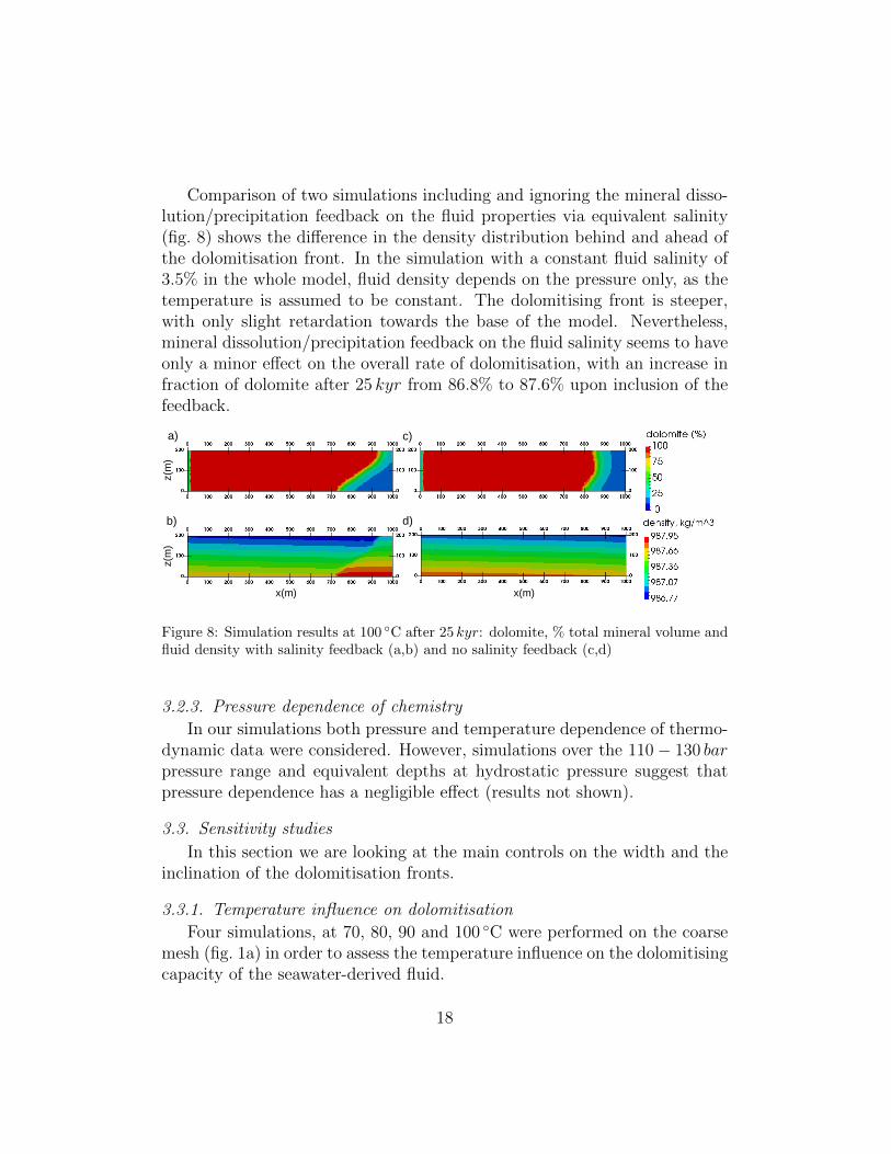
Comparison of two simulations including and ignoring the mineral disso-lution/precipitation feedback on the fluid properties via equivalent salinity(fig. 8) shows the difference in the density distribution behind and ahead ofthe dolomitisation front. In the simulation with a constant fluid salinity of3.5% in the whole model, fluid density depends on the pressure only, as thetemperature is assumed to be constant. The dolomitising front is steeper,with only slight retardation towards the base of the model. Nevertheless,mineral dissolution/precipitation feedback on the fluid salinity seems to haveonly a minor effect on the overall rate of dolomitisation, with an increase infraction of dolomite after 25 kyr from 86.8% to 87.6% upon inclusion of thefeedback.

a)

b) d)

c)

x(m) x(m)

z(m

)z(

m)

Figure 8: Simulation results at 100 C after 25 kyr: dolomite, % total mineral volume andfluid density with salinity feedback (a,b) and no salinity feedback (c,d)

3.2.3. Pressure dependence of chemistry

In our simulations both pressure and temperature dependence of thermo-dynamic data were considered. However, simulations over the 110 − 130 barpressure range and equivalent depths at hydrostatic pressure suggest thatpressure dependence has a negligible effect (results not shown).

3.3. Sensitivity studies

In this section we are looking at the main controls on the width and theinclination of the dolomitisation fronts.

3.3.1. Temperature influence on dolomitisation

Four simulations, at 70, 80, 90 and 100 C were performed on the coarsemesh (fig. 1a) in order to assess the temperature influence on the dolomitisingcapacity of the seawater-derived fluid.

18

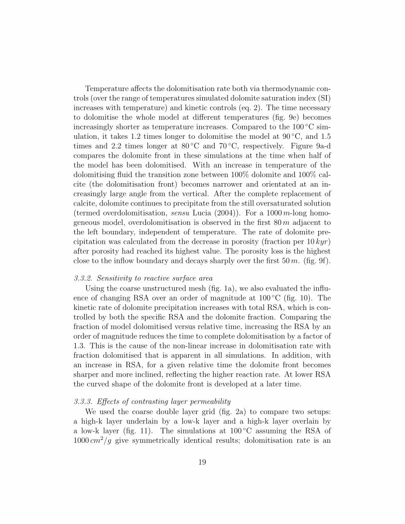
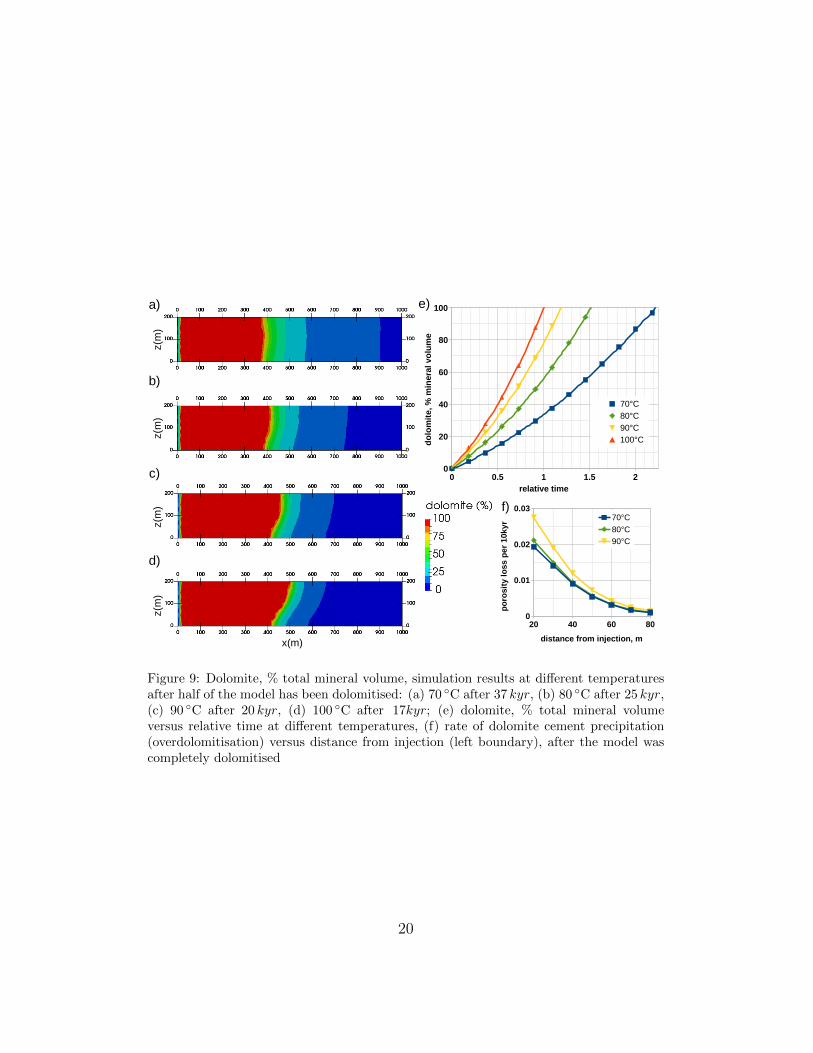
Temperature affects the dolomitisation rate both via thermodynamic con-trols (over the range of temperatures simulated dolomite saturation index (SI)increases with temperature) and kinetic controls (eq. 2). The time necessaryto dolomitise the whole model at different temperatures (fig. 9e) becomesincreasingly shorter as temperature increases. Compared to the 100 C sim-ulation, it takes 1.2 times longer to dolomitise the model at 90 C, and 1.5times and 2.2 times longer at 80 C and 70 C, respectively. Figure 9a-dcompares the dolomite front in these simulations at the time when half ofthe model has been dolomitised. With an increase in temperature of thedolomitising fluid the transition zone between 100% dolomite and 100% cal-cite (the dolomitisation front) becomes narrower and orientated at an in-creasingly large angle from the vertical. After the complete replacement ofcalcite, dolomite continues to precipitate from the still oversaturated solution(termed overdolomitisation, sensu Lucia (2004)). For a 1000m-long homo-geneous model, overdolomitisation is observed in the first 80m adjacent tothe left boundary, independent of temperature. The rate of dolomite pre-cipitation was calculated from the decrease in porosity (fraction per 10 kyr)after porosity had reached its highest value. The porosity loss is the highestclose to the inflow boundary and decays sharply over the first 50m. (fig. 9f).

3.3.2. Sensitivity to reactive surface area

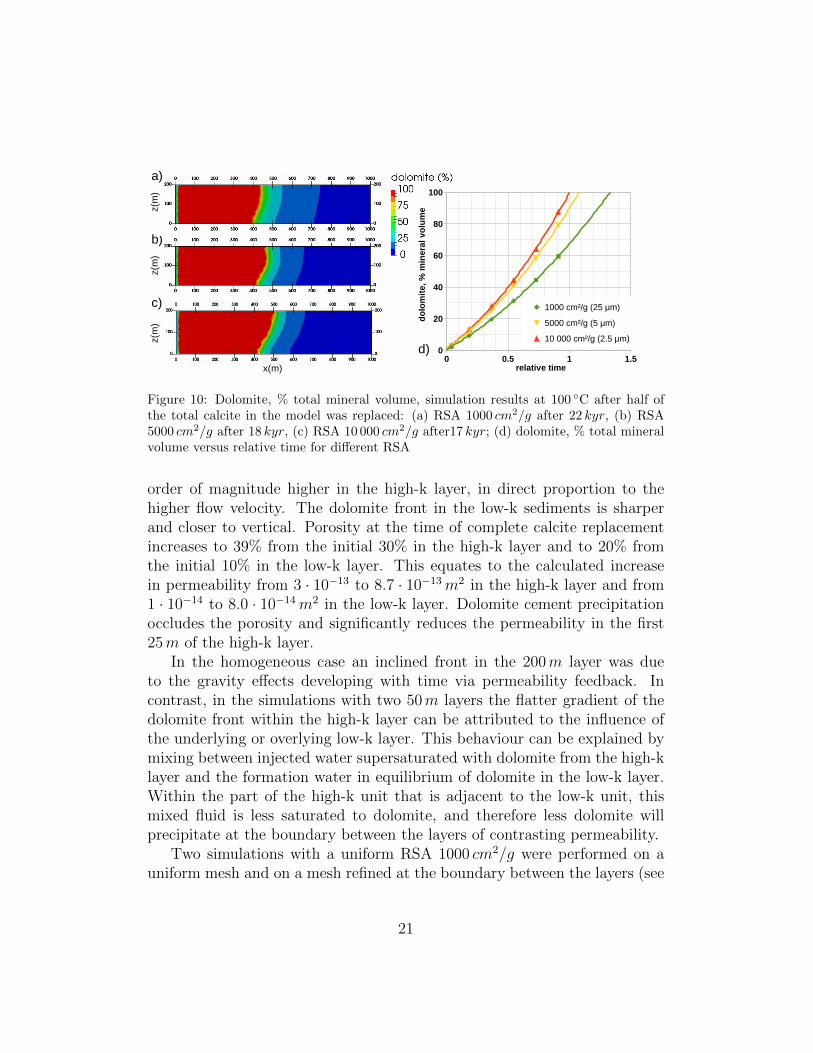
Using the coarse unstructured mesh (fig. 1a), we also evaluated the influ-ence of changing RSA over an order of magnitude at 100 C (fig. 10). Thekinetic rate of dolomite precipitation increases with total RSA, which is con-trolled by both the specific RSA and the dolomite fraction. Comparing thefraction of model dolomitised versus relative time, increasing the RSA by anorder of magnitude reduces the time to complete dolomitisation by a factor of1.3. This is the cause of the non-linear increase in dolomitisation rate withfraction dolomitised that is apparent in all simulations. In addition, withan increase in RSA, for a given relative time the dolomite front becomessharper and more inclined, reflecting the higher reaction rate. At lower RSAthe curved shape of the dolomite front is developed at a later time.

3.3.3. Effects of contrasting layer permeability

We used the coarse double layer grid (fig. 2a) to compare two setups:a high-k layer underlain by a low-k layer and a high-k layer overlain bya low-k layer (fig. 11). The simulations at 100 C assuming the RSA of1000 cm2/g give symmetrically identical results; dolomitisation rate is an

19

20 40 60 800

0.01

0.02

0.0370°C

80°C

90°C

distance from injection, m

po

rosi

ty l

oss

per

10k

yr

a)

b)

c)

d)

x(m)

z(m

)z(

m)

z(m

)z(

m)

0 0.5 1 1.5 20

20

40

60

80

100

70°C Polynomial (70°C)

80°C Polynomial (80°C)

90°C Polynomial (90°C)

100°C Polynomial (100°C)

relative time

do

lom

ite,

% m

iner

al v

olu

me

f)

e)

0 0.5 1 1.5 20

20

40

60

80

100

70°C Polynomial (70°C)

80°C Polynomial (80°C)

90°C Polynomial (90°C)

100°C Polynomial (100°C)

relative time

do

lom

ite,

% m

iner

al v

olu

me

0 0.5 1 1.5 20

20

40

60

80

100

70°C Polynomial (70°C)

80°C Polynomial (80°C)

90°C Polynomial (90°C)

100°C Polynomial (100°C)

relative time

do

lom

ite,

% m

iner

al v

olu

me

Figure 9: Dolomite, % total mineral volume, simulation results at different temperaturesafter half of the model has been dolomitised: (a) 70 C after 37 kyr, (b) 80 C after 25 kyr,(c) 90 C after 20 kyr, (d) 100 C after 17kyr; (e) dolomite, % total mineral volumeversus relative time at different temperatures, (f) rate of dolomite cement precipitation(overdolomitisation) versus distance from injection (left boundary), after the model wascompletely dolomitised

20

0 0.5 1 1.50

20

40

60

80

100

1000 cm²/g (25 μm) Polynomial (1000 cm²/g (25 μm))

5000 cm²/g (5 μm) Polynomial (5000 cm²/g (5 μm))

10 000 cm²/g (2.5 μm) Polynomial (10 000 cm²/g (2.5 μm))

relative time

do

lom

ite,

% m

iner

al v

olu

me

b)

a)

c)

x(m)

z(m

)z(

m)

z(m

)

0 0.5 1 1.50

20

40

60

80

100

1000 cm²/g (25 μm) Polynomial (1000 cm²/g (25 μm))

5000 cm²/g (5 μm) Polynomial (5000 cm²/g (5 μm))

10 000 cm²/g (2.5 μm) Polynomial (10 000 cm²/g (2.5 μm))

relative time

do

lom

ite,

% m

iner

al v

olu

me

0 0.5 1 1.50

20

40

60

80

100

1000 cm²/g (25 μm) Polynomial (1000 cm²/g (25 μm))

5000 cm²/g (5 μm) Polynomial (5000 cm²/g (5 μm))

10 000 cm²/g (2.5 μm) Polynomial (10 000 cm²/g (2.5 μm))

relative time

do

lom

ite,

% m

iner

al v

olu

me

d)

Figure 10: Dolomite, % total mineral volume, simulation results at 100 C after half ofthe total calcite in the model was replaced: (a) RSA 1000 cm2/g after 22 kyr, (b) RSA5000 cm2/g after 18 kyr, (c) RSA 10 000 cm2/g after17 kyr; (d) dolomite, % total mineralvolume versus relative time for different RSA

order of magnitude higher in the high-k layer, in direct proportion to thehigher flow velocity. The dolomite front in the low-k sediments is sharperand closer to vertical. Porosity at the time of complete calcite replacementincreases to 39% from the initial 30% in the high-k layer and to 20% fromthe initial 10% in the low-k layer. This equates to the calculated increasein permeability from 3 · 10−13 to 8.7 · 10−13m2 in the high-k layer and from1 · 10−14 to 8.0 · 10−14m2 in the low-k layer. Dolomite cement precipitationoccludes the porosity and significantly reduces the permeability in the first25m of the high-k layer.

In the homogeneous case an inclined front in the 200m layer was dueto the gravity effects developing with time via permeability feedback. Incontrast, in the simulations with two 50m layers the flatter gradient of thedolomite front within the high-k layer can be attributed to the influence ofthe underlying or overlying low-k layer. This behaviour can be explained bymixing between injected water supersaturated with dolomite from the high-klayer and the formation water in equilibrium of dolomite in the low-k layer.Within the part of the high-k unit that is adjacent to the low-k unit, thismixed fluid is less saturated to dolomite, and therefore less dolomite willprecipitate at the boundary between the layers of contrasting permeability.

Two simulations with a uniform RSA 1000 cm2/g were performed on auniform mesh and on a mesh refined at the boundary between the layers (see

21

c)

b) d)

a)

x(m) x(m)

z(m

)z(

m) high-k

high-k high-k

high-k

low-k

low-klow-k

low-k

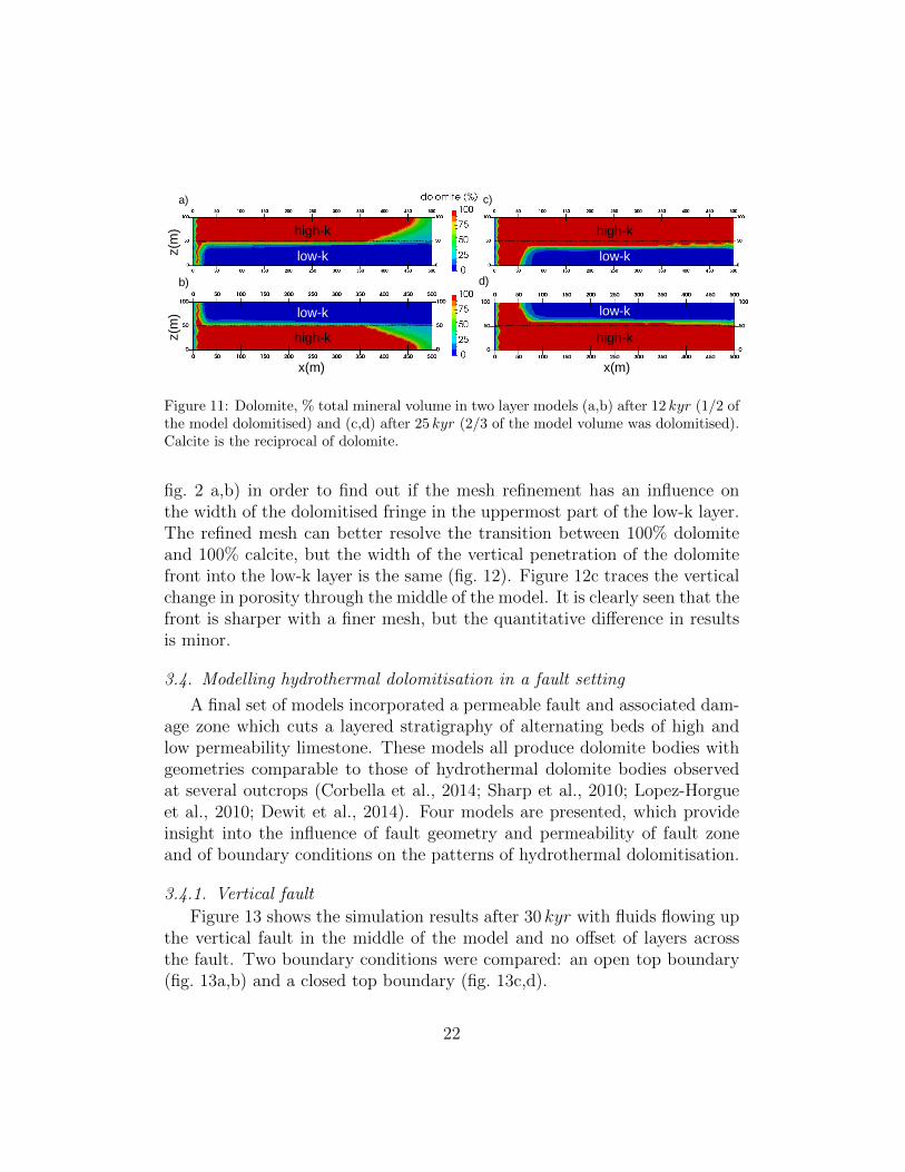
Figure 11: Dolomite, % total mineral volume in two layer models (a,b) after 12 kyr (1/2 ofthe model dolomitised) and (c,d) after 25 kyr (2/3 of the model volume was dolomitised).Calcite is the reciprocal of dolomite.

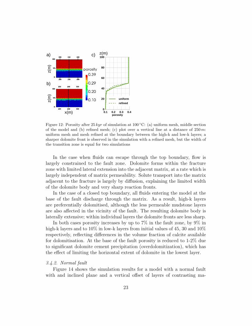
fig. 2 a,b) in order to find out if the mesh refinement has an influence onthe width of the dolomitised fringe in the uppermost part of the low-k layer.The refined mesh can better resolve the transition between 100% dolomiteand 100% calcite, but the width of the vertical penetration of the dolomitefront into the low-k layer is the same (fig. 12). Figure 12c traces the verticalchange in porosity through the middle of the model. It is clearly seen that thefront is sharper with a finer mesh, but the quantitative difference in resultsis minor.

3.4. Modelling hydrothermal dolomitisation in a fault setting

A final set of models incorporated a permeable fault and associated dam-age zone which cuts a layered stratigraphy of alternating beds of high andlow permeability limestone. These models all produce dolomite bodies withgeometries comparable to those of hydrothermal dolomite bodies observedat several outcrops (Corbella et al., 2014; Sharp et al., 2010; Lopez-Horgueet al., 2010; Dewit et al., 2014). Four models are presented, which provideinsight into the influence of fault geometry and permeability of fault zoneand of boundary conditions on the patterns of hydrothermal dolomitisation.

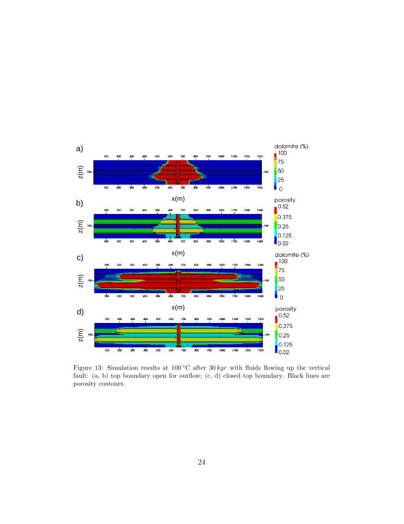
3.4.1. Vertical fault

Figure 13 shows the simulation results after 30 kyr with fluids flowing upthe vertical fault in the middle of the model and no offset of layers acrossthe fault. Two boundary conditions were compared: an open top boundary(fig. 13a,b) and a closed top boundary (fig. 13c,d).

22

a)

b)

0.1 0.2 0.3 0.40

20

40

60

80

100

porosity

porosity

c) z(m)

x(m)

z(m

)z(

m)

0.1 0.2 0.3 0.40

20

40

60

80

100

porosity

porosity

uniform

refined

Figure 12: Porosity after 25 kyr of simulation at 100 C: (a) uniform mesh, middle sectionof the model and (b) refined mesh; (c) plot over a vertical line at a distance of 250m:uniform mesh and mesh refined at the boundary between the high-k and low-k layers; asharper dolomite front is observed in the simulation with a refined mesh, but the width ofthe transition zone is equal for two simulations

In the case when fluids can escape through the top boundary, flow islargely constrained to the fault zone. Dolomite forms within the fracturezone with limited lateral extension into the adjacent matrix, at a rate which islargely independent of matrix permeability. Solute transport into the matrixadjacent to the fracture is largely by diffusion, explaining the limited widthof the dolomite body and very sharp reaction fronts.

In the case of a closed top boundary, all fluids entering the model at thebase of the fault discharge through the matrix. As a result, high-k layersare preferentially dolomitised, although the less permeable mudstone layersare also affected in the vicinity of the fault. The resulting dolomite body islaterally extensive; within individual layers the dolomite fronts are less sharp.

In both cases porosity increases by up to 7% in the fault zone, by 9% inhigh-k layers and to 10% in low-k layers from initial values of 45, 30 and 10%respectively, reflecting differences in the volume fraction of calcite availablefor dolomitisation. At the base of the fault porosity is reduced to 1-2% dueto significant dolomite cement precipitation (overdolomitization), which hasthe effect of limiting the horizontal extent of dolomite in the lowest layer.

3.4.2. Normal fault

Figure 14 shows the simulation results for a model with a normal faultwith and inclined plane and a vertical offset of layers of contrasting ma-

23

a)

c)

d)

b)

x(m)

x(m)

x(m)

z(m

)z(

m)

z(m

)z(

m)

Figure 13: Simulation results at 100 C after 30 kyr with fluids flowing up the verticalfault: (a, b) top boundary open for outflow; (c, d) closed top boundary. Black lines areporosity contours.

24

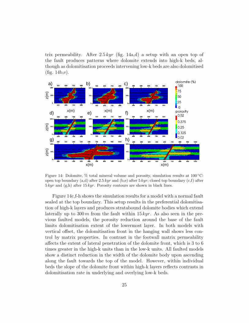
trix permeability. After 2.5 kyr (fig. 14a,d) a setup with an open top ofthe fault produces patterns where dolomite extends into high-k beds, al-though as dolomitisation proceeds intervening low-k beds are also dolomitised(fig. 14b,e).

x(m) x(m)

x(m)x(m)x(m)

z(m

)z(

m)

z(m

)

a) b) c)

f)

h)g)

d) e)

Figure 14: Dolomite, % total mineral volume and porosity, simulation results at 100 C:open top boundary (a,d) after 2.5 kyr and (b,e) after 5 kyr; closed top boundary (c,f) after5 kyr and (g,h) after 15 kyr. Porosity contours are shown in black lines.

Figure 14c,f-h shows the simulation results for a model with a normal faultsealed at the top boundary. This setup results in the preferential dolomitisa-tion of high-k layers and produces stratabound dolomite bodies which extendlaterally up to 300m from the fault within 15 kyr. As also seen in the pre-vious faulted models, the porosity reduction around the base of the faultlimits dolomitisation extent of the lowermost layer. In both models withvertical offset, the dolomitisation front in the hanging wall shows less con-trol by matrix properties. In contrast in the footwall matrix permeabilityaffects the extent of lateral penetration of the dolomite front, which is 3 to 6times greater in the high-k units than in the low-k units. All faulted modelsshow a distinct reduction in the width of the dolomite body upon ascendingalong the fault towards the top of the model. However, within individualbeds the slope of the dolomite front within high-k layers reflects contrasts indolomitisation rate in underlying and overlying low-k beds.

25

4. Discussion

4.1. Effects of numerical solution procedure on modelling results

RTM simulations can provide an understanding of the operation of indi-vidual controls on complex coupled systems controlled by fluid flow, solutetransport and water-rock reactions in a manner that is impossible to extractfrom natural systems. However, while in our simple homogeneous models wetried to decouple different model features, there always remains an interplayof various factors. For example, temperature of the dolomitising fluid plays acrucial role in controlling reaction rate, but its influence on buoyancy meansthat it is also strongly connected to the influence of gravity. In thin beds,gravity is less pronounced than in thicker beds. Both reaction rate and grav-itational segregation affect the front shape. Our simulations illustrate why itis important to understand the fundamental processes governing behavioursof a simple modelled system before we can meaningfully apply the results ofsimulations to better understand natural systems.

The synergies between factors that influence the dolomitisation processare fundamentally dependent upon the feedback on the fluid flow from thepermeability increase. This results in important non-linearities in the de-velopment of dolomitisation. However, the assumed relationship betweenmodelled changes in porosity and the effective permeability is key.

An important application of simple homogeneous models is to understandthe issues tied to the numerical solution procedure. The reactive transportsystem controlling even a simple replacement of calcite by dolomite is so com-plex that an analytical solution is not possible. Numerical solution is neverexact and direct comparison of RTM simulations performed with differentcodes is challenging (Yapparova et al., 2017).

Our CSMP++GEM simulations generate consistent results and show thatour code is applicable in practice. In contrast, our TOUGHREACT sim-ulations with increasing mesh refinement show a diverging behaviour andincreasing numerical instabilities.

Evaluation of the effect of differently structured meshes shows that weget quantitatively comparable results for different types of meshes, but thereare small differences that are directly related to the mesh type. Structuredcorner-grid meshes are widely used in codes including TOUGHREACT (Xuet al., 2004) and our comparison here has shown that they cannot resolvesome of the fine features.

26

Unstructured grids offer a number of important advantages, most im-portantly mesh refinement and adaptivity to non-linear geometrical featuresreflecting depositional facies, deformation features (i.e. faults, fractures) andprior diagenesis. Unstructured grids are already being used in the new gen-eration reactive transport codes like PFLOTRAN (Lichtner et al., 2017).

A key challenge facing geologists with limited direct experience of process-based modelling is to understand which features of published simulationshave broad applicability, and which originate from numerical procedures andmodel set-up. This can be exemplified by comparison between results fromour double layer models and those of facies dependent dolomitisation in EarlyCretaceous rocks at Benicassim, Maestrat Basin, eastern Spain.

RTM simulations by Corbella et al. (2014) show preferential dolomitisa-tion of the more porous and permeable packstone-grainstone layers, whichover a long period of time also affects interbedded less porous and permeablemudstone-wackestone layers to produce massive dolomite bodies. Similarbehaviour is observed in our models, although in simulations from Corbellaet al. (2014) dolomitisation is much slower, despite using the same reactionkinetics. We attribute this difference to the incorporation in both our modeland in TOUGHREACT of a feedback between evolving porosity and per-meability, missing from the software used by Corbella et al. (2014). Withthis permeability update disabled, our models predict dolomitisation occur-ring more slowly and at a constant rate, independent of dolomite abundance.The increase in permeability during replacement phase makes dolomitisa-tion a self-accelerating process: dolomitisation driving an increasing focus ofreactive fluids in the more permeable beds and enhancing the permeabilitycontrast between the beds. More rapid dolomitisation in the more permeableunits also produces sharper dolomite fronts.

A further difference of some significance is that Corbella et al. (2014)assume that both calcite and dolomite are kinetically controlled minerals.As a result, in their simulations calcite dissolution and dolomite precipita-tion do not occur simultaneously: calcite is dissolved preferentially in thehigh-permeability beds whereas dolomite is mostly precipitated in the low-permeability beds (the opposite to that observed in the field). The apparentdecoupling of the two reactions also does not accord with the chemical sys-tem that we model, which suggests that precipitation of dolomite is drivinglocal calcite dissolution and that the dolomite growth rate is so slow thatcalcite effectively remains in local equilibrium with the fluid.

27

4.2. Fault-controlled dolomitisation and HTD geobodiesOur simulations of the faulted systems suggest that the style of dolomi-

tisation is governed mainly by the presence or absence of a top seal. Whena zone of low permeability prevents the vertical escape of diagenetic fluidsflowing upward in a fault zone, the fringes of dolomite extend laterally intomore permeable beds within the surrounding host rock. However, when thepermeable fault conduit cross-cuts depositional stratigraphy and connectsthe reservoir of fluids to a sink (such as the sea floor), advection is largelyconstrained within the plane of the fault and the associated damage zone.Since, in this case, solute exchange with the rock matrix occurs largely by dif-fusion, dolomitisation only extends over short distances from the fault zone,forming a massive body with sharp diagenetic fronts.

Compared to the model with a displacive normal fault, a vertical faultwithout layer displacement produces a symmetrical dolomite body. Daviesand Smith (2006) suggest a normal fault would result in a preferential dolomi-tisation of the hanging-wall site, due to the thermal gradient and fluids mov-ing up due to gravity segregation. This accords with our models that showpervasive dolomitisation on the hanging-wall side and the development ofstratabound dolomite bodies on the foot-wall side (fig. 14g).

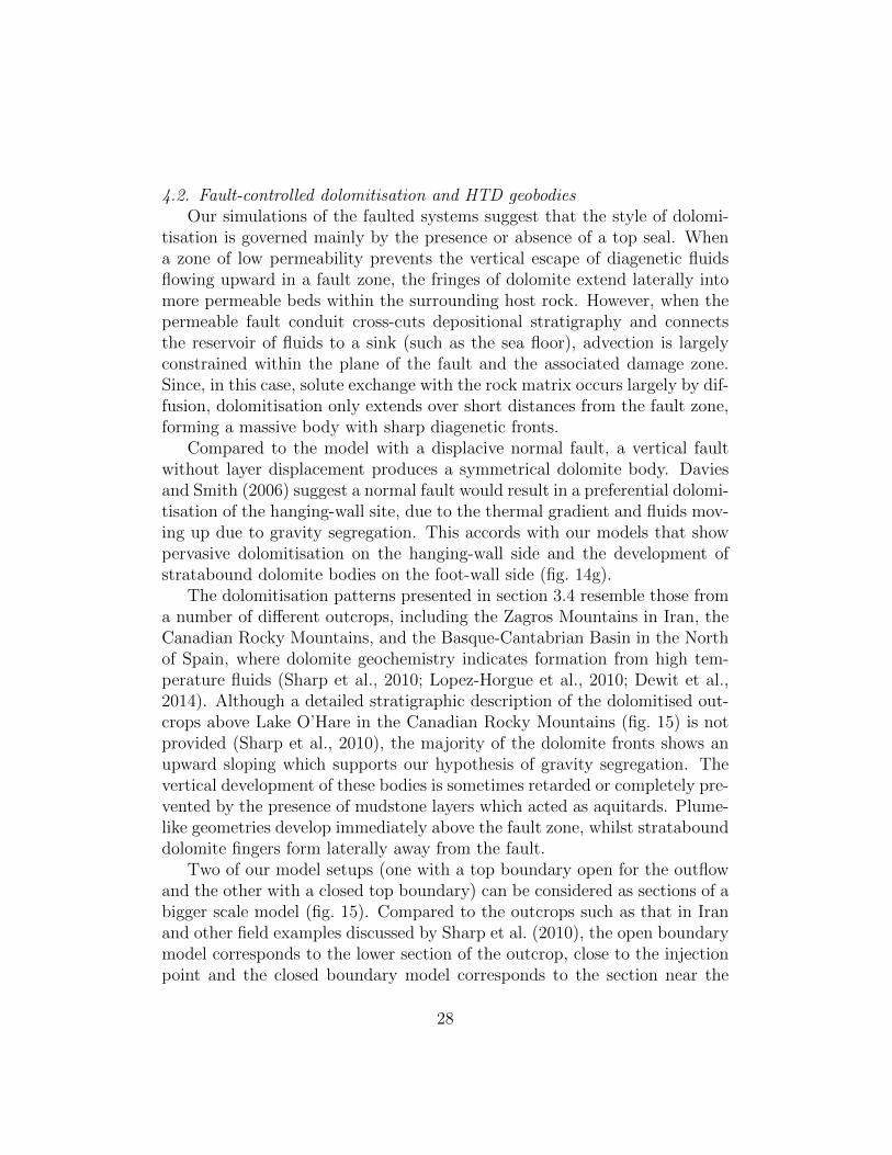
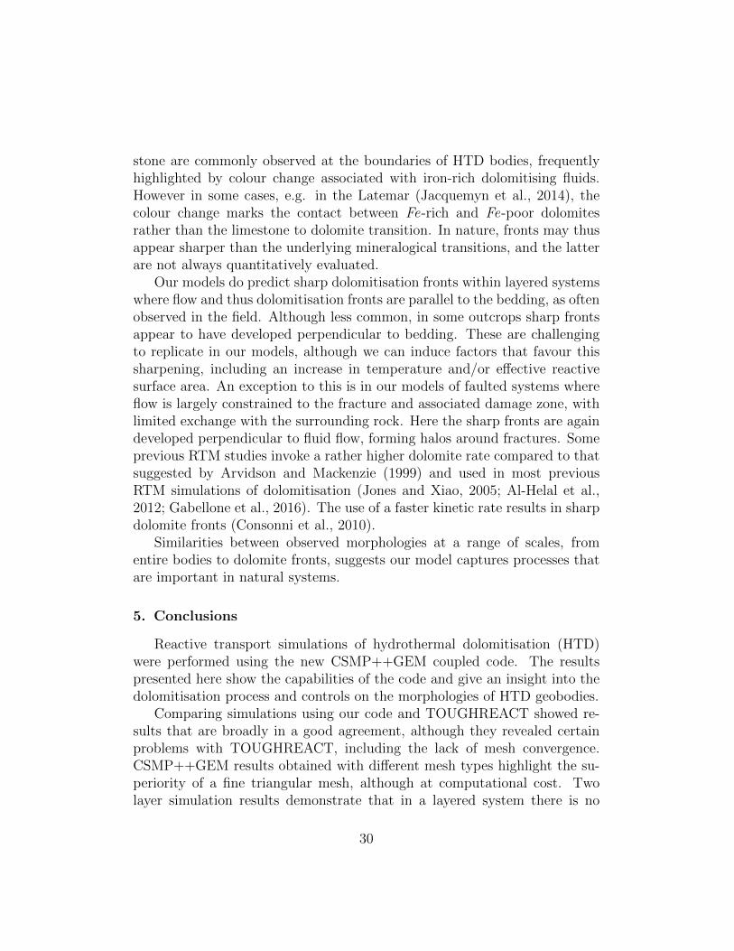
The dolomitisation patterns presented in section 3.4 resemble those froma number of different outcrops, including the Zagros Mountains in Iran, theCanadian Rocky Mountains, and the Basque-Cantabrian Basin in the Northof Spain, where dolomite geochemistry indicates formation from high tem-perature fluids (Sharp et al., 2010; Lopez-Horgue et al., 2010; Dewit et al.,2014). Although a detailed stratigraphic description of the dolomitised out-crops above Lake O’Hare in the Canadian Rocky Mountains (fig. 15) is notprovided (Sharp et al., 2010), the majority of the dolomite fronts shows anupward sloping which supports our hypothesis of gravity segregation. Thevertical development of these bodies is sometimes retarded or completely pre-vented by the presence of mudstone layers which acted as aquitards. Plume-like geometries develop immediately above the fault zone, whilst stratabounddolomite fingers form laterally away from the fault.

Two of our model setups (one with a top boundary open for the outflowand the other with a closed top boundary) can be considered as sections of abigger scale model (fig. 15). Compared to the outcrops such as that in Iranand other field examples discussed by Sharp et al. (2010), the open boundarymodel corresponds to the lower section of the outcrop, close to the injectionpoint and the closed boundary model corresponds to the section near the

28

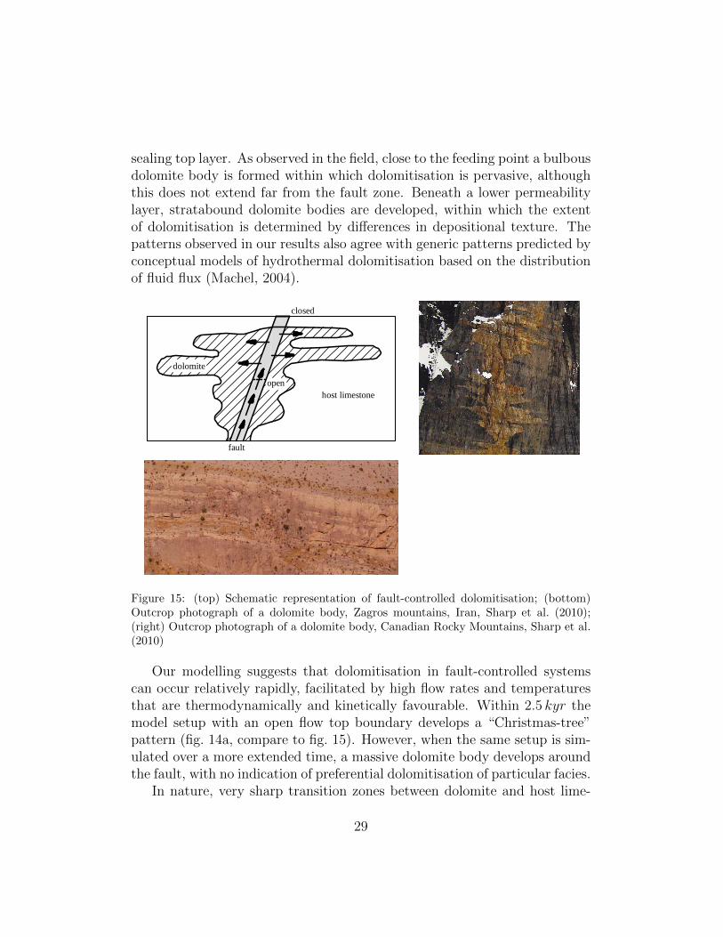
sealing top layer. As observed in the field, close to the feeding point a bulbousdolomite body is formed within which dolomitisation is pervasive, althoughthis does not extend far from the fault zone. Beneath a lower permeabilitylayer, stratabound dolomite bodies are developed, within which the extentof dolomitisation is determined by differences in depositional texture. Thepatterns observed in our results also agree with generic patterns predicted byconceptual models of hydrothermal dolomitisation based on the distributionof fluid flux (Machel, 2004).

fault

dolomite

closed

openhost limestone

Figure 15: (top) Schematic representation of fault-controlled dolomitisation; (bottom)Outcrop photograph of a dolomite body, Zagros mountains, Iran, Sharp et al. (2010);(right) Outcrop photograph of a dolomite body, Canadian Rocky Mountains, Sharp et al.(2010)

Our modelling suggests that dolomitisation in fault-controlled systemscan occur relatively rapidly, facilitated by high flow rates and temperaturesthat are thermodynamically and kinetically favourable. Within 2.5 kyr themodel setup with an open flow top boundary develops a “Christmas-tree”pattern (fig. 14a, compare to fig. 15). However, when the same setup is sim-ulated over a more extended time, a massive dolomite body develops aroundthe fault, with no indication of preferential dolomitisation of particular facies.

In nature, very sharp transition zones between dolomite and host lime-

29

stone are commonly observed at the boundaries of HTD bodies, frequentlyhighlighted by colour change associated with iron-rich dolomitising fluids.However in some cases, e.g. in the Latemar (Jacquemyn et al., 2014), thecolour change marks the contact between Fe-rich and Fe-poor dolomitesrather than the limestone to dolomite transition. In nature, fronts may thusappear sharper than the underlying mineralogical transitions, and the latterare not always quantitatively evaluated.

Our models do predict sharp dolomitisation fronts within layered systemswhere flow and thus dolomitisation fronts are parallel to the bedding, as oftenobserved in the field. Although less common, in some outcrops sharp frontsappear to have developed perpendicular to bedding. These are challengingto replicate in our models, although we can induce factors that favour thissharpening, including an increase in temperature and/or effective reactivesurface area. An exception to this is in our models of faulted systems whereflow is largely constrained to the fracture and associated damage zone, withlimited exchange with the surrounding rock. Here the sharp fronts are againdeveloped perpendicular to fluid flow, forming halos around fractures. Someprevious RTM studies invoke a rather higher dolomite rate compared to thatsuggested by Arvidson and Mackenzie (1999) and used in most previousRTM simulations of dolomitisation (Jones and Xiao, 2005; Al-Helal et al.,2012; Gabellone et al., 2016). The use of a faster kinetic rate results in sharpdolomite fronts (Consonni et al., 2010).

Similarities between observed morphologies at a range of scales, fromentire bodies to dolomite fronts, suggests our model captures processes thatare important in natural systems.

5. Conclusions

Reactive transport simulations of hydrothermal dolomitisation (HTD)were performed using the new CSMP++GEM coupled code. The resultspresented here show the capabilities of the code and give an insight into thedolomitisation process and controls on the morphologies of HTD geobodies.

Comparing simulations using our code and TOUGHREACT showed re-sults that are broadly in a good agreement, although they revealed certainproblems with TOUGHREACT, including the lack of mesh convergence.CSMP++GEM results obtained with different mesh types highlight the su-periority of a fine triangular mesh, although at computational cost. Twolayer simulation results demonstrate that in a layered system there is no

30

need for mesh refinement along the boundary between the layers of differentrock types.

Simple models with homogeneous rock properties allowed us to study thesynergistic effect of gravity and permeability influence on the flow field indetail and to find a reasonable explanation for the self-accelerating nature ofthe dolomitisation process and the inclined shape of the dolomitisation front.

In a 200m-thick homogeneous unit, gravity segregation initiates the frontinstability and via the permeability feedback promotes faster dolomitisationin the upper part of the model. However, with two 50m thick beds of con-trasting rock properties, the lower permeability bed has a crucial impact onthe shape of the dolomitisation front in the higher permeability bed.

Although the feedback of chemical reactions on fluid salinity and thepressure dependence of thermodynamic data have a minor influence on therate of dolomitisation progress and the shape of dolomitisation front, in amore complex scenario (concentrated seawater, higher pressure differences)these effects might play a more significant role.

With an increase in fluid temperature and reactive surface area the dolomi-tisation rate increases and the dolomite fronts become sharper (decreasingwidth of the transition zone from calcite to dolomite). Likewise, the rateof primary dolomite cement precipitation after complete calcite replacementincreases with temperature.

Simulations of fault-controlled hydrothermal dolomitisation generate dolomitegeobodies comparable in morphology to natural examples documented at out-crops, and underline the importance of permeability structure. In particular,our results show that stratabound dolomites tend to form in HTD systemswhen the fluids sourced from a fault encounter a low permeability barrier atthe top of the fault. On the other hand, more massive dolomite bodies tendto form when the fault top is not sealed. The geometry of the fault has aneffect on the dolomitisation trends, producing symmetrical bodies when it isvertical, or otherwise preferential alteration of the hanging-wall side when itis inclined and with layer displaced.

Our reactive transport simulations are currently limited to 2D due to thehigh computational cost, and thus may lack features which could emergefrom simulation of HTD in 3D. There is ongoing development of the parallelversion of CSMP++GEM that will increase the utility of our code and allowmore complex reactive transport simulations.

31

Acknowledgements

We thank BG Group, Chevron, Petrobras, Saudi Aramco and Winter-shall for sponsorship of the University of Bristol ITF (Industry TechnologyFacilitator) project IRT-MODE.

Authors are grateful to James Patterson for creating the ANSYS meshes.We appreciated productive discussions with Wilfred Pfingsten and GeorgKosakowski and their valuable insight into the TOUGHREACT comparisonproblem. Authors thank Zarema Amirova for drawing the fault-controlleddolomitisation sketch. We would like to thank the two anonymous reviewersfor their comments that helped focus the paper and increase its readability.

Agar, S. M., Geiger, S., 2015. Fundamental controls on fluid flow in car-bonates: current workflows to emerging technologies. Geological Society,London, Special Publications 406 (1), 1–59.

Al-Helal, A. B., Whitaker, F. F., Xiao, Y., 2012. Reactive transport mod-eling of brine reflux: dolomitisation, anhydrite precipitation and porosityevolution. Journal of Sedimentary Research 82, 196–215.

Arvidson, R., Mackenzie, F., 1999. The dolomite problem; control of precip-itation kinetics by temperature and saturation state. Am. J. Sci. 299(4),257–288.

Blanc, P., Lassin, A., Piantone, P., Azaroual, M., Jacquemet, N., Fabbri, A.,Gaucher, E., 2012. Thermoddem: A geochemical database focused on lowtemperature water/rock interactions and waste materials. Appl. Geochem.27(10), 2107–2116.

Consonni, A., Frixa, A., Maragliulo, C., 2016. Hydrothermal dolomitization:simulation by reaction transport modelling. Geological Society, London,Special Publications 435.

Consonni, A., Ronchi, P., Geloni, C., Battistelli, A., Grigo, D., Biagi, S.,Gherardi, F., Gianelli, G., 2010. Application of numerical modelling to acase of compaction-driven dolomitization: A Jurassic palaeohigh in the PoPlain, Italy. Sedimentology 57 (1), 209–231.

Corbella, M., Gomez-Rivas, E., Martın-Martın, J. D., Stafford, S. L., Teix-ell, A., Griera, A., Trave, A., Cardellach, E., Salas, R., 2014. Insights to

32

controls on dolomitization by means of reactive transport models appliedto the Benicassim case study (Maestrat Basin, eastern Spain). PetroleumGeoscience 20 (1), 41–54.

Davies, G., Smith, L., 2006. Structurally controlled hydrothermal dolomitereservoir facies: An overview. AAPG Bull. 90(11), 1641–1690.

de Dieuleveult, C., Erhel, J., Kern, M., 2009. A global strategy for solvingreactive transport equations. Journal of Computational Physics 228 (17),6395–6410.

Dewit, J., Foubert, A., El Desouky, H. A., Muchez, P., Hunt, D., Vanhaecke,F., Swennen, R., 2014. Characteristics, genesis and parameters control-ling the development of a large stratabound HTD body at Matienzo (Ra-males Platform, Basque-Cantabrian Basin, northern Spain). Marine andPetroleum Geology 55, 6–25.

Driesner, T., Heinrich, C. A., 2007. The system H2O-NaCl . Part I : Correla-tion formulae for phase relations in temperature – pressure – compositionspace from 0 to 1000C, 0 to 5000 bar, and 0 to 1 XNaCl. Geochimica etCosmochimica Acta 71, 4880–4901.

Frazer, M., Whitaker, F., Hollis, C., 2014. Fluid expulsion from overpres-sured basins: Implications for Pb-Zn mineralisation and dolomitisationof the East Midlands platform, northern England. Marine and PetroleumGeology 55, 68–86.

Gabellone, T., Whitaker, F., 2016. Secular variations in seawater chemistrycontrolling dolomitisation in shallow reflux systems: insights from reactivetransport modelling. Sedimentology 63, 1233–1259.

Gabellone, T., Whitaker, F., Katz, D., Griffiths, G., Sonnenfeld, M., 2016.Controls on reflux dolomitisation of epeiric-scale ramps: Insights from reac-tive transport simulations of the Mississippian Madison Formation (Mon-tana and Wyoming). Sedimentary Geology 345, 85–102.

Garcia-Fresca, B., Jones, G., Tianfu, X., 2009. The apparent stratigraphicconcordance of reflux dolomite: new insights from synsedimentary reactivetransport models. AAPG Convention, June 710, Search and DiscoveryArticle N50208, Denver,Colorado.

33

Geiger, S., Roberts, S. G., Matthai, S. K., Zoppou, C., Burri, A., 2004.Combining finite element and finite volume methods for efficient multi-phase flow simulations in highly heterogeneous ans structurally complexgeologic media. Geofluids 4, 284–299.

Helgeson, H. C., Kirkham, D. H., Flowers, D. C., 1981. Theoretical predic-tion of the thermodynamic behavior of aqueous electrolytes at high pres-sures and temperatures: Iv. calculation of activity coefficients, osmoticcoefficients, and apparent molal and standard and relative partial molalproperties to 600c and 5 kb. Am. J. Sci. 281, 1249–1516.

Jacquemyn, C., Desouky, H. E., Hunt, D., Casini, G., Swennen, R., 2014.Dolomitization of the latemar platform: Fluid flow and dolomite evolution.Marine and Petroleum Geology 55, 43–67.

Jones, G. D., Gupta, I., Sonnenthal, E., 2010. Reactive Transport Models ofStructurally Controlled Hydrothermal Dolomite: Implications for MiddleEast Carbonate Reservoirs. In: 9th Middle East Geosciences Conference,GEO 2010. Vol. 16(2). GeoArabia, pp. 194–195.

Jones, G. D., Xiao, Y., 2005. Dolomitization, anhydrite cementation, andporosity evolution in a reflux system: Insights from reactive transportmodels. AAPG Bulletin 89 (5), 577–601.

Kulik, D. A., Wagner, T., Dmytrieva, S. V., Kosakowski, G., Hingerl, F. F.,Chudnenko, K. V., Berner, U. R., 2013. GEM-Selektor geochemical model-ing package: Revised algorithm and GEMS3K numerical kernel for coupledsimulation codes. Computational Geosciences 17 (1), 1–24.

Lichtner, P. C., Hammond, G. E., Lu, C., Karra, S., Bisht, G., Andre, B.,Mills, R. T., Kumar, J., Frederick, J. M., 2017. PFLOTRAN user manual.Tech. rep., http://www.documentation.pflotran.org.

Lopez-Horgue, M. A., Iriarte, E., Schroeder, S., Fernandez-Mendiola, P. A.,Caline, B., Corneyllie, H., Fremont, J., Sudrie, M., Zerti, S., 2010. Struc-turally controlled hydrothermal dolomites in Albian carbonates of the Asonvalley, Basque Cantabrian Basin, Northern Spain. Marine and PetroleumGeology 27 (5), 1069–1092.

34

Lu, P., Cantrell, D., 2016. Reactive transport modelling of reflux dolomitiza-tion in the Arab-D reservoir, Ghawar field, Saudi Arabia. Sedimentology63, 865–892.

Lucia, J. F., 2004. Origin and petrophysics of dolostone pore space. In:Braithwaite, C., Rizzi, G., Darke, G. (Eds.), The geometry and petro-genesis of dolomite hydrocarbon reservoirs. Vol. 235. Geological Society(London) Special Publication, pp. 141–155.

Machel, H. G., 2004. Concepts and models of dolomitization, a critical reap-praisal. In: Braithwaite, C., Rizzi, G., Darke, G. (Eds.), The geometryand petrogenesis of dolomite hydrocarbon reservoirs. Vol. 235. GeologicalSociety (London) Special Publication, pp. 7–63.

Machel, H. G., Lonnee, J., 2002. Hydrothermal dolomite - A product of poordefinition and imagination. In: 75th Anniversary of CSPG Convention,June 3-7, 2002. Canadian Society of Petroleum Geologists, pp. 1–8.

Nordstrom, D., Plummer, L., Wigley, T., Wolery, T., Ball, J., Jenne, E.,Bassett, R., Crerar, D., Florence, T., Fritz, B., Hoffman, M., Holdren,G., Lafon, G., Mattigod, S., McDuff, R., Morel, F., Reddy, M., Sposito,G., Thrailkill, J., 1979. A comparison of computerized chemical models forequilibrium calculations in aqueous systems. In: Jenne, E. (Ed.), Chemicalmodeling in aqueous systems - Speciation, sorption, solubility, and kinetics.Vol. 93. American Chemical Society, Series, pp. 857–892.

Qing, H., Mountjoy, E. W., 1994. Formation of coarsely crystalline, hy-drothermal dolomite reservoirs in the Presqu’ile barrier, Western CanadaSedimentary Basin. AAPG Bulletin 78 (1), 55–77.

Sharp, I., Gillespie, P., Morsalnezhad, D., Taberner, C., Karpuz, R., VergeS,J., Horbury, A., Pickard, N., Garland, J., Hunt, D., 2010. Stratigraphic ar-chitecture and fracture-controlled dolomitization of the Cretaceous Khamiand Bangestan groups: an outcrop case study, Zagros Mountains, Iran.In: van Buchem, F. S. P., Gerdes, K., Esteban, M. (Eds.), Mesozoic andCenozoic Carbonate Systems of the Mediterranean and the Middle East:Stratigraphic and Diagenetic Reference Models. Vol. 329. Geological Soci-ety, London, Special Publications, pp. 343–396.

35

Steefel, C. I., DePaolo, D. J., Lichtner, P. C., 2005. Reactive transport mod-eling: An essential tool and a new research approach for the earth sciences.Earth and Planetary Science Letters 240 (3–4), 539–558.

Thien, B., Kulik, D., Curti, E., 2014. A unified approach to model uptakekinetics of trace elements in complex aqueous-solid solution systems. Appl.Geochem. 41, 135–150.

Thoenen, T., Hummel, W., Berner, U., E., C., 2014. The psi/nagra chemicalthermodynamic database 12/07. PSI Bericht 14-04, Paul Scherrer Institut,Villigen, Switzerland.

Whitaker, F. F., Xiao, Y., 2010. Reactive transport modeling of early burialdolomitization of carbonate platforms by geothermal convection. AAPGBulletin 94 (6), 889–917.

Wilson, A. M., Sanford, W., Whitaker, F., Smart, P., 2001. Spatial patternsof diagenesis during geothermal circulation in carbonate platforms. Am. J.Sci. 301, 727–752.

Wilson, M. E. J., Evans, M. J., Oxtoby, N. H., Nas, D. S., Donnelly, T.,Thirlwall, M., 2007. Reservoir quality, textural evolution, and origin offault-associated dolomites. AAPG Bulletin 91 (9), 1247–1272.

Xiao, Y., Jones, G., Whitaker, F., Al-Helal, A., Stafford, S., Gomez-Rivas, E.,Guidry, S., 2013. Fundamental approaches to dolomitisation and carbonatediagenesis in different hydrogeological systems and the impact on reservoirquality distribution. In: International Petroleum Technology Conference,Beijing, China. pp. 1164–1179.

Xu, T., Sonnenthal, E., Spycher, N., Pruess, K., 2004. TOUGHREACTuser’s guide: a simulation program for non-isothermal multiphase reactivegeochemical transport in variable saturated geologic media. ReportLBNL-55460. Lawrence Berkeley National Laboratory, Berkeley, CA.

Yapparova, A., Gabellone, T., Whitaker, F., Kulik, D. A., Matthai,S. K., 2017. Reactive transport modelling of dolomitisation using the newCSMP++GEM coupled code: governing equations, solution method andbenchmarking results. Transport in Porous Media 117 (3), 385–413.

36