Yale ICF Working Paper No. 03-26 November 2004

TURNING OVER TURNOVER

K.J. Martijn Cremers International Center for Finance

Yale School of Management

Jianping Mei New York University

This paper can be downloaded without charge from the

Social Science Research Network Electronic Paper Collection: http://ssrn.com/abstract=452720

Turning Over Turnover

K.J. Martijn Cremers and Jianping Mei*

November 2004

Abstract

This paper applies the methodology of Bai and Ng (2002, 2004) for decomposing large

panel data into systematic and idiosyncratic components to both returns and turnover. Combining

the methodology with a generalized-least-squares-based principal components procedure, we

demonstrate that this approach works well for both returns and turnover despite the presence of

severe heteroscedasticity and non-stationarity in turnover of individual stocks. We then test the

duo-factor model of Lo and Wang’s (2000), which is based on mutual fund separation. Our

results indicate that trading due to systematic risk in returns can account for as much as 73% of

all systematic turnover variation in the weekly time-series and 76% in the cross-section. Thus,

portfolio rebalancing due to systematic risk is a very important motive for stock trading. Finally,

we demonstrate that several commonly used turnover measures may understate the impact of

stock trading.

* International Center for Finance, Yale School of Management, 135 Prospect Street, New Haven, CT 06520, tel: (203) 436-0649, martijn.cremers@yale.edu; Department of Finance, Stern School of Business, New York University, 44 West 4th Street, New York, NY 10012-1126 and CCFR, Tel: (212) 998-0354, jmei@stern.nyu.edu. This paper originally was titled “A New Approach to the Duo-factor-model of Return and Volume”. We would like to thank Andrew Ang, KC Chan, Kalok Chan, Lewis Chan, Robert Engel, Larry Harris, Joel Hasbrouck, Anthony Lynch, Gideon Saar, Jeff Wurgler, Wei Xiong, Yexiao Xu and an anonymous referee as well as seminar participants at NYU, HKUST, Rutgers University, and the University of Southern Califonia for helpful discussions. We thank Haibo Tang for excellent research assistance. We also thank Andrew Lo and Jiang Wang, who graciously provided us with their MiniCRSP data manual.

Turning Over Turnover

Abstract

This paper applies the methodology of Bai and Ng (2002, 2004) for decomposing large

panel data into systematic and idiosyncratic components to both returns and turnover. Combining

the methodology with a generalized-least-squares-based principal components procedure, we

demonstrate that this approach works well for both returns and turnover despite the presence of

severe heteroscedasticity and non-stationarity in turnover of individual stocks. We then test the

duo-factor model of Lo and Wang’s (2000), which is based on mutual fund separation. Our

results indicate that trading due to systematic risk in returns can account for as much as 73% of

all systematic turnover variation in the weekly time-series and 76% in the cross-section. Thus,

portfolio rebalancing due to systematic risk is a very important motive for stock trading. Finally,

we demonstrate that several commonly used turnover measures may understate the impact of

stock trading.

1. Introduction

There is increasing interest in improving the understanding of turnover, given its

prominence in many behavioral finance, liquidity, and asymmetric information models.1 Lo and

Wang (LW hereafter, 2000, 2003) have developed a multi-factor model for turnover based on

asset pricing models. Their model gives rise to a decomposition of turnover into systematic and

idiosyncratic components, just like the usual return-decomposition. This model has several

interesting applications in finance.

First, the decomposition of firm-level turnover into systematic and idiosyncratic

components is useful for a large number of research questions. Most theoretical models of asset

pricing and trading volume have systematic as well as firm-specific components,2 so one needs

to have separate measurements of these components in order to provide an empirical test of these

models. So far, adjusting turnover for firm-fixed effects is typically dealt with by de-trending

total turnover (see, for example, Chen, Hong and Stein (2001)). As we argue in this paper, the

systematic-idiosyncratic decomposition could be used as an alternative and likely more effective

approach.

Furthermore, numerous studies have found common (that is, systematic) components in

liquidity (e.g. Chordia, Roll, and Subrahmanyam (1998) and Hasbrouck and Seppi (2001)). The

turnover decomposition directly measures how much trading is driven by systematic factors and

how much is due to firm-specific causes. Using turnover is a proxy for informational trading, one

can relate idiosyncratic turnover to firm-specific news and evaluate the impact of information

asymmetry on asset pricing. In this paper, we demonstrate that several commonly used turnover

measures may understate the impact of stock trading.

Also, a better understanding of turnover can help provide more powerful asset pricing tests.

LW (2003) demonstrate that one can form a unique hedging portfolio using information from

stock turnover. This provides additional tests of an asset pricing model, since the hedging

1 For theoretical models of turnover see, among others, Daniel, Hirshleifer, and Subrahmanyam (1998), Duffie,

Garleanu and Pedersen (2003), Hong and Stein (1999, 2003), Scheinkman and Xiong (2003) and Vayanos and

Wang (2003). For empirical studies see Chen, Hong, and Stein (2002), Odean (1998), Ofek and Richardson (2002),

and Mei, Scheinkman, and Xiong (2003). 2 See, for example, Llorente et al (2002) and Wang (1994).

1

portfolio return together with the market return are the two risk factors determining the cross-

section of asset returns.

Despite these interesting applications, studies of turnover have largely been limited to

portfolios or to a small number of individual stocks. This may be partly due to the difficulty of

implementing conventional multi-factor estimation procedures, which results from severe

heteroscedasticity and non-stationarity found in turnover data (see LW (2000)). However,

applying procedures developed by Bai and Ng (BN hereafter, 2000, 2004), we are able to

consistently estimate the turnover factor model and test for non-stationarity. This way, we

provide a close examination of turnover by “turning over” a large panel of individual stocks.

Our study makes a number of contributions to the turnover and factor model literature.

First, we implement BN’s methodology to decompose turnover into systematic and firm-

specific components and demonstrate that for estimating the required number of factors, the BN

(2002) statistics work well for returns, but not for raw turnover. Instead, we show the importance

of standardizing turnover by way of a modified generalized-least-squares-based procedure that is

effective and simple to implement. We also show how to use the BN (2004) method to test for

non-stationarity in both systematic as well as firm-specific turnover components. Our tests reveal

that individual stock turnover consists of a systematic component that has a time trend and an

idiosycratic component that is essentially stationary. We find that the three to five (depending on

the time period) systematic turnover factors together can capture 15.47% - 26.73% of the

variation in individual stock turnover, quite similar to the percentages of individual stock return

variation that is systematic.

Second, we provide a new test of the theoretical work by LW (2000). In particular, our

empirical study uses data from a large panel of individual stocks rather than the beta-sorted

portfolios they used. By exploiting the advantage of a large cross-section of individual stocks, we

get around the non-stationarity issue in turnover. As our empirical work shows, the number of

systematic factors in return and turnover changes dramatically when individual stocks are used

instead of beta-sorted portfolios.3

3 Berk (2000) shows a significant drop in statistical power in asset pricing tests using firm-characteristics sorted portfolios. Also, Brennan, Chordia, and Subrahmanyam (1998) report “… inferences are extremely sensitive to the sorting criteria used for portfolio formation, so that results based on regressions using portfolio returns should be interpreted with caution.”

2

Third, our results indicate that “separating turnover” (i.e. turnover driven by the trading

in the return factor portfolios based on mutual fund separation) accounts for as much as 73% of

all systematic turnover variation in the time-series and 76% in the cross-section. Thus, portfolio

rebalancing based on mutual fund separation is a very important motive for stock trading. We

also find that there are more turnover factors than return factors in the data. This implies that the

more restrictive hypothesis of the Lo and Wang model, namely that returns and turnover should

have the same number of systematic factors, is rejected by the data. This suggests that further

theoretical work is needed to unify stock price and trading volume under a multi-factor asset

pricing-trading framework.

Fourth, our study complements recent studies in the market microstructure literature on

the common variation in liquidity or trading volume.4 Chordia, Roll, and Subrahmanyam (2000)

explore cross-sectional interactions in liquidity measures using quote data. Hasbrouck and Seppi

(2001) use the Dow Jones Industrial Average of 30 actively traded firms. These studies all use

high-frequency data rather than the weekly data used in our study. Using our new methodology,

we find a stronger presence of commonality in turnover for most sample periods compared to

these studies, and also provide an explicit test on the number of systematic factors in the turnover

data.

Fifth and finally, in a direct application of the procedures advocated in this paper, we

provide average weekly liquidity estimates similar to Pastor and Stambaugh (2003). Using

idiosyncratic turnover estimated from a multi-factor turnover model, we demonstrate that several

commonly used turnover measures may significantly understate the impact of stock trading.

The paper is organized as follows. Section 2 introduces an approximate multi-factor

model for turnover. We then present a consistent statistic developed by BN (2002) to determine

the number of factors in the factor model and discuss how the framework of BN (2004) can be

employed in testing for non-stationarity in turnover data. In Section 3, we provide a description

of the data set, followed by some evidence on the presence of severe heteroscedasticity and non-

stationarity in turnover data. Then we discuss several statistical procedures to deal with these

problems. Monte Carlo Simulations are used to confirm our results. Section 4 briefly describes

the duo-factor-model of LW and provides an empirical examination on the importance of mutual

4This issue was highlighted by the LTCM debacle, when there appeared to be a world-wide “flight-to quality” and a significant drop in trading volume across many assets.

3

fund separation in explaining individual stock turnover. Section 5 shows that several commonly

used turnover measures may understate the price reversal of stock trading. Section 6 concludes.

2. Methodology for Decomposing Turnover

A. A Multi-factor Turnover Model

Lo and Wang (2000, 2003) provide a multi-factor model for turnover:

τjt = τj + δj1g1t + … + δjKgKt + ξjt (1)

where δjk is the exposure of firm j to economy–wide trading shocks gkt and τj is a constant. Using

terms common for discussing returns, we call δjk turnover betas. ξjt has mean zero and is assumed

to be orthogonal to gkt. In addition, we assume ξjt satisfies the regularity conditions as given in

BN (2004).

More concisely, we can write (1) as:

τj,t - τj = Dj'Gt + ej,t j = 1,…,N; t = 1,…,T (2)

B. The Bai and Ng (2002) Statistic

We first estimate the common factors in (1) using the asymptotic principal component

method of Connor and Korajczyk (1988). Because the true number of factors K is unknown, we

start with an arbitrary number kmax (kmax < min (N,T)). We estimate the k systematic factors and

factor loadings that solve the following optimization problem:

∑∑= =

−− −=T

t

N

j

kt

kjjtGDGDNTkV

kk1 1

211

,)(min)( τ (3)

where Gk denotes the k-vector of systematic factors and Djk denotes k-vector of factor loadings

for firm j.

To determine the number of factors, BN propose the following information criterion (IC):

4

K = argmin 0<k<kmax IC1(k), (4)

where IC(k) equals the measure of the goodness-of-fit V(k) as used in (3) plus a second term that

serves as an adjustment for the increase in the degrees of freedom that result from increasing k:

( ) ( ) ⎟⎠⎞

⎜⎝⎛ +

⋅+=NT

TNkGkVkIC kˆ,log ln ⎟⎠⎞

⎜⎝⎛

+TNNT . (5)

BN show that K , the value of k that minimizes the IC(k) statistic in (5), is a consistent

estimate for the number of factors in the factor model.5

Intuitively, the estimation procedure treats the determination of the number of factors as a

model selection problem. As a result, the selection criteria depend on the usual trade-off between

goodness-of-fit and parsimony (or model size). The difference here is that we not only take the

sample size in both the cross-section and the time-series dimensions into consideration, but also

the fact that the factors are not observed.

There are several distinctive advantages of the BN approach compared to the

methodology of Connor and Korajczyk (1993). First, BN do not impose any restrictions between

N and T, allowing for both large N and large T. Second, the results hold under heteroscedasticity

in both the time and the cross-section dimensions. Third, the results also hold under both weak

serial dependence and cross-section dependence. In addition, the model selection procedure is

easy to implement. The conditions under which the consistency of K holds are given in the

appendix.6

C. The Bai and Ng (2004) PANIC Test for Non-stationarity

BN (2004) develop a PANIC (Panel Analysis of Non-Stationarity in Idiosyncratic and

Common components) methodology to detect whether there is non-stationarity in the systematic

or idiosyncratic components, or both. They make use of the factor structure of a large panel data

5 They also proposed two other asymptotically equivalent statistics. Our empirical study finds these give similar

results in our balanced panel, but the IC criterion has the best simulation results. Results are available on request. 6 Jones (2001) introduces a heteroscedastic factor analysis (HFA) approach to extract factors but he does not provide

a test on the number of factors, as Connor and Korajczyk (1993) do.

5

set, showing that the components can be consistently estimated using the panel even in cases

where individual (non-stationary) series would produce spurious regressions. In particular, they

show that common stochastic trends can be consistently estimated by the principal components

method, regardless of whether the idiosyncratic series contain unit roots. Similarly, their

proposed unit root test of the idiosyncratic series is valid regardless of whether any of the

systematic factors contain a unit root. A great advantage of PANIC is that it directly tests the

unobserved components of the data.

Under certain regulatory conditions, BN (2004) show that the standard Dickey-Fuller (1979)

test statistics for testing for a unit root – with either a constant only or with a constant plus a

linear time trend – in the estimated factors or in the idiosyncratic turnover have the same limiting

distribution as the regular test statistics for observed data series, as derived in Fuller (1976). As a

result, the 5% asymptotic critical value of the Dickey-Fuller unit root test of -2.86 applies.

Therefore, we will begin by estimating the systematic factors using the principal components and

then perform unit root and trend tests on estimated common and idiosyncratic components.

3. Dealing with Severe Heteroscedasticity and Non-stationarity in Turnover

A. Data Description

Following LW (2000), we use the CRSP Daily File to construct weekly turnover series for

individual NYSE and AMEX stocks from July 1967 to December 2001. The choice of a weekly

horizon makes our results comparable to LW and is a compromise between maximizing sample

size while minimizing the day-to-day volume and return fluctuations that have less direct

economic relevance.7

Because our focus is the implications of portfolio theory for trading behavior, we limit our

attention to ordinary common shares on the NYSE and AMEX (CRSP share codes 10 and 11

only), omitting ADRs, REITs, closed-end funds, and others whose trading volume or turnover

may be difficult to interpret. We also omit NASDAQ stocks because of market structure

differences relative to the NYSE and AMEX. Like LW, we discard firms that have no or

problematic turnover data.

7 In addition to the weekly data, we conducted a parallel study of turnover by using monthly data. The results, briefly

discussed in conclusion, are similar.

6

Table 1 presents a brief summary of our data sample. The first column provides the number

of securities traded on the two exchanges. The second column provides our unbalanced sample,

which includes the number of securities with less than 50% missing observations in turnover and

no problem data. The third column provides our balanced sample, which includes the number of

securities with no missing observations in turnover and no problem data.8 As we find that the BN

methodologies work equally well on either the balanced sample or the unbalanced sample (with

less than 50% missing observations in turnover), for computational ease we will henceforth

proceed using only the balanced sample.9 The last column provides average weekly turnover

estimates for the various sample periods, which are comparable to earlier studies such as LW

(2000).

A close examination of the cross-sectional variation in turnover volatility indicates that the

turnover distribution generally displays much larger skewness as well as kurtosis than returns.

This provides justification for standardizing the turnover data. We also find turnovers for many

stocks display a strong presence of non-stationarity. In particular, there appears to be a strong

trend component in turnover, which we will examine in great detail in section 4. However, by

performing several (augmented) Dickey-Fuller tests on individual stock turnover, we find no

evidence of unit roots among any of the stocks in our sample for all of the seven time periods.

That is, for all of the firm-level individual turnover time series, we could reject a unit root with

and without a time trend present. Further, unit root tests on decomposed turnover confirm that

neither the systematic factors nor any of the idiosyncratic turnover components have a unit root

in any time period. As a result, we will not first-difference the data because first-differencing the

turnover data tends to increase noise in the idiosyncratic term when there is no unit root in

8 We consider two types of problematic data. The first type includes firms that have constant turnover in the time

period. The second are those firms that have likely data entry problems as evidenced by an unusual large standard

deviation (specifically, 10 times the average standard deviation. See also the discussion on the so-called Z-flag in

LW. As they argue, such large standard deviations probably indicate data errors). 9 For example, simulation studies indicate that the factor extraction for the unbalanced turnover panels is quite as

reliable as for the balanced panels (as shown in Table 4). Moreover, for the unbalanced turnover panels similar type

I and type II errors are found as those in Table 7. Not surprisingly, we find evidence of one additional turnover

factor in the unbalanced panel. The number of return factors is indifferent between the balanced and unbalanced

panels. These results are available upon request.

7

turnover, and as a result significantly increases estimation error, leading to poor finite sample

properties.10

The strong presence of both heteroscedasticity and time trends in turnover considerably

affect the estimation of the number of systematic turnover factors. Table 2 presents estimates of

the number of factors for each sample period using raw and standardized turnover, as well as

their detrended series. The standardization is conducted by first de-meaning and then

normalizing each individual stock turnover series by its sample standard deviation over the time

period. The number of factors reported here corresponds to the number that minimizes the

information criteria (IC) statistic. Specifically, in order to determine the number of systematic

factors in turnover, we compute a goodness-of-fit statistic, IC, conditional on a wide range of

numbers of factors. For example, comparing IC(k) for k = 1,2,…,20 indicates that k = 5 provides

the minimum IC(k) for standardized turnover for 1967-71. This indicates that there may be five

systematic factors for standardized turnover during the first sample period.

As can be seen from Table 2, the estimates of the number of factors for turnover are very

sensitive to the standardization of the data, and somewhat sensitive to detrending. There seem to

be an extraordinary large number of factors in raw turnover data. For example, there may be 16

systematic factors during 1967-71. In addition, detrending should not reduce the number of

factors by more than one factor, but the results for raw turnover suggest otherwise.

In marked contrast, the estimates of the number of factors for excess returns are robust to

standardization. Since standardization should not change the number of factors found, we

conclude that, due to the presence of severe heteroscedasticity in turnover, the Bai-Ng statistics

do not work well for raw turnover.

B. A panel approach to Trend in Turnover and a GLS solution to Severe Heteroscedasticity

The main reason for the failure of the BN (2002) procedure is the presence of severe

heteroscedasticity as documented in raw turnover. Using raw turnover essentially gives the

stocks with enormous swings in turnover a lot more weight in the sum-of-squared residuals in

equation (3). This could be mitigated by the standardization of raw turnover. This in effect

amounts to using generalized least squares (GLS) rather than OLS in the turnover regression of

equation (2).

10 These results are presented in an earlier version of the paper and are available upon request.

8

As Table 2 shows, the use of standardized turnover leads to a large drop in the number of

factors relative to the results for raw turnover. For example, for 1967-71 the estimated number of

factors drops from 16 for raw turnover to 5 for standardized turnover. Detrending standardized

turnover does not result in a similar sharp drop in the number of systematic factors. In section

3D, we will use Monte Carlo simulations to demonstrate that the principal components approach

of Connor and Korajczyk, combined with the Bai-Ng statistics, has good small-sample properties

for standardized turnover, but not for raw turnover.

The presence of possible time trends in turnover could affect the estimation of turnover

factors. This is because, in the presence of a time trend, the time series variance-covariance

matrix for turnover among stocks or portfolios, var(τi,τj), is not well defined. As a result, in this

case the conventional principal components approach based on var(τi,τj) may not obtain

consistent factor estimates. We get around this problem by taking advantage of the large cross-

section of individual stocks as in Connor and Korajczyk (1993). Rather than using the variance-

covariance matrix of turnover among stocks, we rely on the variance-covariance matrix of

turnover over different time periods. In other words, we apply a principal-component approach to

var(τt,τs), where ),)((, Var( jsjt1

1s st

N

jt N ττττττ −−=) ∑

=

− and ∑=

−=N

js N

1jt

1 ττ . Var(τt,τs) is well

defined for any give time period t and s as long as the cross-sectional mean and variance for

turnover exist for that time period. Intuitively, var(τt,τs) depends on N-consistency rather than T-

consistency. This implies τjt could have serial correlation as well as time-varying mean and

volatility. The factor estimates could still be consistent as long as the data satisfy some necessary

moment conditions (for details, see BN (2004)). Throughout this paper, we will use var(τt,τs) for

factor extraction.

C. The Number of Factors in Turnover

The Top panel of Table 3 provides the results of the test of the number of factors in

standardized turnover. We report the incremental proportions of the explained variation (that is,

the average R2) from regressing the individual firm turnover series on 1 to 10 turnover factors.

The first principal component of turnover typically explains between 6.5% and 15.0% of the

variation of the standardized turnover. Further examination of our results shows that the fourth

9

and fifth components still explain a fair amount of turnover variation. For example, the fifth

component explains 1.95% of variation for 1967-71.

The IC procedure selects a five-factor model for the first sample period, which is also

reported in Table 3. It is reassuring to see that the number of factors identified by the IC statistic

closely corresponds with the eigenvalues of the principal components. The eigenvalues of the

statistically significant turnover factors typically exceed 1.95%.

Our result of four or five factors in standardized turnover (as also reported in table 2) is quite

different from the results reported in LW, who find only one or two significant systematic

factors, although without formally testing for the number of factors. This difference seems

mainly due to the fact they use factors extracted from 10 beta-sorted portfolios, while we use a

large cross-section of individual stocks. As pointed out by Shukla and Trzcinka (1990), beta-

sorted portfolios tend to mask some cross-sectional differences in betas. As a result, the

principal-components approach based on beta-sorted portfolios is likely to be biased towards

finding a smaller number of factors.

While our procedure does not specifically identify what the factors are exactly, it does

provide some guidance for equilibrium model construction. Our results suggest that the two-

factor model of LW (2003), which consists of a market factor and a hedging factor, has left out

several systematic factors. This may help explain why their model, while providing a reasonable

description of portfolio turnover, still does not fully capture the cross-section of average

turnover.

Table 3 also reports the average R2 of regressing individual stock turnover on the selected

systematic turnover factors for each sample period. For example, for 1967-71 a five-factor model

explains on average about 25.5% of variation in turnover of individual stocks, with a cross-

sectional standard deviation of 12.9%. This is in sharp contrast to LW, who found a two-factor

model captures well over 90% of the time-series variation in turnover, using turnover-beta-sorted

portfolios. Thus, there is much more heterogeneity in individual stock turnover than found in

previous studies.

To understand the relative importance of factor models in explaining returns vs. turnover,

the bottom panel of Table 3 provides the results of the test of the number of factors in excess

returns. The firms used in the return sample are the same as those used in the turnover sample.

Similar to turnover, the first principal component of returns typically explains between 11% and

10

26% of the variation of excess returns, while the second and third components each explain

about 2%.11 This is quite different from LW, who use returns from broadly diversified portfolios.

Their first principal component typically explains over 70% of the variation in the portfolio

returns. We also find that there are two or three pervasive return factors in the economy,

depending on the time period. Comparing the average R2 results for turnover with those for

returns, we find that turnover factors are just as important for explaining the time variation of

turnover across individual stocks as return factors are for individual stock returns.

Comparing our findings with empirical results found in market microstructure studies by

Chordia, Roll and Subrahmanyam (2000), our results suggests a stronger presence of

commonality in turnover for most sample periods. Chordia et al. use high frequency transaction

data from a sample of 1,169 stocks in 1992. They examine the common movement in market

depth using value- and equal- weight indices, thus essentially using a one-factor model, and find

the mean R2 to be less than 2%. Our results are more comparable to Hasbrouck and Seppi

(2001), who use order flow data from the 30 Dow stocks during 1994 to study the common

factors in stock prices and liquidity. They find the first three common factors explain about 20%

of the variation in order flows. However, they do not provide an explicit test for the number of

factors in their factor model.

D. Monte Carlo Simulations

While BN (2002) includes a simulation study of the small-sample properties of their IC

statistics, they used general data generating processes (DGP) that are not calibrated to typical

stock return and turnover data. In this section, we provide a simulation study to demonstrate that

the IC estimates have good small-sample properties for standardized turnover. The DGP used in

the paper are designed to mimic the actual data as closely as possible. In particular, rather than

simulating factors under some arbitrary assumptions, we use bootstrapped samples of factor and

beta estimates from the actual data similar to Jones (2001). However, we adapt the Jones (2001)

bootstrap methodology by modeling factors through a VAR(1) process that preserves the

11 This is quite different from LW, who use returns from broadly diversified portfolios. Their first principal

component typically explains over 70% of the variation in the portfolio returns.

11

persistence in turnover data. Further, we also preserve the correlation between firm-specific

return and turnover components for each firm.12

Table 4 presents the frequency of the number of factors estimated for standardized turnover

data over 1,000 simulations using a balanced panel. Conditional on the number of factors found

in Table 3, each simulation involves the draw of a set of N×T individual turnover data for the

corresponding sample period. For example, for the 1997 – 2001 time period this involves 1,000

draws of a 1,385 × 252 panel of firm-level turnover.

As the first row of the table shows, if the true number of factors is 5, the IC criterion finds

the right number of factors in 92% of the simulations, using parameters calibrated to resemble

the data in the 1967-71 time period. The mean of the estimated number of factors in the 1,000

bootstrapped samples equals 4.92, so the estimates are quite accurate.

To understand the importance of standardizing turnover when estimating the number of

required factors, we compare their small-sample properties to those for raw turnover. Our

simulation results indicate that, if the true number of factors is 16 for raw turnover, the IC

criterion finds the right number of factors only in 1% of the simulations.13 The mean of the

estimated number of factors is 13.4, showing a large downward bias compared to the number of

factors found in the actual raw turnover panel. Thus, we conclude that, despite the presence of

severe heteroscedasticity and the presence of time trends in turnover, the BN (2002) procedure

has excellent small-sample properties for standardized turnover, though not for raw turnover.

E. Understanding the Time Series Properties of Turnover Components

An important question in the study of turnover is whether there is a systematic time trend.

Some evidence is presented in Table 2, which reports the number of systematic turnover factors

for both the standardized data as well as for the detrended-and-standardized data. If there is

indeed a time trend in systematic turnover, we expect the number of factors to be affected by

detrending. Detrending could reduce the number of systematic factors by one if one of the

systematic factors is a pure time trend. This is the case in four of seven time periods; in the other

three, the number of factors is not affected by detrending.

12 Please see the appendix for a detailed description of the DGP. 13 These results are reported in an earlier version of the paper and are available upon request.

12

Next, we estimate whether there is a time trend in the factors extracted from the

standardized (but not detrended) panel by regressing each factor on a constant, the lagged factor,

and a time trend. Table 5 panel A presents the results: in all time periods the majority of the

systematic factors have a statistically significant time trend, with different factors having either

an up or down trend for the same time period. These regressions include the lagged factor itself

to ensure that the time trends are not merely an artifact of the large first-order autocorrelation.

In Table 5 panel B the pervasiveness of time trends in turnover is made clear. When

regressing raw turnover on a constant and a time trend for each firm separately, we find a

statistically significant time trend in 47% (for 1982-86) to 69% (for 1991-96) of firms.

Finally, taking out the systematic factors effectively removes about all occurrences of time

trends. When regressing each firm’s idiosyncratic turnover on a constant and a time trend, in five

of seven time periods all firms have statistically insignificant trend coefficients. In the other two

periods only 10% and 7% of firms show evidence of a statistically significant time trend in

idiosyncratic turnover.

Thus, the turnover decomposition makes any detrending unnecessary and allows us to get

around a trend-related complication in turnover data, which is the presence of strong

autocorrelation. LW (2000) show that both the weekly equally weighted and value-weighted

turnover indices display strong positive autocorrelation after linear, log-linear, linear-quadratic,

and seasonal detrending. For example, the 10th autocorrelation for the value-weighted index

remains at a high 55.8% after a seasonal detrending using the Gallant, Rossi, and Tauchen (1992,

GRT) method. LW also show that detrending using moving averages, first differencing, or kernel

regressions all introduce large negative autocorrelations at various lag length.

Figure 1a displays the cross-sectional average of autocorrelation for raw turnover of

individual stocks, from ρ1 to ρ10. For comparison, we also report the autocorrelation of (raw and

GRT-detrended) turnover of the equall-weighted index by LW (they show that results for linear

and log-linear detrending were similar but less successful than GRT detrending in removing

persistence). The average autocorrelations of raw turnover of individual stocks display

persistence similar to that of the index, but smaller in magnitude. Linear detrending removes

some of the autocorrelation, but significant autocorrelation remains (10%) even after the 7th lag.

Furthermore, two popular approaches of removing market turnover (using either ‘excess

turnover’ by taking the difference between individual turnover and market turnover or ‘“residual

13

turnover” computed by fitting a market model using VW turnover as the market turnover factor)

help little and may actually worsen the autocorrelation patterns of individual turnover series.14

Removing the systematic components using the BN decomposition method, however,

significantly reduces autocorrelation in the idiosyncratic turnover series. For example, the

autocorrelation drops to 5% after the 5th lag. There are similar results when we examine the

average of the absolute autocorrelation, given in Figure 1b (the same results for autocorrelation

also hold for other time periods as well, and are available on request). There is little difference

between average autocorrelation and average absolute autocorrelation because autocorrelations

are mostly positive for turnover. Thus, shocks to firm-level (i.e., idiosyncratic) turnover die out

in four weeks or so, much faster than what is suggested by the strong persistence at for raw

turnover or the index level. This weak persistence is a desirable property for idiosyncratic

turnover in time series analysis.

It is worth noting that Jones (2001) introduces a heteroscedastic factor analysis (HFA) for

extracting factors that allows for time-varying volatility in returns. While his simulation shows

that an HFA may sometimes improve the accuracy of factor estimates, the methodology depends

on the strong assumption that the idiosyncratic terms are uncorrelated over time. As shown in

Figure 1, this assumption is seriously violated for turnover data. While the principal components

approach of Connor and Korajczyk (1993) may not be as accurate as HFA in small samples, BN

(2002) show it is nonetheless consistent in the presence of autocorrelation and heteroscedasticity.

The simulation results presented in this paper also show that the Connor-Korajczyk approach is

quite accurate in estimating the number of factors in turnover. In our return application we also

used this approach, as there is also strong evidence of return autocorrelation at the firm level,

which has contributed to momentum trading strategies (see, for example, Conrad, Hammed, and

Niden (1994)).15

14 In section 5, we further show that these turnover measures tend to significantly understate the price reversals of

stock trading. As a result, a multi-factor model is needed in estimating "abnormal" trading volume as well as its

impact on asset prices. 15 It would be interesting to compare the accuracy of extracted factors of the HFA and the Connor-Korajczyk

approaches while allowing for serial correlation in idiosyncratic return and turnover. However, that is beyond the

scope of this paper.

14

4. Testing the Duo Factor Model of Lo and Wang

Although turnover data has long been available, researchers in finance have concentrated on

“asset pricing” while paying scant attention to “asset quantity”. In their seminal paper, LW

(2000) attempt to address this imbalance by deriving theoretically the relationship between return

and turnover. They demonstrate that, in much the same way multi-factor models such as the

CAPM and ICAPM have guided empirical investigations of the time-series and cross-sectional

properties of assets returns, the volume implications of these models provide similar guidelines

for investigating the behavior of volume. LW (2003) further establish a tighter theoretical link

between return and volume by modeling heterogeneous investors who hedge market risk and

changing market conditions by trading a market portfolio and a hedging portfolio. Below, we

provide a new test of LW (2000) and shed some further light on the results of LW (2003).

A. The Duo Factor Model of Lo and Wang (2000)

Following LW, we assume that returns are generated by the following approximate K’-factor

model:16

Rjt = Et(Rjt) + f1tβj1 + … + fK’tβjK’ + ejt j = 1,…,N; t = 1,…,T. (7)

where ft' = (f1t,…,fK’t) is a vector of unobservable pervasive shocks, (βj1,…,βjK’) is a vector of

factor loadings that are constant over the sample period, and ejt represents an idiosyncratic risk

specific to asset j at time t. We also assume ejt has mean zero and is orthogonal to fkt. As

discussed in Chamberlain (1983), the above economy implies the following linear pricing

relationship if there exist K well-diversified portfolios:17

Et(Rjt) = rft + λ1tβj1 + … + λK’tβjK’ (8)

16 To avoid confusion with the K-factor turnover model, we will use K’ to indicate the number of factors in the

return model. 17 Connor (1984) derived the same result under the condition that the supplies of the assets are well diversified. To

derive the consistency result of the Bai-Ng statistic for the number of factors in the return model, some additional

regularity conditions are imposed (see BN (2004)).

15

where (λ1t,…,λK’t) is a vector of risk premiums corresponding to the pervasive shocks (f1t,…,fK’t),

and rft is the return on a riskless asset.

Under the presence of K’ well-diversified portfolios, Chamberlain (1983) shows that the

above asset-pricing model satisfies K-fund separation. Under the assumptions that these K’

portfolios (or separating funds, sometimes also called return factor-mimicking portfolios) are

constant over time and the amount of trading in them is small for all investors, LW point out that

investors would hold K’ well-diversified portfolios for investment and would trade these

portfolios for portfolio rebalancing or hedging. Thus, they derive the proposition that the

turnover of each stock has an approximate K’-factor structure like equation (7). Their insight is

that in equilibrium well-diversified investors hold the K’ separating funds and just trade them to

hedge the systematic risk mimicked by the K’ factor portfolios. As a result, systematic turnover

reflects the trading in these K’-funds in the market. Therefore, turnover also has a K’-factor

structure, just like excess returns. Moreover, they derive an easily testable hypothesis about the

duo-factor model (equations (1) and (7)) that the two models should have exactly the same

number of factors, that is K = K’.

Although LW do not formally address the issue of idiosyncratic turnover, one way to justify

its existence is the presence of noise traders in the economy who hold non-diversified portfolios.

They trade on either information or speculation but their trades affect neither asset pricing nor

the systematic turnover. In this case, by identifying idiosyncratic turnover at the firm level, one

may learn about trading related to firm-specific information as well as firm-specific speculation

(see, for example, Michaely and Vila (1996) on trading volume in the presence of private

valuation).

B. The Importance of Mutual Fund Separation for Turnover

As we noted in the above subsection, mutual fund separation implies that investors would

hold and trade the K separating funds and the turnover from the separating funds would be the

systematic turnover factors in a multi-factor turnover model. For simplicity, we will call the

turnover for the K separating funds as the ‘separating turnovers’. In this subsection, we compare

the performance of three asset pricing models in terms of the ability of their separating turnover

to explain individual stock turnover as a result of fund separation: (1) CAPM, (2) the Fama and

16

French (1993) three-factor model, and (3) a generic multi-factor model using principal

components-extracted return factors.

Panel A of Table 6 reports the average R2 from regressing individual stock turnover on

the CAPM separating turnover. The CAPM separating turnover is the average turnover across all

individual firms, using equal weights for all firms, i.e. it is turnover in the equally-weighted

(EW) market portfolio. The second column reports that the CAPM separating turnover typically

explains 3.3%-13% of individual stock turnover over the seven sample periods. In comparison,

the principal components of turnover explain on average 15.5 - 26.7% of individual stock

turnover (see Table 3). Table 6 also reports the relative performance of the CAPM separating

turnover. We measure performance by computing the average R2 in the second column divided

by the average R2 obtained from regressing individual stock turnover on their principal

components.18 We can see that the CAPM separating turnover captures about 16.4% - 48.6% of

all systematic turnover in individual stock trading.

Table 6 then reports the average R2 from regressing individual stock turnover on three

Fama and French (FF hereafter, 1993) separating turnovers. The three FF separating portfolios

are a EW market portfolio plus 2 EW FF portfolios, i.e., ‘small minus big’ (SMB) and ‘high

minus low’ (HML). We define portfolio turnover as in LW (2000) by computing a value-

weighted average of individual stock turnover, with the weights being the absolute value of the

portfolio weights. We can see that the FF separating turnovers typically explain 5.7% - 17.8% of

individual stock turnover. We can also see that the FF separating turnovers capture about 36.5%

- 66.4% of all systematic turnover in individual stock trading. Therefore, in comparison, the two

additional FF separating turnovers increase the R2 of the CAPM separating turnover by about

20% in capturing systematic turnover.

Table 6 also reports the average R2 from regressing individual stock turnover on

separating turnovers derived from the generic multi-factor model of (7). The separating

portfolios here are determined by the principal component factors extracted from the return data,

with portfolio weights given by the scaled eigenvector. The number of return factors used is

18 An alternative measure of performance is the average R2 of regressing systematic turnover on the CAPM

separating turnover. We find the CAPM separating turnover on average captures about 14.0% - 46.3% of systematic

turnover in individual stock trading over various time periods. Therefore, the two performance measures are quite

similar. Parallel results also exist for FF and LW separating turnovers.

17

reported in the bottom panel of Table 3. Thus, the corresponding turnover for each separating

portfolio is simply the weighted average of individual turnover, using again the absolute value of

scaled eigenvectors as weights. For simplicity, we will call the separating turnovers derived from

this generic multi-factor model as the LW turnovers. We can see that the LW turnovers typically

explain 7.2% - 16.3% of individual stock turnover. We can also see that the LW separating

turnovers capture about 46.6% - 73% of all systematic turnover in individual stock trading.

Therefore, the LW separating turnovers outperform those of FF in capturing systematic turnover

by another 10%. It is worth noting that this out-performance is achieved with one less separating

fund (except the last time period when the number of factors is the same for both).19, 20

To examine to what extent mutual fund separation can explain the cross-sectional

variation of trading volume, we regress individual stock turnover on the separating turnover

betas derived from the time-series regression. The results are reported in Panel B of Table 6. We

run the regression week-by-week and then average their R2 over time.21 The second column of

Panel B reports that the CAPM separating turnover betas typically explains 5.5% – 8.9% of the

cross-sectional variation of individual turnover over the seven sample periods. In comparison,

the principal components of turnover explain on average 12.8% – 20.7% of the cross-sectional

variation of turnover. In addition, we can see that the LW turnovers betas typically explain 8.8%

– 12.9% of individual stock turnover, which captures about 60.8% – 76.4% of the cross-sectional

variation of systematic turnover.

The results in Table 6 have established for the first time how important portfolio

rebalancing due to systematic risk is in explaining stock turnover. Our results indicate that it

accounts for as much as 73% of all systematic turnover variation in the time-series and 76% in

the cross-section. Thus, portfolio rebalancing is clearly an essential motive for stock trading. Our

results complement those of LW (2003) and earlier empirical studies, which emphasize the role

19 It is worth noting that the separating turnovers of CAPM, FF, and LW models also provide an intuitive

explanation of the principal components of turnover. For example, we find that the separating turnover of the CAPM

model can explain between 11.7%-62.6% of the time variation of the first principal component, suggesting trading

in the market portfolio explain a major component of systematic turnover. Not surprisingly, the LW separating

turnovers generally out-performed others in explaining the various principal components of turnover. 20 Additionally, these R2’s are not driven by statistical artifact. For example, if we bootstrap return and turnover data

independently of each other, the resulting R2 of the LW turnovers are approximately zero. 21 We do not use mean individual turnover due to the fact that it contains a trend component.

18

of turnover in helping to understand asset pricing, whereas here we have examined the role of

asset pricing in determining turnover.

As noted by LW, mutual-fund separation has become the workhorse of modern

investment management. While the assumptions of mutual-fund separation are known to be

violated in practice, this class of asset pricing models, such as CAPM and APT, are still widely

used for quantifying the trade-off between risk and expected return in financial markets. Our

study of individual stock trading demonstrates that mutual fund separation has yielded a useful

approximation for quantifying the time and cross-sectional variation of trading volume. Our

finding that systematic risk and systematic trading are strongly related is indeed quite good news

for existing asset pricing theory. Otherwise, it would have suggested the presence of important

weaknesses in the theory of modern investment management, implying that existing asset pricing

models have little relevance for trading activity.

Moreover, while mutual fund separation captures only simple trading motives such as

portfolio rebalancing and diversification, accurately accounting for them can help us better

understand other motives of trading such as asymmetric information, speculation, and

manipulation. For example, in studying the market reaction to price manipulation, Aggarwal and

Wu (2003) used a simple market model to define abnormal trading activity that is associated

with these events (also see Jiang et al. (2004)).

C. Test on the Equality of Return and Turnover Factors

Since our study in section 3C has documented some apparent differences in the number of

return and turnover factors, we will now formerly examine the Lo-Wang duo-factor model's

hypothesis that the number of return and turnover factors should be equal. Table 7 presents the

Type I and Type II error estimates of a formal test. The error estimates are based on 1,000

simulations for each time period, where each simulation involves the draw of a set of N×T

individual return and turnover data. We use standardized turnover and balanced panel as before.

For the type I error estimates, we set the true numbers of return and turnover factors equal to

the number of factors found each period for returns. For type II we set the true numbers of return

and turnover factors equal to those found in the data. Therefore, the true difference is K-K’. To

maintain the correlation found in the data between excess return and turnover, an elaborate

19

sampling scheme is used to mimic the actual data as closely as possible (see the Appendix for

details).

Overall, our simulation study indicates a clear and unambiguous rejection of the null

hypothesis that there are same numbers of systematic factors in returns and turnover in all time

periods. In all seven time periods, if the simulated number of factors are the same for return and

turnover, then the probability that the IC criterion finds a difference equal to those as estimated

in the actual data is at most 0.8%. Table 7 Panel B show that the IC criterion has almost no Type

II errors conditional on the actual number of factors found in the data. The probability of

accepting the null of same factors while it is not true is at most 0.8% for the last period.

The rejection of the “same number of factors” restriction is not surprising, as the turnover

factor model was derived based on K-fund separation, implying common mimicking factor

portfolios held by all investors. As the previous subsection shows, separating turnovers explain

at most 73% of all systematic turnover. The rest could come from other motives of trading such

as asymmetric information, speculation, and manipulation. If a large number of investors use

private information to speculate on small or internet stocks, this could lead to a violation of K-

fund separation and the rejection of the duo-factor model. For example, Llorente, Michaely,

Saar, and Wang (2002) find that small firms tend to have high trading volume associated with

asymmetric information. Thus, our result suggests that further theoretical work on turnover may

be needed to unify stock price and trading volume under a multi-factor asset pricing-trading

framework.

Another possible explanation could be sample selection. Since our sample excludes bonds

and NASDAQ stocks, our return sample may not be able to reflect all systematic risks in the

economy. For example, Fama and French (1993) find that, with stocks, only three factors seem

sufficient to explain their cross-section, but five are needed when bonds are included in asset

pricing studies. To the extent that new technology and changing interest rates may have a

systematic impact on the return of assets outside our sample, investors may need to rebalance

their position on all assets. As a result, we may observe systematic changes in turnover but fail to

detect their impact on returns in our sample.

20

5. Measuring Price Reversal as a result of Stock Trading

In this section, in a direct application of our turnover-decomposition methodology we

demonstrate that failing to fully decompose turnover may lead to an underestimation of the price

reversal due to stock trading. Following Pastor and Stambaugh (2003), we measure price reversal

by running the following regression,22

,)( 1,,,,1, ++ +++= tie

tietii

etiii

eti rsignrr ετγφθ (9)

where rei,t is the (excess or otherwise) return on stock i and τei,t is a measure of the firm-specific

turnover for stock i. Here, γi measures the price reversal due to the impact of order flow for stock

i, constructed by using volume signed by the contemporaneous return.

Regression (9) estimates the average effect that week t trading has on the stock return in

week t+1. Campbell, Grossman, and Wang (1993) show that a less liquid market would have a

more negative γi due to the larger return reversal resulting from the larger price reaction of

trading. Intuitively, the measure of trading in (9) can be interpreted as signed order flow, and

greater liquidity is interpreted as a weaker tendency of trading in the direction of returns in t to

be followed by opposite price changes in t+1.

Llorente, et al (2001) show that this volume-return relation may also reflect firm-level

information asymmetry. While γi generally tends to be negative, they demonstrate it could be

positive if the price impact of information trading dominates the liquidity effect. Therefore,

market participants often pay close attention to the volume of trading to help distinguish

portfolio-rebalancing trades from speculative trades based on private information. Following

Pastor and Stambaugh, we simply call γi a measure of liquidity, where a larger (or less negative)

γi means less liquidity or a smaller price reversal due to the impact of trading.

To gauge the impact of different return and turnover measures on γi estimates, we set rei,t

equal to either the excess return over the market, rei,t = ri,t - rm,t, or to the idiosyncratic return in

22 Using ri,t rather than re

i,t as the first regressor in equation (10), as in Pastor and Stambaugh (2003) gives similar results.

21

the multi-factor model of (7), ejt. We compare five different measures of firm turnover as in

Section 3E:

(A) τei,t equal to the de-meaned raw turnover for stock i during week t,

(B) τei,t equal to τi,t - τvwmt is turnover in excess of the value-weighted market turnover,

(C) τei,t equal to detrended turnover for stock i,

(D) τei,t (resi(VW)) equal to the residual turnover in the one-factor market model of Lo and Wang

(2000), with the value-weighted market turnover used as the sole factor.

(E) τei,t equal to ζi,t, the idiosyncratic turnover in the multi-factor model of (1).

Table 8 Panel A presents the cross-sectional average of the estimates of γi for the seven

sample periods using excess return over the market, rei,t = ri,t - rm,t, and the five different

measures of turnover. It also provides the t-tests for the hypotheses that the mean of γi under

specifications A, B, C or D equal the mean of γi under E.

For idiosyncratic turnover (E), we can see that the average price reversal was the smallest

during 1967-71, then liquidity dropped sharply in 1972-76, but it has been improving ever since.

For example, a 10% increase in weekly signed turnover would, on average, cause a 7.43%

reversal in excess return rei,t over 1972-76 but only 1.38% over 1997-2001. On the other hand, a

10% increase in weekly signed turnover would on average cause a 3.09% reversal in

idiosyncratic return ejt over 1972-76, but only 0.64% over 1997-2001.

If we compare the average estimates of γi based on E with A, B, C, and D, we find that all

four alternative measures tend to provide less negative (or smaller in absolute value) estimates of

γi, suggesting a smaller price reversal (the exception being the first time period). For example,

the average γi was –0.591 under excess turnover B compared to –0.743 for idiosyncratic turnover

(E) for 1971-76. The difference has a significant t-stat of –3.28. This suggests that, using market

turnover to compute excess turnover may understate the price reversal if one is interested in firm-

specific trading volume by as much as 20% – 40%. The same holds for using the residual from a

market turnover factor model (D). The reason for the smaller price reversal is the fact that all

four of these turnover measures still contain portions of systematic turnover. It is not surprising

that the price reaction would be smaller for trading that is systematic, presumably because

systematic trading is not based on private information but instead leads to risk sharing. The

22

results for using idiosyncratic returns given in Panel B were similar, but they generally tend to be

smaller in absolute value.

Therefore, we conclude that several commonly used turnover measures may significantly

understate the price reversals of stock trading. As a result, a multi-factor model is needed in

estimating "abnormal" trading volume as well as its impact on asset prices.

6. Conclusion

This paper employs two statistical procedures developed by BN (2002, 2004) to estimate an

approximate factor model for turnover and test for non-stationarity. We document the presence

of severe heteroscedasticity and non-stationarity in turnover data of individual stocks. We find

the BN (2002) information criterion works well for raw returns but not for raw turnover for

estimating the required number of systematic factors. However, a modified GLS-type approach

of standardizing turnover is effective in dealing with the problems in turnover data, such as the

presence of correlation and heteroscedasticity at both time and cross-section dimensions.

Using this approach, we provide a new test of the duo-factor model developed by LW

(2002) on return and trading volume. An important element of our methodology is the use of

data from individual stocks rather than from beta-sorted portfolios. In particular, by exploiting

the advantage of a large cross-section of individual stocks we are able to get around the non-

stationarity problems inherent in dealing with turnover data.

Based on a balanced panel of return and turnover data from NYSE and AMEX stocks, we

find several interesting results. First, systematic turnover factors are quite useful in explaining

the variation of turnover for large panel data set. There are four or five systematic factors driving

stock turnovers. These common factors explain 15% to 26% of trading volume, similar to the

proportion of individual stock return variation that is systematic. Second, we provide a new test

on the duo-factor model of Lo and Wang’s (2000) based on mutual fund separation. Our results

indicate that separating turnover accounts for as much as 73% of all systematic turnover

variation in the time-series and 76% in the cross-section. Thus, portfolio rebalancing due to

systematic risk is really a very important motive for stock trading and mutual fund separation

yields a useful approximation for quantifying the time and cross-sectional variation of trading

volume, both of which are indeed quite good news for existing asset pricing theory. Third, we

23

show that several commonly used turnover measures may significantly understate the effect of

stock trading.

In addition to weekly data, we have also examined return and turnover data using monthly

time series for NYSE and AMEX stocks. The results using monthly data confirm our analysis

using the weekly time series. The Bai-Ng statistics are quite robust and consistent in estimating

the number of factors in monthly data for the balanced panel using the standardized turnover,

finding four or five systematic factors driving firm turnover and, on average, 36.5% of firm

turnover determined by common turnover factors. Further, we find there are two or three

systematic factors driving excess returns. Finally, idiosyncratic risk on average explains 32% of

idiosyncratic turnover (detailed results are available on request). This suggests that there is

indeed an “inextricable link” between trading activity and return volatility at the firm level.

There are several issues that remain to be examined. If the duo-factor model provides a

parsimonious description of weekly data, it is interesting to know whether it would work equally

well on higher-frequency data. Second, our decomposition can provide firm-specific parts of

turnover related to price momentum, and thus could potentially be used to identify different firm-

specific stages of momentum-value cycles, as in Lee and Swaminathan (2000). Finally, if firm-

level asymmetric information drives idiosyncratic volume and risk, then by using the return and

turnover decomposition developed in this article we may obtain a proxy for measuring the degree

of information asymmetry across stocks and thus be able to evaluate the impact of price

discovery risk on asset pricing (see O’Hara (2003)).

24

Appendix

Here we briefly discuss the simulation procedures used to test LW (2000). Given

estimates of the T×K’ matrix F of factor realization for returns, we sample (with replacement) T

rows of F to use as the true factors in the simulations. Let Fi denote the ith bootstrap draw of the

factor matrix. The factor betas assumed in the DGP are bootstrap samples of the least squares

estimates of the betas from the actual data and we assume then to be constant over time.

Denoting B to be the N × K’ matrix of OLS estimates of the factor betas from real data, we

follow Jones (2001) by drawing with replacement N rows of the B matrix to use as the true betas

in the simulations. We then draw the corresponding elements of the N×N diagonal matrix Ω,

whose (j, j) element is the unconditional sample variance of the residual of stock j. We denote Bi

to be the ith bootstrap draw of the beta matrix and Ωi the corresponding draw of Ω. As a result,

the N×T matrix of simulated excess returns Ri will then be generated by the equation

Ri =Bi Fi + Ψi * Ei (9)

where Ψi is the Cholesky-decomposition factor of Ωi and Ei is an N× T matrix of independent

standard normals. Here, we assume all alphas to be zero.

Similarly, given estimates of the T×K matrix G of factor realizations for normalized

turnover, we first estimate a first-order VAR on the estimated factor realizations and using the

VAR transition matrix and simulated VAR errors to obtain T×K factor innovations, V. We then

draw T rows of V to use as the true factor innovations to form factor matrix G in the simulations,

maintaining the same order as returns. Let Gi denote the ith bootstrap draw of the factor matrix.

The factor betas assumed in the DGP are the bootstrap samples of the least squares estimates of

the turnover betas from the actual data, which are assumed to be constant over time. Denoting D

to be the N× K matrix of OLS estimates of the turnover betas from real data, we draw the same N

rows as returns of the D matrix that we use as the true betas in the simulations. We then draw the

25

corresponding elements of the N×N diagonal matrix Σ, whose (j, j) element is the unconditional

sample variance of the residual turnover of stock j.

To maintain the correlation found in the data between residual excess return and residual

turnover, we simulate residual turnover by the following equation,

ξjt = ωi ej,t + µjt, (10)

where ωi is a scaling coefficient to make the correlation between ξjt and ej,t to be ρj and µjt is

independent standard normal. Here, ρj is the sample correlation between residual excess return

and residual turnover for stock j. We then further scale ξjt so that its variance equal to the jth

diagonal element of Σ. As a result, the N×T matrix of simulated turnover Γi will then be

generated by the equation

Γi =Di Gi + Ηi (11)

where Ηi is the ith draw of the NxT matrix whose elements are ξjt.

26

References Amihud, Yakov, "Illiquidity And Stock Returns: Cross-Section and Time-Series Effects," Journal of Financial Markets, 31-56.

Andersen, T., 1996, "Return Volatility and Trading Volume: An Information Interpretation,” Journal of Finance, 51, 169-204.

Bai, J. and S. Ng, 2002, Determining The Number Of Factors In Approximate Factor Models, Econometrica, 191-222.

Bai, J. and S. Ng, 2004, Determining A PANIC Approach to Unit Root in Panel Data, Econometrica, 1127-1178.

Bekaert, G., C. Harvey, and C. Lundblad, 2003, Liquidity and Expected Returns: Lessons from Emerging Markets, Working Paper, Duke University.

Berk, J. 2000, Sorting Out Sorts, Journal of Finance, 55, 407-427.

Brennan, M., T. Chordia, and A. Subrahmanyam, 1997, “Alternative Factor Specifications, Security Characteristics and the Cross-Section of Expected Stock Returns,” Journal of Financial Economics.

Chordia, T., R. Roll and A. Subrahmanyam, 2000, Commonality in Liquidity, Journal of Financial Economics 56, 3-28.

Chordia, T., R. Roll and A. Subrahmanyam, 2001, Market Liquidity and Trading Activity, Journal of Finance, 56, 501-530.

Chamberlain, G., 1983, "Funds, Factors, and Diversification in Arbitrage Pricing Models,” Econometrica, 51, 1305-1323.

Chamberlain, G., and M. Rothschild, 1983, "Arbitrage, Factor Structure, and Mean-Variance Analysis on Large Asset Markets," Econometrica, 51, 1281-1304.

Chen, J. and H. Hong, and J. Stein, 2001, "Forecasting Crashes: Trading Volume, Past Returns and Conditional Skewness in Stock Prices", Journal of Financial Economics, September.

Connor, G. and R. Korajczyk, 1988, Risk and Return in Equilibrium APT: Application of A new Methodology, Journal of Financial Economics 21, 255-289.

Connor, G. and R. Korajczyk, 1993, A Test for the Number of Factors in an Approximate Factor Model, Journal of Finance, Vol. 48, No. 4., 1263-1291. Conrad, J., A. Hammed, and C. Niden, 1994, Volume and Autocovariance in Short-horizon and individual stock returns, Journal of Finance, 49, 1305-1329.

27

Duffie, D., N. Garleanu and L. Pedersen, 2003, Over-the-Counter Markets, Working Paper, Stanford University.

Easley, David, Soeren Hvidkjaer, Maureen O’Hara, 2002, Is Information Risk a Determinant of Asset Returns?, Journal of Finance, 57, 2185-2222.

Fama, F. and K. French, 1996, "Multifactor Explanations of Asset Pricing Anomalies," Journal of Finance.

Gallant, R., P. Rossi, and G. Tauchen, 1992, "Stock Prices and Volume," Review of Financial Studies, 5, 199-242. Gervais, S., R. Kaniel, D. Mingelgrin, 2001, The High Volume Return Premium, Journal of Finance, 56, 877-920.

Hasbrouck, J., D Seppi, 2001, Common Factors in Prices, Order Flows and Liquidity, Journal of Financial Economics, 59, 2, 383-411.

Hiernstra, C., and J. Jones, 1994, "Testing for Linear and Nonlinear Granger Causality in the Stock Price-Volume Relation," Journal of Finance, 49, 1639-1664. Hong, H., Stein, J.C., 1999. A unified theory of underreaction, momentum trading and overreaction in asset markets. Journal of Finance 54, 2143–2184.

Hong, H. and J. Stein, 2003, "Differences of Opinion, Short-Sales Constraints and Market Crashes", Review of Financial Studies, 487-526

Jiang, G., P. Mahoney, J. Mei, 2004, “Market Manipulation: A Comprehensive Study of Stock Pools,” Journal of Financial Economics, forthcoming.

Jones, C., 2001, ``Extracting Factors from Heteroskedastic Asset Returns,'' Journal of Financial Economics, Volume 62, Issue 2, November 2001.

Karpoff, J., 1987, "The Relation between Price Changes and Trading Volume: A Survey," Journal Financial and Quantitative Analysis, 22, 109-126.

Lamont, O., 1998, Earnings and Expected Returns, Journal of Finance 53, 1563-1587.

Lamoureux, C., and W. Lastrapes, 1990, "Heteroskedasticity in Stock Return Data: Volume vs. GARCH Effects;' Journal of Finance, 45, 487-498. Lee and Swaminathan (2000), Price Momentum and Trading Volume, Journal of Finance, 2017-2069. Llorente, G., R. Michaely, G. Saar, and J. Wang, 2002, "Dynamic Volume-Return Relation of Individual Stocks”, Review of Financial Studies, 1005-1049.

28

Lo, A., and J. Wang, 2001, "Trading Volume: Implications of an Intertemporal Capital Asset-Pricing Model,” working paper, MIT.

Lo, A., and J. Wang, 2000, Trading Volume: Definitions, Data Analysis, and Implications of Portfolio Theory, Review of Financial Studies 13, 257-300.

Michaely, R., and J. Vila, 1996, "Trading Volume with Private Valuation: Evidence from the Ex-Dividend Day," Review of Financial Studies, 9, 471-509.

O'Hara, Maureen, 2003, Presidential Address: Liquidity and Price Discovery, Journal of Finance, 58, 1335-1355.

Pastor, L. and R. Stambaugh, 2003, Liquidity Risk and Expected Stock Returns, Journal of Political Economy, 642-685. Scheinkman, J. and W. Xiong, 2003, Overconfidence and Speculative Bubbles, Journal of Political Economy, 111, 1183-1219. Stickel, S., 1991, "The Ex-Dividend Day Behavior of Nonconvertible Preferred Stock Returns and Trading Volume;' Journal of Finance and Quantitative Analysis, 26, 45-61.

Tauchen, G., and M. Pitts, 1983, "The Price Variability-Volume Relationship on Speculative Markets," Econometrica, 51, 485-506.

Tkac, P., 1996, "A Trading Volume Benchmark: Theory and Evidence," working paper, University of Notre Dame.

Vayanos, D. and T. Wang, 2003, Search and Endogenous Concentration of Liquidity in Asset Markets, Working paper, MIT.

Wang, J., 1994, "A Model of Competitive Stock Trading Volume;' Journal of Political Economy, 102, 127~168. Xu, Y., 2001, "Extracting Factors with Maximum Explanatory Power", Working Paper, School of Management, The University of Texas at Dallas.

29

Table 1: Summary Statistics Number of stocks on NYSE & AMEX during each 5-year time period, the number of stocks with at least half of the weekly turnover data available and without problem data in turnover (i.e., those with CRSP Z flag), the number of firms with no missing observations in turnover (our balanced sample of firms used most widely in this paper), and finally the average weekly turnover. Only common shares are considered (selected from CRSP share using codes 10 and 11).

Dates Number of firms in NYSE & AMEX

Firms with >50% turnover data and no

problem data

Firms with no missing and problem data

Average Weekly

Turnover (%)1967-1971 2510 2159 1586 0.89

1972-1976 2527 2413 1912 0.53

1977-1981 2288 2134 1753 0.72

1982-1986 2141 1977 1514 1.00

1987-1991 1977 1757 1399 1.04

1992-1996 2249 2057 1528 1.06

1997-2001 2502 2104 1385 1.43

30

Table 2: Impact of Heteroscedasticity and Nonstationarity on Estimates of the Number of Factors for Turnover The table presents the number of factors found in a large balanced panel of weekly turnover and returns, using the Bai-Ng (2002) methodology. We use turnover for NYSE and AMEX ordinary common shares from January 1967 to December 2001. We use raw as well as standardized returns, and raw, detrended, standardized and standardized-and-detrended turnover. We standardize each firm’s turnover or return series by taking out the time series average and dividing by the time series standard deviation.

Turnover Excess Returns

Time Raw Raw Standardized Standardized Raw StandardizedPeriod Level detrended Level + detrended

1967-1971 16 16 5 4 2.0 2.0

1972-1976 16 15 4 4 2.0 2.0

1977-1981 11 10 5 4 2.0 2.0

1982-1986 8 8 4 3 2.0 2.0

1987-1991 11 8 3 3 2.0 2.0

1992-1996 12 10 4 3 2.0 2.0

1997-2001 12 11 4 4 3.0 3.0

31

Table 3: Test of the Number of Factors in Turnover and Returns using the Balanced Panel Incremental R2 explained by subsequent ordered eigenvectors, θk , k = 1,…,10 of the covariance matrix of weekly turnover of NYSE and AMEX ordinary common shares for seven subperiods from July 1967 to December 2001. We also report the number of factors selected by the IC criterion and cross-sectional average R2 for the selected factor model for each sample periods. Standardized Turnover

Period θ1 θ2 θ3 θ4 θ5 θ6 θ7 θ8 θ9 θ10 # factors average R2 STD R2

1

11.14% 5.71% 4.45% 2.23% 1.95% 1.64% 1.47% 1.31% 1.27% 1.16% 5 25.47% 12.93%

2 15.03% 7.30% 2.25% 2.15% 1.69% 1.66% 1.42% 1.30% 1.23% 1.15% 4 26.74% 14.18%

3 11.48% 4.29% 3.22% 2.18% 1.95% 1.58% 1.47% 1.39% 1.23% 1.14% 5 23.13% 12.32%

4 10.73% 5.59% 2.39% 2.28% 1.68% 1.41% 1.26% 1.19% 1.10% 1.09% 4 21.00% 11.26%

5 11.45% 4.07% 2.89% 1.90% 1.80% 1.45% 1.20% 1.15% 1.08% 1.05% 3 18.41% 13.01%

6 6.54% 3.90% 2.81% 2.22% 1.83% 1.55% 1.41% 1.29% 1.17% 1.10% 4 15.47% 10.35%

7 10.79% 4.00% 3.13% 2.47% 1.92% 1.64% 1.50% 1.29% 1.22% 1.14% 4 20.39% 14.02%

Excess Returns

Period θ1 θ2 θ3 θ4 θ5 θ6 θ7 θ8 θ9 θ10 # factors average R2 stdev R2

1

21.47% 1.90% 1.66% 1.07% 1.08% 0.91% 0.82% 0.78% 0.74% 0.72% 2 23.36% 8.52%

2 22.33% 2.80% 1.68% 1.26% 1.03% 0.99% 0.91% 0.87% 0.87% 0.83% 2 25.13% 10.10%

3 19.62% 2.75% 1.74% 1.58% 1.02% 0.81% 0.75% 0.75% 0.72% 0.70% 2 22.37% 11.00%

4 17.68% 2.71% 1.90% 1.35% 0.99% 0.94% 0.83% 0.82% 0.77% 0.74% 2 20.39% 11.15%

5 25.73% 2.79% 1.57% 1.32% 1.15% 1.02% 0.91% 0.88% 0.83% 0.78% 2 28.52% 14.77%

6 10.92% 3.36% 1.76% 1.44% 1.28% 1.21% 1.02% 0.95% 0.87% 0.86% 2 14.28% 11.58%

7 13.32% 3.50% 2.54% 1.63% 1.52% 1.33% 1.05% 1.06% 0.91% 0.90% 3 19.36% 13.24%

37

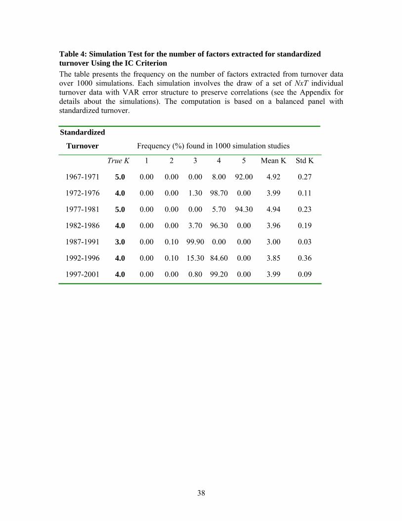
Table 4: Simulation Test for the number of factors extracted for standardized turnover Using the IC Criterion The table presents the frequency on the number of factors extracted from turnover data over 1000 simulations. Each simulation involves the draw of a set of NxT individual turnover data with VAR error structure to preserve correlations (see the Appendix for details about the simulations). The computation is based on a balanced panel with standardized turnover. Standardized

Turnover Frequency (%) found in 1000 simulation studies

True K 1 2 3 4 5 Mean K Std K

1967-1971 5.0 0.00 0.00 0.00 8.00 92.00 4.92 0.27

1972-1976 4.0 0.00 0.00 1.30 98.70 0.00 3.99 0.11

1977-1981 5.0 0.00 0.00 0.00 5.70 94.30 4.94 0.23

1982-1986 4.0 0.00 0.00 3.70 96.30 0.00 3.96 0.19

1987-1991 3.0 0.00 0.10 99.90 0.00 0.00 3.00 0.03

1992-1996 4.0 0.00 0.10 15.30 84.60 0.00 3.85 0.36

1997-2001 4.0 0.00 0.00 0.80 99.20 0.00 3.99 0.09

38

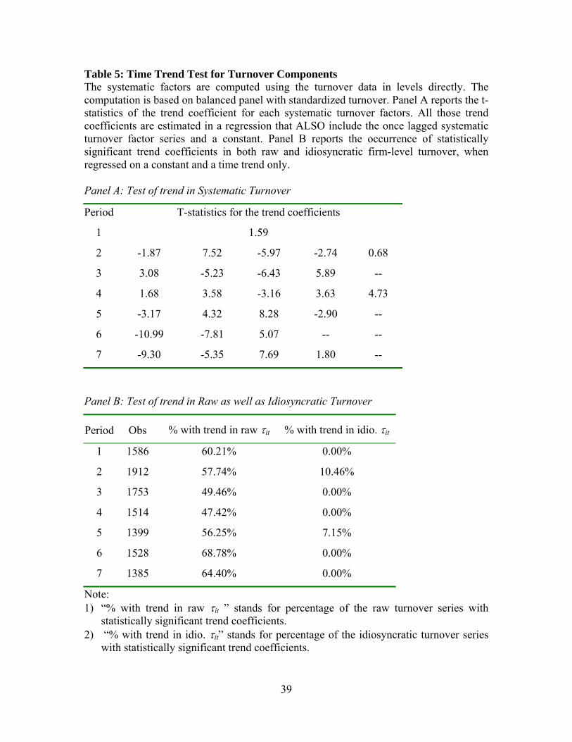
Table 5: Time Trend Test for Turnover Components The systematic factors are computed using the turnover data in levels directly. The computation is based on balanced panel with standardized turnover. Panel A reports the t-statistics of the trend coefficient for each systematic turnover factors. All those trend coefficients are estimated in a regression that ALSO include the once lagged systematic turnover factor series and a constant. Panel B reports the occurrence of statistically significant trend coefficients in both raw and idiosyncratic firm-level turnover, when regressed on a constant and a time trend only. Panel A: Test of trend in Systematic Turnover

Period T-statistics for the trend coefficients

1 1.59

2 -1.87 7.52 -5.97 -2.74 0.68

3 3.08 -5.23 -6.43 5.89 --

4 1.68 3.58 -3.16 3.63 4.73

5 -3.17 4.32 8.28 -2.90 --

6 -10.99 -7.81 5.07 -- --

7 -9.30 -5.35 7.69 1.80 --

Panel B: Test of trend in Raw as well as Idiosyncratic Turnover

Period Obs % with trend in raw τit % with trend in idio. τit

1 1586 60.21% 0.00%

2 1912 57.74% 10.46%

3 1753 49.46% 0.00%

4 1514 47.42% 0.00%

5 1399 56.25% 7.15%

6 1528 68.78% 0.00%

7 1385 64.40% 0.00%

Note: 1) “% with trend in raw τit ” stands for percentage of the raw turnover series with

statistically significant trend coefficients. 2) “% with trend in idio. τit” stands for percentage of the idiosyncratic turnover series

with statistically significant trend coefficients.

39

Table 6. Comparison Between Different Turnover Factors This table provides the average R2 from regressing individual stock turnover on separating turnovers from three asset pricing models: 1) CAPM, 2) Fama and French (1993), 3) a generic multi-factor model estimated from principal components (Lo and Wang, 2002). Performance in Panel A is computed as the average R2 of the model divided by the average R2 obtained from regressing individual stock turnover on principal components extracted from the turnover data. Performance in Panel B is computed as the average R2 of the model divided by the time-series average R2 obtained from regressing individual stock turnover on principal component betas estimated from the turnover data. The computation is based on balanced panel with standardized turnover. Panel A: Time Series Regression Of Individual Stock Turnover On Separating Turnovers CAPM Fama & French Lo and Wang

Time Average Stock R2

Performance Average Stock R2

Performance Average Stock R2

Performance

1 7.2% 28.4% 10.9% 42.7% 13.6% 53.5%

2 13.0% 48.6% 17.8% 66.4% 16.3% 60.8%

3 9.0% 39.1% 11.3% 48.9% 14.1% 60.8%

4 8.3% 39.7% 10.8% 51.5% 11.5% 54.9%

5 7.8% 42.5% 11.2% 60.9% 13.4% 73.0%

6 3.7% 24.2% 5.7% 36.5% 7.2% 46.6%

7 3.3% 16.4% 11.3% 55.4% 12.7% 62.4%

Panel B: Cross-Sectional Regression Of Individual Stock Turnover On Separating Turnover Betas

CAPM Fama & French Lo and Wang Principal

ComponentsTime Average R2 Performance Average R2 Performance Average R2 Performance Average R2

1 8.2% 39.6% 14.6% 70.8% 12.6% 60.8% 20.7%

2 5.5% 31.4% 13.7% 78.8% 11.2% 64.4% 17.4%

3 8.9% 50.0% 12.1% 67.9% 12.4% 69.5% 17.9%

4 6.1% 41.2% 11.0% 73.9% 9.5% 64.0% 14.9%

5 5.4% 42.1% 8.8% 69.0% 8.8% 68.9% 12.8%

6 7.6% 44.9% 10.0% 59.1% 12.9% 76.4% 16.9%

7 8.9% 47.6% 13.1% 69.9% 11.9% 63.6% 18.7%

40

Table 7: Simulation Results on the Test of Equal Number of Factors The table presents the Type I and Type II Error Estimates for test on the difference between the number of return factors and the number of turnover factors based on 1,000 simulations for each time period. Each simulation involves the draw of a set of NxT individual return and turnover data with VAR error structure to preserve correlations. The bold-faced numbers give the probability of error. The computation is based on a balanced panel with standardized turnover.

Panel A: Type I Error Estimates based on 1,000 Simulation for Each Time Period

Frequency (%) Found Time period

Specified

K-K’ -3 -2 -1 0 1 2

1 0 0.0 0.0 15.8 84.2 0 0.0

2 0 0.0 0.0 1.2 98.8 0 0.0

3 0 0.0 0.0 0.3 99.7 0 0.0

4 0 0.0 0.0 0 100 0 0.0

5 0 0.0 0.0 0 100 0 0.0

6 0 0.0 0.0 0 100 0 0.0

7 0 0.0 0.0 0.8 99.2 0 0.0

Panel B: Type II Error Estimates based on 1,000 Simulation for Each Time Period

Frequency (%) Found Time period

Specified

K-K’ -4 -3 -2 -1 0 1

1 -3 0 93.3 6.7 0 0 0

2 -2 0 1.5 97.2 1.3 0 0

3 -3 0.5 93.8 5.7 0 0 0

4 -2 0 0 96.3 3.7 0 0

5 -1 0 0 0 99.9 0.1 0

6 -2 0 0 84.6 15.3 0.1 0

7 -1 0 0 0.5 98.7 0.8 0

41

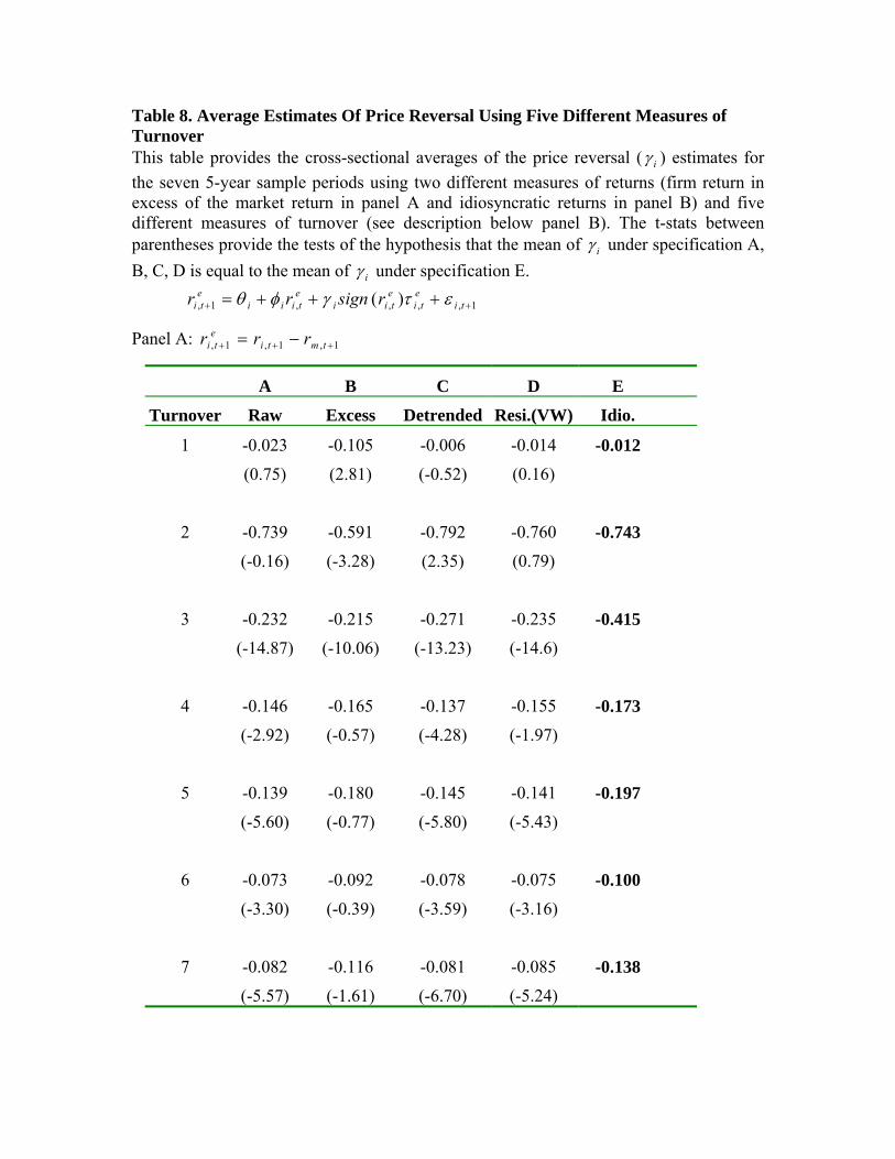
Table 8. Average Estimates Of Price Reversal Using Five Different Measures of Turnover This table provides the cross-sectional averages of the price reversal ( iγ ) estimates for the seven 5-year sample periods using two different measures of returns (firm return in excess of the market return in panel A and idiosyncratic returns in panel B) and five different measures of turnover (see description below panel B). The t-stats between parentheses provide the tests of the hypothesis that the mean of iγ under specification A, B, C, D is equal to the mean of iγ under specification E.

1,,,,1, )( ++ +++= tie

tietii

etiii

eti rsignrr ετγφθ

Panel A: 1,1,1, +++ −= tmtieti rrr

A B C D E

Turnover Raw Excess Detrended Resi.(VW) Idio.

1 -0.023 -0.105 -0.006 -0.014 -0.012

(0.75) (2.81) (-0.52) (0.16)

2 -0.739 -0.591 -0.792 -0.760 -0.743

(-0.16) (-3.28) (2.35) (0.79)

3 -0.232 -0.215 -0.271 -0.235 -0.415

(-14.87) (-10.06) (-13.23) (-14.6)

4 -0.146 -0.165 -0.137 -0.155 -0.173

(-2.92) (-0.57) (-4.28) (-1.97)

5 -0.139 -0.180 -0.145 -0.141 -0.197

(-5.60) (-0.77) (-5.80) (-5.43)

6 -0.073 -0.092 -0.078 -0.075 -0.100

(-3.30) (-0.39) (-3.59) (-3.16)

7 -0.082 -0.116 -0.081 -0.085 -0.138

(-5.57) (-1.61) (-6.70) (-5.24)

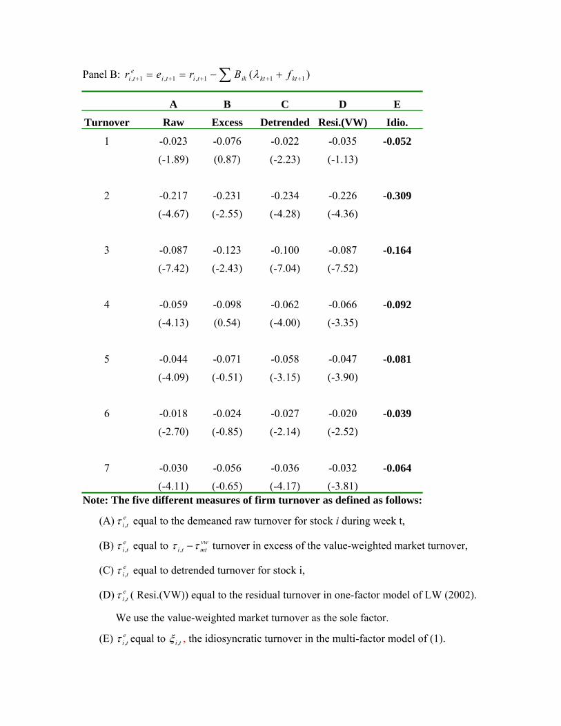
Panel B: ∑ +++++ +−== )( 111,1,1, ktktiktitieti fBrer λ

A B C D E

Turnover Raw Excess Detrended Resi.(VW) Idio.

1 -0.023 -0.076 -0.022 -0.035 -0.052

(-1.89) (0.87) (-2.23) (-1.13)

2 -0.217 -0.231 -0.234 -0.226 -0.309 (-4.67) (-2.55) (-4.28) (-4.36) 3 -0.087 -0.123 -0.100 -0.087 -0.164 (-7.42) (-2.43) (-7.04) (-7.52)

4 -0.059 -0.098 -0.062 -0.066 -0.092 (-4.13) (0.54) (-4.00) (-3.35) 5 -0.044 -0.071 -0.058 -0.047 -0.081 (-4.09) (-0.51) (-3.15) (-3.90)

6 -0.018 -0.024 -0.027 -0.020 -0.039 (-2.70) (-0.85) (-2.14) (-2.52)

7 -0.030 -0.056 -0.036 -0.032 -0.064 (-4.11) (-0.65) (-4.17) (-3.81)

Note: The five different measures of firm turnover as defined as follows:

(A) equal to the demeaned raw turnover for stock i during week t, eti,τ

(B) equal to turnover in excess of the value-weighted market turnover, eti,τ vw

mtti ττ −,

(C) equal to detrended turnover for stock i, eti,τ

(D) ( Resi.(VW)) equal to the residual turnover in one-factor model of LW (2002).

We use the value-weighted market turnover as the sole factor.

eti,τ

(E) equal to eti,τ ti,ξ , the idiosyncratic turnover in the multi-factor model of (1).

Figure 1a: Average Autocorrelations for EW Turnover Index (Raw and GRT detrended) and Individual Turnovers (Excess, Raw, Detrended, Residual (VW market model), and Idiosyncratic (multi-factor model)) The figure plots the cross-sectional averages of the first ten lags of the autocorrelation of seven different measures of firm-specific turnover (see their descriptions in the paper), for the 1997-2001 time period.

-0.10

0.00

0.10

0.20

0.30

0.40

0.50

0.60

0.70

0.80

0.90

1.00

ρ1 ρ2 ρ3 ρ4 ρ5 ρ6 ρ7 ρ8 ρ9 ρ10

Aut

ocor

rela

tion

EW Index-RawEW Index-GRTExcessRawResi(VW)DetrendIdiosyncratic

Figure 1b: Average Absolute Autocorrelations for Excess, Raw, Residual, Detrended, and Idiosyncratic Turnover The figure plots the cross-sectional averages of the first ten lags of the absolute autocorrelation of five different measures of firm-specific turnover (see their descriptions in the paper), for the 1997-2001 time period.

0

0.05

0.1

0.15

0.2

0.25

0.3

0.35

0.4

0.45

ρ1 ρ2 ρ3 ρ4 ρ5 ρ6 ρ7 ρ8 ρ9 ρ10

Aut

ocor

rela

tion Excess

RawResi(VW)DetrendIdiosyncratic