WSRC-SQP-A-00028

ii

TABLE OF CONTENTS

LIST OF TABLES....................................................................................................................................... iii

PURPOSE ..................................................................................................................................................... 1

SCOPE........................................................................................................................................................... 1

TERMS/DEFINITIONS .............................................................................................................................. 2

RESPONSIBILITIES .................................................................................................................................. 3

SOFTWARE LIFE CYCLE........................................................................................................................ 3

1.1 SOFTWARE REQUIREMENTS ............................................................................................................... 3 1.2 SOFTWARE DESIGN ............................................................................................................................ 4 1.3 SOFTWARE IMPLEMENTATION............................................................................................................ 4 1.4 SOFTWARE TEST ................................................................................................................................ 4 1.5 SOFTWARE INSTALLATION AND ACCEPTANCE ................................................................................... 5

1.5.1 Virus Checking ......................................................................................................................... 5 1.5.2 Checking PORFLOW into a Software Library......................................................................... 5 1.5.3 Installation of PORFLOW on the Analyst’s Computer Platform ............................................. 5 1.5.4 Acceptance Testing................................................................................................................... 6 1.5.5 Acceptance of PORFLOW........................................................................................................ 7 1.5.6 Documentation of Testing....................................................................................................... 14 1.5.7 User Instructions .................................................................................................................... 14

1.6 SOFTWARE OPERATION AND MAINTENANCE.................................................................................... 15 1.6.1 Operation................................................................................................................................ 15 1.6.2 Maintenance ........................................................................................................................... 15

1.7 SOFTWARE RETIREMENT.................................................................................................................. 15

CONFIGURATION CONTROL.............................................................................................................. 15

1.8 CONFIGURATION IDENTIFICATION.................................................................................................... 15 1.9 CONFIGURATION CHANGE CONTROL ............................................................................................... 16

1.9.1 Changes to PORFLOW .......................................................................................................... 16 1.9.2 Changes to/Creation of Test Data Sets................................................................................... 16 1.9.3 Changes in Hardware Configuration or Operating System ................................................... 16

1.10 CONFIGURATION CONTROL DOCUMENTATION ............................................................................ 17

QUALITY CONTROL FOR SOFTWARE MODELS........................................................................... 17

1.11 DEVELOPMENT AND REVIEW OF SOFTWARE MODELS.................................................................. 17 1.12 SIGN-OFF AND APPROVALS.......................................................................................................... 17 1.13 DOCUMENTATION TO DEMONSTRATE COMPLIANCE WITH QUALITY ASSURANCE PROCEDURES.. 17

PROBLEM REPORTING AND CORRECTIVE ACTION .................................................................. 18

RECORDS .................................................................................................................................................. 18

REFERENCES ........................................................................................................................................... 18

APPENDIX A. Virus Checking Results ................................................................................................... 19

APPENDIX B. Acceptance Testing Program .......................................................................................... 20

WSRC-SQP-A-00028

iii

APPENDIX C. Acceptance Testing Documentation .............................................................................. 23

APPENDIX D. Sample Batch File for Executing PORFLOW.............................................................. 33

LIST OF TABLES Table 1. Sign Convention for Flux Boundary Conditions............................................................. 25 Table 2. Sign Convention for Gradient Boundary Conditions ...................................................... 25

WSRC-SQP-A-00028

1

PURPOSE This plan describes the steps taken by SRTC, to implement software quality assurance (SQA) procedures, based on the ASME Nuclear Quality Assurance (NQA) standards, QA Manual 1Q, E7 5.xx and SRTC L1 8.20 requirements. This plan applies to the acquired computer code PORFLOW© version 4.00.7 (Runchal 1997). PORFLOW was classified as level D software in the Software Inventory Database and assigned the software identification L323-B-001V. SCOPE The SQA plan applies to life-cycle phases of PORFLOW as it is used for modeling various waste sites. Life-cycle phases include requirements, design, implementation, test, installation and acceptance, operation and maintenance, and retirement. Because this is pre-existing custom software purchased from a commercial vendor, the requirements, design and implementation phases are essentially descriptions of the program capabilities combined with sufficient testing to compensate for lack of design and implementation documentation. Configuration control is included in the SQA plan. This SQA plan does not cover auxiliary software, such as FACT, that produces results that become inputs to PORFLOW. This SQA plan is intended to cover the use of PORFLOW in all modeling applications. It is anticipated that those applications will include work for Solid Waste, such as waste disposal in any type of trench (including but not limited to direct disposal and disposal in cementitious settings, such as Components in Grout), Low-Activity Waste Vaults and the Intermediate Waste Vault, etc. This SQA Plan also explicitly covers any combination of these types of analyses such as the Composite Analysis. Other applications will include work for High-Level Waste concerning high-level waste tanks. PORFLOW may be used for other applications as well. This SQA plan is intended to be sufficiently robust to cover all those applications, but if the testing is not appropriate for a specific future application, then this SQA plan must be revised to include those applications or a specific SQA plan must be developed that is germane to that application. Because this SQA plan includes completed QA activities, plan reviewers and approvers must be technically qualified to have performed the work independently from the author. One special requirement is technical proficiency with Fortran90 to review the auxiliary program that was developed to compare the output of test cases.

WSRC-SQP-A-00028

2

TERMS/DEFINITIONS ANALYST The Analyst is the person having overall technical responsibility for computer simulations used for modeling, e.g., waste site flow and contaminant transport simulations. The analyst and the Principal Investigator can be the same person. CONFIGURATION CONTROL Configuration control is the process of identifying and defining the configuration items in a system, controlling the release and change of these items throughout the system's life cycle, and recording and reporting the status of configuration items and change requests. PORFLOW PORFLOW is a commercially available computer code acquired by WSRC for use in simulating ground water flow and contaminant transport in the vadose zone and underlying aquifers. Examples of simulation results are contaminant concentrations and ground water and contaminant fluxes to seeplines at Upper Three Runs Creek and Four Mile Branch for contaminants originating from low-level or high-level waste sites. PRINCIPAL INVESTIGATOR (PI) The principal investigator is the individual responsible for coordinating tasks to be completed by SRTC for modeling activities. The PI and the analyst can be the same person. The PI performs all roles of the Cognizant Technical Function identified in procedures. SOFTWARE Software refers to computer programs, including source and executable codes, procedures, rules, and associated documentation and data pertaining to the operation of a computer system. Software includes the media for storing the software. The data for PORFLOW includes constants and other information encoded with the program instructions. The license file and the initialization file are the only external sources of data that are an integral part of the program itself. Software is separate from hardware consisting of computers and related equipment. SOFTWARE BENCHMARKING Benchmarking is testing results for complex computer models against results from similar computer programs that are accepted and used in the ground water modeling industry. SOFTWARE MODEL A software model is the specific problem input to the software program. A software model is defined here as the numerical model consisting of a mesh with associated material properties, boundary conditions, and initial conditions. The software model describes the problem to be solved in a manner that the software code can interpret. The software code consists of the program of instructions that is used to generate simulation results based on

WSRC-SQP-A-00028

3

the software model that feeds it. SOFTWARE VALIDATION Validation is the test and evaluation of the completed software to ensure compliance with software requirements. This consists of testing the accuracy of numerical algorithms coded in the software using simple models. QA Manual 1Q also states that “software verification shall be performed throughout the life cycle to ensure that the products of a given life cycle phase fulfill the requirements of the previous phase or phases.” This requirement does not apply because PORFLOW is delivered as a completed product. SOFTWARE FIELD VALIDATION Field validation is testing the accuracy of results predicted by computer models with field conditions and results. RESPONSIBILITIES ANALYST The analyst is responsible for providing technical expertise to the PI. The analyst is responsible for determining software compatibility with existing or acquired hardware and for defining software needs, e.g., memory requirements. The analyst is responsible for installing and testing software. PRINCIPAL INVESTIGATOR The PI is responsible for identifying the need for creating and revising SQA plans and procedures. The PI is responsible for classifying software and establishing software custodial requirements. The PI is responsible for overseeing that the software life-cycle procedures are correctly implemented, including configuration control and quality control. The PI is responsible for determining that this SQA plan is appropriate for the intended type of application. If that type of application is explicitly mentioned in this SQA plan then this SQA plan is applicable. If that type of application is not explicitly mentioned in this SQA plan, then the PI must document the reasons why this SQA plan is applicable to the intended type of application. Documentation may be included as part of a revised SQA plan, an analysis report or as a stand-alone item. SOFTWARE LIFE CYCLE

1.1 Software Requirements Because Porflow is commercially available software, the software requirements consist of a description of the capabilities needed to analyze the conditions at the Savannah River Site.

WSRC-SQP-A-00028

4

The salient features of Porflow are described to ensure that they provide sufficient capabilities. This section also provides the acceptance criteria. The primary functional requirements of the software are that it must be capable of simulating groundwater flow and contaminant transport through the subsurface in both the vadose zone and the aquifer system. The software must be able to simulate generation of progeny for radionuclides. Transient and steady state scenarios must be accommodated. Reporting capabilities for concentrations, fluxes and mass balances are needed The following quote from Porflow Capabilities, Usage History, And Testing (Collard, 1998) shows some of the salient features of Porflow that indicate that PORFLOW provides sufficient capabilities to satisfy the software requirements: “The PORFLOW computer program is numerical analysis software that can model ground water flow and contaminant and heat transport through the environment. PORFLOW readily accommodates multiple chemical species, radioactive decay chains, transient and steady-state flow conditions, saturated and unsaturated media, multiple material types, and one, two or three dimensional geometries of any shape.” The acceptance criteria in general are that test examples execute properly and demonstrate that PORFLOW can adequately solve relatively simple problems that address the primary functional requirements stated above. Extensive PORFLOW testing has been accomplished previously. Collard (1998) reported on the testing and formal reviews that have been accomplished for PORFLOW. ACRI (1994) published a validation report for an earlier version of PORFLOW. The test cases in that validation report form the basis for the acceptance criteria. They are discussed in further detail in the Installation and Acceptance section.

1.2 Software Design Because PORFLOW is purchased software the design is not considered here. The test and acceptance stage must compensate for the lack of access to design information.

1.3 Software Implementation Because PORFLOW is purchased software the implementation is not considered here. The implementation phase develops the software products, which for PORFLOW already exist.

1.4 Software Test This phase of the life cycle is required to ensure that the software was developed correctly.

WSRC-SQP-A-00028

5

This phase is required before porting the software to its final destination that may be a similar computer platform, a dissimilar computer platform or computerized equipment. This test is can only be performed on the original computer where the software was developed. This test is not applicable to purchased software, but equivalent testing must be accomplished during Software Installation and Acceptance on the computer platform used to perform analyses.

1.5 Software Installation and Acceptance The Porflow software was checked for viruses, placed in a software library, and was installed on the Analyst’s computer. After installation, test cases were executed to ensure that Porflow worked properly.

1.5.1 Virus Checking Because PORFLOW is pre-existing software, tests must be conducted to assure the software is free of viruses that may infect the computer system on which it is installed. PORFLOW was found to be free of viruses as documented in Appendix A.

1.5.2 Checking PORFLOW into a Software Library The software was saved in the SafeSource database operated by P&CT. SafeSource acts as a library so that the analyst can check out a copy of the software. A report on the security for the server running SafeSource and the protections of backup media including, but not limited to theft, loss, and environmental damage is in preparation (Van Alstine, 2002).

1.5.3 Installation of PORFLOW on the Analyst’s Computer Platform Installation was accomplished by following the vendor’s recommendations. Installation consisted merely of copying the software to a directory on the computer. Three files were included in the software package as described below: Acrinit.acr - an initialization file adapted to each user PORFLOW.EXE - the executable program WHS_LCNS - the license file The user makes no changes to any of these files. Generally the initialization file and the license file would reside in the current working directory where an input model is analyzed. Simple batch files can copy these two files to the working directory and then delete the files from the current working directory after the analysis is completed.

WSRC-SQP-A-00028

6

1.5.4 Acceptance Testing Testing is required to confirm that PORFLOW satisfies the objectives and requirements of the simulations to be conducted. QA Manual 1Q states that testing shall include “test cases encompassing the range of permitted usage defined by the program documentation.” The extent of the testing for PORFLOW will be more limited, because some capabilities of PORFLOW may never be used at SRS and testing those capabilities would provide no benefit. If the PI intends to use PORFLOW capabilities that have not previously been tested, then those capabilities generally must be tested before PORFLOW is applied in that application (unless for example, that application is a scoping study). If PORFLOW is used for an application that is explicitly listed in the Appendix C conclusions, then specific documentation on its suitability is not required, otherwise, the suitability for use must be documented by the PI. QA Manual 1Q also discusses negative impacts from the software. Because PORFLOW does not control any equipment, it has been checked for viruses, and it only affects the computer on which it is executed, the worst that can happen to the system is to crash the computer. This event does not permanently degrade the system because a system restart will restore the system, thus the possible negative impacts are insignificant. Even though PORFLOW produces correct results for the test cases (discussed later in this section) and thus satisfies QA Manual 1Q, incorrect or atypical results can occur during actual application of the software. In other words, it is impossible for the test cases to anticipate all operating scenarios and conditions. During previous applications, PORLFOW produced mathematical overflow errors on occasion and output very small numbers in scientific notation that do not include the “E” for the exponent, e.g., 1.2-111. The mathematical overflow stops processing, thus this abnormal condition is adequately handled by the software, because the analyst cannot be mislead by incorrect output results. The very small numbers produce errors for many post-processing programs that read the numbers with prescribed format statements. However, those numbers can be read using list-directed input in Fortran, thus a method exists for dealing with this abnormal condition. QA Manual 1Q discusses various methods for evaluating the adequacy of the software test case results. The primary method used to evaluate PORFLOW results is to compare them to “standard problems with known solutions.” The PORFLOW validation manual provides detailed discussions of test cases and how they were compared to closed-form solutions, to experiments, or to results from other well-recognized computer programs. Because in-depth comparisons were already completed and documented in the PORFLOW validation manual, sufficient acceptance testing only requires comparing output from the software installed on the final platform to output from previous validation testing. ACRI,

WSRC-SQP-A-00028

7

the author of PORFLOW, provides both input and output files for the test cases. A small program, QaPor, was written to automate output file comparisons between the vendor’s output files and output files generated by the installed software. The source code for that program is included as an Appendix B. QaPor does a character-by-character comparison, but it ignores specific data that naturally change each time the program is executed. The ignored data are as follow:

DATE DATE OF RUN License Number Licensed To Registered User Licensed Use ELAPSED TIME FOR THIS CASE CPU TIME FOR THIS CASE CPU TIME IN LINEAR SOLVER TIME PER GRID NODE PER STEP TIME PER NODE-STEP-EQUATION

1.5.5 Acceptance of PORFLOW Section 1.2 of the PORFLOW validation manual, ACRI (1994) contains verification test problems and benchmark test problems. Descriptions of these test problems extracted from the validation manual are provided below for convenience.

1.2 OVERVIEW OF TEST PROBLEMS 1.2.1 Verification Test Problems Problem V1: Transient One-Dimensional Diffusion: This problem simulates the diffusive transport of a contaminant in a homogeneous, semi-infinite slab. The contaminant concentration at the right edge of the slab is maintained at a constant value. The left edge is insulated so that no contaminant enters or leaves the boundary. An analytic solution for this problem is given by Carslaw and Jaeger (1959). This problem tests the diffusive transport component of the PORFLOW algorithm.

WSRC-SQP-A-00028

8

Problem V2: Heat Transfer in Unidirectional Flow: In this test, advective, diffusive and dispersive heat transfer in a saturated porous medium is simulated. The computational domain consists of a horizontal slab with unidirectional flow from left to right. Initially, the temperature is uniform throughout the domain. At time t=0, water with a higher temperature begins entering the computational domain from the left boundary. The analytic solution for this problem is given by Carslaw and Jaeger (1959). The problem, as formulated, is attributed to Avdonin (1964) and has been used previously for verification of computer codes by several authors. The primary objective of this problem is to test the ablility of PORFLOW to correctly simulate coupled advective and dispersive transport. Problem V3: Theis Solution for Transient Drawdown: This classic problem (Theis, 1935) simulates the transient drawdown of pressure head due to pumping in a homogeneous, confined aquifer of constant thickness that is fully penetrated by a well. The problem was originally posed and solved by Theis with the assumption that the flow is radial. It tests the ability of PORFLOW to correctly propagate a pressure transient in a radial geometry. Problem V4: Finite Cylinder with Heat Source: This problem involves a finite cylinder in which heat is generated at a constant rate while the surface of the cylinder is maintained at zero temperature. The purpose of this test is to determine the ability of PORFLOW to simulate heat sources. The analytic solution for this problem is described by Carslaw and Jaeger (1959). Problem V5: Convective Heat Transfer in Regional Flow: This problem concerns a homogenous, isotropic, vertical cross-section of a region with a geothermal gradient. The geothermal heat flux enters the region from the bottom and leaves through a constant temperature surface at the top. The region is bounded on its two vertical faces with topological divides such that there is no major lateral flow. A recirculating flow pattern is induced due to lateral variations in the water table. This problem was formulated and solved by Domenico and Palciauskas (1973). The objective of the problem is to test the capability of the PORFLOW algorithm to predict convective heat transfer in the presence of a non-uniform flow field. Problem V6: Three-Dimensional Contaminant Transport: This problem simulates the transport of a contaminant in a three-dimensional domain. A finite source near the upper surface of the computational domain continuously releases a contaminant into an aquifer that initially is free of the contaminant. The flow within the aquifer is unidirectional. Advective transport moves the contaminant in the downstream direction, while dispersive movement causes spreading of the contaminant in all directions. An analytic solution for this problem was obtained by Codell et al. (1982). This problem tests the ability of PORFLOW to simulate three dimensional advective and dispersive transport of a contaminant from a finite source. Problem V7: Philip's Horizontal Unsaturated Flow: The physical setting for this problem is a horizontal slab of homogeneous, isotropic soil. The vertical extent of the slab is infinite. Initially, the soil is partially saturated with ground water. At time t=0, the saturation at the left boundary is increased to unity. This saturation front then migrates downstream. The objective of this problem is to test the ability of PORFLOW to correctly compute a propagating saturation front in the absence of gravitational effects. An analogous problem was first formulated and analytically solved by Philip (1957a). Problem V8: Philip's Vertical Unsaturated Column: The physical setting for this problem is a vertical column of homogeneous, isotropic soil. The horizontal extent of the column is considered to be infinite. The soil is initially partially saturated. At time t=0, the saturation at the top boundary is increased to unity. Transient infiltration of moisture in the vertical direction results

WSRC-SQP-A-00028

9

from capillary forces and gravity. An analytic solution for an analogous problem with a propagating front was obtained by Philip (1957b). This problem tests the ability of PORFLOW to correctly simulate a migrating saturation front in the presence of gravitational effects. Problem V9: Infiltration from a Line Source: This problem describes the flow from a single subsurface irrigation pipe that is located in an unsaturated zone above a shallow water table. Due to the infinite extent of the problem along the direction of the porous pipe, this three-dimensional problem with a line source is mathematically equivalent to a two-dimensional problem with a point source. An approximate analytic solution for this problem is given by Warrick and Lomen (1977). The objective of this problem is to evaluate the ability of PORFLOW to correctly simulate flow and saturation distribution in a variably-saturated, two-dimensional domain. Problem V10: Free-Surface Boussinesq Flow with Recharge: This problem concerns a semi-infinite, unconfined aquifer. Initially, the phreatic surface is horizontal everywhere. At time t=0, the water level at the left boundary is suddenly raised. A compression wave, consisting of an elevated phreatic surface, then propagates from left to right in a transient manner. This problem is often referred to as the Boussinesq problem. It is described in detail by Polubarinova-Kochina (1954). The objective of this test is to determine the ability of PORFLOW to correctly model a compression wave in an unconfined aquifer. Problem V11: Free-Surface Boussinesq Flow with Seepage: This test problem is a variation of the previous Boussinesq problem. In this test case also, the initial phreatic surface is horizontal everywhere. At time t=0, the water level at the left boundary is suddenly lowered. An expansion wave, consisting of a lowered phreatic surface, then propagates from right to left in a transient manner. The objective of this test is to determine the ability of PORFLOW to correctly simulate an expansion wave in an unconfined aquifer.

1.2.2 Benchmark Test Problems Problem B1: Two-Dimensional Transient Infiltration: This problem considers flow through a two dimensional, rectangular column of partially saturated soil. The right vertical face of the column is held at its initial pressure head, while the pressure in the upper part of the left vertical face is increased. The lower part of the left face is impermeable. This causes a two-dimensional saturation front to propagate from left to right. This problem was proposed by Ross et al. (1982) for benchmark testing of computer codes. Pruess (1987) has solved this problem numerically with the TOUGH computer code. It tests the ability of PORFLOW to correctly simulate saturation fronts propagating in two dimensions. Problem B2: Two-Dimensional Steady-State Infiltration: This problem concerns the steadystate movement of moisture under variably saturated flow conditions. The physical setting for the problem is a vertical cross-section of an aquifer with a regional hydrologic gradient. The lateral extent of the aquifer is assumed to be infinite and only a unit width is considered. Recharge occurs at the left boundary and the flow discharges at the right boundary. Additional recharge occurs through infiltration at the surface. The problem is described by Magnuson et al. (1990) and has been used as a benchmark problem for several codes. The FEMWATER computer code by Yeh and Ward (1979) was used as a benchmark for comparing the PORFLOW results. This problem tests the ability of PORFLOW to compute two-dimensional, variably saturated flow with infiltration.

Problem B3: Jornada Test Trench Simulation: This problem is based on the field tests conducted at the Jornada Test Site near Las Cruces, New Mexico. The test involves transient, two-

WSRC-SQP-A-00028

10

dimensional infiltration of water into an extremely dry heterogeneous soil. The physical setting and hydraulic properties of the soil are described by Smyth et al. (1989). The test area comprises three layers of soil which vary in material and hydrologic properties. Additionally, a small zone of high conductivity soil is contained within the lowermost soil layer. The experiment was conducted under the direction of Dr. Peter Wierenga of the University of Arizona. Smyth et al. (1989) numerically solved four problems of increasing complexity using the TRACER3D computer code. The problem considered here is the fourth and most complex of these problems. It was also numerically solved by Magnuson et al. (1990) using the TRACER3D, FLASH and PORFLOW (Version 1.00) computer codes. This problem tests the ability of PORFLOW to correctly simulate variably saturated flow with infiltration in inhomogeneous soil under extremely dry conditions.

Problem B4: Saltwater Intrusion into a Confined Aquifer: This problem deals with the intrusion of seawater into a confined fresh water aquifer. The problem was described by Henry (1964) who obtained a Fourier-Galerkin solution from an idealized mathematical model. Fresh water recharge occurs at a constant rate at the left boundary of an aquifer. The right boundary is a seawater interface with hydrostatic pressure. No fluid enters or leaves through the top and bottom boundaries. The fluid density varies as a linear function of salinity. A Ghyben-Herzberg lens is formed due to the interaction of the buoyancy forces, freshwater recharge and salinity dispersion. This problem has been used extensively for verification of computer models (Pinder and Cooper, 1970; Segol et al, 1975; Huyakorn and Taylor, 1976; Desai and Contractor, 1977; INTERA, 1979; Frind, 1982, Voss, 1984; Sanford and Konikow, 1985). This problem tests the ability of PORFLOW to simulate strongly coupled, density-driven, flow and solute transport.

Problem B5: Saturated Flow in a Fractured Porous Medium: This problem concerns steadystate flow in a saturated, geologic medium with discrete embedded fractures. The hydraulic properties of the medium are based on core test data on basalts from the Idaho National Engineering Laboratory. The physical setting and the boundary conditions are selected to assure hydraulic interaction between the discrete fractures and porous medium. The computational domain contains two vertically oriented discrete fractures. The fractures are separated from each other and from the boundaries of the computational domain. The hydraulic conductivity of each fracture is more than 5 orders of magnitude larger than that of the porous media. This problem was originally devised and numerically solved by Magnuson et al. (1990) using the FLASH and PORFLOW (Version 1.00) computer codes. It tests the ability of PORFLOW to simulate flow in a porous media with embedded fractures of very high hydraulic conductivity.

Problem B6: Flow to a Geothermal Well: The physical setting for this problem is a geothermal well with production at a constant rate. Initially the reservoir is in single phase conditions. As the well is produced, pressure drops to the saturated vapor pressure creating two phase liquid-vapor conditions. This leads to a boiling front which propagates outward from the well into the reservoir. Garg (1978) developed a semi-analytic theory for radial flow to a geothermal well. A modified version of Garg's Problem was used at the Stanford Geothermal Program (1980) for a comparative study of reservoir simulators. Pruess (1987) obtained a numerical solution for this problem with the TOUGH computer code. It tests the ability of PORFLOW to simulate porous media flow with evaporation, and the propagation of a boiling front.

Input data for these and other problems are provided in PORDEMO.DAT. Titles of all test cases in PORDEMO.DAT are as follows:

CHAPTER 1: SATURATED FLOW PROBLEMS

WSRC-SQP-A-00028

11

TITLe CASE 1.01 - Transient Pressure Decay to Zero TITLe CASE 1.02 - Uniform Velocity with Pressure + Normal Grad B.C. TITLe CASE 1.03 - Linear U + Linear T with Heat Source TITLe CASE 1.04 - Rectangular Rod with Fixed End Temperatures TITLe CASE 1.05 - Cylindrical Ring with Fixed End T and C TITLe CASE 1.06 - End Temperature Fixed Uniform Velocity Field TITLe CASE 1.07 - Comparison of ADI Results with SOR (Next Set) TITLe CASE 1.08 - Comparison of SOR Results with ADI (Previous Set) TITLe CASE 1.09 - Bouyancy Affected Flow in a HLW Repository CHAPTER 2: UNCONFINED FREE SURFACE FLOW PROBLEMS TITLe CASE 2.01 - Boussinesq Transient-State Problem: Areal Mode CHAPTER 3: FRACTURE FLOW PROBLEMS TITLe CASE 3.01 - Skin Tests for Dr. Heidung TITLe CASE 3.02 - Skin Tests for Dr. Heidung TITLe CASE 3.03 - Skin Tests for Dr. Heidung TITLe CASE 3.04 - Skin Tests for Dr. Heidung CHAPTER 4: VARIABLY SATURATED FLOW PROBLEMS TITLe CASE 4.01 - Vertical Infilteration with Rainfall TITLe CASE 4.02 - Philip's Infiltration Problem TITLe CASE 4.03 - T-106 Single-Shell Tank Benchmark Problem CHAPTER 5: VARIABLY SATURATED MULTI-PHASE PROBLEMS TITLe CASE 5.01 - Three Phase Flow: Transmission Oil-Water-Air Simulation of PNL Experimental Data CHAPTER 6: PROBLEMS WITH FREEZING AND THAWING TITLe CASE 6.01 - Neumann's Freezing Test Case Analytic solution by Jumikis TITLe CASE 6.02 - Stefan Problem Analytic solution given by: Lunardini, V.J. (1981). Heat Transfer in Cold Climates TITLe CASE 6.03 - Buried Warm Pipe in Homogeneous Soil without Insulation CHAPTER 7: PROBLEMS WITH NON-ORTHOGONAL GRIDS TITLE CASE 7.01: PARALLELOPIPED CAVITY WITH MOVING WALL - March 2, 1996 TITLE CASE 7.02: FLOW AND HEAT TRANSFER IN AN ANNULAR SPACE TITLE CASE 7.04: FLOW IN A TRAPIZOIDAL SPACE CHAPTER V: VERIFICATION PROBLEMS IN THE PORFLOW MANUAL TITLe CASE V.01 – Transient One-Dimensional Diffusion

WSRC-SQP-A-00028

12

Carslaw, H.S. and J.C. Jaeger, 1959. Conduction of Heat in Solids TITLe CASE V.02 – One-Dimensional Heat Transport by Unidirectional Flow Carslaw, H.S. and J.C. Jaeger, 1959. Conduction of Heat in Solids Oxford Press 2nd Ed., pp. 387-389 TITLe CASE V.03 – Theis Solution for Transient Drawdown Theis, C.V., 1935. The Relation Between the Lowering of the Piezometric Surface and the Rate and Duration of Discharge of a Well Using Groundwater Storage, Trans. Amer. Geophys. Union, 2, p. 519-524. TITLe CASE V.04 – Finite Cylinder with Heat Source Carslaw, H.S. and J.C. Jaeger, 1959. Conduction of Heat in Solids Oxford Press 2nd Ed., p. 223-224 TITLe CASE V.05 – Coupled Flow and Heat Transfer in Regional Flow Domenico, P.A. and V.V. Palciauskas, 1973. Theoretical Analysis of Forced Convective Heat Transfer in Regional Ground-Water Flow, Geological Society of America Bulletin, Vol. 84, p. 3803-3814, December 1973. TITLe CASE V.06 – Three-Dimensional Transport of a Contaminant Codell, R.B., T.K. Key and G. Whelan, 1982. A Collection of Mathematical Models for Dispersion in Surface Water and Groundwater, NUREG-0868, Division of Engineering, Office of Nuclear Reactor Regulation, Washington, D.C. TITLe CASE V.07 – Philip's Solution for Horizontal Unsaturated Flow Philip, J.R., 1957. Numerical Solution of Equations of the Diffusion Type with Diffusivity Concentration-Dependent, Transactions, Faraday Society 51:885-892. TITLe CASE V.08 – Philip's Solution for a Vertical Unsaturated Column Philip, J.R., 1957. Numerical Solution of Equations of the Diffusion Type with Diffusivity Concentration-Dependent II, Australian Journal of Physics, 10(2), p 29-42. TITLe CASE V.09 – Infiltration from a Line Source to a Water Table Warrick, A.W. and D.O. Lomen, 1977. Flow from a Line Source above a Shallow Water Table, Soil Sci. Soc. Am. J., 41, p. 849-852. TITLe CASE V.10 – Transient Free-Surface Boussinesq Flow – Recharge Polubarinova-Kochina, P.Ya., 1954. Theory of Groundwater Movement, Translated from Russian to English by J.M. Roger de Weist, 1962, Princeton University Press, N.J. TITLe CASE V.11 – Transient Free-Surface Boussinesq Flow – Seepage Polubarinova-Kochina, P.Ya., 1954. Theory of Groundwater Movement, Translated from Russian to English by J.M. Roger de Weist, 1962, Princeton University Press, N.J. CHAPTER B: BENCHMARK PROBLEMS IN THE PORFLOW MANUAL TITLe CASE B.01 – Two-Dimensional Transient Infiltration Ross, B., J.W. Mercer, S.D. Thomas, and B.H. Lester, 1982. Benchmark Problems for Repository Siting Models, NRC-report NUREG/CR-3097, December, 1982. TITLe CASE B.02 - Two-Dimensional Steady-State Infiltration Magnuson S.W., R.G. Baca & A.J. Sondrup, August 1990. Independent Verification and Benchmark Testing of The PORFLO-3 Computer Code,

WSRC-SQP-A-00028

13

Version 1.0, EGG-BG-9175; INEL, Idaho Falls, ID 83415. TITLe CASE B.03 - Jornada Test Trench Simulation Magnuson S.W., R.G. Baca & A.J. Sondrup, August 1990. Independent Verification and Benchmark Testing of The PORFLO-3 Computer Code, Version 1.0, EGG-BG-9175; INEL, Idaho Falls, ID 83415. TITLe CASE B.04 - Saltwater Intrusion into a Confined Aquifer Henry, H.R., 1964. Effects of Dispersion on Salt Encroachment in Coastal Aquifers, Sea Water in Coastal Aquifers, U.S. Geological Survey Water Supply Paper 1613-C, p. C71-C84. TITLe CASE B.05 - Saturated Flow in a Fractured Porous Medium Magnuson S.W., R.G. Baca & A.J. Sondrup, August 1990. Independent Verification and Benchmark Testing of The PORFLO-3 Computer Code, Version 1.0, EGG-BG-9175; INEL, Idaho Falls, ID 83415. TITLe CASE B.06A - Flow to a Geothermal Well Pruess, K., 1987. TOUGH Users Guide. NUREG/CR-4645. U.S. Nuclear Regulatory Commission (NRC), Washington, D.C. (Problem 4) TITLe CASE B.06B - Flow to a Geothermal Well Pruess, K., 1987. TOUGH Users Guide. NUREG/CR-4645. U.S. Nuclear Regulatory Commission (NRC), Washington, D.C. (Problem 4)

The chapters with verification and benchmark problems are of primary interest here, because they have been documented (ACRI, 1994). ACRI provides additional test cases in PORT.DAT for newer PORFLOW versions. These test cases were not validated for PORFLOW version 4.00.7. PORT.DAT contains 20 undocumented test cases that demonstrate specific features of PORFLOW. The titles for the 20 test cases are as follow: 1. Solubility Limited Source 2. Solubility Limited Source 3. Solubility Limited Source 4. Decay 5. Precipitation from Liquid to Solid 6. Uptake from Solid to Liquid 7. Uptake from Solid to Liquid 8. Precipitation from Liquid to Solid 9. Precipitation from Liquid to Solid 10. Precipitation from Liquid to Solid 11. 2D Precipitation with Flow 12. 2D Precipitation with Flow 13. Precipitation with the Solid Concentration a Function of a Variable 14. History Options 15. History Options – Initial Read from Steady 16. Radiation Source Type 17. History Storage and History Source 18. Contaminant Transport Demonstration 19. Contaminant Transport Demonstration 20. Precipitation with Transport and Filiation

WSRC-SQP-A-00028

14

1.5.5.1 Validation Validation testing demonstrates whether the completed PORFLOW meets the requirements specified regarding function, performance, external interfaces and attributes. PORFLOW capabilities generally are validated by comparing output of the desired simulation equations for a defined problem to a published analytical solution. The comparison evaluates the accuracy of numerical algorithms for simple problems. In lieu of directly comparing output with published analytical solutions, output may be compared with output from versions of the same program that were previously validated, or compared with output from similar programs that were previously validated. For more complex problems that do not have an analytical solution, PORFLOW results are benchmarked against results from software that has gained high acceptability in the groundwater modeling arena.

1.5.5.2 Field Validation Field validation of PORFLOW requires data that not only test the ability of the codes to predict contaminant transport under present conditions, but also test the predictability of results when perturbations are made to the vadose zone and ground water system. Typically, these data are not readily available, especially when computer models are used to predict conditions thousands of years into the future. However, field data, where available, can be compared with model predictions. Such data are available from vadose zone monitoring instruments. That data can be used to revise or calibrate the model to improve predictions. If long-term predictions are based on average data (e.g. rainfall) and extreme conditions are encountered (e.g. drought or flooding) that data may require that a separate model be developed and calibrated. Information from the calibration of the second model could then be used to adjust, but not fully calibrate the first model.

1.5.6 Documentation of Testing Results of validation tests of PORFLOW shall be published as part of the SQA plan, part of an analysis report, or as a standalone document. The PI will maintain all documentation that is not available through Records Administration, Engineering Document Control, or the Software Administrator. Testing documentation is provided in Appendix C.

1.5.7 User Instructions User instructions can be found in the PORFLOW user’s manual (Runchal, 1997). A general batch file to copy the license and initialization file, execute PORFLOW, and delete the copied files is provided in Appendix D.

WSRC-SQP-A-00028

15

1.6 Software Operation and Maintenance

1.6.1 Operation The PI approves the analysts who will operate PORFLOW. These analysts will have access to the software, the user’s manual and all other documentation. Operational tests will be performed whenever PORFLOW is installed on a different computer and results will be used for final project reports that are not part of a scoping study, or when configurational changes are made to the software or hardware system. The results of these tests will be documented in a manner similar to that for validation testing.

1.6.2 Maintenance Maintenance to correct software errors or to adapt to changes in software requirements or the operating environments will be made only with the PI's approval, and will be documented. Written requests for maintenance actions will be kept in a location specified by the PI. PORFLOW changes can only be made by the vendor, because SRS does not have access to the source code.

1.7 Software Retirement Software will be placed in a standby state when new versions are obtained. Older versions will be archived and retained for a sufficient length of time to satisfy customer requirements for individual projects. When software is no longer required, it will be retired by returning it to the licenser or disposing it in accordance with instructions from the licenser and existing SRTC procedures. CONFIGURATION CONTROL Configuration control shall be initiated. The name of the software and the PI are recorded in the Software Inventory Database. The date of installation, version installed, and installation notes are recorded by the PI. Source code listings (if available), software documentation and user's manuals will be stored in a location accessible to designated users of the software, and shall not be removed without permission of the PI.

1.8 Configuration Identification A configuration baseline shall be defined for PORFLOW. Test cases shall be described by test input data sets, simulation results, and the hardware and operating system. The

WSRC-SQP-A-00028

16

hardware and operating system and the PORFLOW executable code used in the testing will define the configuration baseline. A labeling system will be implemented for each of these types of data files, such that each file is uniquely identified and such that configurations resulting from revisions of each file are uniquely identified.

1.9 Configuration Change Control Changes to configuration items, including the PORFLOW codes, test input data sets, operating systems and hardware shall be formally documented under the guidelines provided below.

1.9.1 Changes to PORFLOW The PI must approve changes to the baseline version of PORFLOW. Acceptance testing (as described in Section 1.5.4) shall be performed to ensure that testing results remain accurate for code changes.

1.9.2 Changes to/Creation of Test Data Sets Changes to, or creation of, new test data sets will be documented in a manner that uniquely identifies each set and corresponding simulation results.

1.9.3 Changes in Hardware Configuration or Operating System Changes to hardware or the operating system may affect the operation of PORFLOW. Therefore, such changes shall be accompanied by testing the current PORFLOW version with the new hardware or operating system. If no significant changes in results are found, then the configuration changes will be documented, with no further action being required. If significant changes in results are found, then the software will be recompiled, if possible, to create a new version and it will be retested. If no changes for the new version are found, then the configuration changes will be documented and the new software version will be archived. If changes are found, they will be investigated and addressed. If needed, the software author will be contacted to help resolve any remaining discrepancies. Changes to portions of the operating system that are not expected to affect software results need not be tested. An example is an update of registry information from installing new software utilities. On the other hand, installation of a new version of an operating system, e.g., a new version of Windows, will require a new round of testing.

WSRC-SQP-A-00028

17

1.10 Configuration Control Documentation Configuration control documentation shall contain the information needed to manage the PORFLOW configurations and accompanying data sets, simulation results and hardware requirements. This information shall identify the approved configuration (via a well documented naming convention for software, data sets, and simulation results) and will be kept in an SQA Logbook. The Logbook must clearly list and describe modifications made to the various configurations. QUALITY CONTROL FOR SOFTWARE MODELS

1.11 Development and Review of Software Models The Analyst shall develop and document the approach and key assumptions, and evaluate input data sets to assure that QA procedures have been applied and that proper documentation is being generated during the operational phase of the PORFLOW life cycle. When necessary, the Analyst will have other qualified analysts review assumptions and input data to verify their appropriateness and accuracy.

1.12 Sign-off and Approvals Sign-off and approvals for review of software models shall be determined on a project-by-project basis. The review process may range from being highly formal to very informal, depending on the importance of the project. For a formal process, it is suggested that sign-off and approvals on key assumptions and input data can be accomplished with correspondence transmitting the information being approved. The Analyst would identify reviewers. They would include managers and individuals with modeling experience or knowledge valuable in generating the conceptual model or in determining the appropriate input parameters. A less rigorous process can consist of meetings to communicate model information and to obtain acceptance on the approach and input parameters. Key managers and technical personnel should attend such meetings.

1.13 Documentation to Demonstrate Compliance with Quality Assurance Procedures Documentation to demonstrate compliance with Quality Assurance procedures for a formal review process can consist of sign-off and approval cover letters that transmit information pertinent to these procedures. Signature forms and attached information must then be maintained in project files, attached to reports, or issued as separate reports.

WSRC-SQP-A-00028

18

Meetings for a less rigorous review process should be followed by e-Mail or other means of communication to document meeting results. Results should include agreements that were achieved, especially in regard to the approach and input parameters. PROBLEM REPORTING AND CORRECTIVE ACTION Problems with PORFLOW and corrective actions taken shall be reported in letters or other forms of communication to affected individuals and organizations, and will be documented. Problems reported by the software author will be documented with an evaluation of the likely impact on current and past modeling results, as appropriate. RECORDS The following documents will be retained as records: 1) SQA Plan 2) Information on installation, software and hardware configuration, code testing

results, and maintenance actions 3) Documentation of PORFLOW, including the user's manual.

REFERENCES ACRi, Inc. 1994. Analytic and Computational Research, Incorporated, PORFLOW Validation Version 2.50. Bel Air, California. Collard, L.B. 1998. Porflow Capabilities, Usage History, And Testing. WSRC-RP-98-00311, Rev. 0. Procedure Manual 1Q, QAP 20-1, Software Quality Assurance, Rev. 6, 2/28/01. Runchal, Akshai. 1997. PORFLOW: A Model For Fluid Flow, Heat and Mass Transport in Multifluid, Mulitphase Fractured or Porous Media: User’s Manual - Version 3.xx. Analytic and Computational Research, Inc., Bel Air, California. SRTC Manual L1, Section 8.20, Software Management and Quality Assurance, 5/1/01. Van Alstine, J. 2002. Unclassified System Plan for the PCTSPS WinNT Domain Plan Number: PM00513, Draft. Westinghouse Savannah River Company, Aiken, South Carolina. WSRC Conduct of Engineering and Technical Support Manual E7, Procedure 5.03, Rev. 0, Software Quality Assurance Plan, 5/1/001.

WSRC-SQP-A-00028

19

APPENDIX A. Virus Checking Results ********************************************************************** Scan Results ********************************************************************** Summary: No viruses found Items scanned: F:\...&Acri\PorAndy Memory: Scanned File type: Program files only Other settings: Compressed files scanned Scan time: 1 second Master Action Files boot records Boot records ---------------------------------------------------------------------- Scanned: 1 3 1 Infected: 0 0 0 Repaired: 0 0 0 Quarantined: 0 Deleted: 0

WSRC-SQP-A-00028

20

APPENDIX B. Acceptance Testing Program program PorQA ! compare output from Porflow vendor with SRS results for test cases ! skip differences for time of run and other data that are not results call opener call compare end !$$$$$$$$$$$$$$$$$$$$$$$$$$$$$$$$$$$$$$$$$$$$$$$$$$$$$$$$$$$$$$$$$$$$$$$ subroutine compare ! compare both files, skipping following lines character*256 a,b parameter ( nExcept=11) character*256 key(nExcept) integer iExcept_low(nExcept),iExcept_high(nExcept) data key / & 'DATE:', & 'DATE OF RUN:', & 'License Number :', & 'Licensed To :', & 'Registered User:', & 'Licensed Use :', & 'ELAPSED TIME FOR THIS CASE :', & 'CPU TIME FOR THIS CASE.... :', & 'CPU TIME IN LINEAR SOLVER. :', & 'TIME PER GRID NODE PER STEP:', & 'TIME PER NODE-STEP-EQUATION:' / data iExcept_low / 44, 16, 14, 14, 14, 14, 16, 16, 16, 16, 16 / data iExcept_high / 48, 27, 29, 29, 29, 29, 43, 43, 43, 43, 43 / ibad=0 ichar21=0 ichar22=0 iline21=0 iline22=0 nskip=0 NewRecord: do read(21,901,end=801) n,a 901 format(Q,a) iline21=iline21+1 ichar21=ichar21+n ! add 2 for carriage return + line feed

WSRC-SQP-A-00028

21

read(22,901,end=811) n,b iline22=iline22+1 ichar22=ichar22+n do i=1,nExcept if ( a( iExcept_low(i):iExcept_high(i) ) .eq. trim(key(i)) .and. & b( iExcept_low(i):iExcept_high(i) ) .eq. trim(key(i)) ) then nskip=nskip+1 cycle NewRecord end if end do if ( trim(a) .ne. trim(b) ) then ibad=ibad+1 write(31,902) ibad,iline21,trim(a),trim(b) 902 format(//,' No match line #',i6,' bad record #',i6,/,a,/a) end if end do NewRecord go to 899 801 continue ! eof for #21, see if same for #22 do read(22,901,end=802) n,b iline22=iline22+1 ichar22=ichar22+n ibad=ibad+1 write(31,903) 'first',ibad,trim(b) 903 format(//,' eof ',a,' file record #',i6,/,a) end do 802 continue goto 899 811 continue ! eof for #22 do read(21,901,end=812) n,a iline21=iline21+1 ichar21=ichar21+n ibad=ibad+1 write(31,903) 'second',ibad,trim(a) end do 812 continue 899 continue ! add carriage return + line feed for each line ichar21=ichar21+2*iline21 ichar22=ichar22+2*iline22 write(31,999) ibad,nskip,iline21,iline22,ichar21,ichar22 999 format(' # of errors detected =',i9,/, &

WSRC-SQP-A-00028

22

' # lines skipped =',i9,/, & ' # lines first file =',i9,/, & ' # lines second file =',i9,/, & ' # chars first file =',i9,/, & ' # chars second file =',i9 ) end !$$$$$$$$$$$$$$$$$$$$$$$$$$$$$$$$$$$$$$$$$$$$$$$$$$$$$$$$$$$$$$$$$$$$$$$ subroutine opener ! open files character*256 fn,fn1,fn2 data fn1,fn2 / 'PorD.out', '..\TestD\PorD.out' / open(31,file='QaPor.out') write(*,901) ' Name of vendor output file {' // trim(fn1) // '} ?' 901 format(a) read(*,901) fn if (fn.eq.' ') fn=fn1 write(31,902) trim(fn) 902 format(' Name of vendor output file = ',a) open(21,file=fn) write(*,901) ' Name of SRS output file {' // trim(fn2) // '} ?' read(*,901) fn if (fn.eq.' ') fn=fn2 write(31,903) trim(fn) 903 format(' Name of SRS output file = ',a) open(22,file=fn) end

WSRC-SQP-A-00028

23

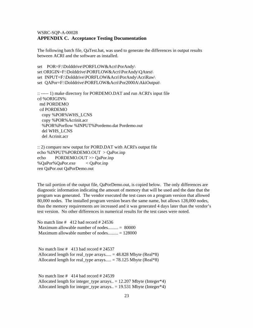
APPENDIX C. Acceptance Testing Documentation The following batch file, QaTest.bat, was used to generate the differences in output results between ACRI and the software as installed. set POR=F:\Dolddrive\PORFLOW&Acri\PorAndy\ set ORIGIN=F:\Dolddrive\PORFLOW&Acri\PorAndy\QAtest\ set INPUT=F:\Dolddrive\PORFLOW&Acri\PorAndy\AcriRaw\ set QAPor=F:\Dolddrive\PORFLOW&Acri\Por2000A\AkiOutput\ :: ----- 1) make directory for PORDEMO.DAT and run ACRI's input file cd %ORIGIN% md PORDEMO cd PORDEMO copy %POR%WHS_LCNS copy %POR%Acrinit.acr %POR%Porflow %INPUT%Pordemo.dat Pordemo.out del WHS_LCNS del Acrinit.acr :: 2) compare new output for PORD.DAT with ACRI's output file echo %INPUT%PORDEMO.OUT > QaPor.inp echo PORDEMO.OUT >> QaPor.inp %QaPor%QaPor.exe < QaPor.inp ren QaPor.out QaPorDemo.out The tail portion of the output file, QaPorDemo.out, is copied below. The only differences are diagnostic information indicating the amount of memory that will be used and the date that the program was generated. The vendor executed the test cases on a program version that allowed 80,000 nodes. The installed program version bears the same name, but allows 128,000 nodes, thus the memory requirements are increased and it was generated 4 days later than the vendor’s test version. No other differences in numerical results for the test cases were noted. No match line # 412 bad record # 24536 Maximum allowable number of nodes......... = 80000 Maximum allowable number of nodes......... = 128000 No match line # 413 bad record # 24537 Allocated length for real_type arrays..... = 48.828 Mbyte (Real*8) Allocated length for real_type arrays..... = 78.125 Mbyte (Real*8) No match line # 414 bad record # 24539 Allocated length for integer_type arrays.. = 12.207 Mbyte (Integer*4) Allocated length for integer_type arrays.. = 19.531 Mbyte (Integer*4)

WSRC-SQP-A-00028

24

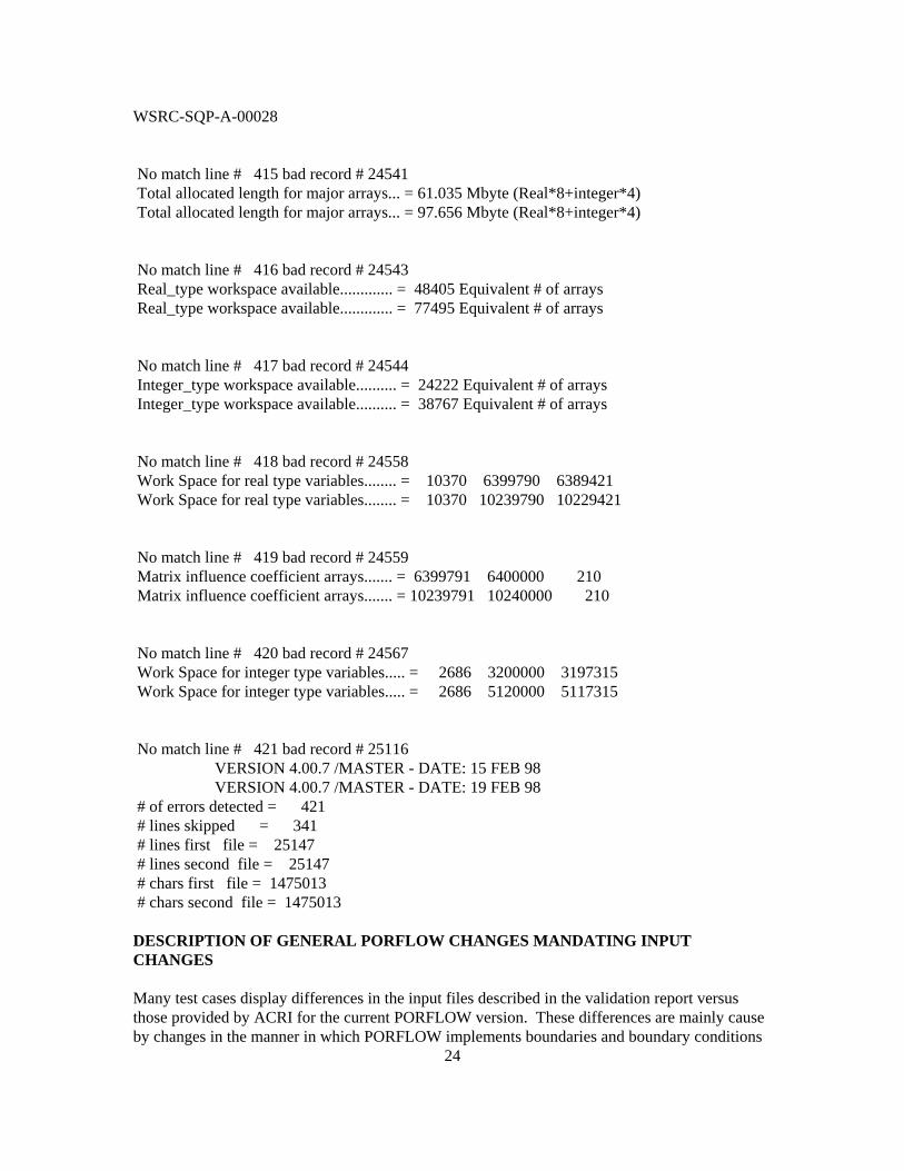
No match line # 415 bad record # 24541 Total allocated length for major arrays... = 61.035 Mbyte (Real*8+integer*4) Total allocated length for major arrays... = 97.656 Mbyte (Real*8+integer*4) No match line # 416 bad record # 24543 Real_type workspace available............. = 48405 Equivalent # of arrays Real_type workspace available............. = 77495 Equivalent # of arrays No match line # 417 bad record # 24544 Integer_type workspace available.......... = 24222 Equivalent # of arrays Integer_type workspace available.......... = 38767 Equivalent # of arrays No match line # 418 bad record # 24558 Work Space for real type variables........ = 10370 6399790 6389421 Work Space for real type variables........ = 10370 10239790 10229421 No match line # 419 bad record # 24559 Matrix influence coefficient arrays....... = 6399791 6400000 210 Matrix influence coefficient arrays....... = 10239791 10240000 210 No match line # 420 bad record # 24567 Work Space for integer type variables..... = 2686 3200000 3197315 Work Space for integer type variables..... = 2686 5120000 5117315 No match line # 421 bad record # 25116 VERSION 4.00.7 /MASTER - DATE: 15 FEB 98 VERSION 4.00.7 /MASTER - DATE: 19 FEB 98 # of errors detected = 421 # lines skipped = 341 # lines first file = 25147 # lines second file = 25147 # chars first file = 1475013 # chars second file = 1475013 DESCRIPTION OF GENERAL PORFLOW CHANGES MANDATING INPUT CHANGES Many test cases display differences in the input files described in the validation report versus those provided by ACRI for the current PORFLOW version. These differences are mainly cause by changes in the manner in which PORFLOW implements boundaries and boundary conditions

WSRC-SQP-A-00028

25

and minor adjustments in how the data are displayed, such as how often diagnostic information is displayed. PORFLOW uses free-form input that permits documentation to appear with the actual input data, hence, changes in documentation will not affect numerical results. PORFLOW modified its boundaries after Version 2.5 that was used in the validation report. For Version 2.5 the boundary nodes for PORFLOW (a finite difference code) were located outside the physical boundary of the model. If the physical boundary started at a coordinate of 0 and the next cell boundary was at a coordinate of 1, then the first cell node would be at 0.5 and the boundary node would be at –0.5. PORFLOW would calculate the physical boundary coordinate at the point midway between the first two nodes (one-half of –0.5 and 0.5). In later versions of PORFLOW the location of the boundary node was changed to align with the physical boundary of the model, or in this case at 0. Locations of the boundary nodes changed all around the physical boundary, both on the low side and the high side. This change allowed the user to specify the number of cell nodes, then input the corners of the mesh in a manner identical to that for a finite element code. Later versions of PORFLOW also modified how the sides of a model were defined for boundary conditions. Version 2.5 used –1 for the negative X direction (at the left-hand side of the model) and +1 for the positive X direction (at the right-hand side of the model), etc. Later versions replaced the “-1” with “X-“ and “+1” with “X+”, etc. To handle boundary conditions more naturally for unstructured grids, PORFLOW changed flux conditions from the sign indicating the direction of the flux to a positive sign indicating flux into the model and a negative sign indicating an outward flux. This sign convention does not apply to Dirichlet boundary conditions, such as when the pressure or concentration is set to a specific value. The sign convention is moot when the flux is zero. For the gradient boundary condition the older PORFLOW versions had the user specify the gradient in the opposite direction of the desired flux. Newer versions adopt the same sign convention as the flux boundary condition, namely that a positive value generates a positive flux into the physical model. The change in the flux sign convention produces changes according to the following table. Table 1. Sign Convention for Flux Boundary Conditions Boundary Old Sign New Sign Comments Lower Negative Negative Left, outward Lower Positive Positive Right, inward Upper Negative Positive Left, inward Upper Positive Negative Right, outward The change in the gradient sign convention produces changes according to the following table. Table 2. Sign Convention for Gradient Boundary Conditions

WSRC-SQP-A-00028

26

Boundary Old Sign New Sign Comments Lower Negative Positive Right, inward Lower Positive Negative Left, outward Upper Negative Negative Right, outward Upper Positive Positive Left, inward These two tables show between the old and new PORFLOW versions that the flux boundary conditions are switched at the upper boundaries, while the gradient boundary conditions are switched at the lower boundaries. DESCRIPTION OF APPLICABLE VERIFICATION AND BENCHMARK TEST CASES Each test case that directly affects the use of PORFLOW at SRS is described below. Of special interest are those test cases that include the flow of water in the vadose zone and the aquifer and the transport of contaminants by diffusion and advection. Given the above-stated PORFLOW changes and the requisite changes in the input files, each applicable verification and benchmark test case will be described in further detail. Verification Test Cases The verification cases are generally simple and can be compared to analytic solutions. Verification Test Case 3 Verification Test Case 3 examines the Theis solution for transient drawdown. On the GRID command line the descriptor NODES was added. This ensures that the numbers on the command are interpreted as nodes rather than corners and provides consistency between old and new versions of PORFLOW. This descriptor appears throughout most of the test cases and will not be discussed further. The first node was moved from 0.0 to 0.25 (halfway between the original 0.0 and 0.50) but the last node at 2000 was not moved to 1900.0 (halfway between the original 1800.0 and 2000.0). This likely caused little change in the results and it is unknown which, if either set of input is accurate. On the BOUNDARY command line for Y, the “-2” was replaced by “Y-“ as required. The DIAGNOSTIC and OUTPUT commands were changed with no impact on actual results, because the key information was saved in the archive file, “V3.ARC.” Verification Test Case5 Verification Test Case 5 involves coupled flow and heat transfer in a regional flow system. While isothermal models are typically executed at SRS, results from a nonisothermal case that involves flow is applicable in that it demonstrates that the flow portion operates correctly. For this test case the number of nodes was increased from 41 by 41 to 42 by 42. Rather than specifying the location for each node, the RANGE command was used as a substitute. These

WSRC-SQP-A-00028

27

develop an identical model, except that in the second case the mesh is finer. Of possible concern would be the location of sources, however, only boundary conditions are applied. The boundary conditions changed according to the convention of “-1” changing to “X-“, etc. The nonzero gradient for temperature at the lower Y boundary correctly switched signs. Finally, some of the output specifications were modified. Verification Test Case6 Verification Test Case 6 involves three-dimensional transport of a contaminant, which is very important to SRS modeling. It consists of a homogeneous, isotropic medium with an infinite horizontal source on the upper surface and a constant horizontal flow. This case very closely mimics most aquifer cases developed at SRS, except that the more complex subsurface consisting of multiple material types is lacking. For this case, both sets of input coordinates are consistent, but are slightly incorrect. The extent of the X-direction is described as being 3700 m long. The coordinates ranged from –700 to 3000 in both cases. However, they are node locations by default for the older PORFLOW version and are node locations in the newer PORFLOW version by the NODE descriptor (corners are the default), rather than the desired corner locations. Similarly the extent of the Y-direction is described as being 800 m long. The original node coordinates ranged from –10 to 800. This placed the lowest node in the range at the correct location because the corner of the physical model would be at zero, halfway between –10 and +10 for the first and second nodes. However the upper corner would be at 745, halfway between the 800 and the 690 of the next to highest node in the range. The more recent data set extends from 0 to 800 but it specifically calls out the data as nodes, which is incorrect because it should have been corner data. The extent of the Z-direction is described as 56 m. The original data ranged from -56 to 0.05. Only the upper node is at the correct location because the corner would be at zero, halfway between –0.05 and +0.05. The new data ranges from –50 to 0 as nodes. This is incorrect because the lower location has been changed from –56 to –50. The boundary conditions are set to zero flux at all boundaries except the lower X boundary where the concentration is set to zero. This caused the input line to be changed from “-1” to “X-“. However, PORFLOW changed the definition of the flux condition on a boundary command. Originally the flux option meant that advection could still move contaminants across the boundary, but in the more recent PORFLOW versions, even this is prevented. Typically contaminants are transported to a boundary but cannot penetrate it, thus they rapidly accumulate at the boundary. If only results in the interior of the model are important, then this effect is minor only affecting the mass balance. The geometric property was omitted in the newer version, thus the calculation of the properties of the host porous matrix at the element interface would default to the harmonic mean. Integration of the concentration by the CONDIF approach was omitted in the newer version. The CONDIF approach as described in Runchal, 1997 is provided below.

WSRC-SQP-A-00028

28

“The numerical integration starts with the assumption of an integration profile for the state variable. Two different kinds of profiles are employed. These are the first- and second-order polynomial profiles and the exponential profile. These integration profiles result, respectively, in the ‘upwind’, and the central difference and, the exponential schemes. The first two are schemes combined in a hybrid scheme. The central difference scheme, which provides second-order accuracy, is the preferred scheme. However, use of the central difference scheme may result in numerical instabilities if the magnitude of the local value of the grid Peclet number exceeds 2. With U, δL and Γ, respectively, as the velocity component, grid interval and diffusivity in a given direction, the grid Peclet number, Pe, is defined as:

Pe = U δL / Γ. (4.2.1) The local value of the Peclet number at each grid node is constantly monitored in each direction. If Pe > 2, then the numerical scheme automatically shifts to the ’upwind’ formulation. This method of enhancing stability is known as the hybrid scheme (Runchal, 1972). The hybrid scheme has second-order accuracy if the Pe < 2; otherwise, it is only first-order accurate. Because upwinding results in an increasing amount of numerical diffusion as the angle between the velocity vector and the grid lines increases, PORFLOWTM allows the use of an exponential numerical scheme (Spalding, 1972) to represent the exact solution of the one-dimensional form of transport equations without sources. Th eexponential scheme cannot be accurately classified; however, in practice, it is known to decrease numerical dispersion if the flow is primarily unidirectional and source terms are small. Otherwise, its accuracy is comparable to that of the hybrid scheme. An alternate method to obtain numerical stability with second-order accuracy is that of the CONDIF scheme (Runchal, 1987b) which is a modified central-difference scheme. It is a second-order member of the TVD family of numerical schemes (Harten, 1983) that leads to an unconditionally stable formulation. A third option which is available is that of a version of the QUICK scheme (Leonard, 1979) which has been adapted for nonorthogonal grids. The user controls the method of evaluation of the integrals, which is equivalent to the selection of a ‘basis function’ in the finite-element technique. For most problems, the hybrid scheme is sufficient. If the grid is very coarse, then the CONDIF or the QUICK scheme should be employed. “ ACRI, 1994 states:

“The maximum Peclet number for the grid employed is 5.5 and the maximum Courant number is 0.04. Since the Peclet number is almost three times the desired value of 2, some numerical errors may be present. These results could be improved by smaller grid size.”

Personal communication with Runchal indicated that results from the newer PORFLOW version were in close agreement with earlier results. Thus, in spite of removing the CONDIF control that helps compensate for a coarse grid the results were quite reasonable. The text states that the problem is symmetric in the lateral (y) direction, hence only half the domain was simulated. The text and the figure show a domain of 800 m with the source in the center. If only half the domain in the y direction were modeled, the model would encompass only

WSRC-SQP-A-00028

29

400 m, but the input file encompasses 800 m, thus the text and the input file are inconsistent. No original convergence criteria were specified thus it defaulted to 0.001. The revised convergence was 1.E-7, which is much tighter. Minor changes to the diagnostics, history and output selections were noted. The solution originally was set to about 1.58E8 seconds in uniform steps of about 3.15E4 seconds. The revision started with steps of 2.E3 seconds that increased to a maximum of 5E6 seconds. These are all subjective. While the magnitude of the Courant number would increase, if the problem has stabilized by the time it becomes large, there should be minimal effect on the final results. Verification Test Case7 Verification Test Case 7 involves Philip’s horizontal unsaturated flow case where a wetting front is initiated by a pressure change at one boundary. Primarily, only minor changes were noted in the GRID command, and adjusting the BOUNDARY command, the DIAGNOSTIC command and the OUTPUT command. The extent in the X-direction should be 20 cm, but because node locations are used the actual extent of the physical model is shortened slightly. Verification Test Case8 Verification Test Case 8 involves Philip’s vertical unsaturated column that is similar to the Philip’s horizontal column, but the column is vertical so that capillary and gravity forces can take effect. In both cases the range for the Y coordinate is set to 15 cm. In the original version of PORFLOW, the default was for nodes, which generated a slightly shorted physical domain. In the newer PORFLOW version, the default is for corners, which matches the physical domain with the text. Minor changes are apparent in that the order of some commands has changed, the BOUNDARY input has been modified and the DIAGNOSTIC and OUTPUT commands have been adjusted. Verification Test Case9 Verification Test Case 9 involves steady-state infiltration from a line source to a water table. This case involves modeling the vadose zone with the water table as its lower boundary, similar to the vadose zone modeling at SRS. Here the coordinates are specified by the range option. The range option in the original PORFLOW version used corners rather than nodes as the default (contrary to statements in the user’s manual). Both data sets for coordinates are correct. Minor changes to the GRID command, BOUNDARY commands, the DIAGNOSTIC command and the OUTPUT command were noted between the two sets of input files. The boundary condition for the pressure at the Y- face changed from “interface” to “value.” The original PORFLOW allowed the user to prescribe a value at the node with “value” or a value at the element interface, i.e., at the edge of the physical model with “interface.” Because the newer version of PORFLOW moves the location of the boundary node to the edge of the physical model, the “value” and the “interface” are synonymous and are equivalent to the previous “interface.” “Interface” has been omitted from the newer PORFLOW, so older input sets that relied on the “value” may produce different results if used with the newer PORFLOW. The relation between the pressure and the saturation is expressed as a Brooks & Corey

WSRC-SQP-A-00028

30

relationship in the original data set, but as an exponential relationship in the subsequent data set. For a steady-state solution the difference apparently has minimal effect on the final results. Verification Test Case10 Verification Test Case 10 involves free-surface Boussinesq flow with recharge from one side in a semi-infinite, unconfined aquifer. The extent of the model in the X-direction is 200 m. Both data sets employ a minimum and maximum for the X that apparently properly describes the physical model. However, the earlier version of PORFLOW used a default of nodes, thus the physical model would have been slightly smaller than the defined model. The Y-direction had an extent of 11 m. The original model prescribed nodes that extended from 0 to 11.1. The physical boundaries would have been from 1 to 11, or only 10 m in extent. The more recent data set prescribes nodes from 0 to 11, and because the boundary nodes in the later PORFLOW are aligned with the physical model boundaries this prescription is correct. Initial conditions were originally prescribed with the INITIAL command. The more recent version uses a combination of the SET command and a BOUNDARY command with the same effect. The convergence is tightened from 1E-6 to 1E-10 in the later data set, although the maximum number of iterations is reduced from 1000 to 25 producing a tradeoff. The BOUNDARY command, DIAGNOSTIC command and the OUTPUT command are modified. The DIAGNOSTIC command is misspelled as DIAGNOSITC in both versions, but PORFLOW only relies on the first four characters, thus the operation of the model will not be affected. Verification Test Case11 Verification Test Case 11 involves free-surface Boussinesq flow with seepage from the surface in an unconfined aquifer. All the comments for Verification Test Case 10 apply here. Benchmark Test Cases The benchmark test cases produce solutions that are compared to solutions from other computer codes, because typically the cases are too complex to afford analytic solutions. All the test cases “have been used previously for validation of other computer codes” (ACRI, 1994). Having test cases that were important enough to use for validation of other computer codes indicates that they are excellent candidates for the PORFLOW validation. Benchmark Test Case1 Benchmark Test Case 1 involves two-dimensional transient infiltration. The model size is described as being 15 cm in the X-direction and 10 cm in the Y-direction. The original data set provided a minimum and a maximum for the X-direction as 0 and 0.15 m. Given the default of nodes, the size of the physical domain would be slightly short, by 0.01 m. The Y coordinate was described as a range of 0.1 m, which would be correct. For the later PORFLOW version, because the boundary nodes are aligned with the edge of the physical model, the same BOUNDARY commands with the NODE modifier produce a correct model.

WSRC-SQP-A-00028

31

Other minor changes are found in the BOUNDARY command, the DIAGNOSTIC command and the OUTPUT command. Output results were compared with results from the TOUGH computer program. Benchmark Test Case2 Benchmark Test Case 2 involves two-dimensional steady-state infiltration. The model size is 150 m in the X direction and 35 m in the Y direction (the figure shows a Y range of 42 m). The original data set had a range in the X coordinate from 0 to 150 for the nodes. It would have ranged from 2.5 to 147.5 for the physical model or only 145 m, rather than the intended 150 m. The Y coordinate ranged from –0.1 to 36 for the nodes. The range for the physical model would have been 0 to 35, which was correct. The newer data set defined ranges that were correct. The newer data set increased the number of nodes in the X-direction from 31 to 32. This helped align the corners (or cell faces) at 5 m intervals. The number of nodes in the Y-direction remained at 33. The original data set had distances between node locations that varied from 0.2 m to 2 m to provide better resolution near the location of the phreatic surface. Specifying a range forces all distances to equal values and that resolution is lost. The older version specified a datum of 0,0 while none was specified for the newer data set, but because the defaults are zero these are equivalent. The BOUNDARY commands were changed to reflect the new format. The boundary condition along the upper X boundary was correctly applied by increasing the location from 31 to 32 that matched the number of nodes in the X direction. The boundary condition at Y+ was a flux of –1 in the original (downward) and +1 in the newer data set (into the domain which is downward). The convergence criterion was loosened from 1E-5 to 1E-3 with a maximum iteration count changed from a default of 100 to 500. The original data set required that the problem be solved for 4 years while the late data set required a steady state solution. As long as a satisfactory solution is achieved, the convergence criterion difference is not important. The output region for the newer data set was selected for nodes 1,1 to 999,999 with an interval of 2,2. This allowed half of the data to be skipped. PORFLOW allows the 999,999 upper limit even though the size of the problem domain is only 32 by 33. The results from this test case were compared with FEMWATER results. Benchmark Test Case3 Benchmark Test Case 3 is a simulation of the Jornada Test Trench in an extremely dry heterogeous soil. The area was heavily instrumented and infiltration experiments were conducted. This case qualifies both as a validation case and as a short-term field validation case. Because the SRS site is a much wetter site the value of the field validation is limited. However, it is much more difficult to simulate extremely dry conditions thus this is a challenging test case. The extent of the model is 800 cm in the X direction and 650 cm in the Y direction. The original data set had a range of X-direction nodes from –5 to 820 and X-direction corners from 0 to 800

WSRC-SQP-A-00028

32

that properly described the physical model. Similarly the range of Y-direction nodes was from -655 to 5 and X-direction corners from –650 to 0. The newer data set took advantage of the boundary nodes’ locations at the edge of the physical boundary and placed the lower and upper nodes at the proper locations of 0 and 800 for the X direction and –650 and 0 for the Y direction. The BOUNDARY commands were modified to conform to the new convention. The flux for the pressure equation at the upper Y boundary was a –2 cm/day in the original data set (downward) while in the newer data set it was +2 cm/day (inward), but it is also downward. The DIAGNOSTIC command was modified to report less often and its location was moved. Two convergence criteria were provided in the newer data set, but none in the original data set. One CONVERGENCE command is for FLOW that is not described in either user’s manual, although an example is provided in the newer user’s manual. The CONVERGENCE command for pressure in the newer data set is equivalent to the default criterion. This benchmark case was compared to results from the FLASH code and the TRACER3D code. CONCLUSIONS OF VALIDATION TESTING PORFLOW has been tested previously by international experts such as Allan Freeze and by the Southwest Research Center for the Nuclear Regulatory Commission (Collard,1998). The high level of testing by experts and the extensive test cases provided by the author, most of which are applicable, indicates that PORFLOW can be readily applied for SRS problems with the expectation of correct program performance. Some of the problems for which PORFLOW has been validated are as follow:

• Vadose zone flow problems with multiple soil types • Vadose zone contaminant transport problems with multiple soil types and simple

chemistry • Aquifer flow problems with multiple soil types • Aquifer contaminant transport problems with multiple soil types and simple

chemistry. Cases with contaminant sources were documented. Multiphase and nonisothermal cases were not documented. For problems that are simple extensions of previous problems, such as examining an additional nuclide, the PI need do no further testing. For new problems, the PI should review the test cases that were documented to see if they adequately address the requirements for the new problem. If previous test cases are sufficient, then the PI should document that fact with some justification. If previous test cases are not sufficient, then the PI should execute new test cases and document the results either before modeling the new problem, or in parallel with the new problem, although there is some risk in performing both in parallel.

WSRC-SQP-A-00028

33

APPENDIX D. Sample Batch File for Executing PORFLOW The sample batch file executes PORFLOW using an input file named “run.dat” and creates an output file named “run.out.” set Por=F:\Dolddrive\PORFLOW&Acri\PorAndy\ if not Exist Acrinit.acr copy %Por%Acrinit.acr if not Exist WHS_LCNS copy %Por%WHS_LCNS %Por%Porflow run.dat run.out del Acrinit.acr del WHS_LCNS

WSRC-SQP-A-00028

34

DISTRIBUTION To: W.T. Goldston, 705-3C F.J. Riddle, Jr., 766-H

M.K. Harris, 773-42A J.J. Connelly 773-41A C.R. Mastromonico, 730-A G.P. Flach, 773-42A

W.E. Stevens, 773-A B.T. Butcher, 773-43A L.B. Collard, 773-43A J.R. Cook, 773-43A

E.L. Wilhite, 773-43A STI, 4 copies, 703-43A WPT File, 773-43A