wsp 2254 - usgs · these developments have both positive and negative effects on accuracy of the...

where R, is the ratio of isotopes measured in the sample and Rs~~D is the ratio of the same isotopes in the reference standard. The 6, value is in parts per thousand, commonly abbreviated “permil.”

The isotopes most extensively used in hydrology are deuterium (D or hydrogen-2) and oxygen-18. These are present in average proportions of 0.01 percent and 0.2 percent of hydrogen and oxygen, respectively. For hydrologic purposes, the reference standard composition is that of average seawater (SMOW, standard mean ocean water), and relative enrichment or impoverishment of the isotope in water samples is expressed as a 62H or al80 departure above or below SMOW=O, in parts per thousand. Compared with deuterium, the radioactive isotope”H (tritium) is extremely rare. Even in the higher concentrations observed in rainfall in the United States from 1963 to 1965 (Stewart and Farnsworth, 1968), the abundance of tritium seldom reached as much as 1 tritium atom for each 10” atoms of hydrogen. This is some 10 orders of magnitude below the abundance of deuterium. Deuterium and “0 are of particular hydrologic significance because they produce a significant proportion of molecules of Hz0 that are heavier than normal water. In the process of evaporation, the heavier molecules tend to become enriched in residual water, and the lighter species are more abundant in water vapor, rain and snow, and most freshwater of the hydrologic cycle; the heavier forms are more abundant in the ocean.

Some of the early studies of deuterium and oxygen- 18 contents of water from various sources were made by Friedman (1953) and by Epstein and Mayeda (1953), and the usefulness of isotopic-abundance data in studies of water circulation has been amply demonstrated by subsequent applications. The abundance of the hydrogen isotopic species has been considered a useful key to deciding whether a water from a thermal spring contains a significant fraction of water of magmatic or juvenile origin that has not been in the hydrologic cycle previously (Craig, 1963).

Biological processes tend to produce some fractionation of isotopes. Among the studies ofthese effects is the paper by Kaplan and others (1960) relating to enrichment of sulfur-32 over sulfur-34 in bacterially reduced forms of the element, and the papers on fractionation of carbon- 12 and carbon-13, as in fermentation and other biologically mediated processes (Nakai, 1960) or in processes related to calcite deposition (Cheney and Jensen, 1965). Nitrogen isotopes 14N and ‘“N also can be fractionated biologically. Carbon-13 has been used in developing mass-balance models of ground-water systems (Wigley and others, 1978).

Summaries of this extensive field of research have been assembled by Fritz and Fontes (1980). The fractionation factors of stable isotopes that are of geochemical interest were compiled by Friedman and O’Neil(l977).

Fractionation effects are likely to be most noticeable in the lighter weight elements, as the relative differences in mass of isotopes is larger for such elements.

ORGANIZATION AND STlJDY OF WATER-ANALYSIS DATA

Hydrologists and others who use water analyses must interpret individual analyses or large numbers of analyses at the same time. From these interpretations final decisions regarding water use and development are made. Although the details of water chemistry often must play an important part in water-analysis interpretation, a fundamental need is for means of correlating analyses with each other and with hydrologic or other kinds of information that are relatively simple as well as scientifically reasonable and correct. It may be necessary, for example, in the process of making an organized evaluation in a summary report of the water resources of a region, to correlate water quality with environmental influences and to develop plans for management of water quality, control of pollution, setting of water-quality standards, or selecting and treating public or industrial water supplies.

The objective of this sec:tion is to present some techniques by which chemical analyses of waters can be used as a part of hydrologic investigations. One may reasonably suppose that geologic, hydrologic, cultural, and perhaps other factors have left their mark on the water of any region. Finding and deciphering these effects is the task that must be addressed. The procedures range from simple comparisons and inspection of analytical data to more extensive statistical analyses and the preparation of graphs and maps that show significant relationships and allow for extrapolation of available data to an extent sufficient to be most pra,ctical and useful.

The use of water-quality data as a tool in hydrologic investigations of surface- and ground-water systems often has been neglected. In appropriate circumstances, chemical data may rank with geologic, engineering, and geo- physical data in usefulness in the solution of hydrologic problems. Arraying and manipulating the data, as suggested in the following pages, may lead the hydrologist to insight into a problem that appears from other available information to be insoluble.

Perhaps the most significant development in the field of water-quality hydrology during the 1970’s was the increasing use of mathematical modeling techniques. Some consideration of this topic is essential here, although the discussion cannot cover the subject in detail (nor would it be useful to do so in view of probable future improvements in modeling techniques). The subject of mathematical modeling will be considered further in the section of this book entitled “Mathematical Simulations- Flow Models.”

162 Study and Interpretation of the Chemical Characteristics of Natural Water

Evaluation of the Water Analysis same set of procedures.

The chemical analysis, with its columns of concentration values reported to two or three significant figures accompanied by descriptive material related to the source and the sampling and preservation techniques, has an authoritative appearance which, unfortunately, can be misleading. Although mention has already been made of some of the effects of sampling techniques, preservation methods, and length of storage before analysis on the accuracy of results, it should be noted again that many completed analyses include values for constituents and properties that may be different from the values in the original water body. Many analyses, for example, report a pH determined in the laboratory; almost certainly, such pH values deviate from the pH at time of sampling. Roberson and others (1963) published some data on the extent of such deviations. The user of the analysis also should be concerned with the general reliability of all the analytical values, including those for constituents generally assumed to be stable.

Accuracy and Reproducibility

Increasing reliance on instrumental methods and automation has been necessary in most institutional laboratories to cope with increased workloads and to control costs. These developments have both positive and negative effects on accuracy of the product. Quality control must be emphasized continually. This is usually done by sub- mitting samples of known composition along with the samples of unknown composition. The Analytical Refer- ence Service operated by the U.S. Environmental Protec- tion Agency at its Taft Center laboratory in Cincinnati, Ohio, circulated many standard samples among cooper- ating testing laboratories that use these methods and observed many interesting and, at times, somewhat dis- concerting results. The results that have been published show that when the same sample is analyzed by different laboratories, a spread of analytical values is obtained that considerably exceeds the degree of precision most analytical chemists hope to attain. The need for quality control in the production of analytical data and in methods of evaluating and improving accuracy were summarized by Kirchmer (1983).

Under optimum conditions, the analytical results for major constituents of water have an accuracy of +2-+lO percent. That is, the difference between the reported result and the actual concentration in the sample at the time of analysis should be between 2 and 10 percent of the actual value. Solutes present in concentrations above 100 mg/L generally can be determined with an accuracy of better than -t5 percent. Limits of precision (reproducibility) are similar. For solutes present in concentrations below 1 mg/L, the accuracy is generally not better than +lO percent and can be poorer. Specific statements about accuracy and reproducibility have not been made for most of the analytical determinations discussed in this book because such statements are meaningful only in the context of a specific method and individual analyst. When concentrations are near the detection limit of the method used, and in all determinations of constituents that are near or below the micro- gram-per-liter level, both accuracy and precision are even more strongly affected by the experience and skill of the analyst.

Analytical errors are at least partly within the control of the chemist, and for many years efforts have been made to improve the reliability of analytical methods and instruments and to bring about uniformity in procedures. The majority of laboratories active in the water- analysis field in the United States use procedures described in “Standard Methods for Analysis of Water and Waste Water” (American Public Health Association and others, 1980) which is kept up to date by frequent revisions. Other manuals such as those of the U.S. Geological Survey (Skougstad and others, 1979) specify much the

Lishka and others (1963) summarized results of several Analytical Reference Service studies in which the spread in analytical values reported by different laboratories for the same sample were pointed out. For example, of 182 reported results for a standard water sample, 50 percent were within +6 mg/L of the correct value for chloride (241 mg/L). The standard deviation reported for this set of determinations was 9.632 mg/L. If these results are evaluated in terms of confidence limits, or probability, assuming a normal distribution, the conclusions may be drawn that a single determination for chloride in a sample having about 250 mg/L has an even chance of being within f6 mg/L of the correct value and that probability is 68 percent that the result will be within f9.6 mg/L of the correct value. The probability of the result being within +20 mg/L of the correct value is 95 percent. The results for other determinations reported by Lishka and others were in the same general range of accuracy. Before the statistical analysis was made, however, Lishka and others rejected values that were grossly in error. The rejected determinations amounted to about 8 percent of the total number of reported values. The probable accuracy would have been poorer had the rejected data been included, but it may not be too unreal- istic to reject the grossly erroneous results. In practice, the analytical laboratory and the user of the results will often be able to detect major errors in concentration values and will reject such results if there is some prior knowledge of the composition of the water or if the analysis is reasonably complete. Methods of detecting major errors will be described later.

The results of a single analyst or of one laboratory should have somewhat lower deviations than the data

Significance of Properties and Constituents Reported in Water Analyses 163

cited above. It would appear, however, that the third significant figure reported in water analysis determinations is usually not really meaningful and that the second figure may in some instances have a fairly low confidence limit. In the data cited by Lishka and others, there is only a 5-percent chance that a chloride determination in this range of concentration would be as much as 10 percent in error. The effects of sampling and other nonanalytical uncertainty are excluded from this consideration.

Quality-control programs for U.S. Geological Sur- vey water-analysis laboratories and laboratories of its contractors and cooperators use standard reference samples that are analyzed by all participants. Results of these analyses are released to all the laboratories taking part. Quality-assurance practices in U.S. Geological Survey investigations were described by Friedman and Erdmann (1983).

Results of an international study in which 7 water samples were analyzed by 48 different laboratories in 18 countries were reported by Ellis (1976). These results led Ellis to conclude (p. 1370): “While progress has been made in recent years in improving the standard of trace element analysis, in many laboratories the standard of water analysis for many common constituents still leaves much to be desired.” The 95-percent confidence range for major constituents in Ellis’ study was generally similar to that of Lishka and others (1963).

It should also be noted that in the interlaboratory studies described by Lishka and others (1963) and by Ellis (1976) the laboratories participating were aware of the special nature of the samples involved and may have given them somewhat better than routine treatment. Internal quality control practices for analytical laboratories (Friedman and Erdmann, 1983) generally utilize “blind” samples of known composition, submitted without being identified in any special way.

Organizations in Federal and State governments and other laboratories that publish analyses intended for general purposes use accuracy standards that are generally adequate for the types of interpretation to be discussed in this section of this book. The personnel at all such organizations, however, share human tendencies toward occasional error. A first consideration in acceptance of an analysis is the data-user’s opinion of the originating laboratory’s reputation for accuracy of results, and perhaps its motivation for obtaining maximum accuracy. Data obtained for some special purposes may not be satisfactory for other uses. For example, some laboratories are concerned with evaluating water for conformity to certain standards and may not determine concentrations closely if they are far above or far below some limiting value. Accuracy Checks

The accuracy of major dissolved-constituent values

in a reasonably complete chemical analysis of a water sample can be checked by calculating the cation-anion balance. When all the major anions and cations have been determined, the sum of the cations in milliequivalents per liter should equal the sum of the anions expressed in the same units. If the analytical work has been done carefully, the difference between: the two sums will generally not exceed 1 or 2 percent of the total of cations and anions in waters of moderate concentration (250-1,000 mg/L). If the total of anions and cations is less than about 5.00 meq/L, a somewhat larger percentage difference can be tolerated. If an analysis is found acceptable on the basis of this check, it can be assumed there are no important errors in concentrations reported for major constituents.

Water having dissolved-solids concentrations much greater than 1,000 mg/L tends to have large concentrations of a few constituents. In such water, the test of anion-cation balance does not adequately evaluate the accuracy of the values of the lesser constituents.

The concept of equivalence of cations to anions is chemically sound, but in some waters it may be difficult to ascertain the forms of some of the ions reported in the analysis. To check the ionic balance, it must be assumed that the water does not contain undetermined species participating in the balance and that the formula and charge of all the anions or cations reported in the analysis are known. Solutions that are strongly colored, for example, commonly have organic anions that form complexes with metals, and the usual analytical procedures will not give results that can be balanced satisfactorily.

The determination of alkalinity or acidity by titration entails assumptions about the ionic species that may lead to errors. The end point of such a tritration is best identified from a titration curve or a derivative curve

(Barnes, 1964). The use of fixed pH as the end point can lead to errors. Some ions that contribute to alkalinity or acidity may be determined specifically by other procedures and can thus appear in the ionic balance twice. For most common types of natural water this effect will not be significant. Water having a pH below 4.50 presents analytical problems because, as noted in the discussion of acidity earlier in this book, the titration is affected by several kinds of reactions and may not provide a value that can be used in reaching an ionic balance.

Many analyses that were made before about 1960 reported computed values for sodium or for sodium plus potassium. These values were obtained by assigning the difference between milliequivalents per liter of total anions determined and the sum of milliequivalents per liter of calcium and magnesium. Obviously, such an analysis cannot be readily checked for accuracy by cation-anion balance. Although calculated sodium concentrations are not always identified specifically, exact or nearly exact agreement between cation and anion totals for a series of


analyses is a good indication that sodium concentrations were calculated. Modern instruments have greatly simplified the determination of alkali metals, and analyses with calculated values are no longer common.

Another procedure for checking analytical accuracy that is sometimes useful is to compare determined and calculated values for dissolved solids. The two values should agree within a few milligrams or tens of milligrams per liter unless the water is of exceptional composition, as noted in the discussion of these determinations earlier in this book. The comparison is often helpful in identifying major analytical or transcribing errors.

An approximate accuracy check is possible using the conductivity and dissolved-solids determinations. The dissolved-solids value in milligrams per liter should generally be from 0.55 to 0.75 times the specific conductance in micromhos per centimeter for waters of ordinary composition, up to dissolved-solids concentrations as high as a few thousand milligrams per liter. Water in which anions are mostly bicarbonate and chloride will have a factor near the lower end of this range, and waters high in sulfate may reach or even exceed the upper end. Waters saturated with respect to gypsum (analysis 3, table 15, for example) or containing large concentrations of silica may have factors as high as 1.0. For repeated samples from the same source, a well-defined relationship of conductivity to dissolved solids often can be established, and this can afford a good general accuracy check for analyses of these samples. The total of milliequivalents per liter for either anions or cations multiplied by 100 usually agrees approximately with the conductivity in micromhos per centimeter. This relationship is not exact, but it is somewhat less variable than the relationship between conductivity and dissolved solids in milligrams per liter. The relationship of dissolved solids to conductance becomes more poorly defined for waters high in dissolved solids (those exceeding about 50,000 mg/L) and also for very dilute solutions, such as rainwater, if the nature of the principal solutes is unknown. For solutions of well-defined composition such as seawater, however, conductivity is a useful indicator of ionic concentration.

A simple screening procedure for evaluating analyses for the same or similar sources is to compare the results with one another. Errors in transcribing or analytical error in minor constituents containing factors of 2 or 10 sometimes become evident when this is done. It is common practice, however, to make this type of scrutiny before data are released from the laboratory, and it is most useful to do it before the sample is discarded so that any suspect values can be redetermined.

Analyses reporting calculated zero values for sodium or indicating sodium concentration as less than some round number commonly result from analytical errors causing milliequivalents per liter for calcium and magnesium to equal or exceed the total milliequivalents per

liter reported for anions; thus, there is nothing to assign to sodium for calculation purposes. A zero concentration for sodium is rarely found if the element is determined.

Certain unusual concentration relationships among major cations can be considered as grounds for suspicion of the analysis’ validity. A zero value for calcium when more than a few milligrams per liter are reported for magnesium, or a potassium concentration substantially exceeding that of sodium unless both are below about 5 mg/L, are examples. This is not to say that waters having these properties do not exist. They are rare, however, and should be found only in systems having unusual geochemical features.

Groups of analyses from the same or similar sources in which all magnesium concentrations are similar but calcium concentrations have a rather wide range may indicate that calcium and bicarbonate were lost by pre- cipitations of calcium carbonate. This can occur in water- sample bottles during storage and also in the water- circulation system before sampling.

Significant Figures

Water analyses in which concentrations in milligrams per liter are reported to four or five significant figures are commonly seen. The notion of high accuracy and precision conveyed by such figures is misleading, because ordinary chemical analytical procedures rarely give better than two-place accuracy. Usually, the third significant figure is in doubt, and more than three is entirely superfluous. Analytical data in terms of milliequivalents per liter in the tables in this book were calculated from the original analytical data in mg/L. They are routinely carried to two or three decimal places but are not accurate to more significant figures than the mg/L values.

A concentration of 0 mg/L reported in chemical analyses in this book should be interpreted as meaning that the amount present was less than 0.5 mg/L and that the procedure used could not detect concentrations less than 0.5 mg/L. Concentrations of 0.0 or 0.00 mg/L imply lower detection limits. Some analysts report such findings in terms such as “<0.05 mg/L” when the figure given is the detection limit. These values should not be interpreted as indicating that any specific concentrations of the element was present. Other authors may use different conventions.

General Evaluations 06 Areal Water Quality

The type of water-analysis interpretation most commonly required of hydrologists is preparation of a report summarizing the water quality in a river, a drainage basin, or some other area1 unit that is under study. The writer of such a report is confronted with many difficulties. The chemical analyses with which the writer must work

Organization and Study of Water-Analysis Data 165

usually represent only a few of the water sources in the area and must be extrapolated. The finished report must convey water-quality information in ways that will be understandable both to technically trained specialists and to interested individuals less familiar with the field. Conclusions or recommendations relating to existing conditions or to conditions expected in the future are usually required.

As an aid in interpreting groups of chemical analyses, several approaches will be cited that can serve to relate analyses to each other and to provide means of extrapolating data areally and temporally. Different types of visual aids that are useful in reports will be described. The basic methods considered are inspection and simple mathematical orstatistical treatment to bring out resemblances among chemical analyses, procedures for extrapolation of data in space and time, and preparation of graphs, maps, and diagrams to show the relationships developed.

The final product of many hydrologic studies is now expected to be a mathematical model that can relate observable effects to specific causes and can provide a basis for predicting quantitatively the future behavior of the system studied.

Mathematical modeling of water quality is commonly thought of as representing the application of the modern electronic computer in the field of chemical hydrology. It is clear, however, that the principles on which such models are designed and the application of these principles through relationships of physics and chemistry for quantitative prediction of solute behavior are not new. The computer has made such applications simpler and more practicable. Its ability to solve complex problems holds bright promise for future applications.

Inspection and Comparison

The first step in examining water analyses, after accepting their reliability, is generally to group them by hydrologic or geologic categories, as appropriate. After this has been done, simple inspection of a group of chemical analyses generally will make possible a separa- tion into obviously interrelated subgroups. For example, it is easy to group together the waters that have dissolved- solids concentrations falling within certain ranges. The consideration of dissolved solids, however, should be accompanied by consideration of the kinds of ions present as well.

A common practice in literature on water quality is to refer to or classify waters by such terms as “calcium bicarbonate water” or “sodium chloride water.” These classifications are derived from inspection of the analysis

and represent the predominant cation and anion, expressed in milliequivalents per liter. These classifications are meant only to convey general information and cannot be expected to be precise. They may, however, be somewhat misleading if carelessly applied. For example, a water ought not be classed as a s’odium chloride water if the sodium and chloride concentrations constitute less than half the total of cations and anions, respectively, even though no other ions exceed them. Water in which no one cation or anion constitutes as much as 50 percent of the totals should be recognized as a mixed type and should be identified by the names of all the important cations and anions.

Ion Ratios and Water Types

Classifications of the type just described are only rough approximations, and for most purposes in the study of chemical analyses a more exact and quantitative procedure is required. Expression of the relationships among ions, or of one constituent to the total concentration in terms of mathematical ratios, is often helpful in making resemblances and differences among waters stand out clearly. An example of the use of ratios is given in table 21, in which three hypothetical chemical analyses are compared. All three analyses could be considered to represent sodium bicarbonate waters, and they do not differ greatly in total concentration. The high proportion of silica in waters B and C, their similiar Ca:Mg and Na:Cl ratios, and their similiar proportions of SO4 to total anions establish the close similarity of B and C and the dissimilarity of both to A. For most comparisons of this type, concentration values expressed in terms of milliequivalents per liter or moles per liter are the more useful, although both gravimetric and chemically equivalent units have been used. Data in the latter form show more directly the sort of 1: 1 ionic relationship that would result if solid NaCl were being dissolved.

The data in table 21 are synthetic, and actual analyses often do not show such well-defined relationships. Ratios are obviously useful, however, in establishing chemical similarities among waters, for example, in grouping analyses representing a single geologic terrane, or a single aquifer, or a water-bearing zone. Fixed rules regarding selection of the most significant values to compare by ratios cannot be given, but some thought as to the sources of ions and the chemical behavior that might be expected can aid in this selection. The ratio of silica to dissolved solids may aid in identifying water influenced by the solution of silicate minerals, and the type of mineral itself may be indicated in some instances by ratios among major cations (Garrels and MacKenzie, 1967). The ratio of calcium to magnesium may be useful in studying water from limestone and dolomite (Meisler and Becker,


1967) and may help in tracing seawater contamination. The ratio of sodium to total cations is useful in areas of natural cation exchange. The ratio of chloride to other ions also may be useful in studies of water contaminated with common salt (sodium chloride).

The study of analyses using ratios has many unde- veloped possibilities. Schoeller (1955) made some sug- gestions for the use of ratios in connection with water associated with petroleum, and White (1960) published a set of median ratios of ion concentrations in parts per million which he believed to be characteristic of water of different origins (ratios are included for all the analyses ofground waters given by White and others (1963) ). An

ion-ratio calculation technique using molar concentrations of Na, K, and Ca proposed by Fournier and Truesdell (1973) has been widely used for estimating temperatures of geothermal reservoirs.

Extensions of the concept of ion ratios to develop comprehensive water-classification schemes have appeared in the literature from time to time. Most of these schemes are not simple two-ion ratios, but are attempts to express proportions of all the major ions within the total concentration of solutes.

The principal classification schemes that have been proposed in the literature have been reviewed well by Konzewitsch (1967), who also described the principal

Table 21. Hypothetical chemical analyses compared by means of ratios

[Date below sample letter is date of collection]

Constituent A B C

Jan. 11, 1950 Feb. 20, 1950 Mar. 5, 1950

mg/L meq/L mg/L meq/L mg/L meq/L

Silica (SiOn) ____.___.. 12 Iron (Fe) . . ..___.____...____.................. Calcium (Ca) __....__ 26 Magnesium (Mg) ..__ 8.8 Sodium (Na) .___..___. Potassium (K) ._____._ 1

73

Bicarbonate (HCOz) .._.....___...._. 156 Sulfate (SO,) ..__..._ 92 Chloride (Cl) ..____.. 24 Fluoride (F) ___ .___.. .2 Nitrate (NOa) ____..__ .4 Dissolved solids:

Calculated (mg/L) .__....___..._ 313 Calculated (tons per acre-ft) ___..___ .42

Hardness as CaC03:

Ca and Mg ..___... 101 Noncarbonate .._ 0

Specific conduct- 475 ante (micromhos at 25T).

pH . . . . . ..____._ .___..____ 7.7

1.30 .I2

3.16

2.56 275 4.51 250 4.10 1.92 16 .33 15 .31 .68 12 .34 12 .34 .Ol 1.5 .08 1.2 .06 .Ol .5 .Ol .2 .oo

33 . . . . . . . . . . . .

12 .60 10 .82

89 3.85

30 .___I . . . . . . . . ..__....

11 .55 9.2 .76

80 3.50

309 ..__.. ..___ ..___

.42 ____..___...____..._

282 . ..___....._____.___

.38 __..._.__...____.__.

71 . . . . . . ..____...__ 0 . . . . . . . . ..__.....

468 .._I_ _...._ __ ._..._

66 . . . . . . . . . . ..__.. 0

427 __....____....__....

8.0 __._____.._______.._ 8.1 _.....__.....___....

Comparison of analyses of the samples

SiOe (mg/L) Sample

Ca (mg/L) Na (mg/L) SO4 (mg/L)

Dissolved solids

(mg/L) Mg @w/L) Cl (mg/L)

Total anions

(ma/L) - A 0.038 1.8 4.6 0.37 B .I1 .73 11.3 ,063 c .11 .72 10.3 ,064


graphical methods that have been used. Some classification methods and graphs also were described by Schoeller (1962). Some of the schemes are elaborate, recognizing more than 40 types of water.

Although some practical and theoretical usefulness can be claimed for chemical classification schemes, a higher level of sophistication is generally needed to identify useful chemical hydrologic relationships. Interest in developing new kinds of chemical classifications of water apparently has declined, as few papers on this topic have been published in recent years.

Statistical Treatment of Water-Quality Data

Various simple procedures such as averaging, determining frequency distributions, and making simple or multiple correlations are widely used in water-analysis interpretation. More sophisticated applications of statistical methods using digital computers have come into wide use. The labor inherent in examining a large volume of data is thus greatly decreased. Before applying statistical techniques, however, one must develop some conception of the systems being treated and of the kinds of inferences that could be derived. The literature of all fields of science abounds with questionable applications of statistical procedures. In general, demonstrating statistical correlations does not establish cause and effect. Rather, the factors that may be controlling water composition should be recognized in advance and the statistical methods then used to select and help verify the more likely ones.

Averages

The average of a group of related numerical values is useful in water-quality studies in various ways, but the principal application has been in the analysis of records of river-water composition. The composition of water passing a fixed sampling point is characteristically observed to vary with time. A series of measurements over a given time period can, if means and extremes of concentration are correctly represented, provide an average that summarizes the record for that time period. Continuous records of conductivity are commonly reduced to daily average values for publication. Longer term averages may be computed to summarize a month or a year of record if the data are complete enough, as is common practice for water-discharge data. Other kinds of analytical data can sometimes be conveniently summarized by averaging. The analyses of composites of daily samples that constitute much of the U.S. Geological Survey stream-quality record before about 1970 were published in annual reports with an average computed for the year

for most sampling points. One of the potential uses of averages of analytical

data is in computing loads of solutes transported by a stream. The concentrations of solutes generally are decreased by increases in stream discharge, and if this effect is substantial a time-based average of concentrations should not be used for load computations. A discharge- based, or discharge-weighted, average is more appropriate for solute-load computations. Such an average is obtained by multiplying each concentration value by the stream dischargeapplicable to that sampile, summing these products, and dividing by the sum of the discharges. If the solution analyzed is a composite made up from several field samples, the volumes used from each sample to prepare the composite should be proportional to the discharge rate at the time that sample was collected.

Average compositions computed in different ways for a sampling station on the Rio Grande in New Mexico were given in earlier editions of this book. They showed that for some constituents the time-weighted annual average gave concentrations 40 percent greater than those given by the discharge-weighted average for the same year. For most constituents the effect was smaller.

As new modes of operation of river-quality data programs have evolved, the computation of average analyses has been deemphasized. For example, at stations in the NASQAN network, daily or continuous conductivity measurements are supplemented with a single monthly or quarterly sample for complete chemical and other determinations. Averages of the monthly data are not published. Many other sampling stations now follow a similar protocol.Trends and correlations that can be developed from a long-term record of this type can be considerably more useful than simple annual averages. As will be shown later in this book, the annual discharge- weighted average is not a very sensitive indicator of hydrologic conditions or trends.

A discharge-weighted average tends to emphasize strongly the composition of water during periods of high flow rate. A reliable record of flow must be available for such periods, with sufficient frequency of sampling to cover the possible changes of water composition. Many discharge-weighted averages have been estimated for chemical analyses of the composites of equal volumes of daily samples. The composition of a composite made in this way is not directly related to the water discharge during the composite period. However, if either discharge or concentration does not change greatly during the period of the composite, the analysis can be used to compute a weighted average without serious distortion of the final result.

The discharge-weighted average may be thought of as representing the composition the water passing the sampling point during the period of the average would have had if it had been collected and mixed in a large

ICII Study and Interpretation of the Chemical Characteristics of Natural Water

reservoir. Actually, reservoir storage could bring about changes in the composition of the water owing to evaporation and other complications such as precipitation of some components; however, the discharge-weighted average does give a reasonably good indication of the composition of water likely to be available from a proposed storage reservoir and is useful in preconstruction investigations for water-development projects.

Averages weighted by time are useful to water users or potential users who do not have storage facilities and must use the water available in the river. The discharge- weighted average is strongly affected by comparatively short periods of very high discharge, but the influence of high flow rate on the chemistry of the river flow observable at a point is quickly dissipated when discharge returns to normal.

Important facts relating the composition of river water to environmental influences may be brought out by means of averages of several kinds, by using time periods that have been judiciously selected and with some knowledge of the important factors involved.

In the early literature of stream-water quality, the influence of discharge rate was sometimes considered a simple dilution effect. If this premise is accepted, the composition of the water could be represented for all time by a single analysis in which the results are expressed in terms of percentages of the dry residue. Clarke (1924a, b) gave many analyses for river water expressed in this way. Although the assumption that the water at any other time could be duplicated by either dilution or concentration is obviously a gross oversimplification, this way of expressing analyses makes it possible to compare the composition of streams and to make broad generalizations from sketchy data. In Clarke’s time, this approach was about the only one possible. It should not be necessary to belabor the point that the composition of the water of only a few rivers can be characterized satisfactorily solely on the basis of dilution effects.

Frequency Distribution

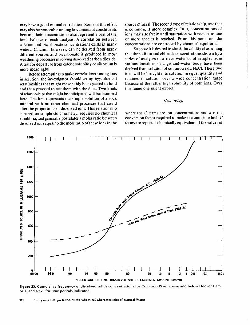
A useful generalization about an array of data, such as a series of chemical analyses of a stream, often may be obtained by grouping them by frequency of occurrence. Figure 23 is a duration diagram showing the dissolved- solids concentration of water in the Colorado River at Grand Canyon, Ariz., from 1926 to 1955 (essentially uncontrolled at that time) compared with the dissolved solids in the outflow at Hoover Dam, the next downstream sampling point from 1937 to 1955. Although the periods of record do not completely coincide, the curves show that the water is much less variable in composition as a result of storage in Lake Mead above Hoover Dam. The median point (represented by 50 percent on the abscissa) for dissolved solids is also higher for the water at Grand Canyon than for virtually the same water after storage,

mixing, and release at Hoover Dam. Daily conductivity values for a period of record may be summarized conveniently by a graph of this type. Figure 24 shows this kind of information for the Ohio River and its two source streams, the Allegheny and Monongahela Rivers in the vicinity of Pittsburgh, Pa. Figures 23 and 24 are time distributions.

A frequency distribution for percent sodium in ground waters from wells in the San Simon artesian basin of Arizona is shown in figure 25. The clustering pattern shown by these data indicates that the waters were of two types, which were identified as occurring in separate areas of the basin. This distribution is not related to time. Other applications of frequency distributions obviously are possible. This type of graphic presentation may be considered most useful as a means of summarizing a volume of data and often gives more information than a simple mean or median value alone would give.

Solute Correlations

The examination of an array of water analyses frequently involves a search for relationships among constituents. Determining the existence of correlations that are sufficiently well defined to be of possible hydrologic or geochemical significance has sometimes been attempted in a random fashion, for example, by preparing many scatter diagrams with concentrations of one component as abscissa and another as ordinate. Commonly, one or more of the diagrams give a pattern of points to which a regression line can be fitted. The statistical procedures for fitting the line, and the evaluation of goodness of fit by a correlation coefficient, provide a means of determining the apparent correlation rather closely in a numerical way. The significance of the correlation in a broader sense, for example, as the indicator of a particular geochemical relationship, is, however, likely to be a very different matter.

Random correlation procedures of the type suggested above are too laborious to do by hand if many analyses are used, but the electronic computer has made this type of correlation a simple process. Accordingly, a wide variety of calculations of this kind could be made, and their significance evaluated later should this procedure offer any reasonable promise of improving the investigator’s understanding of hydrochemical systems.

The difficulties of interpreting random correlations are substantial. The chemical analyses of a series of more or less related samples of water have certain internal constraints that may result in correlations that have slight hydrologic or geochemical significance. For example, the total concentration of cations in milliequivalents per liter in each analysis must equal the total concentration of anions expressed in the same units. If many of the waters in the group being studied have one predominant anion and one predominant cation, these two constituents


may have a good mutual correlation. Some of this effect may also be noticeable among less abundant constituents because their concentrations also represent a part of the ionic balance of each analysis. A correlation between calcium and bicarbonate concentrations exists in many waters. Calcium, however, can be derived from many different sources and bicarbonate is produced in most weathering processes involving dissolved carbon dioxide. A test for departure from calcite solubility equilibrium is more meaningful.

Before attempting to make correlations among ions in solution, the investigator should set up hypothetical relationships that might reasonably be expected to hold and then proceed to test them with the data. Two kinds of relationships that might be anticipated will be described here. The first represents the simple solution of a rock mineral with no other chemical processes that could alter the proportions of dissolved ions. This relationship is based on simple stoichiometry, requires no chemical equilibria, and generally postulates a molar ratio between dissolved ions equal to the mole ratio of these ions in the

source mineral. The second type of relationship, one that is common, is more complex. In it, concentrations of ions may rise freely until saturation with respect to one or more species is reached. From this point on, the concentrations are controlled by chemical equilibria.

Suppose it is desired to check the validity of assuming that the sodium and chloride concentrations shown by a series of analyses of a river water or of samples from various locations in a ground-water body have been derived from solution of common salt, NaCl. These two ions will be brought into solution in equal quantity and retained in solution over a wide concentration range because of the rather high solubility of both ions. Over this range one might expect

CNa=nCCl,

where the C terms are ion concentrations and n is the conversion factor required to make the units in which C terms are reported chemically equivalent. If the values of

16oc

200

Ls III I I I I I 1 lllll 1 I I I II III

999 99 95 90 80 50 20 10 5 2 1 0.5 0.1 0.01

PERCENTAGE OF TIME OlSSOlVEO SOLIDS EXCEEDED AMOUNT SHOWN

Figure 23. Cumulative frequency of dissolved solids concentrations for Colorado River above and below Hoover Dam,

Ariz. and Nev., for time periods indicated.


C are in milliequivalents per liter, n=l. If data are in milligrams per liter, n is the ratio of the combining weight of sodium to the combining weight of chloride, or 0.65.

If the data fit the assumption, a plot of the concentration ofsodium versus the concentration of chloride should give a straight line of slope 1.0 or 0.65, depending on units used. Curvature of the line or deviation from the two permissible slopes indicates that the hypothesis is incorrect. If one plots log CNa versus log Ccl, a straight line also should be obtained, but it will have a slope of 1.0 and an intercept of log n.

Figure 26 is a plot of sodium concentrations versus chloride concentrations, in meq/L, for samples from the Gila River at Bylas, Ariz. The curved part of the regression line shows that sources of the ions other than common salt are involved, although at the higher concentrations the theoretical slope of 1.0 is closely approached.

The correlation cited above does not involve much chemistry and is too simplified to have much practical value. If considerations of solubility are involved, the constituents may be correlated in a different way. For example, the solution of calcium and sulfate can continue

only up to the solubility limit of gypsum. When this level is reached, at equilibrium the solubility-product relationship would hold. The two conditions would be (1) for dilute solutions,

c ca2+=rzc~042-,

and (2) at saturation,

[Ca”‘] [S042+]=KSp,

where KS,) is the solubility product.

Figure25. Number of water samples having percent-sodium

values within ranges indicated, San Simon artesian basin,

Arizona.

1400 II II I I I I I I I I I I I I I II III II)

2 I3OO- A 8 2 IZOO-

p3 g IIOO-

z z lwo-

E

k E z 800- ”

E 700 -

3

i soo-

& g wo- f

& f 400 -

c 3 4 300-

8 0 200- E G 5 IOO-

-

Ensmple The SDICI~IC conductrncr of thr Yonon- Eahala lhvn al Charlrrol mar br r~poctod to rrcred 200 mlcromhos for SO porcrd

0' III II I I I I I I I I I I I I II III 001 0050102 05 I 2 5 10 20 30 40 so 60 70 80 so 95 98 99 99.5 99 8 99.9 99.99

PERCENTAGE OF TIME THAT SPECIFIC C~~~~~CTANCE EQUALED oft EXCEEDED THAT SHOWN

Figure 24. Cumulative frequency of conductance, Allegheny, Monongahela, and Ohio River waters, Pittsburgh area,

Pennsylvania, 1944-50.


If the influence of ionic strength and ion-pair formation are ignored for the moment, one could represent the second equation in terms of concentrations rather than activities so that the same variables would be present in both expressions. All concentrations are expressed in moles per liter.

The first equation would give a straight line if calcium concentrations were plotted against sulfate. The second equation, however, is for a hyperbola, and therefore an attempt to make a linear correlation of a group of analyses, including concentrations affected by both relationships, is likely to give ambiguous results. If both expressions are placed in logarithmic form, as follows, however, both give straight lines:

lofit Cc*=lw Go.,

This is a very simple form of a reaction-path simula- tion. A model of this type uses a series of equilibria or stoichiometric processes to exphrin changes in composition observed along the flow path of water in an aquifer or other system of interest. Geochemical models using this approach were described by Plummer and others (1983). A similar progression of controls can be observed during the process of evaporation.

A more complicated equilibrium is that for calcite solubility; it involves three variables, as noted earlier:

[Ca”‘] [HCO;] [H+l -=Ks

This could still be converted to a two-variable relationship by combining the bicarbonate and hydrogen ion into a single term, as follows:

log Cc,=log K’-log C,,.

The first relationship should hold up to the point where precipitation of gypsum begins, and the second, thereafter. A break in slope of the regression line would occur at that point. It should be noted that in this example K’ is a conditional equilibrium constant that includes the effects of ionic strength and ion-pairing. Therefore, the value of K’ increases as concentrations increase, and the nature of the correlation under conditions of saturation is more complex than this treatment implies.

40 I I I 0

[&“+I . [HCo3-1 =K -. W’l ’

[ HCOs-] log [Ca’+]+log --

@I =log K,.

However, a more useful graphical technique for representing this equilibrium by itself is to use a pH overlay on a plot of log [Ca”‘] versus log [IICOa-] as in plate 2. The applicability and potential modifications of this diagram were discussed in the section of this book dealing with calcium chemistry.

The degree to which correlations of the types men- tioned above can be obtained is of geochemical significance in many systems. Analyses may be checked for conformance to equilibrium with several solids at once. For example, one might want to examine data for equilibrium with gypsum and calcite. Figure 27 is one approach to this type of correlation. Several analyses from tables 11 and 15 are plotted in the diagram. This relationship also could be represented as

CaCOa(c)+H’+SOt-=CaS04(c)+HCOB-,

WC%1 [H’l .[S0.,2-]=K,

or F-=03-1

log - W’l

+log fS042-]=10g K,

CHLORIDE, IN MILLIEQUIVALENTS PER LITER

Figure 26. Relationship of chloride to sodium, Cila River at Bylas, Ariz., October 1, 1943, to September 30, 1944.

where K is a combination of the two constants for the solubility equilibria for gypsum and calcite.


There are other combinations of equilibria that than these simple examples. The characteristics of various might be significant in ground-water systems and at low models were summarized by Nordstrom, Plummer, and flow in some streams. For example, the relationship of others (1979). The models can test water analyses for cation-exchange equilibria in soil to the solubility of possible equilibrium with a large number of minerals, calcite could be studied in this way. over a range of temperatures and ionic strengths.

The abscissa and ordinate in figure 27 represent ion-activity products for the calcite-solubility equilibrium and the solubility-product equation for gypsum. Values greater than the equilibrium constant indicate supersaturation with respect to these two solids. The activities of the ions must be calculated from analytical concentrations with due attention to the effects of ionic strength and complex or ion-pair formation. Irrigation drainage water in some areas evolves to a composition that is near saturation with respect to both solids (Hem, 1966).

The statistical technique, factor analysis, has been used by some investigators to develop or refine correlations among solutes and environmental factors. Dawdy and Feth (1967) used this approach to study controls of ground-water composition in the Mojave River valley near Victorville, Calif. The first of a series of four papers (Reeder and others, 1972) on chemistry of water and sediments in the Mackenzie River system in Canada used this technique to aid in the assignment of sources to the solute load of this large northern river.

A study by Feth and others (1964) of water composition associated with granitic rocks uses diagrams on which areas of stability for different rock minerals are shown in terms of activity of silica as abscissa and ratios of sodium or potassium to hydrogen activity as ordinate. These diagrams follow models used by Garrels and Christ (1964, p. 352-378) and have been used widely in evaluating the effects of the weathering of silicate rocks. How- ever, some of the reactions involved in silicate dissolution and clay-mineral synthesis are incongruent, and these stability diagrams, which are based on assumed thermo- dynamic equilibrium, have only a limited usefulness in predicting solute concentrations to be expected in natural systems.

Graphical Methods of Representing Analyses

Over the years, a considerable number of techniques for graphical representation of analyses have been proposed. Some of these are useful principally for display purposes-that is, to illustrate oral or written reports on water quality, to provide means for comparing the analyses with each other, or to emphasize differences and similarities. Graphical procedures do this much more effectively than numbers presented in tables.

The development of computerized chemical models makes it possible to handle systems that are more complex

In addition to the types of graphs suitable for displays and comparison of analyses, graphical procedures have been devised to help detect and identify mixing of waters of different composition and to identify some of the chemical processes that may take place as natural waters circulate. Graphing techniques of the latter type may be useful in the study of data prior to preparing reports or arriving at conclusions. Some of the graphical techniques that appear to be useful are described here, but this discussion is not intended to include all the methods that have been suggested in the literature. Graphing of water analyses is a study technique and not an end in itself.

-2 I I I 8

-3

t

Swersaturatlon Gypsum

4

-6 Unsaturated

I I

Supersaturation Gypsum and Calate 1

,114

Supersatur8tlon CalcIte -I

Log ICal+log [HCO~l+PH

Figure 27. Calcite and gypsum equilibrium solubility rela-

tionships, 25OC and 1 atmosphere pressure. Plotted points

represent analytical data from tables 11 and 15 (e.g., “ll- l”=table 11, analysis 1).

Ion-Concentration Diagrams

Most methods of graphing analyses are designed to represent simultaneously the total solute concentration and the proportions assigned to each ionic species for one analysis or a group of analyses. The units in which concentrations are expressed in these diagrams generally are milliequivalents per liter.

In the ion-concentration graphing procedure origin- ated by the late W. D. Collins (1923), each analysis is represented by a vertical bar graph whose total height is proportional to the concentration of determined anions or cations, in milliequivalents per liter. The bar is divided by a vertical line, with the left half representing cations and the right half anions. These segments are then divided by horizontal lines to show the concentrations of the


major ions, and these ions are identified by distinctive colors or patterns. Usually six divisions are used, but more can be used if necessary. The concentrations of closely related ions are often added together and represented by a single pattern.

An example of Collins’ ion-concentration graphing procedure representing four analyses from tables in this book is given in figure 28. (The other graphing procedures discussed here are for the most part illustrated with the same four analyses.) The Collins’ system as described does not consider nonionic constituents, but they may be represented, if desired, by adding an extra bar or other indicating device with a supplementary scale. In figure 29, the hardness of two waters is shown. The hardness in milligrams per liter as CaCOa is equivalent to the height of the calcium plus the magnesium segments, in milliequivalents per liter, multiplied by 50. In figure 30, the concentration of silica is represented in millimoles per liter, because milliequivalents cannot be used for un- charged solute species or species whose form in solution

30 EXPLANATION

29

Na+K CI+NO

28

27

Figure 28. Analyses represented by bar lengths in milli- Figure 30. Analyses represented by bar lengths in milliequivalents per liter. Numbers above bars indicate source equivalents per liter, with dissolved silica in millimoles per of data in tables 10, 12, 15, and 17 (e.g., “12-6”=table 12, liter. Numbers above bars indicate source of data in tables analysis 6). 12, 15, and 17 (e.g., “12-6”=table 12, analysis 6).

Figure 29. Analyses represented by bar lengths in milli-

equivalents per liter, with hardness values in milligrams per

liter. Numbers above bars indicate source of data in tables

12 and 15 (e.g., “12-6”=table 12, analysis 6).

EXPLANATION


is not specifically known. The units are closely related to milliequivalents per liter, and this type of graph will be used in depicting analyses of water associated with different rock types later in this book. The pattern representing silica occupies the full width of the bar graph because the solute species H&04 consists of a silicate anion whose charge is balanced by H’. This modification is sometimes useful in showing results of geochemical processes. The concentration of silica in millimoles per liter is readily computed from gravimetric data in water- analysis tabulations.

A system of plotting analyses by radiating vectors proposed by Maucha (1949) of Hungary is illustrated in figure 31. The distance each of the six vectors extends from the center represents the concentration of one or more ions in milliequivalents per liter. This plotting system has not been used widely, but it may have some potential as a means of showing analytical values in a small space, for example, as a symbol on a map. A system suggested by Stiff (1951) seems to give a more distinctive pattern and has been used in many papers, especially those dealing with oilfield waters. The Stiff plotting technique uses four parallel horizontal axes ex- tending on each side of a vertical zero axis. Concentrations of four cations can be plotted, one on each axis to the left of zero, and likewise four anions concentrations can be plotted, one on each axis to the right of zero; the ions should always be plotted in the same sequence. The concentrations are in milliequivalents per liter. The resulting points are connected to give an irregular polygonal shape or pattern, as in figure 32. The Stiff patterns can be

No + K

0 5 10 I ., 1

MllLlEOUlVAtENTS PER LITER

Figure 31. Analyses represented by vectors based on milli-

equivalents per liter. Numbers near symbols indicate source

of data in tables 10, 12, 15, and 17 (e.g., “12-6”=table 12,

analysis 6).

a relatively distinctive method of showing water-composition differences and similarities. The width of the pattern is an approximate indication of total ionic content. Stiff patterns were used as map symbols by Halberg and others (1968).

Two other procedures that have been used to prepare pattern diagrams are worthy of mention. The “pie” diagram can be drawn with a scale for the radii which makes the area of the circle represent the total ionic concentration (fig. 33) and subdivisions of the area represent proportions of the different ions. Colby and others (1956) used a pattern diagram in which four components, Ca+Mg, C03+HCOa, Na+K, and Cl+S04+N03, were represented on rectangular coordinates. The kitelike figure resulting from connecting the four points made a con- venient map symbol (fig. 34).

A nomograph proposed by Schoeller (1935) and modified by R. C. Vorhis of the U.S. Geological Survey is shown in figure 35. This diagram is a means of depicting

I I I I I I I I 1 30 25 20 15 10 5 0 5 10 15 20

CATIONS, IN MlLLlEOUlVALENTS ANIONS. IN MILLIEOUIVALENTS PER LITER PEA LITER

Figure32. Analyses represented by patterns based on milli-

equivalents per liter. Numbers near patterns indicate source

of data in tables 10, 12, 15, and 17 (e.g., “12-6”=table 12,

analysis 6).


a group of analyses that has the advantage of also showing relationships among milligrams per liter and milliequivalents per liter for the different ions. Waters of similar composition plot as near-parallel lines. This diagram, however, uses logarithmic scales, and this may complicate the interpretation for waters that differ greatly in concentration,

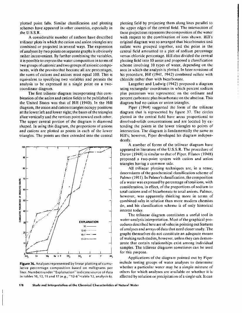
Figure 36 is a cumulative percentage plot of analyses in milligrams per liter. This method of graphing permits differentiating between types of water on the basis of the shape of the profile formed by joining the successive points.

Some other graphical display techniques used in study of oil-field brines were described by Collins (1975, p. 128-132).

Ion-concentration diagrams are useful for several purposes. They aid in correlating and studying analyses and are especially helpful to the novice in this field. They also aid in presenting summaries and conclusions about water quality in areal-evaluation reports. The Collins’ diagram can serve as an effective visual aid in oral

presentations on water compos;ition for semitechnical and nontechnical groups. For this purpose, the bar symbols can be made at a scale of about 10 cm = 1 meq/L, by using cards fastened together end to end with hinges of flexible tape to give a length sufficient to represent the total concentration of ions. Segments representing the ions are then drawn on the graph, and they can be colored distinctively to show the six species. While discussing the analyses, the lecturer can take out the appropriate set of cards and hang them up in view of the audience. The contrast between water of low concentration shown by only one or two cards and more concen- trated solutions, occurring naturally or as a result of pollution, shown perhaps by a thick stack of cards that might reach a length of 20 ft when unfolded, is a potent attention-getter.

Trilinear Plotting Systems

If one considers only the major dissolved ionic constituents in milliequivalents per liter and lumps potassium and sodium together and iluoride and nitrate with

Na +K

0 1 5 10 50 100 I I I

SCALE OF RADII t TOTAL OF MlLLlEClUlVALENTS PER LITER I

Figure 33. Analyses represented by circles subdivided on the basis of percentage of total milliequivalents per liter. Numbers

above circles indicate source of data in tables IO, 12, 15, and 17 (e.g., “12-6”=table 12, analysis 6).


chloride, the composition of most natural waters can be closely approximated in terms of three cationic and three anionic species. If the values are expressed as percentages of the total milliequivalents per liter of cations, and of anions, the composition of the water can be represented conveniently by a trilinear plotting technique.

The simplest trilinear plots use two equilateral triangles, one for anions and one for cations. Each vertex represents 100 percent of a particular ion or group of ions. The composition of the water with respect to cations is indicated by a point plotted in the cation triangle, and the composition with respect to anions by a point plotted in the anion triangle. The coordinates at each point add to 100 percent.

Emmons and Harrington (1913) used trilinear plots in studies of mine-water composition. This application was the earliest found by the writer in surveying published literature on water composition, even though Emmons and Harrington do not claim originality for the idea of using trilinear plots for this purpose. In the form used by Emmons and Harrington, the cation triangle lumps calcium with magnesium at one vertex and sodium with potassium at another. This leaves the third vertex for “other metals” that might be present in the mine waters that were of principal interest to these investigators. For most natural water, the concentration of these other metals is not a significant percentage of the total.

Dela 0. Carefio (1951, p. 87-88) described a method of trilinear plotting, which he attributed to Hermion Larios, that combines the plotting with a classification and reference system. The three principal cations are plotted conventionally in one triangle and the three

0 5 IO 15 20 25 30 I,,~,I~~,,Il~llI,,~,I~,~~I~~~II

MltLlLOUlVALENTS PER LITER

CO- S0,+Cl+N03/

Figure34. Analyses represented by patterns based on com- Figure 35. Analyses represented by logarithmic plotting of bined anion and cation concentrations. Numbers above concentration in milligrams per liter. Numbers under “Ex- patterns indicate source of data in tables 10,12,15, and 17 planation” indicate source of data in tables IO, 12,15, and

(e.g., “12-6”=table 12, analysis 6). 17 (e.g., “12-6”=table 12, analysis 6).

anions in another. Each triangle is divided into 10 approximately equal areas numbered from zero to nine. A two-digit number is then used to characterize the water. The first digit is the number of the area within the cation triangle in which the water plots. The second digit is the number of the area in the anion triangle in which the

LOGARITHMIC NOYOCRAPH N, FOR

WATER-ANALYSIS DATA

ALL NMSTITUENTS IN ml/l

EXPLANATION 10,----I=


plotted point falls. Similar classification and plotting schemes have appeared in other countries, especially in the U.S.S.R.

A considerable number of authors have described trilinear plots in which the cation and anion triangles are combined or projected in several ways. The expression ofanalyses by two points on separate graphs is obviously rather inconvenient. By further combining the variables, it is possible to express the water composition in terms of two groups of cationic and two groups of anionic components, with the proviso that because all are percentages, the sums of cations and anions must equal 100. This is equivalent to specifying two variables and permits the analysis to be expressed as a single point on a two- coordinate diagram.

The first trilinear diagram incorporating this combination of the anion and cation fields to be published in the United States was that of Hill (1940). In the Hill diagram, the anion and cation triangles occupy positions at the lower left and lower right; the bases of the triangles aline vertically and the vertices point toward each other. The upper central portion of the diagram is diamond shaped. In using this diagram, the proportions of anions and cations are plotted as points in each of the lower triangles. The points are then extended into the central

90 -

EXPLANATION

10 -

12-e.. . . . .

15-1 -. -

17-3---

Na + K CO3 Cl F No3

Figure 36. Analyses represented by linear plotting of cumu-

lative percentage composition based on milligrams per

liter. Numbers under “Explanation”indicate source of data

in tables 10,12,15 and 17 (e.g., “12-6”=table 12, analysis 6).

plotting field by projecting them along lines parallel to the upper edges of the central field. The intersection of these projections represents the composition of the water with respect to the combination of ions shown. Hill’s original diagram was so arranged that bicarbonates and sulfate were grouped together, and the point in the central field amounted to a plot of sodium percentage versus chloride percentage. Hill also divided the central plotting field into 10 areas and proposed a classification scheme involving 10 types of water, depending on the area in which the analysis is plotted. In later revisions of his procedure, Hill (1941, 1942) combined sulfate with chloride rather than with bicarbonate.

Langelier and Ludwig (1942) proposed a diagram using rectangular coordinates in which percent sodium plus potassium was represented on the ordinate and percent carbonate plus bicarbonate on the abscissa. This diagram had no cation or anion triangles.

Piper (1944) suggested the form of the trilinear diagram that is represented by figure 37. The circles plotted in the central field have areas proportional to dissolved-solids concentrations and are located by ex- tending the points in the lower triangles to points of intersection. The diagram is fundamentally the same as Hill’s; however, Piper developed his diagram indepen- dently.

A number of forms of the trilinear diagram have appeared in literature of the U.S.S.R. The procedure of Durov (1948) is similar to that of Piper. Filatov (1948) proposed a two-point system with cation and anion triangles having a common side.

All trilinear plotting techniques are, in a sense, descendants of the geochemical classification scheme of Palmer (1911). In Palmer’s classification, the composition of a water was expressed by percentage of total ions, with consideration, in effect, of the proportions of sodium to total cations and of bicarbonate to total anions. Palmer, however, was apparently thinking more in terms of combined salts in solution than more modern chemists do, and his classification scheme is of only historical interest today.

The trilinear diagram constitutes a useful tool in water-analysis interpretation. Most of the graphical procedures described here are of value in pointing out features of analyses and arrays of data that need closer study. The graphs themselves do not constitute an adequate means of making such studies, however, unless they can demon- strate that certain relationships exist among individual samples. The trilinear diagrams sometimes can be used for this purpose.

Applications of the diagram pointed out by Piper include testing groups of water analyses to determine whether a particular water may be a simple mixture of others for which analyses are available or whether it is affected by solution or precipitation of a single salt. It can


be shown easily that the analysis of any mixture of waters A and B will plot on the straight line AB in the plotting field (where points A and B are for the analyses of the two components) if the ions do not react chemically as a result of mixing. Or, if solutions A and C define a straight line pointing toward the NaCl vertex, the more concen- trated solution represents the more dilute one spiked by addition of sodium chloride.

Plotting of analyses of samples from wells succes- sively downslope from each other may show linear trends and other relationships that can be interpreted geochem- ically. Poland and others (1959) used trilinear diagrams

DISSOLVED SOLIDS

0 12-6

extensively in studying contamination of ground water by seawater and other brines along the California coast near Los Angeles. The relationships shown by the diagrams usually constitute supporting evidence for conclusions regarding water sources that also have other bases of support.

Trilinear diagrams continue to be used in papers dealing with natural-water chemistry and geochemistry. A few examples are cited here to indicate the varieties of applications. Maderak (1966) used trilinear diagrams to show trends in composition as streamflow volume changed at several sampling points on the Heart River in

, $2-6

CATIONS PERCENT OF TOTAL MILLIEQUIVALENTS PER LITER

ANIONS

Figure 37. Trilinear diagram showing analyses represented by three-point plotting method. Numbers near circles indicate

source of data in tables 10, 12, 15, and 17 (e.g., “12-6”=table 12, analysis 6).


western North Dakota. Hendrickson and Krieger (1964) and Feth and others (1964) used the diagram as a means of generally indicating similarities and differences in the composition of water from certain geologic and hydrologic units. Bradford and Iwatsubo (1978) used the diagrams to show effects of logging and other factors on stream-water composition in the area of Redwood Na- tional Park, Calif. Trilinear diagrams were used by White and others (1980) to help correlate rock and water composition in the ground water of Ranier Mesa, Nev. Many other papers could be cited. The trilinear diagram has been widely used by U.S. Geological Survey hydrologists.

A compilation of methods for graphical representation of water analyses that had been described in the literature up to that time, was prepared by Zaporozec (1972).

Methods of Extrapolating Chemical Data

A considerable part of the task of interpreting water- quality data can be extrapolating or interpolating. For example, a few analyses of river-water samples taken at irregular intervals may need to be used to estimate a continuous record, or analytical records may need to be extended backward or forward in time by correlating the analyses with some other measured variable. For ground- water studies, variations in time generally are less important than variations from place to place in the composition of a ground-water body, and procedures are needed for extrapolating analyses representing individual wells or springs to cover the whole volume of ground water of an area.

The extension of individual observations of river- water composition can be accomplished by several averaging techniques or other statistical treatments already discussed. As the technology of on site observations of water quality has matured, more complete chemical records are being computed from continuously measured specific conductance. This sort of calculation can provide fairly dependable values for major ions, at least for many streams. The accuracy of the calculated value depends on how good a correlation of the measured with the calculated properties can be established from previous records of a more complete nature.

Water-Quality Hydrographs

A graph showing the changes over a period of time of some property of water in a stream, lake, or underground reservoir is commonly termed a “hydrograph.” Hydrographs showing variability of a property of river water with time are often used as illustrations in reports. An example is figure 4, which shows the change with time of the conductivity of water in the Rio Grande at

San Acacia, N.M. For a stream, where changes with time can be large and can occur rapidly, an accurate extrapolation cannot be made on the basis of time alone. On that basis, it is possible to state only approximately what the composition of water would be at different times of the year. In contrast, streams that are controlled by storage reservoirs (the Colorado River bselow Hoover Dam, for example), streams that derive most or all of their flow from ground-water sources (the Niobrara River, for example, which drains the sandhill region of northwestern Nebraska), and streams that have very large discharge rates (the Mississippi River at New Orleans, for example) may exhibit only minor changes in composition from day to day or even from year to year.

Streams whose flow patterns have been altered extensively by humans may show definite long-term trends as the water quality adjusts to the new regime. The Gila River at Gillespie Dam, Ariz., for example, showed a deteriorating quality over many years of record as irrigation depleted the upstream water supply (Hem, 1966).

In ground water, the changes in quality with time are normally slow. The illustrations already given in this paper, however, show that both long-term and short- term trends can be observed. The slow increase in dissolved solids that occurred in the ground water of the Wellton-Mohawk area of Arizona (fig. 7) represents a condition related to water use and development, but shorter term fluctuations may be related to well construction and operation (fig. 5) or to changing recharge rates, evapotranspiration, or other factors that often influence water near the water table observed in shallow wells or seasonal springs (fig. 6). Deep wells that obtain water from large ground-water bodies that are not too extensively exploited and many thermal springs may yield water of constant composition for many years. Analyses published by George and others (1920) for Poncha Springs near Salida, Colo., represented samples collected in 1911. A sample of a spring in this same group collected in 1958 (White and others, 1963) gave an analysis that did not differ by more than ordinary analytical error from the one made 47 years before, with the exception of the sodium and potassium. The potassium values reported by George and others (1920) appear too high and sodium too low, in comparison with the modern analysis, but the total of the two alkali metals is nearly identical in both analyses.

Water Quality in Relation to Stream Discharge

The concentration of dissolved solids in the water of a stream is related to many factors, but it seems obvious that one of the more direct and important factors is the variable volume of liquid water from rainfall available for dilution and transport of weathering prod-


ucts. Presumably, therefore, the dissolved-solids concentration should be an inverse function of the rate of discharge of water over all or at least most of the recorded range. In discussing averaging of river-water chemical analyses, some of the complications that influence discharge versus dissolved-solids concentration relationships have been pointed out. There will no doubt, however, be a continuing demand to know how well the composition of a river water can be computed from the water- discharge rate and some previous record of composition. Some further consideration of the subject, therefore, is needed. The goal would be to obtain a dissolved-solids rating curve for a stream-measuring station: a graph of dissolved-solids concentration versus water-discharge rate, expressing their correlation.

The development of such a correlation requires a preliminary assessment that might be termed a “concep- tual model.” The model can then be tested for validity and to determine what kinds of information might be required to develop it completely. A consistent relationship between water discharge and total solute concentration ought to be observed in a stream that receives a large part of its mineral load from a rather constant saline inflow upstream from the measuring point and whose runoff from other sources is constant and low in dissolved-solids concentration. A finite relationship can be expected to hold for any single unreactive dissolved component. No stream meets these specifications completely, and few streams that might approach them have been studied closely.

The simplest dilution model for a particular solute in a reach of river assumes, then, that a constant total load of solute is entering upstream and that the observed concentration of that solute at the sampling point varies owing to dilution by runoff. If other factors are insignifi- cant, this condition can be evaluated from a simplified solute-balance equation:

where

Ci=concentration of solute before dilution, Q1=volume of flow before dilution, Cz=concentration of solute in diluting water, and Q2=volume of dilution water, C3=final concentration observed.

The three terms in this equation represent loads of solute, and an inflow-outflow balance is assumed (that is, it is assumed there is no change in storage).

If the concentration of solute in the diluting water is zero, then CzQ2 drops out and

CiQi is constant and can also be represented as WI, the total original solute load. This is the equation of a hyperbola. If expressed in logarithmic form, however,

log G=log WI-log (&I+ Qz),

it has the form of a straight line, with slope -1.0. Thus, the degree to which a particular set of concentration and stream-discharge data fits the simple dilution model can be tested by plotting these variables on log-log paper.

Of course, most natural systems can display a simple dilution mechanism only over a limited range of concentration. Normally, the dilution water contains some of the same solute as the water being diluted, and this will cause the high-discharge end of the plot to approach a minimum near the concentration present in the diluting water. At the low-discharge end, Qa approaches zero and the value of Cs will become equal to the concentration of solute in the inflow source. The solubility of the ion being considered, or other factors independent of discharge, also may limit the ion’s concentration at low discharge, so the slope of the curve will tend to flatten at very low discharge. It is obvious that complexities in most natural systems tend to make the equation considerably more complicated. For example, if some of the solute being considered is present in the runoff, the value of CZ will not be zero, and the final equation will have the form

If expressed in logarithmic terms, this equation would give a curved line, as C2Q2 is unlikely to be constant and probably will vary in response to discharge.

A practical difficulty inherent in the use of the log-log type of plot is that observed solute concentrations commonly show a rather narrow range of variation, and considerable clustering of points may occur. It is of interest, however, to use this approach to explore the relationships between discharge and solute concentration obtainable from existing records.

In past years, in studies by the U.S. Geological Survey, the only chemical determination made for each daily sample usually was specific conductance, and many of these data have never been published. Discharge information readily available for use with these determinations is the published daily mean rate of flow. An instantaneous sample may not be a good representation of the daily mean conductivity, and some values thus may be poorly


suited for establishing a meaningful discharge-conductivity relationship. However, if a well-defined relationship exists, it will not be completely obscured, although individual points may be scattered. Records collected for the specific purpose of exploring water-quality-water-discharge relationships must be obtained carefully with the aim of getting fully compatible data for both variables. This is perhaps most effectively accomplished by simulta- neous continuous measurement of water-discharge rate and solute concentration.

A sampling station whose characteristics might be suitable for establishing a dissolved-solids versus discharge relationship was operated for a time by the U.S. Geologi- cal Survey on the San Francisco River at Clifton, in southeastern Arizona. About 60 percent of the annual dissolved-solids load of the river there was contributed by saline inflow from the Clifton Hot Springs, a short distance above the gaging station and about 1% miles above the sampling section. The varying amounts of discharge from the direct runoff and a more constant amount of dilute base flow of the river above the springs might be considered dilution factors controlling the concentration observed at the sampling point.

I---

Y

Specific conductance of water at this station should approach a high limiting value near the conductance of the spring inflow (about 16,000 pmho/cm) at low discharge, and a minimum value fi lted by the conductance of runoff, which has had only a brief opportunity to react with near-surface rock and soil minerals, at high discharge. The lower limiting value can be (estimated only approximately from the sampling record, but it is probably about 200 pmho.

Figure 38 is a logarithmic plot of specific conductance of daily samples versus daily mean discharge for the 1944 water year for the San Francisco River at Clifton, Ariz. Some daily values were omitted where the points are closely grouped. The scatter of points is substantial, and it would be difficult to fit them to a straight line. Furthermore, the slope of such a line is not -1.0. Both facts suggest that the simple dilution equation derived in the earlier discussion is not directly applicable.

From other information about the quality of water at this point, however, it is possible to derive a more pertinent relationship. The solute load at the sampling point may be considered to have three components, represented by C,Q,, terms, in which C represents con-

I I I Illlll I I I Illlll I I llllr

I I lllll I I lllll I I lI1lI 50 100 500 1000

DAILY MEAN DISCHARGE, IN CUBIC FEET PER SECON’D

5000

Figure 38. Specific conductance of daily samples and daily mean discharge, San Francisco River ar Clifton, Ark., October 1,

1943, to September 30,1944. Circles represent observed values. Symbols “x” are calculated values based on postulated

relationship in text.


ductance in micromhos and Q represents discharge of water in cubic feet per second (cfs). CIQl represents the solute load brought in by spring inflow. This water has a specific conductance of about 16,000 pmho, and the flow is considered constant at 2 cfs (Hem, 1950). CZ@ represents base solute load of the river above the springs that dilutes the spring inflow. For simplicity, this water is assumed from available analyses of samples taken above the inflow zone to have a specific conductance of 500 pmho and a maximum flow rate of 100 cfs. CaQ3 represents flood runoff, constituting all flow above 102 cfs, and is assigned a specific conductance of 200 pmho. The mixture of all these is represented by concentration CF. The equation for predicting concentration at this station from water-discharge data becomes

Substituting appropriate values from quantities postulated above gives the points with the symbol “x” in figure 38. The dashed curve fitted to these points smooths out some of the irregularities that would result if more calculated points were used, but demonstrates an approximate fit of the model to actually observed conditions.

The scatter of observed points is substantial; therefore, there would be substantial uncertainty in conductance values calculated from discharge by means of any curve fitted to the points. Some of the spread in points in figure 38 may have resulted from changes in rate of spring inflow, and some might have been caused by incomplete mixing of the inflow with the river water at the sampling point. Most of the scatter, however, is probably related to the failure of individual samples to represent the average composition of the river for a whole day.

The San Francisco River is subject to rapid changes in stage, especially during the summer when heavy local thunderstorms often occur in the afternoon and early evening. The resulting runoff events commonly occur at night, and the river stage was frequently near the low point for the day when samples were collected. Sampling was always done during the daytime, and the probability of a sample’s representing the day’s average composition was not always good during the summer storm period.

Another approach to the construction of discharge- concentration models has been to develop a mathematical relationship that best fits a set of observed points. For example, Steele (1968a, b) studied the relationships of dissolved-ion concentration to water discharge of Pes- cadero Creek, a small northern California coastal stream, and reported that his data fitted the relation CQ=K, or log C=log K-Nlog Q. The exponent N can be evaluated from the slope of the regression line. This exponent does not, however, represent a simple hydrologic parameter.

It is empirical and represents several kinds of hydrologic effects.

Other investigators who have developed dissolved- solids rating curves include Durum (1953), who found a reasonably good correlation between chloride concentration and discharge for the Saline River near Russell, Kans., and Hendrickson and Krieger (1964), who found reasonably consistent relationships between specific conductance and discharge for the Salt River at Shepherds- ville, Ky., for low-flow periods.

In streams for which runoff patterns and solute- load sources are more complicated, a poorly defined relationship between discharge and dissolved-solids concentration is to be expected. An interesting feature observed in many streams, although closely studied in only a few places, is a tendency for the water of a rising stage to have a considerably higher dissolved-solids concentration than the water passing the sampling point at an equal flow rate after the peak discharge has passed. Hendrickson and Krieger (1964 p. 123) presented a semilog graph of conductance (on the x-axis) versus log of discharge which shows a counterclockwise loop that ideally would be characteristic of observations during a flood event. At first the conductance is nearly constant as discharge rises; then the conductance begins to decrease as the peak stage is reached, continues to decrease after the flow begins to recede, and, finally, increases with falling stage until the starting point on the graph is again reached. Flood observations showing several looping cycles were presented by these investigators for the Salt River at Shepherdsville, Ky.

Toler (1965) observed a clockwise loop in his study of the relation of dissolved solids to discharge for Spring Creek in southwestern Georgia. The effect was attributed to an increasing contribution from ground water during falling stages that resulted from the rapid circulation of water through the limestone of the drainage basin.

The factors that control the concentration of water early in a flood event obviously are different for different streams and sampling points. In general, however, when a sudden large inflow of water occurs upstream from a sampling point, the flood wave moving down the channel tends to push water already in the channel ahead of it. If the stream had a low or moderate flow rate before the rise began, the water in the channel would be relatively high in dissolved-solids concentration, and as the wave moved downstream a large volume of this more highly mineralized water might accumulate in the wave front.

The effect of water-discharge rate on water composition may obscure the effect of other factors one might wish to evaluate. The analysis of long-term records to evaluate water-quality trends can be accomplished by establishing a correlation between discharge and solute concentration and then looking for systematic departures from the relationship. Some procedures for detecting


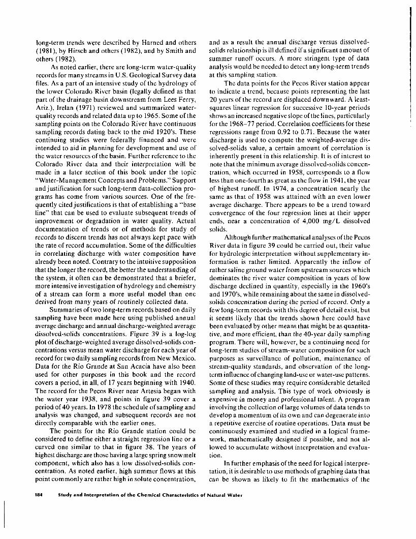
long-term trends were described by Harned and others (1981) by Hirsch and others (1982), and by Smith and others (1982).

As noted earlier, there are long-term water-quality records for many streams in U.S. Geological Survey data files. As a part of an intensive study of the hydrology of the lower Colorado River basin (legally defined as that part of the drainage basin downstream from Lees Ferry, Ariz.), Irelan (1971) reviewed and summarized water- quality records and related data up to 1965. Some of the sampling points on the Colorado River have continuous sampling records dating back to the mid 1920’s. These continuing studies were federally financed and were intended to aid in planning for development and use of the water resources of the basin. Further reference to the Colorado River data and their interpretation will be made in a later section of this book under the topic “Water-Management Concepts and Problems.” Support and justification for such long-term data-collection programs has come from various sources. One of the frequently cited justifications is that of establishing a “base line” that can be used to evaluate subsequent trends of improvement or degradation in water quality. Actual documentation of trends or of methods for study of records to discern trends has not always kept pace with the rate of record accumulation. Some of the difficulties in correlating discharge with water composition have already been noted. Contrary to the intuitive supposition that the longer the record, the better the understanding of the system, it often can be demonstrated that a briefer, more intensive investigation of hydrology and chemistry of a stream can form a more useful model than one derived from many years of routinely collected data.

Summaries of two long-term records based on daily sampling have been made here using published annual average discharge and annual discharge-weighted average dissolved-solids concentrations. Figure 39 is a log-log plot of discharge-weighted average dissolved-solids concentrations versus mean water discharge for each year of record for two daily sampling records from New Mexico. Data for the Rio Grande at San Acacia have also been used for other purposes in this book and the record covers a period, in all, of 17 years beginning with 1940. The record for the Pecos River near Artesia began with the water year 1938, and points in figure 39 cover a period of 40 years. In 1978 the schedule of sampling and analysis was changed, and subsequent records are not directly comparable with the earlier ones.

The points for the Rio Grande station could be considered to define either a straight regression line or a curved one similar to that in figure 38. The years of highest discharge are those having a large spring snowmelt component, which also has a low dissolved-solids concentration. As noted earlier, high summer flows at this point commonly are rather high in solute concentration,

and as a result the annual disclnarge versus dissolved- solids relationship is ill defined ifa significant amount of summer runoff occurs. A more stringent type of data analysis would be needed to detect any long-term trends at this sampling station.

The data points for the Pecos River station appear to indicate a trend, because points representing the last 20 years of the record are displaced downward. A least- squares linear regression for successive lo-year periods shows an increased negative slope of the lines, particularly for the 1968-77 period. Correlation coefficients for these regressions range from 0.92 to 0.71. Because the water discharge is used to compute the weighted-average dissolved-solids value, a certain amount of correlation is inherently present in this relationship. It is of interest to note that the minimum average dissolved-solids concentration, which occurred in 1958, corresponds to a flow less than one-fourth as great as the flow in 1941, the year of highest runoff. In 1974, a concentration nearly the same as that of 1958 was attained with an even lower average discharge. There appears to be a trend toward convergence of the four regression lines at their upper ends, near a concentration of 4,000 mg/L dissolved solids.

Although further mathematical analyses of the Pecos River data in figure 39 could be carried out, their value for hydrologic interpretation without supplementary information is rather limited. Apparently the inflow of rather saline ground water from upstream sources which dominates the river water composition in years of low discharge declined in quantity, especially in the 1960’s and 1970’s, while remaining about the same in dissolved- solids concentration during the period of record. Only a few long-term records with this degree of detail exist, but it seems likely that the trends shown here could have been evaluated by other means that might be as quantitative, and more efficient, than the 40-year daily sampling program. There will, however, be a continuing need for long-term studies of stream-water composition for such purposes as surveillance of pollution, maintenance of stream-quality standards, and observation of the long- term influence of changing land-use or water-use patterns. Some of these studies may require considerable detailed sampling and analysis. This type of work obviously is expensive in money and professional talent. A program involving the collection of large volumes of data tends to develop a momentum of its own and can degenerate into a repetitive exercise of routine operations. Data must be continuously examined and studied in a logical frame- work, mathematically designed if possible, and not al- lowed to accumulate without interpretation and evaluation.

In further emphasis of the need for logical interpretation, it is desirable to use methods of graphing data that can be shown as likely to fit the mathematics of the


relationships that are possible. The log-log plot tends to deemphasize the scatter of points that may appear when one or both axes are Cartesian, but it fits the mathematical characteristics that can be expected for concentration versus discharge relationships. The use of semilog plots for this relationship should be avoided.

Natural processes in which time is satisfactorily considered as the independent variable may sometimes be well represented by semilog plotting, with time being plotted on the linear axis. Chemical-reaction rates and solute-transport rates may involve this kind of variation. One of the graphical approaches that can be used to analyze detailed water-quality data is the cumulative- mass plot. Several examples were published by Irelan (1971). This requires computing annual or shorter period dissolved loads and adding them together chronologically. The cumulative totals, year by year, are plotted against time. A change in slope of the line indicates a change in some significant factor large and persistent enough to be discerned by this technique.

Methods of correlating water-quality patterns observed in synoptic studies were described by Rickert and others (1976). Various methods used to define base-line

conditions and trends for North Carolina streams were described by Simmons and Heath (1982) and by Harned and Meyer (1983). Peters (1984) used data from 56 stream sampling stations in the NASQAN network in a statistical study to evaluate correlations among major- ion runoff-yields (in kg/km’/year) and environmental factors, including bedrock type, annual precipitation, population density, and average stream temperature. The most important environmental factors were found to be annual precipitation and rock type. Water-Quality Maps

A useful procedure in the study of water-quality data is to enter the information on a map of the area being investigated. A map of this kind is most likely to be useful in the study of underground water in single, wide- spread aquifers, but mapping also may have some value in surface-water studies. If a systematic area1 distribution of water-quality features is observed, correlations with other characteristics of the ground-water system can be made. If the map is started early in the investigation of an area and information is added as it is obtained, the areas needing closer field study often can be identified.

‘“~oooF- ’ ’ ’ ’ ’ ’ ’ ’ ’ ’ ’ I I I I I Ill1 1 , I I 11 II’J

ANNUAL MEAN DISCHARGE, IN CUBIC FEET PER SECOND

Figure 39. Weighted-average dissolved solids and annual mean discharge, Rio Grande at San Acacia, N. Mex.,and

Pecos River near Artesia, N. Mex.(Squares represent Rio Crande data, 1940-57. All other symbols represent Pecos

River data: open circles, 193847; shaded circles, 1948-57; X’s, 1958-67; triangles, 1968-77. Lines are least-squares

regressions for each lo-year period.)


Usually, a map of the quality of ground water is prepared by entering numbers or symbols at well and spring locations to represent concentrations of constituents, and the area1 distribution of solutes thus can be observed in a general way. If many of the wells are open in more than one aquifer or the water of the aquifers tends to vary in composition with distance below the land surface, these variations may well obscure any lateral changes in water quality in a single aquifer. If the sample sites represent only a few of the existing wells and springs, extrapolation of data between sampling sites may be unwise. If the investigator has many analyses, however, and can reasonably assume they represent a water body that is close to being uniform in composition through a vertical section at all well locations, the results may be best expressed in the form of an isogram map. This type of map extrapolates data between sampling points and often gives useful hydrologic and geologic clues. It may help show areas of recharge and discharge, areas of leakage from other aquifers, and directions of water movement.

Map Symbols

One type of water-quality map is prepared by entering a symbol at each sampling point to represent the quality observed there. The symbol can be a bar graph, a

85’00 45’ I I

pattern diagram, or perhaps a distinctive color traced along a stream. Figures 40 and 41 are two types of symbol maps.

Figure 40, published in a report by Sever (1965) on ground water in parts of southwestern Georgia, shows iron content of wells in a single aquifer and the tendency for the higher iron concentrations to occur in one area, under the influence of geologic and topographic variations. Figure 41 shows the composition of water from wells at Minot, N. Dak., by “pie” diagrams. According to Pettyjohn (1967), the similarities and differences in composition in areas A-D on the map can be correlated with sources of recharge and nature of aquifer materials.

Maps showing the occurrence of iron in ground water were used by Langmuir t 1969a) in a paper de- scribing the geochemical behavior of iron at Camden, N.J. A series of maps was used by Feder (1979) to summarize a large amount of information on water in the State of Missouri.

Many water-quality maps have appeared in the U.S. Geological Survey Hydrologic Atlas series, for example, maps showing stream-water quality in the Western United States by Feth (1965), saline ground-water resources of the United States by Feth and others (1965) and river-water quality in the United States by Rainwater (1962). Some European hydrologists also have published water-quality maps (Langguth, 1966).

30' 84’15’ I I BAKER

MITCHELL COUNTY

Figure 40. Iron content of ground water from the principal artesian aquifer and topographic regions, southwestern

Georgia (Sever, 1965).


lsogram Maps

The technique of mapping ground-water characteristics by drawing lines of equal concentration of dissolved solids or of single ions has been used in reports published by various investigators since the early 1900’s. A related procedure identifies concentration ranges by distinctive colors or by shading.

The applicability of this technique depends mainly on two factors: the homogeneity of water composition in the vertical direction at any given point and the spacing between sampling points. An isogram map is particularly useful in studies of ground water in large single-aquifer systems. In alluvial fill of the basins within the Basin and Range physiographic province of the Western United States, water-bearing zones tend to be lenticular but in many places are closely enough interconnected to constitute single hydrologic systems over large areas. Isogram maps have been used successfully in studying several areas of this type.

Figure 42 consists of two isogram maps selected from a series of similar maps in a report by Moore (1965). These maps show the iron concentration and pH of water from the “500-foot” sand of the Claiborne Group in the western part of Tennessee. The outcrop area of the sand, where recharge occurs, is also shown. Both iron and pH increase as water moves away from the

101’20

I 16 I 15 18

outcrop area. A similar increase in hardness of the water occurs downdip, as the recharge attacks minerals in the aquifer.

In a study of the Phoenix, Ariz., area, McDonald and others (1947) prepared a map showing ground- water quality over a large area. Subsequent work has shown considerably more variation of composition with depth than had been supposed in 1947, and the impor- tance of this effect seems to have been increased by declining ground-water levels; nevertheless, isogram maps have been useful in water-resources studies of that region. A more recent map of part of this area used both isograms and symbols to show ground-water composition (Kister and Hardt, 1966). An isogram map of ground-water quality in the Douglas basin, Arizona, was published by Coates and Cushman (1955), and other reports using this device are numerous.

Detailed hydrologic studies in the lower part of Safford Valley, Ariz., were described by Gatewood and others (1950). Quality of ground water in the alluvial fill of Holocene geologic age, which lies adjacent to the Gila River and constitutes a fairly well defined hydrologic unit, is shown by a map in that report, part of which is reproduced here (pl. 3). During the investigation many shallow observation wells were installed in the river- bottom land, and the concentration of dissolved solids in

101’17’30” R 03 w R 82 w -

1 155 N

Chemical quality diagrams Showtno muntrt~al well 0. well number. cm-

I.

28

2 MILES -- ---- ---------

1 Boundary of areas of simdar water quality I

Figure 41. Chemical quality of water and dissolved solids in the Minot aquifer, North Dakota (Pettyjohn, 1967).


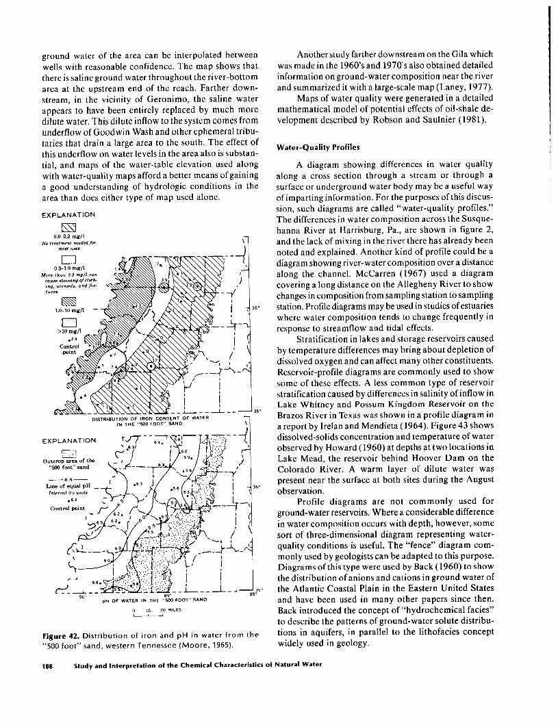
ground water of the area can be interpolated between wells with reasonable confidence. The map shows that there is saline ground water throughout the river-bottom area at the upstream end of the reach. Farther downstream, in the vicinity of Geronimo, the saline water appears to have been entirely replaced by much more dilute water. This dilute inflow to the system comes from underflow of Goodwin Wash and other ephemeral tribu- taries that drain a large area to the south. The effect of this underflow on water levels in the area also is substantial, and maps of the water-table elevation used along with water-quality maps afford a better means of gaining a good understanding of hydrologic conditions in the area than does either type of map used alone.

EXPLANATION

EXPLANATION rsy--,

a outcrop area of the

“500 foot” sand

Figure 42. Distribution of iron and pH in water from the

“500 foot” sand, western Tennessee (Moore, 1965).

Another study farther downstream on the Gila which was made in the 1960’s and 1970”s also obtained detailed information on ground-water composition near the river and summarized it with a large-scale map (Laney, 1977).

Maps of water quality were generated in a detailed mathematical model of potential effects of oil-shale development described by Robson and Saulnier (1981).

Water-Quality Profiles

A diagram showing differences in water quality along a cross section through a stream or through a surface or underground water body may be a useful way of imparting information. For the purposes of this discussion, such diagrams are called “*water-quality profiles.” The differences in water composition across the Susque- hanna River at Harrisburg, Pa., are shown in figure 2, and the lack of mixing in the river there has already been noted and explained. Another kind of profile could be a diagram showing river-water composition over a distance along the channel. McCarren (1967) used a diagram covering a long distance on the Allegheny River to show changes in composition from sampling station to sampling station. Profile diagrams may be used in studies of estuaries where water composition tends to change frequently in response to streamflow and tidal effects.

Stratification in lakes and storage reservoirs caused by temperature differences may bring about depletion of dissolved oxygen and can affect many other constituents. Reservoir-profile diagrams are commonly used to show some of these effects. A less common type of reservoir stratification caused by differences in salinity of inflow in Lake Whitney and Possum Kingdom Reservoir on the Brazes River in Texas was shown in a profile diagram in a report by Irelan and Mendieta (1964). Figure 43 shows dissolved-solids concentration and temperature of water observed by Howard (1960) at depths at two locations in Lake Mead, the reservoir behind Hoover Dam on the Colorado River. A warm layer of dilute water was present near the surface at both sites during the August observation.

Profile diagrams are not commonly used for ground-water reservoirs. Where a considerable difference in water composition occurs with depth, however, some sort of three-dimensional diagram representing water- quality conditions is useful. The “fence” diagram commonly used by geologists can be adapted to this purpose. Diagrams of this type were used by Back (1960) to show the distribution of anions and cations in ground water of the Atlantic Coastal Plain in the Eastern United States and have been used in many other papers since then. Back introduced the concept of “hydrochemical facie? to describe the patterns of ground-water solute distributions in aquifers, in parallel to the lithofacies concept widely used in geology.


wsp 2254 - usgs · these developments have both positive and negative effects on accuracy of the...

Documents