wps3935-ie - world banksiteresources.worldbank.org/extgovanticorr/resources/3035863... · section 3...

IMPACT EVALUATION SERIES NO. 4

EMPOWERING PARENTS TO IMPROVE EDUCATION:

EVIDENCE FROM RURAL MEXICO

Paul Gertler

Harry Patrinos

Marta Rubio-Codina†

Abstract: Mexico’s compensatory education program provides extra resources to primary schools that enroll disadvantaged students in highly disadvantaged rural communities. One of the most important components of the program is the school-based management intervention known as AGEs. The impact of the AGEs is assessed on intermediate school quality indicators (failure, repetition and dropout), controlling for the presence of the conditional cash transfer program. Results prove that school-based management is an effective measure for improving outcomes, based on an over time difference-in-difference evaluation. Complementary qualitative evidence corroborates the veracity of such findings.

JEL Codes: I20, I21, I28

Keywords: School-based management, impact evaluation, Mexico

World Bank Policy Research Working Paper 3935, June 2006 The Impact Evaluation Series has been established in recognition of the importance of impact evaluation studies for World Bank operations and for development in general. The series serves as a vehicle for the dissemination of findings of those studies. Papers in this series are part of the Bank’s Policy Research Working Paper Series. The papers carry the names of the authors and should be cited accordingly. The findings, interpretations, and conclusions expressed in this paper are entirely those of the authors. They do not necessarily represent the views of the International Bank for Reconstruction and Development/World Bank and its affiliated organizations, or those of the Executive Directors of the World Bank or the governments they represent.

† Contact information: Paul Gertler, Haas School of Business, University of California at Berkeley and the World Bank; [email protected], Harry Patrinos, The World Bank; [email protected], Marta Rubio-Codina, University of Toulouse (GREMAQ, INRA), [email protected]. We thank Halsey Rogers and participants at the World Bank AAA decision meetings for useful comments and suggestions. For providing data and institutional knowledge, we are grateful to Felipe Cuellar, Narciso Esquivel, José Carlos Flores, and Miguel Ángel Vargas at CONAFE; Alejandra Macías and Iliana Yaschine at OPORTUNIDADES; and Edgar Andrade at INEE.

WPS3935-IE

1 Introduction

Starting in the United States, the United Kingdom, Australia and Canada, the

decentralization of administrative responsibilities and levels of authority to the school level is a

form of educational reform that has been gaining increasing support in developing countries.

School-based management (SBM) programs – also known as school autonomy reform programs

or school improvement programs – are currently being implemented in a number of countries,

including Hong Kong (China), Indonesia, El Salvador, Nicaragua, Kenya, Kyrgyz Republic,

Nepal, Paraguay and Mexico. They consist in shifting responsibility and decision-making to

school actors: principals, teachers, parents, sometimes even students, and possibly other school

community members (school councils).

The usual argument supporting the implementation of SBM programs is that they may be

a low cost way of improving the efficiency of public spending on education to improve learning

outcomes. The argument is analogous to the basic ideas favoring the decentralization of public

services. Decentralization provides a more efficient and better tailored delivery of services given

that it minimizes information asymmetries concerning tastes, improves the incentives scheme to

provide the good, and reduces the top-down decision-making structure, thus increasing political

accountability. Similarly, SBM initiatives give power to the end users of the service. This

“voice” of the local agents creates a “pressure” to influence and alter school management and

change the form of decision-making to favor students. This eventually leads to a better and more

conducive learning environment for the students and improves learning outcomes.

Analogically, empowerment of the local agents might entail the same deficiencies in

service delivery as those associated with the decentralization of public services: degradation in

service provision. Resources might be misallocated given the increased scope for capture of

resources by the local agents, or because they lack the technical abilities to provide the service or

fail to internalize the positive externalities derived from its provision (Galiani et al 2005). It is

thus crucial for the government to design incentives systems that will minimize the potential for

conflicting interests and opportunistic behavior once decentralization is in place. This is why

SBM programs empower school-level actors conditional upon conformance to a set of centrally

determined operational policies. Moreover, there is substantial variation across interventions

both in terms of the identity of the empowered agents and the level of shifted responsibility.

2

In 1992, the Mexican Government began a process of decentralization of educational

services from the federal to the state level, the “National Agreement for the Modernization of

Basic Education”. A number of reform measures at the central and state levels were implemented.

Among others, these included the advancement of legally supported parental participation in

schools and the development of innovative supply-side interventions to promote education. Some

of these initiatives, like the Quality Schools Program (Programa Escuelas de Calidad, PEC)

launched in 2001, started as pure SBM interventions. Others, like the Compensatory Education

Program –initiated in 1992, combined an SBM component with other more common input

provision interventions. The SBM component of the Compensatory Education Program –the

Support to School Management (Apoyo a la Gestión Escolar) or AGEs, started only in 1996 and

consists of monetary support and training (Capacitación a la Gestión Escolar, CAPAGES) to

Parent Associations (Asociaciones de Padres de Familia, APFs). The APF can spend the money

on the educational purpose of their choosing although spending is limited to small civil works and

infrastructure improvements. Despite being a limited version of SBM, the AGEs represent a

significant advance in the Mexican education system, where parent associations have tended to

play a minor role in school decision-making. AGEs increase school autonomy through improved

mechanisms for participation of directors, teachers and parents’ associations in the management

of the schools. In 2005 more than 45 percent of primary schools in Mexico had an AGE.

In this paper, we examine the impacts of the AGEs on intermediate school quality

indicators (grade failure, grade repetition and intra-year dropout) on the sample of rural general

primary schools that received AGEs support from 1998 onwards. These schools are located in

highly disadvantaged areas and present educational outcomes below the national average. We

exploit the gradual phasing-in of the AGEs intervention over time to identify difference-in-

difference average treatment estimate effects. Results prove that the AGEs are an effective

measure for improving outcomes, grade failure and grade repetition in particular, even after

controlling for the presence of other educational interventions. Qualitative work consisting of

discussions with parents, teachers and school directors in beneficiary and non-beneficiary schools

corroborate the quantitative findings.

The remainder of the paper is organized as follows. The next section reviews the existing

literature on SBM. Section 3 describes the Mexican Compensatory Program and its SBM

component, the AGEs, in greater detail. In Section 4 we discuss the data and expose the

identification strategy used. Results and a discussion of potential biases are provided in sections 5

3

and 6. Section 7 provides a summary of the qualitative interviews assessment. Section 8

concludes.

2. School-Based Management (SBM): A Deeper Look

SBM is the decentralization of levels of authority to the school level. Responsibility and

decision-making over school operations is transferred to school-level actors, which in turn have to

conform to, or operate within a set of centrally determined policies. SBM programs can take on

many different forms, both in terms of who has the power to make decisions as well as the degree

of decision-making devolved to the school level. While some programs transfer authority to

principals or teachers only, others encourage or mandate parental and community participation,

often in school committees (sometimes known as school councils). In general, SBM programs

transfer authority over one or more of the following activities: budget allocation, hiring and firing

teachers and other school staff, curriculum development, textbook and other educational material

procurement, infrastructure improvement, setting the school calendar to better meet the specific

needs of the local community, and monitoring and evaluation of teacher performance and student

learning outcomes. SBM also includes school-development plans, school grants, and sometimes

information dissemination of results (otherwise known as “report cards”).

The goals of programs vary, though they typically involve: (i) increasing the participation

of parents and communities in schools, (ii) empowering principals and teachers, (iii) building

local level capacity, and, perhaps most importantly, (iv) improving quality and efficiency of

schooling, thus raising student achievement levels. Advocates of SBM assert that it should

improve educational outcomes for a number of reasons. First, it improves accountability of

principals and teachers to students, parents and teachers. Accountability mechanisms that put

people at the center of service provision can go a long way in making services work and

improving outcomes by facilitating participation in service delivery. Second, it allows local

decision-makers to determine the appropriate mix of inputs and education policies adapted to

local realities and needs.

The implied benefits of such a system are tremendous with only marginal costs. Among

the benefits are included: increased resources from parents, such as time and in-kind

contributions; more effective use of resources since the site-based actors know more about where

the real need of resources exists; higher school “quality” as a result of efficient use of resources,

and more welcoming school climate since most of the community is involved in management;

4

and increased performance of the students as a result of reduced repetition and dropout rates and

eventually improved learning outcomes. The supposed costs are: payments for school

committees’ time (sometimes); extra resources to be managed at the school level, which also

creates extra work burden for teachers and principals; and parents’ and teachers’ time for

administration, which might be a significant cost for low-income parents who might have to

forego some wage-earning work time to be involved in school committees.

There are a variety of programs under the rubric of SBM, and the literature is

voluminous. Yet rigorous impact evaluations are rare. Summers and Johnson (1994) review the

evidence on the effects of SBM in the United States. In developing countries, evaluations of SBM

programs offer mixed evidence of impacts. El Salvador’s EDUCO (Educación con participación

de la comunidad) program gives parent associations the responsibility for hiring, monitoring and

dismissing teachers. In addition, the parents are also trained in school management, as well as on

how to help their children with school work. Despite rapid expansion of EDUCO schools,

education quality was comparable to traditional schools. In fact, parental participation was

considered the principal reason for EDUCO’s success (Jimenez and Sawada 1999, 2003).

Nicaragua’s Autonomous School Program gives school-site councils –comprised of teachers,

students and a voting majority of parents– authority to determine how 100 percent of school

resources are allocated and to hire and fire principals, a privilege that few other school councils in

Latin America enjoy. Two evaluations found that the number of decisions made at the school

level contributed to better test scores (King and Ozler 1998; Ozler 2001).

In the case of Mexico, only one evaluation exists on the urban pilot of the PEC (Quality

Schools Program) intervention. Using a panel of 74,700 schools and propensity score matching

to create a control group, Shapiro and Skoufias (2005) used difference-in-differences models to

estimate the impact of PEC on dropout, repetition and failure rates. They found that participation

in PEC significantly decreases dropout rates by 0.22 percentage points, failure rates by 0.20

percentage points and repetition rates by 0.28 percentage points. These estimated impacts were

not sensitive to whether participation in PEC was measured as receiving PEC grants for all or for

any one of the three school years covered by the study.

3. The Mexican Compensatory Programs and the AGEs Component

In the early 1990s the National Council of Education Promotion (Consejo Nacional de

Fomento Educativo, CONAFE), a division of the Mexican Secretariat of Public Education

5

(Secretaría de Educación Pública, SEP) started to implement the Compensatory Programs on

behalf of SEP.1 The Compensatory Programs aim to increase the supply and improve the quality

of education in schools with the lowest educational performance levels in highly disadvantaged

communities. The intervention channels extra monetary and in-kind resources to the state

governments. It now serves about five million students in initial, preschool and primary

education, and about 300,000 students in telesecundaria education (lower secondary schooling

imparted by satellite and television), in 29,534 schools in marginalized rural and urban areas in

all 31 states in Mexico.

Since its beginning, CONAFE has received substantial funding from international

agencies to help finance the compensatory program. The World Bank’s Basic Education

Development Loan (PAREIB, 1998-2006) provides a nominal total of $625 million to support the

intervention. Previously, the World Bank had already operated several similar loans between

1991 and 1998 and the Inter-American Development Bank had operated the PIARE intervention

(1995-2000). These loans provided a nominal total of nearly $2 billion dollars between 1991 and

20032. CONAFE’s real costs, despite having grown in the last decade, now are just over $50 per

student per year on average, an extremely low cost compared to a typical cost of $527 per

telesecundaria student and $477 per general middle school student (Shapiro and Trevino 2004).

3.1 Evolution of the Compensatory Programs: Targeting and Phasing-in

Since their start in 1991, the Compensatory Programs have substantially evolved and

expanded their coverage, both to new geographical areas and to new school levels. From 1991-

1996, the Program to Abate Educational Lag (Programa para Abatir el Rezago Educativo,

PARE) operated exclusively in all indigenous and general primary schools in rural localities in

the four states with the highest incidence of poverty: Oaxaca, Guerrero, Chiapas and Hidalgo. In

1993, the Program to Abate Basic Education Lag (Programa para Abatir el Rezago en Educación

Básica, PAREB) included all general and indigenous primary schools in the poorest and

educationally worst performing municipalities in the next ten poorest states, according to the

National Council Population’s (Consejo Nacional de Población, CONAPO) marginality index.

Simultaneously, the Project for the Development of Initial Education (Proyecto para el

1 CONAFE also operates a community education program that leads instruction in highly isolated areas with very few children in school age. Since we only examine CONAFE’s Compensatory Programs, subsequent mention of CONAFE will exclusively refer this intervention unless otherwise noted. 2 Costs are expressed in 2002 US dollars, using an exchange rate of 9.74 Mexican pesos to the dollar.

6

Desarrollo de la Educación Inicial, PRODEI) started to support initial education in the 14 states

attended by PAREB.

In 1995 the Integrated Program to Abate Educational Lag (Programa Integral para

Abatir el Rezago Educativo, PIARE) consolidated the actions enhanced by both initial and basic

education compensatory programs. It extended coverage to all indigenous primary schools and

general primary schools with first year repetition rates above the state average in the next nine

poorest states. In 1998, the PIARE was extended to the eight remaining Mexican states (PIARE-

8). Worst performing schools in the PIARE-8 states were selected according to a targeting index

constructed by CONAFE on the basis of: (i) CONAPO’s community marginality index; (ii)

teacher-student ratios; (iii) the number of students per school; and (iv) educational outcomes. All

general primary schools falling in the third and fourth quartiles of the targeting index were

selected as beneficiary schools. As in previous stages, all indigenous primary schools were

automatically attended.

Finally, in 1998 and in order to integrate all previous Compensatory Programs and to

provide integrated and continuous educational support to all children ages 0 to 14, the Program to

Abate Educational Lag in Initial and Basic Education (Programa para Abatir el Rezago

Educativo en Educación Inicial y Básica, PAREIB) was established. PAREIB targets for the first

time pre-schools, general and technical junior high schools, and telesecundarias. It also extended

its coverage to marginalized semi-urban and urban areas. General primary schools were targeted

using the same criteria applied to target PIARE-8 schools. These were also extended to pre-

school and junior high schools.3 Schools offering any form of indigenous or community

education were automatically targeted. The PAREIB is the only Compensatory Education

Program currently functioning.

3.2 Components of the Compensatory Programs

CONAFE’s compensatory programs do not operate schools, but rather give extra support

to all indigenous schools, and targeted primary and secondary schools. By design, the

interventions and supports given have varied across school types and along the different program

phases. Moreover, the final decision to allocate resources depends on the state government and is

based on the school needs and on the availability of resources in each state. As a consequence,

3 Section 4.2 further details the targeting methodology applied to select beneficiary schools.

7

there is a substantial variation in the type, number and timing of interventions each attended

school receives.

By 1996 the number of interventions was reorganized and limited to the improvement

and/or building of school infrastructure facilities, the provision of school equipment and supplies,

pedagogical training for teachers, institutional strengthening, incentives to monitors (school

supervisors), and performance based monetary incentives to teachers in multiple grade schools

and in schools with more than six teachers. Starting in 1996, CONAFE introduced the support to

school management component, the AGEs, which is the focus of this study. The AGEs financial

support consists of quarterly transfers to APF school accounts, varying from $500 to $700 per

year according to the size of the school. The use of funds is specified in the Operational Manual

of the project and is subject to annual financial audits for a random sample of schools. Among

other things, the parents are not allowed to spend money on wages and salaries for teachers.

Most of the money goes to infrastructure improvements and small civil works. The intervention

was complemented, starting in 2003, with a training component (CAPAGEs) aimed at guiding

parents in the management of the school funds transferred through the AGES. The CAPAGEs

also provides parents with participatory skills to increase their involvement in school activities,

and with information on achievement of students and ways in which parents can help improve

their learning.4

3.3 Existing Evidence on the Impact of Compensatory Education

Results from previous Government supported evaluations show a significant impact of

CONAFE in lowering the probability that school average repetition rates increase between 1998-

99 and 2001-02 in rural primary schools (Benemérita Universidad Autónoma de Puebla 2004).

External evaluations show significant increases in Spanish test scores for indigenous students

(López-Acevedo 2002). The author compares CONAFE (PARE) -supported schools between the

school years 1992-93 and 1994-95 with comparable schools in the state of Michoacán that were

not receiving the support at the time. The evaluation concluded that the PARE program could

result in increases of 45 to 90 percent on indigenous student performance, and of the order of 19

to 38 percent on aggregate rural school performance. A complementary evaluation by Paqueo and

López-Acevedo (2003) used the same methodology to study the differential effects of CONAFE’s

4 The AGEs component does not operate in telesecundarias. Although CONAFE is supposed to provide audiovisual materials and infrastructure improvements to all telesecundaria schools; in practice, the intervention has so far been limited to the delivery of one or two computers per intervened telesecundaria.

8

PARE intervention on sixth graders’ Spanish test scores between the poorest and the least poor

children in indigenous and rural schools. The authors found that the poorest students benefited

less from the intervention than the not so poor students. These findings raise the question of

whether the very poor are able to fully take advantage of new opportunities in the form of school

quality improvements as their ability might be compromised by malnutrition and lack of brain

stimulation at early life stages.

More recently, Shapiro and Moreno (2004) conducted an impact evaluation of the

PAREIB intervention on Spanish and math test scores at both the primary and junior-high school

levels. Using propensity score matching techniques on student background data, the authors find

that CONAFE is effective in improving primary school math learning and junior-high school

Spanish learning. CONAFE also seems to lower primary school repetition and failure rates. They

conclude that while CONAFE seems to improve short term educational outcomes the

improvement varies by subject of instruction and student demographics.

Evaluations of specific components in CONAFE-implemented compensatory program do

not yet exist.5 This paper, while contributing to the nascent literature on the effects of SBM

interventions on educational outcomes, also fills the existing gap in the evaluation of CONAFE’s

Compensatory Programs.

4. Estimation and Identification

Our objective is to estimate the impacts of the SBM support component of the

Compensatory Education Program – the so-called AGEs – on intermediate indicators of student

performance and school quality, namely failure, repetition and (intra-year) dropout rates.6 We

specifically focus on the impact of the AGEs support between 1998 and 2001. These years

correspond to stages PIARE-8 and PAREIB (Phase I) of the CONAFE intervention. Section 4.1

lays out the econometric specification; section 4.2 describes the data; finally, we discuss and

validate the identifying assumptions in section 4.3.

5 In previous work on the joint evaluation of the impacts of the Compensatory Programs (supply-sided intervention) and the Oportunidades scholarships (demand-sided intervention) on schooling outcomes, (Gertler et al 2006), we decomposed the CONAFE implemented intervention in its different components, for the first time. Our findings motivated the direction of the current piece of research. 6 Ideally, we would like to use test score data as a more direct measure of student performance. However, standardized national assessments (Estándares Nacionales) were collected on a sample representative of all schools (from all geographical and social strata) in Mexico. The sample of schools common to both the CONAFE and the Estándares Nacionales datasets is too small to perform the analysis on test score data.

9

4.1 Econometric Specification

Let us assume that the probability that student i in school s at time t attains educational

outcome Yist=Y is a function of: the presence (or the lack) of the AGEs support in the school

during the previous school year, 1, −tsAGEs ={0,1}; the student’s i vector of j individual

characteristics, Iisjt, such as her ability, skills and family background; and the k-th vector of

school’s s characteristics, including school quality and all other educational interventions

received at the school level during the previous year, Xskt. More formally,

),,()( 1, sktisjttsist XIAGEsfYYpr −== (1)

We consider three different educational outcomes: the probability that the student fails an

exam (Fist = F), repeats a grade (Rist =R) or drops out of school during the school year t (Dist =D).

Unfortunately, we do not have individual (student) measures of performance but rather school

aggregate measures, so we are not able to estimate (1) directly. However, assuming that f(.) is a

linear function, we can obtain the average rate of success/failure at the school level by adding up

the student individual probabilities by school and normalizing them by the number of students in

each school, Nst. Then, equation (1) re-writes:

),,()( 1, sktsjttsst XIAGEsfYpr −= (2)

where ∑=

=N

iist

st

st YN

Y1

1 represents the school average failure rate, repetition rate or dropout rate at t;

and ∑=

=N

iisjt

st

sjt IN

I1

1 , the vector of the j school-averaged student characteristics.

In order to evaluate the impact of the AGEs component on school averaged student

performance, we estimate the following reduced form for all t =1997-2001 that follows from (2):7

∑∑=

− ++++++=K

kstsktkts

tstlttsst XAGEsPOTAGEstrendY

21,11 * εββπξηα (3)

where sα and tη are school and time fixed effects; ltξ are state specific time dummies intended

to capture state specific aggregate time effects correlated with schooling outcomes (demographic

trends or changes in government, for example). POTAGEss is a dichotomous variable equal to 1

if the school s is a potential treatment school; this is to say, if s will receive the AGEs support

7 We take school year 1997-98 as the baseline year. Evaluation years are from school year 1998-99 to school year 2001-02.

10

(POTAGEss =1) for some (or all) of the treatment years (t =1998-2001). Thus, the term trend*

POTAGEss is the time trend specific to potential AGEs-treatment schools, and attempts to control

for the different evolutions that schools that receive and that do not receive AGEs might have

experienced over time. The dummy AGEss,t-1 takes on the value of one if the school has received

the AGEs support during school year t-1. Then, 1β̂ is the difference-in-difference estimate of the

one period lagged effect of the presence of AGEs in the school on educational outcomes. More

specifically, it measures changes in school-averaged student performance trends between early

intervened schools (treatments) and latter intervened or not yet intervened schools (controls).

Note that we are explicitly assuming that the AGEs support requires some time – a full school

year at least, to be effective. Thus, we take educational outcomes at the end of the school year (at

t) and run them as a function of the school receiving the AGEs support for, at least, the entire

school year; this is to say, starting at t-1. Xskt is the vector of current school characteristics and

education related interventions received during the year previous to that of analysis that we

describe below. ∑=

=N

iist

st

stN 1

1 εε is the school averaged individual error terms that includes all the

unobserved individual characteristics (learning ability, disutility from studying, etc.) that we

assume uncorrelated with the explanatory variables for the time being.8 We compute robust

standard errors clustered at the school level to correct for heteroskedasticity and serial correlation.

Because of the inclusion of school fixed effects, all time invariant school observed and

unobserved characteristics that could be correlated with both school outcomes and program

placement are controlled for.

The vector of school characteristics includes the school student-to-teacher ratio, and the

average number of students per class (crowding index).9 With regards to alternative public

policies directed to improve schooling quality and accessibility, we specifically control for: the

ratio of Oportunidades beneficiary students in the school, which is a measure of the intensity of

the Oportunidades program in the school – on the demand side; and the proportion of teachers

8 The intervention might alter the number of children enrolling in school. If as a consequence the distribution of students’ skills changes in treatment schools (with respect to control schools), then the program impact estimates are likely to be biased. We will explore the existence of this bias in section 6. The characteristics of the average student in the school sjtI are also included in the error term because of lack of data on individual students’ characteristics. 9 Missing values for school characteristics (but not school education interventions) have been replaced by the time specific municipality (or state, if the value was still missing) average. We include indicator variables to account for the replacement. The School Census – described below, also collects data on the number of classrooms, desks, habilitated workshop and lab areas, etc. Unfortunately, these variables did not vary enough over time to be included as additional controls.

11

under Carrera Magisterial, and the reception of other (sporadic) CONAFE supported

interventions – on the supply side.

Oportunidades, formerly known as Progresa, combines a traditional cash transfer

program with financial incentives for families to invest in the human capital of their children.

Program benefits include cash transfers that are disbursed conditional on the household engaging

in a set of behaviors designed to improve health and nutrition (preventive checkups, prenatal care,

and health and hygiene education) and on school aged children attending school. The size of the

cash transfer is large, corresponding on average to about one-third of household income for the

beneficiary families. Another unique feature of the program is that the cash transfers are given to

the mother of the family, a strategy designed to target the funds within the household to

improving the children’s education and nutrition. See Skoufias (2005) for a review of evaluations

on the program impacts. Carrera Magisterial was launched in the 1990s. In that program

principals, along with teachers and teacher aides, voluntarily participate in a year-long assessment

process that awards 100 points for education, experience and other factors. Each principal

receives up to 20 points based on the mean test scores of her school’s students and teachers in

standardized assessments. In recent years, principals scoring above a nationally-specified cut-off

score (70) have a sharply higher probability of receiving an award. The awards are substantial -

more than 35 percent of the principal’s annual wage, and they persist for their entire career.

Since 1993, close to 85,000 principals have been awarded the lowest level of promotion, and

several hundred thousand more have received promotions to even higher (and more lucrative)

levels. For an evaluation, see McEwan and Santibañez (2005).

As previously noted, the CONAFE intervention is composed of several different

interventions besides the AGEs monetary support. These include: provision of school and student

teaching and learning supplies (textbooks, notebooks, pencils and pens), teacher training,

improvement of existing or building of new facilities, provision of equipment (desks, bookcases,

typewriters, etc.) and performance based incentives to teachers. Depending on the econometric

specification, we explicitly control for the presence of these interventions in the school.

4.2 Data Sources and Sample Sizes

We use administrative data on CONAFE coverage from 1991 to 2003 to identify AGEs

beneficiary schools and schools receiving any of the other CONAFE supported interventions. We

use data from the Mexican School Census (Censo Escolar), an annual listing of background and

12

outcome data for all schools in Mexico to measure failure, repetition and intra-year dropout.10

Data on the number of Oportunidades beneficiary students in each school comes from

administrative Oportunidades coverage data from 1997 to 2003. All school data sources are

combined at the school level thanks to a unique school identifier code. We also take advantage of

the Mexico’s 1990 and 2000 Population Census and the 1995 Conteo to construct socioeconomic

locality indicators that will help identify the evaluation subsample. This data is combined with

the school level data using locality identifier codes.11

The set of AGEs treatment schools is defined as the set of schools that started receiving

the AGEs monetary support in the beginning of any school year between the school years 1998-

99 and 2001-02, and that received it continuously ever since. The comparison group consists of

those schools that started receiving the AGEs allowance from school year 2002-03 onwards. In

some cases and because we only have coverage data until school year 2003-04 some of the

schools included in the control group might not have yet received treatment. Ideally, this group

of control schools would only differ from the group of treatment schools in their treatment status.

However, given CONAFE’s phasing-in criteria (CONAFE targeted indigenous schools, and

schools in poorer and higher marginalized areas first), this is unlikely to be the case and less so if

indigenous areas are systematically different from non-indigenous (Ramirez 2006). In order to

achieve well-balanced (comparable) samples, we restrict our study to the balanced panel of 6,038

rural non-indigenous primary schools observed continuously between 1995 and 2003.12 Out of

these, 2,580 (42.7 percent) are AGEs treatment schools, and the remaining 3,258 (57.3 percent)

are AGEs control schools (see Table 1). Table 1 also shows the number of schools that started

receiving AGEs by school year. For all these schools we know the value of the targeting index

computed by CONAFE in 2000.

10 The information in the School Census also allows computation of inter-year dropout rate. However, because it is impossible to distinguish between students that are purely dropping out of the educational system or merely changing schools, we chose to work with intra-year dropout rates – where the potential of error measurement is arguably smaller. 11 For a non-negligible number of localities, locality and municipality codes as registered in the Population Census have changed over time. This prevents following these localities through time. To construct locality level indicators, we take the 2000 Census as the reference year and keep only those localities whose identifying codes have remained the same. 12 To allow comparison across outcomes, the analysis sample is restricted to those schools with non-missing observations for any of the dependent variables studied. Results are robust to the inclusion/exclusion of schools with missing information for one or more of the outcome variables. We have also dropped out of the sample schools with extremely high numbers of students and/or teachers (top 0.5 percent of each distribution).

13

1998 1999 2000 2001 2002 2003 After Total

Number of Schools by Phase In Date72

(1.19)801

(13.27)1,084

(17.95)623

( 10.32 )3,173

(52.55 ) 53

(0.88)232

(3.84)

Number of Schools by Treatment Status

Table 1: Sample Sizes and Number of Schools Phased into AGEs by Year -Subsample of General Rural Primary Schools

Date school starts receiving AGEs SupportAGEs Treatment Schools AGEs Control Schools

AGEs treatment schools are schools that continuously receive the Apoyo a la Gestión Escolar (AGEs),starting in 1998 (or later) until 2001.

2,580 ( 42.73 )

3,458 ( 57.27)

6,038(100)

The 2000 targeting index was constructed by CONAFE as a tool to select the worst

performing schools in less marginalized states to be targeted by PAREIB. It used 2000 Census

data on localities and School Census data for the school year 1999-2000 on school characteristics

(student density, student teacher ratio, etc.) and educational outcomes (failure, repetition and

school dropout).13 The targeting rule applied implied that (i) all rural schools in highly

marginalized areas and (ii) all schools falling in the third and fourth quartiles of the targeting

index in less marginalized areas would be selected as CONAFE beneficiaries starting in 2001. As

in previous stages of the program, all indigenous primary schools were automatically selected.

We basically exploit the index as a way of testing for balance between the constructed treatment

and control groups of schools: schools with similar targeting indexes are likely to have similar

values of the variables used in its construction. Hence, they are likely to be in similar

environments and have similar educational outcomes. We also use the index to define different

samples on which we check the robustness of the results found. Figure 1 shows that the index

distributions for treatment and control schools overlap over the entire support.14

13 See CONAFE (2000) for more details on the weighting of variables and construction of the targeting index. A previous index that used 1995 Census data and 1995-96 School Census data was constructed to target PIARE-8 schools. Unfortunately, we could only find data on this index for urban schools. 14 At first, it might seem surprising the fact that the distribution of treatment schools (targeted at earlier stages because of larger index values; that is, lower efficiency levels) is more to the left than the distribution of control schools. Recall nonetheless, that this index was computed when most treatment schools had already been under treatment for a year or two, and therefore had had time to improve their educational outcomes with respect to control schools.

14

0.2

.4.6

Den

sity

4 6 8 10 12Targeting Index

CONAFE Treatment Schools CONAFE Control Schools

CONAFE Treatment and CONAFE Control SchoolsFigure 1: Distribution of the 2000 Targeting Index

Means and standard deviations for a few school observable characteristics and for the

dependent variables in 1997 (baseline), across AGEs treatment and AGEs control schools, are

shown in Table 2. Summary statistics on the intensity of the different education interventions

across treatment years is also shown. Schools in the sample have, on average, 132 students, 7

classrooms and between 4 and 5 teachers. AGEs treatment schools are smaller on average: they

have less students and teachers, and lower student teacher ratios and crowding indexes. The

failure rate is 10 percent in both types of schools. However, while repetition rates are larger in

AGEs treatment schools (9.6 versus 9.2 in control schools), intra-year dropout is 0.4 points lower

in treatment schools (3.8 percent in treatment schools versus 4.2 percent in control schools). This

might reflect a higher mobility and school turnover in larger towns, where schools are more

unlikely to receive AGEs. Control schools have a larger proportion of teachers in Carrera

Magisterial but a significantly lower share of Oportunidades students. This is suggestive of a

relatively high degree of overlap between CONAFE and Oportunidades, which is not at all

surprising given that both interventions are targeting schools and populations in highly

disadvantaged areas. Moreover, schools that do not receive AGEs are significantly less likely to

receive any of the other CONAFE supported interventions, which suggests a high prevalence of

AGEs support amongst CONAFE schools.

15

Table 2: Descriptive Statistics by Treatment Status -Subsample of General Rural Primary Schools

N Mean SDDependent Variables at Baseline (1997)

Failure Rate 6038 0.100 (0.058)Repetition Rate 6038 0.093 (0.056)Intra-Year Drop Out Rate 6038 0.040 (0.045)

School Characteristics at Baseline (1997)Number of Teachers 6038 4.889 (3.504)Number of Desks 6034 79.785 (86.755)Number of Classrooms 6038 6.946 (2.215)Student-Teacher Ratio 6038 26.381 (7.671)Class Crowding Index 6038 24.729 (8.727)Total Enrollment 6038 132.217 (111.839)

Other Interventions over Treatment Period (1998-2001)Proportion of Teachers in Carrera Magisterial 6038 0.527 (0.363)Proportion of Schools with Infrastructure Support (CONAFE) 6038 0.018 (0.131)Proportion of Schools with Equipment Support (CONAFE) 6038 0.005 (0.074)Proportion of Schools with Teacher Inventives Support (CONAFE) 6038 0.003 (0.053)Proportion of Schools with School Supplies Support (CONAFE) 6038 0.200 (0.400)Proportion of Schools with Teacher Training Support (CONAFE) 6038 0.096 (0.295)Ratio of Oportunidades students in the School 6038 0.253 (0.225)

Dependent Variables at Baseline (1997)Failure Rate 2580 0.100 (0.063)Repetition Rate 2580 0.096 (0.061)Intra-Year Drop Out Rate 2580 0.038 (0.048)



Dependent Variables at Baseline (1997)Failure Rate 3458 0.100 (0.055)Repetition Rate 3458 0.092 (0.051)Intra-Year Drop Out Rate 3458 0.042 (0.042)



AGEs treatment schools are schools that continuously receive the Apoyo a la Gestión Escolar (AGEs),starting in 1998 (or later) until 2001. Schools with extremely high values of the dependent variables have been dropped (top 0.5% of each distribution). Sample restricted to schools with no missing information on any of the dependent variables studied.

All Schools

AGEs Treatment Schools

AGEs Control Schools

16

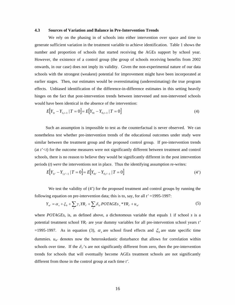
4.3 Sources of Variation and Balance in Pre-Intervention Trends

We rely on the phasing in of schools into either intervention over space and time to

generate sufficient variation in the treatment variable to achieve identification. Table 1 shows the

number and proportion of schools that started receiving the AGEs support by school year.

However, the existence of a control group (the group of schools receiving benefits from 2002

onwards, in our case) does not imply its validity. Given the non-experimental nature of our data

schools with the strongest (weakest) potential for improvement might have been incorporated at

earlier stages. Then, our estimates would be overestimating (underestimating) the true program

effects. Unbiased identification of the difference-in-difference estimates in this setting heavily

hinges on the fact that post-intervention trends between intervened and non-intervened schools

would have been identical in the absence of the intervention:

[ ] [ ]0|0| 1,001,11 =−==− −− TYYETYYE tttt (4)

Such an assumption is impossible to test as the counterfactual is never observed. We can

nonetheless test whether pre-intervention trends of the educational outcomes under study were

similar between the treatment group and the proposed control group. If pre-intervention trends

(at t’<t) for the outcome measures were not significantly different between treatment and control

schools, there is no reason to believe they would be significantly different in the post intervention

periods (t) were the interventions not in place. Thus the identifying assumption re-writes:

[ ] [ ]0|0| 1',0'01',1'1 =−==− −− TYYETYYE tttt (4’)

We test the validity of (4’) for the proposed treatment and control groups by running the

following equation on pre-intervention data; this is to, say, for all t’ =1995-1997:

''

''1'

''' * stt

tstt

ttltsst uYRPOTAGEsYRY ++++= ∑∑ δγξα (5)

where POTAGEss is, as defined above, a dichotomous variable that equals 1 if school s is a

potential treatment school YRt’ are year dummy variables for all pre-intervention school years t’

=1995-1997. As in equation (3), sα are school fixed effects and ltξ are state specific time

dummies. ust’ denotes now the heteroskedastic disturbance that allows for correlation within

schools over time. If the δ.t’’s are not significantly different from zero, then the pre-intervention

trends for schools that will eventually become AGEs treatment schools are not significantly

different from those in the control group at each time t’.

17

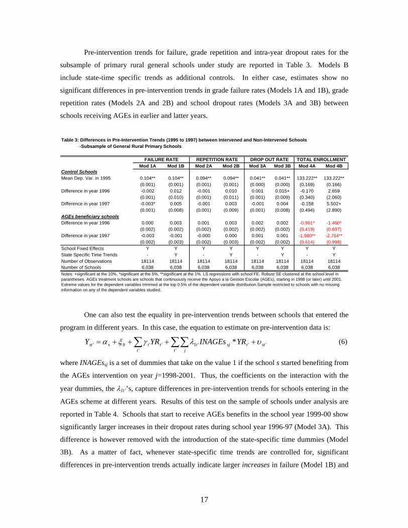
Pre-intervention trends for failure, grade repetition and intra-year dropout rates for the

subsample of primary rural general schools under study are reported in Table 3. Models B

include state-time specific trends as additional controls. In either case, estimates show no

significant differences in pre-intervention trends in grade failure rates (Models 1A and 1B), grade

repetition rates (Models 2A and 2B) and school dropout rates (Models 3A and 3B) between

schools receiving AGEs in earlier and latter years.

Table 3: Differences in Pre-Intervention Trends (1995 to 1997) between Intervened and Non-Intervened Schools -Subsample of General Rural Primary Schools

Mod 1A Mod 1B Mod 2A Mod 2B Mod 3A Mod 3B Mod 4A Mod 4BControl SchoolsMean Dep. Var. in 1995 0.104** 0.104** 0.094** 0.094** 0.041** 0.041** 133.222** 133.222**

(0.001) (0.001) (0.001) (0.001) (0.000) (0.000) (0.169) (0.166)Difference in year 1996 -0.002 0.012 -0.001 0.010 0.001 0.015+ -0.170 2.659

(0.001) (0.010) (0.001) (0.011) (0.001) (0.009) (0.340) (2.060)Difference in year 1997 -0.003* 0.005 -0.001 0.003 -0.001 0.004 -0.158 5.502+

(0.001) (0.008) (0.001) (0.009) (0.001) (0.008) (0.494) (2.890)AGEs beneficiary schoolsDifference in year 1996 0.000 0.003 0.001 0.003 0.002 0.002 -0.961* -1.460*

(0.002) (0.002) (0.002) (0.002) (0.002) (0.002) (0.419) (0.697)Difference in year 1997 -0.003 -0.001 -0.000 0.000 0.001 0.001 -1.980** -2.764**

(0.002) (0.003) (0.002) (0.003) (0.002) (0.002) (0.614) (0.998)School Fixed Effects Y Y Y Y Y Y Y YState Specific Time Trends - Y - Y - Y - YNumber of Observations 18114 18114 18114 18114 18114 18114 18114 18114Number of Schools 6,038 6,038 6,038 6,038 6,038 6,038 6,038 6,038

TOTAL ENROLLMENT

Notes: +significant at the 10%, *significant at the 5%, **significant at the 1%. LS regressions with school FE. Robust SE clustered at the school level in parantheses. AGEs treatment schools are schools that continuously receive the Apoyo a la Gestión Escolar (AGEs), starting in 1998 (or later) until 2001. Extreme values for the dependent variables trimmed at the top 0.5% of the dependent variable distribution.Sample restricted to schools with no missing information on any of the dependent variables studied.

FAILURE RATE REPETITION RATE DROP OUT RATE

One can also test the equality in pre-intervention trends between schools that entered the

program in different years. In this case, the equation to estimate on pre-intervention data is:

''

''1'

''' * stt j

tsjtt

ttltsst YRINAGEsYRY υλγξα ++++= ∑∑∑ (6)

where INAGEssj is a set of dummies that take on the value 1 if the school s started benefiting from

the AGEs intervention on year j=1998-2001. Thus, the coefficients on the interaction with the

year dummies, the λ1t’’s, capture differences in pre-intervention trends for schools entering in the

AGEs scheme at different years. Results of this test on the sample of schools under analysis are

reported in Table 4. Schools that start to receive AGEs benefits in the school year 1999-00 show

significantly larger increases in their dropout rates during school year 1996-97 (Model 3A). This

difference is however removed with the introduction of the state-specific time dummies (Model

3B). As a matter of fact, whenever state-specific time trends are controlled for, significant

differences in pre-intervention trends actually indicate larger increases in failure (Model 1B) and

18

repetition (Model 2B) across AGEs treatment schools. This is suggestive that, if anything schools

that start receiving AGEs in earlier years were experiencing worst dynamics in terms of schooling

outcomes than schools that receive the AGEs support later. Therefore, our estimates are more

likely to underestimate the AGEs effect rather than overestimate it. Given the sets of estimates in

Tables 3 and 4, pre-intervention trends look well-balanced enough overall for endogenous

program placement bias not be a serious threat to identification.15

Mod 1A Mod 1B Mod 2A Mod 2B Mod 3A Mod 3B Mod 4A Mod 4BControl SchoolsMean Dep. Var. in 1995 0.104** 0.104** 0.094** 0.094** 0.041** 0.041** 133.222** 133.222**

(0.001) (0.001) (0.001) (0.001) (0.000) (0.000) (0.169) (0.166)Difference in year 1996 -0.002 0.014 -0.001 0.012 0.001 0.014 -0.170 2.518

(0.001) (0.010) (0.001) (0.011) (0.001) (0.009) (0.340) (2.098)Difference in year 1997 -0.003* 0.006 -0.001 0.004 -0.001 0.003 -0.158 5.259+

(0.001) (0.008) (0.001) (0.009) (0.001) (0.008) (0.494) (2.938)AGEs beneficiary schoolsDifference in year 1996 * AGEs starting in 1998 -0.001 0.001 -0.003 -0.002 0.006 0.009 3.018 0.480

(0.013) (0.013) (0.012) (0.012) (0.009) (0.009) (2.492) (2.926)Difference in year 1996 * AGEs starting in 1999 0.004 0.007+ 0.006+ 0.008* -0.000 -0.001 -0.504 -1.490*

(0.003) (0.004) (0.003) (0.004) (0.003) (0.003) (0.461) (0.640)Difference in year 1996 * AGEs starting in 2000 -0.003 -0.002 -0.004 -0.003 0.002 0.004 -1.254* -1.361

(0.003) (0.003) (0.003) (0.003) (0.002) (0.003) (0.543) (0.936)Difference in year 1996 * AGEs starting in 2001 0.002 0.004 0.002 0.004 0.006** 0.002 -1.499* -1.855*

(0.003) (0.004) (0.003) (0.004) (0.002) (0.003) (0.596) (0.897)Difference in year 1997 * AGEs starting in 1998 -0.006 -0.008 -0.004 -0.006 0.009 0.004 3.270 -0.386

(0.013) (0.013) (0.011) (0.011) (0.011) (0.011) (2.924) (3.650)Difference in year 1997 * AGEs starting in 1999 -0.002 -0.000 0.002 0.003 -0.000 -0.003 -0.774 -2.766**

(0.004) (0.004) (0.004) (0.004) (0.003) (0.003) (0.665) (0.933)Difference in year 1997 * AGEs starting in 2000 -0.005+ -0.003 -0.003 -0.004 0.002 0.003 -2.722** -2.449+

(0.003) (0.003) (0.003) (0.003) (0.002) (0.003) (0.794) (1.301)Difference in year 1997 * AGEs starting in 2001 -0.000 0.002 0.002 0.002 -0.001 0.004 -2.848** -3.671**

(0.003) (0.004) (0.004) (0.004) (0.002) (0.003) (0.949) (1.419)School Fixed Effects Y Y Y Y Y Y Y YState Specific Time Trends - Y - Y - Y - YNumber of Observations 18114 18114 18114 18114 18114 18114 18114 18114Number of Schools 6,038 6,038 6,038 6,038 6,038 6,038 6,038 6,038

TOTAL ENROLLMENT

Table 4: Differences in Pre-Intervention Trends (1995 to 1997) between Non-Intervened Schools and Schools Intervened in Subsequent Years -Subsample of General Rural Primary Schools


FAILURE RATE REPETITION RATE DROP OUT RATE

Identification also relies in the inclusion of school fixed effects that control for biases due

to differences in time-invariant factors across schools. In addition, the state-time dummies are 15 Alternatively we could control for the program phase-in rule as a way of minimizing the potential for endogenous program placement. The many deficiencies associated with this approach dissuaded us from applying it. First, the targeting rule is computed at one point in time. We could construct a time-varying targeting index applying the formula to different years. However, we would need to generate time variation to some variables by extrapolation which might add considerable measurement error. Second and more importantly, the targeting rule for primary schools is not unique. According to CONAFE, schools that were to be phased in under earlier stages (PAREB, PIARE) will continue to respond to the criteria associated with those stages, even if they start receiving benefits at later years. Since we are unable to perfectly assign –given the data available, the correct rule to each school, we chose not to control for the specific targeting rule. In any case, the targeting rule does not determine when schools do receive a particular CONAFE intervention, the AGEs support in this particular case.

19

meant to capture state-specific aggregate time effects that might be correlated with schooling

outcomes: changes in demographic trends in the state that might affect enrollment; or changes in

the state government characteristics, for example, shifts in tastes and priorities about education

that might alter the allocation of resources. Treatment specific time trends are included to capture

the different evolutions treatment and control schools might have experienced over time.

Moreover, we control for other education programs currently operating in the school to avoid

incorrectly attributing effects to the AGEs intervention. In the same spirit, we also use as many

school varying characteristics we are able to construct as controls. Although there are not many,

it seems plausible to assume that schools do not change substantially in the span of 5 years. The

estimate of the treatment effect will be unbiased as long as there are no unobserved time-varying

characteristics or trends correlated with the treatment variables. We discuss potential biases in

section 6.

5. Quantitative Evidence on Failure, Repetition and Dropout

5.1 Graphical Evidence

Albeit limited, graphs can provide suggestive evidence. Figures 2, 3 and 4 present the

evolution of average grade failure, grade repetition and school intra-year dropout rates over time

for AGEs treatment schools (solid line) and AGEs control schools (dashed line). The vertical line

at 1997 marks the beginning of the intervention period.16

Grade failure and grade repetition start being higher for the group of initially treated

schools. Intra-year dropout rates, however, are lower amongst treatment schools all the way

through. By 1997 – the baseline year, the marginally higher average failure rate observed in

treatment schools drops down to the failure rate level of control schools, at exactly 10 percent.

From school year 1999-2000 on, failure and repetition rates for treatment schools fall below those

of control schools. Although the difference is unlikely significant it shows some trend towards

minimizing the gap between AGEs compensated and AGEs non-compensated schools in terms of

intermediate quality of schooling indicators. As a matter of fact, the graphs clearly show a

sharper decrease in failure and repetition rates for treatment schools by the end of school year

1999-2000, when 13.3 percent of the schools have already received the monetary support for a 16 The intervention period starts in school year 1998-99. However, by construction failure and repetition are measured at the end of the school year. Thus, the average failure plotted in t =1998 corresponds to the average failure at the end of the school year 1998-99, once the program has already been in place for an entire school year had it started at the beginning of the school year. Hence, the vertical line separating pre- and post-intervention trends is drawn at t-1 =1997 to graphically depict the school year difference we allow for the intervention to be effective.

20

full school year and an insignificant 1.2 of schools for a couple of years (see Table 1). The plots

do not show any effect concerning intra year dropout rates. Also, note that pre-intervention

trends are rather parallel which graphically supports the validity of the identification strategy.17

.07

.08

.09

.1.1

1Fa

ilure

Rat

e

1995 1996 1997 1998 1999 2000 2001Year

AGEs Treatment AGEs Control

AGEs vs. Non-AGEs SchoolsFigure 2: Failure Rate Trends

.075

.08

.085

.09

.095

Rep

etiti

on R

ate

1995 1996 1997 1998 1999 2000 2001Year


AGEs vs. Non-AGEs SchoolsFigure 3: Repetition Rate Trends

17 The evidence depicted in these graphs is only partial and has to be seen accordingly. They plot raw means for AGEs treatment and AGEs control schools. As such, the effect of any other factors that might be altering the outcome evolution in any way is not netted out in here. Moreover, these graphs do not take into consideration the differences in phase-in of the AGEs support across schools either.

21

.03

.05

.07

Dro

p O

ut R

ate

1995 1996 1997 1998 1999 2000 2001Year


AGEs vs. Non-AGEs SchoolsFigure 4: Drop Out Rate Trends

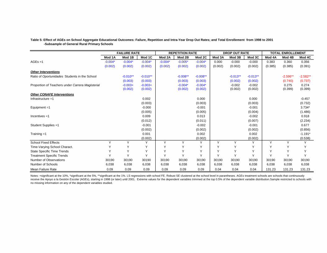
5.2 Average Treatment Effects

Estimates of the average treatment effect in equation (3) between school years 1998-99

and 2001-02 for failure, grade repetition and intra-year dropout rates are presented in Table 5. As

already explained, the school year 1997-98 will act as the pre-intervention year in the

computation of the difference-in-difference treatment estimates. For each dependent variable, the

first column (under Model A) shows the estimated AGEs effect when no other education

intervention is controlled for. In the next column (Model B), we add the proportion of

Oportunidades students in the school and the proportion of teachers under the Carrera

Magisterial scheme as controls. In the last column (Model C) we include additional indicator

variables that control for the existence of any other CONAFE supported intervention. All

regressions include school and time fixed effects, state specific time trends, a treatment specific

trend and all the time varying school characteristics listed above.

Results consistently show a significant effect of AGEs in reducing failure and grade

repetition, which is independent of the inclusion of controls for the other education interventions.

As a matter of fact, the point estimates – of -0.4 percentage points or alternatively, a 4.4 percent

decrease in the proportion of students failing or repeating a grade in the school, practically does

not vary across regressions. This suggests that the effects of the AGEs intervention on failure and

repetition in the first column are not biased because of the coexistence in the school of other

Mod 1A Mod 1B Mod 1C Mod 2A Mod 2B Mod 2C Mod 3A Mod 3B Mod 3C Mod 4A Mod 4B Mod 4CAGEs =1 -0.004* -0.004* -0.004* -0.004* -0.005* -0.004* 0.000 -0.000 -0.000 0.383 0.360 0.356

(0.002) (0.002) (0.002) (0.002) (0.002) (0.002) (0.002) (0.002) (0.002) (0.385) (0.385) (0.391)

Other InterventionsRatio of Oportunidades Students in the School -0.010** -0.010** -0.008** -0.008** -0.013** -0.013** -2.596** -2.582**

(0.003) (0.003) (0.003) (0.003) (0.002) (0.002) (0.740) (0.737)Proportion of Teachers under Carrera Magisterial -0.003+ -0.003+ -0.004* -0.004* -0.002 -0.002 0.275 0.274

(0.002) (0.002) (0.002) (0.002) (0.002) (0.002) (0.399) (0.399)

Other CONAFE InterventionsInfrastructure =1 0.002 0.000 0.000 -0.457

(0.003) (0.003) (0.003) (0.732)Equipment =1 -0.000 -0.001 -0.001 3.734*

(0.005) (0.005) (0.004) (1.486)Incentives =1 0.009 0.013 -0.002 0.918

(0.012) (0.011) (0.007) (2.234)Student Supplies =1 -0.001 -0.002 -0.001 0.677

(0.002) (0.002) (0.002) (0.856)Training =1 0.001 0.002 0.002 -1.191*

(0.002) (0.002) (0.002) (0.538)School Fixed Effects Y Y Y Y Y Y Y Y Y Y Y YTime-Varying School Charact. Y Y Y Y Y Y Y Y Y Y Y YState Specific Time Trends Y Y Y Y Y Y Y Y Y Y Y YTreatment Specific Trends Y Y Y Y Y Y Y Y Y Y Y YNumber of Observations 30190 30190 30190 30190 30190 30190 30190 30190 30190 30190 30190 30190Number of Schools 6,038 6,038 6,038 6,038 6,038 6,038 6,038 6,038 6,038 6,038 6,038 6,038 Mean Failure Rate 0.09 0.09 0.09 0.09 0.09 0.09 0.04 0.04 0.04 131.23 131.23 131.23

DROP OUT RATE TOTAL ENROLLEMENT

Table 5: Effect of AGEs on School Aggregate Educational Outcomes: Failure, Repetition and Intra-Year Drop Out Rates; and Total Enrollement from 1998 to 2001 -Subsample of General Rural Primary Schools


FAILURE RATE REPETITION RATE

schemes designed to enhance school quality. Consistent with the graphical evidence, no effects

of AGEs on intra-year dropout rates are observed.18

Likewise, the proportion of teachers under Carrera Magisterial significantly reduces

repetition and almost significantly (at the 10 percent) reduces failure.19 On the other hand, results

show larger effects of demand-oriented interventions. Indeed, the intensity of Oportunidades in

the school –measured as the share of Oportunidades beneficiary students, appears consistently

significant in decreasing all of the educational outcomes considered; this is to say failure,

repetition and intra-year dropout. The conditionality on not repeating more than twice a grade

and the fact that the scholarships increase with the grade the student is enrolled in, might be part

of the reason behind the observed effects in failure and repetition. Another mechanism through

which Oportunidades might impact learning outcomes are the improved nutrition and better

health practices the program enforces. This is consistent with the growing literature that

establishes strong positive effects of health on school performance (Miguel and Kremer 2004;

Glewwe and others 2004). Moreover, the Oportunidades’ effect on intra-year dropout, not

attained by the AGEs intervention, is very likely related to the educational stipend being

conditional upon school enrollment and attendance. Lastly, estimates show no significant impact

of any of the other CONAFE interventions in any of the specifications.

6. Potential Biases

6.1 Endogenous Program Placement Bias

Biases due to program placement might arise if the state authority decides to allocate

programs in certain schools non-randomly in response to budgetary or other political

considerations. There is enough variation in the time schools first receive the AGEs benefits in

the data to raise such concern. Moreover, it is common practice amongst state governments to

assign benefits to more marginalized schools given resource constraints. In this case, our

estimates would be downward biased. We argue that the inclusion of state specific trends capture

state specific aggregate time effects (shifts in tastes, changes in the allocation of resources) thus

minimizing the potential for such bias.

18 In further identifications, we have exploited the length under the AGEs treatment as an alternative treatment measure. Results on the number of periods the school has continuously benefited from AGEs do not arise as significant in impacting educational outcomes. 19 We will not comment on this result any further since any naïve estimate of the incentive scheme –such as the one presented here, is very likely to suffer from serious teacher self-selection bias into the scheme (see McEwan and Santibañez 2004). Moreover, it is beyond the purpose of the present work to analyze the effects of such intervention.

24

It could also be that program placement responds to some specific characteristics of the

school correlated with school performance. It is plausible to think that “better” schools that have

more motivated teachers and students living in families where education is perceived as a

priority, might be receiving the AGEs first, for at least two reasons: (i) the state government

decides to assign the money to schools that are more likely to succeed to increase the chances of

positive outcomes [and “its reputation as a good manager to the eyes of the state government”];

(ii) more motivated and concerned parental associations might push the local authority to allocate

benefits in their school.20 In either case, our estimates would suffer from an upward bias.

However, if we are willing to assume these characteristics to be time invariant, then the inclusion

of school fixed effects in the analysis would correct for the bias. Contrarily, if it is school time

varying unobserved characteristics that are correlated with outcomes, then we need to rely on the

identifying assumption in equation (4’) to legitimate our estimates. The fact that pre-intervention

trends in educational outcomes are not significantly different between AGEs treatment and AGEs

control schools – as tested earlier, implies that endogenous program placement bias is no likely to

be a serious threat to identification.

6.2 Changes in the Distribution of Students in the School

The error term in stε in (3) includes unobserved student characteristics ( =istθ skills,

ability, motivation) that we have so far assumed uncorrelated with the observed treatment

variables. However, treatment might affect the individual decision of enrolling in school, thus

changing the total number of students attending school. Assume, for instance, that through

empowering local decision making, AGEs-supported schools attract higher skill students or that

more motivated parents enroll more motivated students.21 Thus, if changes in total enrollment

significantly alter the distribution of students’ skills in the school, then treatment is correlated

with unobserved ability and so the estimated average treatment effect is likely to be biased. In

other words, if the interventions affect the individual probability of enrolling in school,

)( 1, −= tsst AGEsgN and the skills of the marginal student attracted are different from the average

20 This raises the natural concern that the identified effect on AGEs may disappear over time as worse performing schools (less motivated, etc.) join the program. Probably in anticipation of such a pattern CONAFE already started introducing, since 2003, a new support called CAPAGEs (Capacitación para el Apoyo a la Gestión Escolar) aimed at providing guidance on the administration of the monetary resources provided by the AGEs support. 21 Note that on the other hand, a demand-side intervention like Oportunidades might be attracting lower skill (or less motivated) students with an opportunity cost of schooling large enough to not attend school without the subsidy.

25

pre-intervention distribution of skills in the school, ∑=

=≠N

iist

ststist N 1

1 θθθ , then changes in the

school aggregate failure or repetition rate might not only come from changes in existing students’

individual performance (changes in the numerator) but also from changes in the distribution of

students, which is affected by the total number of students (changes in the denominator). In other

words, now ),));((,()( 1,1, sktsjttsststtsst XIAGEsNAGEsfYpr −−= θ . If better students are attracted, our

estimates of the treatment effect are upward biased; contrarily, if worse performing students are

now enrolling in school, our estimates are likely to be downward biased.

8010

012

014

016

0To

tal E

nrol

lmen

t

1995 1996 1997 1998 1999 2000 2001Year


AGEs vs. Non-AGEs SchoolsFigure 5: Total Enrollment

Although it is difficult to determine the direction of the bias, we can at least test for its

existence by examining changes in enrollment in response to the AGEs treatment. Figure 5 plots

total enrollment over time AGEs treatment and AGEs control schools. As it can be observed,

enrollment is being mildly but consistently reduced over time, and more so in AGEs treatment

schools. We test for the existence of enrollment effects more formally by re-running equation (3)

on total enrollment, after checking for the equality in pre-intervention trends. The last set of

regressions in Tables 3 and 4 shows results on aggregate pre-intervention trends and by year of

phasing in. In accordance with the graphical evidence, results indicate larger reductions in the

total enrollment across schools that start receiving the AGEs support earlier. The last set of

regressions in Table 5 examines whether the AGEs intervention has affected total enrollment and

finds no significant effects. Given the significant trend in reduced enrollment in potential AGEs

beneficiary schools before the intervention, one might think that the AGEs have indeed reversed

26

the pattern on enrollment by slowing down the diminishing trend. In any case, the size of the pre-

intervention larger reductions in AGEs schools of between one and three students is small enough

to consider the potential for bias negligible. We therefore consider that the composition of

students and consequently students’ skills in the school are unlikely to have been modified as a

result of the intervention.

7. A Qualitative Assessment on the True Impact of AGEs

In an attempt to further justify the importance of the AGEs, qualitative work was

undertaken, consisting of discussions with parents, teachers and school directors of beneficiary

and non-beneficiary schools in the Mexican state of Campeche (for full details, see Patrinos

2006). The qualitative assessment was instructive as it became apparent just what the main

benefits of the AGEs are -mostly through the discussion with parents. In terms of economic and

financial benefits, parents argued that the AGEs monetary support helped to reduce the household

burden associated with sending their children to school. As a result, their children’s school

attendance increases and their school work improves. They also noted significantly less child

labor now, although parents acknowledged that Oportunidades helps. They also argued that the

AGEs helped improve school maintenance (one of its main goals) and that there are more school

supplies. In other words, the AGEs allow parents to buy materials and improve school

infrastructure. The connection to the positive results reported here could be that AGEs help

create a better learning environment, thus improving outcomes, which in turn induces higher

school attendance. In addition, there were arguments that the AGEs help motivate the teacher.

Before the AGEs the parents would undertake “faenas” (tasks) informally. Thus,

although the parents association used to participate and was somewhat organized, the AGEs

catalyzed this nascent organization and participation, and made it more formal and effective.

Another set of arguments from the parents focused on participation and other social aspects. That

is, parents expressed the view that the AGEs helped generate significantly higher levels of school

participation and communication – both amongst parents, and with teachers and school directors.

The AGEs are vocal representatives of the school community. They are well known by parents,

and valued. The AGEs articulate expectations and promote social participation. Parents may not

be sure about how these things improve education; but they see how school was before and

contrast the situation now, and deduce that the improvement is due to the AGEs. In many cases

the parents attended the same school where their children are currently students.

27

The AGEs meetings are important for the school as they facilitate dialogue with teachers

and school directors. Families use the AGEs to generate demands for the development of their

children, who they view as change agents. The AGEs and the school experience help create

expectations. Moreover, they improve school climate. This is believed to further foster parental

involvement in the school, as well as at home with their children’s school work. Many parents

believe that the AGEs put pressure on school directors and teachers to help their children.

Moreover, it is believed that the AGEs may help reduce absenteeism among teachers as they are

seen as an economic benefit that helps teachers. As a matter of fact, when asked about how the

AGEs helped teachers and what impacts they have noticed, parents commented on the fact that

teachers used to work 8am-1pm and now stayed until late afternoon to help students who were

falling behind academically. Parents are pleased with the fact that now they are able to meet with

their child’s teacher and report are careful to listen to teachers on how to improve their child’s

performance. Parents believe that the AGEs at least to some extent help motivate their children

to study more. The AGEs also motivate parents to follow their children’s progress.

Both sets of arguments are plausible explanations for how AGEs improve schooling

outcomes. However, reduced household financial burden is also a product of Oportunidades,

which operates in most schools where the AGEs are present. Therefore, there is probably more

weight behind participation as the answer, especially as it improves relations between parents and

teachers, and overall school climate. There may also be less teacher absenteeism as a result of

these better relations, social pressure and economic incentives for teacher and directors to benefit

from the AGEs resources. However, independent data on teacher absences is not available in

Mexico.

8. Conclusions

Mexico’s AGEs –school-based management in rural, disadvantaged schools– are part of a

large Compensatory Education Program and are aimed to empower parent associations through a

small grant. They have been proven to substantially improve intermediate schooling outcomes,

namely grade repetition and grade failure. The strong and significant effects persist even after

controlling for Oportunidades – Mexico’s large conditional cash transfer program, and other

supply-side interventions aimed at increasing the quantity and quality of education. Thus, results

suggest that increasing parental participation at the school level can have positive impacts on

outcomes. Qualitative interviews with parents, teachers and directors in beneficiary and non-

beneficiary AGEs schools support these findings.

28

The AGEs are a very cost effective intervention. While the unit cost of the compensatory

education program overall is $50, the AGEs are a much less costly component. Parents at each

participating school receive between $500 and $700 a year depending on school size. There are

over 45,000 schools and over 4.5 million students participating in the AGEs. The total cost of the

AGE school grants is about $26 million a year; for 4.4 million students this comes to $5.86 per

student annually. Oportunidades, which is also very effective and has other important benefits,

pays students at the primary school level between $100 and $200 depending on which school

grade they attend.

Also, given the low cost of AGEs, pouring more resources into schools may not be

necessary to improve outcomes if parental participation exists and is strong. The results suggest

that it may be wise to increase decision-making power to local levels and schools and increase

parental participation at schools. All this will improve the school climate. Moreover, as it has

been pointed out in the literature, socioeconomic, cultural and family backgrounds exert a very

strong influence in the perception and (good) use of education. Results found go along these

lines. That is, increasing the demand for education involving parents in the school decision-

making process (AGEs support) seems to have a larger effect on children’s learning.

29

References

Benemérita Universidad Autónoma de Puebla (2004), Evaluación Prospectiva de Programas Compensatorios. Mexico (processed).

CONAFE. 2000. Focalización del Universo de Atención Compensatoria, Mexico City. Galiani, S., P. Gertler and E. Schargrodsky. 2005. “School Decentralization: Helping the Good

Get Better, but Leaving the Poor Behind.” Mimeo. Gertler, P., H. Patrinos and M. Rubio-Codina. 2006. “Do Supply-Side-Oriented and Demand-

Side-Oriented Education Programs Generate Synergies? Evidence from Rural Mexico.” World Bank, Washington DC. Processed.

Glewwe, P., M. Kremer, S. Moulin and E. Zitzewitz. 2004. “Retrospective v. Prospective

Analysis of School Inputs: The Case of Flip Charts in Kenya.” Journal of Development Economics 74(1): 251-268.

Jiménez, E. and Y. Sawada. 1999. “Do Community-Managed Schools Work? An Evaluation of

El Salvador’s EDUCO Program.” World Bank Economic Review 13(3): 415-441. Jiménez, E. and Y. Sawada. 2003. “Does Community Management Help Keep Kids in School?

Evidence Using Panel Data from El Salvador’s EDUCO Program.” CIRJE F-236 Discussion Paper, University of Tokyo.

King, E. and B. Ozler. 1998. “What’s Decentralization Got to do with Learning? The Case of

Nicaragua’s School Autonomy Reform.” Working Paper on Impact Evaluation of Education Reforms. Washington, DC: World Bank.

López-Acevedo, Gladys. 2002. “Learning Outcomes and School Cost-Effectiveness in México.”

Journal of Education Planning and Administration, 16(1):31-53. McEwan, P.J. and L. Santibañez. 2004. “School Principal Incentives in Mexico: Evidence from

a Large-Scale Reform,” in E. Vegas... Miguel, E. and M. Kremer. 2004. “Worms: Identifying impacts on education and health in the

presence of externalities.” Econometrica 72(1): 159-217. Ozler, B. 2001. “Decentralization and Student Achievement: The Case of Nicaragua’s School

Autonomy Reform.” Working Paper on Impact Evaluation of Education Reforms. Washington, DC: World Bank.

Paqueo, V. and G. Lopez-Acevedo. 2003. “Supply-Side School Improvement and the Learning

Achievement of the Poorest Children in Indigenous and Rural Schools: the Case of PARE.” World Bank Policy Research Working Paper No. 3172.

Patrinos, H.A. 2006. “Mexico: AGEs (Apoyo a la Gestión Escolar) – School Management

Support: A Qualitative Assessment.” World Bank. Processed. Ramirez, A. 2006. “Mexico,” in G. Hall and H.A. Patrinos, eds., Indigenous Peoples, Poverty

and Human Development in Latin America. Palgrave McMillan, London.

30

Shapiro, J. and E. Skoufias. 2005. “The Pitfalls of Evaluating a School Grants Program Using

Nonexperimental Data.” World Bank, Washington, DC. Processed. Shapiro, J. and J. Moreno. 2004. “Compensatory Education for Disadvantaged Mexican

Students: An Impact Evaluation Using Propensity Score Matching.” World Bank Policy Research Working Paper No. 3334, Washington D.C.

Skoufias, E. 2005. “PROGRESA and Its Impacts on the Welfare of Rural Households in

Mexico.” International Food Policy Research Institute Research Report 139. Washington, DC.

Summers, A. and A. Johnson. 1994. “A Review of the Evidence of the Effects of School-Based

Management Plans.” Review of Education Research.

wps3935-ie - world banksiteresources.worldbank.org/extgovanticorr/resources/3035863... · section 3...

Documents