wp/16/12 - imf elibrary

WP/16/12

Commodity Price Shocks and Financial Sector Fragility

by Tidiane Kinda, Montfort Mlachila, and Rasmané Ouedraogo

IMF Working Papers describe research in progress by the authors and are published to elicit comments and to encourage debate. The views expressed in IMF Working Papers are those of the authors and do not necessarily represent the views of the IMF, its Executive Board, or IMF management.

©International Monetary Fund. Not for Redistribution

© 2016 International Monetary Fund WP/16/12

IMF Working Paper

African Department

Commodity Price Shocks and Financial Sector Fragility

Prepared by Tidiane Kinda, Montfort Mlachila, and Rasmané Ouedraogo1

February 2016

Abstract

This paper investigates the impact of commodity price shocks on financial sector fragility. Using a large sample of 71 commodity exporters among emerging and developing economies, it shows that negative shocks to commodity prices tend to weaken the financial sector, with larger shocks having more pronounced impacts. More specifically, negative commodity price shocks are associated with higher non-performing loans, bank costs and banking crises, while they reduce bank profits, liquidity, and provisions to non-performing loans. These adverse effects tend to occur in countries with poor quality of governance, weak fiscal space, as well as those that do not have a sovereign wealth fund, do not implement macro-prudential policies and do not have a diversified export base. These findings are robust to a battery of robustness checks.

JEL Classification Numbers: E30, E44, G38.

Keywords: Commodity price shocks, financial sector fragility.

Authors’ E-Mail Addresses: [email protected]; [email protected]; [email protected]

1 The authors would like to thank Celine Allard, Rabah Arezki, Francisco Arizala, Jorge Canales-Kriljenko, Roland Kpodar, Daniela Marchettini, Nerée Noumon, Marco Pani, Magnus Saxegaard, and participants at the African Department Seminar Series for helpful discussions and comments. This paper was prepared while Rasmané Ouedraogo was a summer intern.

IMF Working Papers describe research in progress by the authors and are published to elicit comments and to encourage debate. The views expressed in IMF Working Papers are those of the authors and do not necessarily represent the views of the IMF, its Executive Board, or IMF management.


3

CONTENTS PAGE

ABSTRACT _______________________________________________________________2

I. INTRODUCTION ________________________________________________________5

II. FROM COMMODITY PRICE SHOCKS TO FINANCIAL FRAGILITY ________6 A. A Brief Review of Related Literature _________________________________________6 B. Transmission Channels ____________________________________________________8

III. THE IDENTIFICATION STRATEGY ____________________________________10

IV. DATA, MEASUREMENT ISSUES AND STYLIZED FACTS _________________12 A. Data __________________________________________________________________12 B. Price Shock Measures ____________________________________________________13 C. Stylized Facts ___________________________________________________________16

V. EMPIRICAL RESULTS _________________________________________________20 A. Baseline Results _________________________________________________________20 B. Transmission Channels ___________________________________________________23

VI. SENSITIVITY ANALYSIS AND ROBUSTNESS CHECKS __________________24 A. Sensitivity Analysis ______________________________________________________24 B. Robustness Checks _______________________________________________________26

VII. CONCLUSION _______________________________________________________28

APPENDICES ____________________________________________________________42

DEFINITIONS OF EACH INDICATOR ARE AS FOLLOWS:___________________43 BOXES Box 1. The Oil Price Collapse of 1998 and Financial Sector Fragility _________________20 FIGURES Figure 1. Commodity Price Indices _____________________________________________5 Figure 2. Evolution of Commodity Prices and the Computed Price Shocks _____________16 Figure 3. Financial Fragility during Positive and Negative Shocks ____________________18 TABLES Table 1. Correlations aAmong Negative Commodity Price Shocks and Financial ________19 Table 2. Baseline Results ____________________________________________________30 Table 3. Baseline Results, by Region ___________________________________________31 Table 4. Baseline Results, by Income Group _____________________________________32


Underline

4

Table 5. Transmission Channels _______________________________________________33 Table 6. Effects of Transmission Channel Variables on the Financial Sector ____________34 Table 7. Effect on Banking Crisis: Sensitivity Analysis_____________________________35 Table 8. Sensitivity Analysis: Macro-Prudential Policies ___________________________35 Table 9: Sensitivity Analysis: Extensive Diversification ____________________________36 Table 10: Robustness: Using Alternative Price Shocks Measure ______________________36 Table 11. Robustness: Testing for Commodity Subcategories ________________________37 Table 12. Robustness: Using Price Shocks Occurrence _____________________________38 Table 13. Robustness: Testing for Long LastingShocks ____________________________39 Table 14. Robustness: Different Extreme Shocks Samples __________________________40 Table 15. Robustness: Instability of Commodity Price Shocks _______________________41 Table 16. Effects of Positive Shocks ___________________________________________41 Table A1: Sample __________________________________________________________42 Table A2: Descriptive statistics of the main variables ______________________________44 Table A3: Data Sources _____________________________________________________45


Underline

5

I. INTRODUCTION

The recent decline in commodity prices, especially for oil, has revived once again interest in their economic impact. Most commodities prices have declined by about 50 percent between mid-2014 and mid-2015, leading to significant losses in export earnings for commodity exporters (Figure 1). While commodity markets may be undergoing a transition to an era of low prices, such a sharp decline is not unprecedented. The large occurrence of commodity price shocks has led to a large number of studies analyzing the impact of lower commodity prices on various variables such as economic growth (Deaton and Miller 1995, Dehn 2000), debt (Arezki and Brückner 2000, Arezki and Ismail 2013), conflict (Brückner and Ciccone 2009), etc.

Adverse commodity price shocks can also contribute to financial fragility through various channels. First, a decline in commodity prices in commodity-dependent countries results in reduced export income, which could adversely impact economic activity and agents’ (including governments) ability to meet their debt obligations, thereby potentially weakening banks’ balance sheets. Second, a surge in bank withdrawals following a drop in commodity prices may significantly reduce banks’ liquidity and potentially lead to a liquidity mismatch. . If large enough, commodity price shocks can also adversely affect bank balance sheets by weighing on international reserves and increasing the risk of currency mismatches. Third, a decline in commodity prices can reduce commodity exporters’ fiscal performance (by lowering revenue), which in turn may push government to adjust their budgets to accommodate revenue shortfalls. Often this can happen in a disorderly manner through the accumulation of payment arrears to suppliers and contractors, who in turn are unable to adequately service their bank loans.

Figure 1. Commodity Price Indices (2005=100)

60

80

100

120

140

160

180

200

220

240

260

280

05 06 07 08 09 10 11 12 13 14 15

All Commodities Metals Energy

Source: IMF, Primary Commodity Price System.


6

However, the literature lacks a systematic empirical analysis of the impact of negative commodity price shocks on the financial sector. The lack of evidence could be due to the lack of data on developing countries (Navajas and Thegeya, 2013) and the imprecise definition of the financial fragility, which is difficult to quantify (Francis, 2003). Financial fragility can be defined as the increased likelihood of a systemic failure in the financial system, for which the most obvious indicator would be a systemic banking crisis. A less dramatic definition of financial fragility could capture the sensitivity of the financial system to relatively small shocks. That said, the corresponding indicator(s) would be relatively more complex and not obvious to construct. The closest existing empirical analysis in the literature examines the impact of terms of trade shocks on the occurrence of banking crises (Demirgüç-Kunt and Detragiache, 2000). The lack of empirical evidence is rather surprising given the growing awareness of financial stability issues in many countries, and the close link between commodity markets and the financial sector.

Using a large sample of commodity exporters among developing economies, this paper highlights that negative commodity price shocks tend to weaken the financial sector and can lead to banking crises. The paper attempts to fill a gap in the empirical literature by analyzing the impact of adverse commodity price shocks on the fragility of the financial sector and has three main findings. First, negative shocks to commodity prices tend to weaken the financial sector and increase the probability of banking crises, with larger shocks having more pronounced impact. More specifically, negative commodity price shocks increase non-performing loans and bank costs, reduce the provisions to non-performing loans and bank profits (return on assets and return on equity). Second, these detrimental effects are more common in countries with poor quality of governance, high public debt, and low financial development but are less common in countries under IMF-supported programs, holding sovereign wealth funds (SWF), implementing macro-prudential policies, and with a diversified export base. Third, GDP growth, fiscal performance (fiscal deficit and government revenue), savings, and debt in foreign currency are the main transmission channels of commodity price shocks to the financial sector.

The rest of the paper is organized as follows. Section 2 presents the literature review. Section 3 focuses on measurement issues of commodity price shocks and describes some stylized facts. Section 4 discusses the econometric model while Section 5 presents the empirical analysis and the results. Section 6 provides concluding remarks, pointing out key policy implications of the findings.

II. FROM COMMODITY PRICE SHOCKS TO FINANCIAL FRAGILITY

A. A Brief Review of Related Literature

The literature analyzing the impact of commodity price shocks on financial fragility is rather limited. This section therefore focuses on studies related to the two main components of our


7

empirical question, namely (i) the effects of commodity price shocks; and (ii) the determinants of financial fragility and banking crises.

Commodity price slumps tend to undermine economic performance. From their seminal papers, Deaton and Miller (1995), and Deaton (1999) show that downturns in international commodity prices led to lower economic growth in 35 Sub-Saharan African commodity exporters. In the same vein, Dehn (2000) found that per capita growth rates were significantly reduced by large negative commodity price shocks in 113 developing countries over the period 1957-1997. The author also highlighted that ex-ante price uncertainty does not affect growth. What matters for growth is the actual realization of negative shocks, not the prospect of volatile world prices. Bruckner and Ciccone (2010) found that not only were commodity price shocks negatively associated with GDP growth, but they also increased the probability of civil war outbreak in 39 Sub-Saharan African countries during the period 1980-2006. Villafuerte and Lopez-Murphy (2010) show that countries’ responses to the 2009 decline in commodity prices illustrated pro-cyclical fiscal policies, with most of the fiscal adjustment coming from reduction in current expenditures.

Macroeconomic factors matter for financial fragility. Somewhat closer to our empirical questions, Babihuga (2007) highlighted that macroeconomic factors and banking supervision and regulation matter for financial stability. Using a sample of 96 countries over the period 1998-2005, the author showed that economic growth is negatively correlated with capital adequacy and non-performing loans (NPLs), while higher inflation, unemployment, and real interest rates as well as real exchange rate appreciation reduce bank profits and worsen asset quality. Financial development and better quality of regulatory frameworks and supervision tend to dampen these adverse effects. De Bock and Demyanets (2012) also analyzed the determinants of non-performing loans in 25 emerging countries during 1996-2010. The authors found that GDP growth rates, exchange rates, portfolio and bank flows, and changes in terms of trade are the main determinants of non-performing loans. In 2014, Hà, Triep and Diep studied the macro-determinants of non-performing loans and stress testing of 8 Vietnamese commercial banks’ credit risk using a value-at-risk (VaR) approach. They found that GDP growth rate is negatively related to nonperforming loans while lending rate is positively related to them. In contrast, inflation and exchange rate were not found to have a statistically significant impact on nonperforming loans.

Earlier studies focused on the role of macroeconomic factors in the occurrence of banking crises. On a sample of 105 developing countries over 1975-1992, Eichengreen and Rose (1998) found that banking crises in emerging markets are strongly associated with adverse external conditions. Demirgüç-Kunt and Detragiache (2000) showed that banking crisis are negatively associated with GDP growth and real GDP per capita, while real interest rate, inflation, M2/reserves, and credit growth positively affect the occurrence of banking crises. The authors did not distinguish positive and negative shocks and found that terms of trade shocks were not a significant determinant of banking crises. In a follow-up study, Demirgüç-Kunt and Detragiache (2005) confirmed their previous results. Kaminsky and Reinhart


8

(1999) used a signal approach on a sample of 20 industrial and emerging countries during the period 1970-95 to show that monetary growth, interest rates (both lending and deposit rates), export downturn and the real exchange rate appreciation are leading signals of a banking crisis. Using a sample of 100 countries over the period 1994-2004, Čihák and Schaeck (2007) highlighted that high capital to risk-weighted assets and return on equity as well as higher GDP per capita reduce the probability of occurrence of systemic banking crisis. In contrast, an increase in non-performing loans to total loans and the ratio of M2/reserve is conductive to banking turmoil.

All the aforementioned studies do not focus on resource rich-countries. Moreover, they do not explicitly link commodity price downturns to financial sector fragility. A number of these studies only focus on the macroeconomics determinants of banking fragility, including the terms of trade shocks. Such studies do not really capture commodity exports price shocks since a terms of trade index takes into account both import and export prices. Furthermore, the terms of trade index includes both manufacturing and commodity goods. While some of papers above explore the consequences of commodity price shocks, they do not focus on the financial sector. This paper fills this gap by focusing on the effects of commodity price downturns on financial sector fragility. The impact of commodity price shocks on the financial sector could be either directly or through a number of transmission channels. The next section reviews several of these transmission channels.

B. Transmission Channels

Economic growth and unemployment. Economic growth and unemployment tend to transmit commodity price shocks. A number of papers have found that there is a negative relationship between commodity price shocks and GDP growth (Deaton and Miller 1995, Deaton 1999, Brückner and Antonio Ciccone 2010, Dehn 2000). This is particularly the case for negative price shocks. Dehn (2000) shows that growth rates are significantly reduced by large negative commodity price shocks. For instance, economic activity dropped by 6 percent in Venezuela during the 1998 oil price decline.2 Demirguc-Kunt and Detragiache (2000), Kaminsky and Reinhart (1999) also showed that higher GDP growth is negatively correlated with the occurrence of banking crises. Blanchard and Gali (2010) found that negative commodity price shocks result in a large rise of the unemployment rate. Makri, Tsagkanos and Bellas, (2014) found that a higher unemployment rate could increase non-performing loans, thereby jeopardizing the health of the banking sector. For instance, unemployment rate increased from 27.7 to 29.3 percent in Algeria during the 1998 oil price decline.

Savings and deposits withdrawals. A fall in export revenues following a price decline may lead to a significant withdrawal of deposits from domestic banks, jeopardizing financial

2 Source: WEO data.


9

stability. Cherif and Hasanov (2012) show that if productivity of the tradable sector is low, oil producers would optimally accumulate high levels of savings and invest relatively little in order to protect against excessive revenue volatility. Bems and Carvalho (2011) add that the main explanation is that commodity exporters consider price increases as temporary, and should then build up precautionary savings to address this future uncertainty. If the windfalls are saved in domestic banks, this could threaten the financial sector in case of negative shocks that could lead to sizeable withdrawals. For instance, savings were down from 42.6 to 27 percent of GDP between 1997 and 1998 in Kuwait due to the 1998 price bust, and from 56.6 to 51.9 percent of GDP between 2013 and 2014 because of the recent price decline.

Fiscal performance. It is well-known that changes in commodity prices translate into shifts in fiscal performance (Alesina and others 2008). In other words, fiscal performance in commodity exporting countries depends significantly on commodity prices. A decline in international commodity prices reduces tax revenue and worsens the terms of trade. A negative price shock translates directly into lower revenues, and if there is no fiscal adjustment (e.g., through cutting of non-essential expenditures), it increases fiscal deficits. However, a fiscal adjustment forced by a commodity bust can reduce the incomes of companies that depend on government contracts, and their ability to service their loans, and thereby weakening banks’ balance sheets. Governments with weak fiscal space often implement disorderly fiscal adjustments through the accumulation of payment arrears to suppliers and contractors. The combination of loss of tax revenues and competiveness as well as fiscal deficits poses a threat to the financial sector. For instance, government revenue dropped from 40.4 to 34.2 percent of GDP in Angola between 2013. As a consequence, the overall fiscal balance worsened from a surplus of 0.3 percent of GDP in 2013 to a deficit of 4.8 percent of GDP in 2014.3

Exchange rate and foreign currency debt. As outlined above, a significant decline in commodity price could result in increasing fiscal deficits and a decline of international reserves. In such a vulnerable fiscal position the government as well as domestic banks may be tempted to borrow in international markets, increasing foreign currency-denominated debt. Vulnerabilities also increase when domestic agents have high levels of foreign currency exposures, e.g., in the form of debt. If domestic banks have large amounts of unhedged foreign currency debt, a sudden depreciation due to a commodity price bust may cause a sharp fall in the net worth of banks, thereby increasing the vulnerability of the domestic banking sector. For instance, debt in foreign currency increased from 23.3 to 33.7 percent over GDP between 2013 and 2014 in Ghana during of the recent decline in oil prices.4

3 Source: WEO, IMF: https://www.imf.org/external/np/sec/pr/2014/pr14410.htm.

4 Source: WEO, April 2015.


https://www.imf.org/external/np/sec/pr/2014/pr14410.htm

10

III. THE IDENTIFICATION STRATEGY

In order to estimate the effect of commodity price shocks on financial sector fragility, we specify two econometric models. This is largely because of the nature of our data which are binary variables for banking crisis data and continuous variables for financial soundness indicators. We use the panel fixed effects method to estimate the effect of commodity price busts on financial soundness indicators. More specifically, we estimate the following equation:

, , ∑ , 1

Where , is the financial soundness indicator and , represents commodity price shocks. , denotes control variables of interest at time, and stands for the error term including a country-specific fixed effect and an idiosyncratic term. Given that each country in the sample has its own economic, political, and institutional characteristics that are likely to be correlated with the explanatory variables, panel fixed-effects models are more appropriate to estimate the effects of commodity price shocks on financial soundness variables. These techniques allow us to control for the presence of country-specific effects and prevent biased estimates.5

Banking crisis analysis is based on a dependent variable that is a dummy taking the value of 1 if there is a banking crisis and 0 otherwise. The identification of the causal effect of commodity price shocks on banking crises is difficult. Confounding, measurement errors, selection bias, and random errors are the main issues. Probit and logit models are among the most widely used members of the family of generalized linear models in the case of binary dependent variables. We estimate the following equations:

, , ∑ , 2

Where , is the banking crisis dummy. As above, denotes the control variables, and the error term.

The conditional fixed effects logit model is more suitable for the banking crisis analysis. Because probit models do not allow controlling for fixed effects, which are important for our analysis as explained above, the paper will rely on logit model. Unconditional models use the least squares dummy variable estimator (as in a linear panel) to estimate equation (2). This could lead to inconsistent estimation of in the logit model since we have a dummy dependent variable. Such issue is known on the terms “incidental parameters problem”. However, Andersen (1970) and Chamberlain (1980) offer an estimator of the structural 5 Various autocorrelations tests indicate that there is no serial correlation, making the estimation of a dynamic model with GMM not essential.


11

parameters that is consistent even in the presence of incidental parameters. This estimator is obtained by conditioning the likelihood function on minimal sufficient statistics for the incidental parameters and then maximizing the conditional likelihood function. This is the conditional fixed effects estimator, which is used in this paper. The conditional fixed effects logit model focuses on the variation in the data observed within countries. To employ the conditional fixed effects logit model, two conditions should be met:

The dependent variable must be measured on at least two occasions for each country.

The independent variables must change across time for some substantial portion of the countries.

Both these two conditions are met in the present paper since our study period is 1997-2013 and our control variables are not constant over time. Fixed effects estimates use only within-individual differences, essentially discarding any information about differences between individuals.

A number of explanatory variables are included in equations (1) and (2). Following previous literature on the main determinants of banking crises, we consider the variables that proxy for monetary policy, fiscal policy, macroeconomic policy sustainability and stabilization concerns, and financial sector position. More specifically, we include a change in the exchange rate, real interest rate, inflation rate, M2 over international reserves, credit growth, real GDP per capita, and public debt. National currency overvaluation could lead to the vulnerability of the banking sector since a loss of competitiveness might lead to business failures, and subsequently a decline in the quality of loans. Rising interest rates reduce the value of bonds held by a bank, and force the bank to pay relatively more on its deposits than it receives on its assets, while high rates of credit expansion may finance an asset price bubble that may cause a crisis when it bursts.

Regarding M2/external reserves, the uncertainty about the economic and financial environment could trigger a significant capital outflows, and therefore jeopardize the financial sector. Finally, we include public debt and inflation to control for macroeconomic policy sustainability and stabilization concerns. High public debt signals tighter financial conditions and reduces fiscal space. Indebted countries could be shut out of international financial markets because of recent history of default or high debt, therefore no external credit is available to face problems affecting the banking sector. High inflation can affect a government’s ability to adjust to the economic and financial cycle.

As for the identification strategy for the transmission channels, we adopt an approach of two independent steps. First, we estimate the effect of commodity price shocks on each transmission channel. This allows us to state whether the outlined channels hold. Second, we estimate the effects of each transmission channel on the financial soundness indicators. Given that each transmission channel affects the financial sector differently, this second step


12

clarifies whether a given transmission variable matters for a given financial soundness indicator.

IV. DATA, MEASUREMENT ISSUES AND STYLIZED FACTS

A. Data

We construct a comprehensive dataset of 71 countries covering the period 1997-2013. The database is compiled from various sources, including the IMF International Financial Statistics (IFS) for commodity price indices, and the World Economic Outlook (WEO) for various control variables. The United Nation’s Comtrade dataset serves as a source for data on export and import by commodity and country during the base year (2005).6 The World Bank’s World Development Indicators database and various internal IMF datasets helped in providing additional control variables for our robustness checks. To be included in the sample, each country and commodity should meet the following conditions: (i) the country should be a net exporter of the given commodity during the base year (2005); and (ii) the commodity must represent at least 10 percent of the country’s total exports during the base year. The aim of the latter threshold is to include a maximum of countries. Moreover, we focus on non-renewable resources including hydrocarbons (oil and gas), and mineral raw materials.7 Apart from these criteria, only data availability restricted our sample (see Table A1 in the appendix for a list of countries and commodities).

The availability of financial soundness indicators only during the period from 1997 to 2013 constrains our estimation period. Data on financial sector fragility are from the financial soundness indicators of FinStat (IMF and Bankscope), and systemic banking crisis data are from Leaven and Valencia (2013). Laeven and Valencia (2013) define banking crisis by two types of events: (i) there are significant signs of financial distress in the banking system (as indicated by significant bank runs, losses in the banking system, and/or bank liquidations); and (ii) there are significant banking policy intervention measures in response to significant losses in the banking system.8 They consider the first year that both criteria are met to be the year when the crisis became systemic.

Due to data limitations on some indicators, we use seven financial stability indicators: (i) bank non-performing loans (NPLs); (ii) provisions to NPLs: (iii) return on assets: (iv) return on equity: (v) cost to income ratio; (vi) liquid assets to deposits and short term funding; and

6 We rely on SITC1 system to extract dollar values of exports and imports of the different commodities..

7 The list of commodities includes aluminum, coal, copper, gas, gold, manganese, nickel, iron, petroleum, phosphate, silver, tin, and zinc.

8 Policy interventions in the banking sector are considered as significant if at least three out of the following six measures have been used: (i) extensive liquidity support (5 percent of deposits and liabilities to nonresidents); (ii) bank restructuring gross costs (at least 3 percent of GDP); (iii) significant bank nationalizations; (iv) significant guarantees put in place; (v) significant asset purchases (at least 5 percent of GDP); and (vi) deposit freezes and/or bank holidays.


13

(vii) regulatory capital to risk-weighted assets.9 IMF (2011) stressed that banks’ non-performing loans to total loans and the ratio of liquid assets to short term liabilities are the most important indicators used by policy makers to monitor the stability of the financial sector. Since ex ante it is difficult to establish which indicators matter more for financial fragility, we also generate a composite index using the aforementioned indicators. To this end, we first normalize all these indicators between 0 and 1 so that high values correspond to a sound financial sector and then we compute the mean of these indicators. It is computed so that high values represent the aggregate index of the stability of the financial sector.

Data from additional sources were compiled for further our analysis. Transmission channels such as GDP growth, government revenue, overall balance, savings and debt in foreign currency are from the WEO database and unemployment rate is from International Labor Organization database. Governance indicators are from the World Bank’s Worldwide Governance Indicators; the degree of democracy—Polity2—from Polity IV project (Marshall and Jaggers 2002) and the investment risk profile is from International Country Risk Guide (ICRG). 10 They are by far the most popular measures of countries’ political governance thanks to their coverage and comprehensiveness. Variables capturing IMF programs and sovereign wealth fund (SWF) are dummy variables collected from IMF documents and various sources, respectively.11 Public debt over GDP is from the database by Abbas and others (2010) while credit to the government and public enterprises is from FinStat (IFS). The classification of exchange rate regimes is from Ilzetzki, Reinhart and Rogoff (2008), and information on the use of macro-prudential instruments are from Cerutti, Claessens and Laeven (2015). We compute the first difference in order to focus on the adoption of new instruments. Information on the diversification of export base is from the IMF.12 Appendix A3 summarizes the set of data source used in the analysis.

B. Price Shock Measures

The literature has quantified commodity price shocks through two approaches. The first approach uses the change in price as a metric for shocks (Arezki and Brückner 2010, Brückner and Ciccone 2010). This method computes a country specific index by using the following formula:

, ∑ , ∆ log , 3

9 See in appendix for the definitions of these indicators.

10 These variables are: corruption, government effectiveness, and regulatory quality.

11 Peterson Institute for International Economics and IMF survey.

12 https://www.imf.org/external/np/res/dfidimf/diversification.htm.


https://www.imf.org/external/np/res/dfidimf/diversification.htm

14

Where , is the international price of commodity c in year t, and , is the average (time-invariant) value of exports of commodity c in the GDP of country i.

A disadvantage of this measure is that it does not account for the potential trend related to price change. This method does not attempt to isolate the trend and therefore does not ensure that the price index is stationary.13 Furthermore, policy makers and company owners could make some forecasts on commodity prices evolution and then act endogenously to the price shock. This means that if they anticipate that the commodity price will decrease, they may accordingly adjust their policies and therefore address the anticipated price bust. Such policies could thus increase the endogeneity of the commodity price shock indices.

The second approach uses a regression that explains the price index by its lags (up to three) and a time trend, and considers the residuals as the shock indicator. This method computes shocks following two steps. In the first stage, a geometrically-weighted price index is computed following Deaton and Miller (1995):

, ∑ ∏ ,, 4

Where , is the commodity price index in country for the year t; , is the world price of

item j at time t and , is the country-specific weighting of the commodity at the base year

(the share of commodity j in total exports). As is common in the literature (see Combes and others 2014, Musayev 2014), we take the mid-point of the sample period (2005) as base year. Then the individual 2005 export values for each commodity are divided by this total in order to compute 2005 country-commodity specific weights, , .

,∗ ,

∑ ∗ , 5

Where , denotes the export volume of commodity at the base year. These values are held

fixed over time and applied to the world price indices of the same commodities ( , ) to form

the country-specific geometrically-weighted index of commodity export prices ( , .14

The second step consists of computing the shock variables. More formally, shocks are measured as the estimated residuals of an econometric model of the logarithm of commodity price regressed on its lagged values (up to three) and quadratic time trend as follows: 15

13 This is important since price can be I(1) or I(2).

14 Furthermore, the fact that the decline in a given commodity could be offset by the increase in another commodity is taken in the analysis.


15

, , , , ∑ , , , 6

The residuals from the equations above are the shocks. By doing so, one de facto makes the price shock indices stationary and removes predictable elements from the stationary process.

We build on the second approach in the subsequent empirical analysis because it is more robust and attempts to isolate the trend. Since policy makers can make forecasts on commodity prices, removing the predictable elements up to three years ensures the unpredictability of price shocks.16 Furthermore, because we focus on commodity price shocks, holding a constant base year deals with shocks from supply side.17 Musayev (2014) stressed that since the index uses a constant base year, it does not cope well with shifts in the structure of trade. In particular, the index does not capture resource discoveries and other quantity shocks after the base year. Nor does it capture temporary volume shocks other than those which happen to occur in the base year itself. Figure 2 illustrates well how our estimated price shocks capture well observed price changes.18

15 We compared the linear time trend and the quadratic one, and we found that the quadratic time trend fit better the price indices. See in appendix some figures on selected countries.

16 We will also use the first approach in robustness checks.

17 Commodity producers could adjust production to price trends. For instance, they could reduce the production of commodities if there is negative price shock and vice versa.

18 The coefficient of correlation between the logarithm change of commodity price index and the computed price shocks is equal to 0.92.


16

Figure 2. Evolution of Commodity Prices and the Computed Price Shocks

Sources: WEO, UNCTAD and authors’ calculations.

We then normalize the estimated residuals to re-scale them between 0 and 1. Since price shocks are generated country by country, the normalization aims to bring all of them into proportion with one another (see Collier and Dehn, 2001). Furthermore, given the fact that we are mainly interested in commodity price busts, we set up positive shocks to zero and then we normalize negative price shocks so that the new variable increases with the importance of the shock. In section V, we do a robustness check by generating a dummy variable that takes the value of 1 if there is a negative shock and zero otherwise, following Combes and others (2014).

C. Stylized Facts

In this sub-section, we briefly describe some stylized facts on the relationship between commodity price shocks and the fragility of the financial sector.

Commodity price shocks are quite common in developing countries. From 1997 to 2013, there have been 562 country-year cases of positive shocks and 693 country-year cases of commodity price downturns. That said, negative price shocks occur more frequently than price upturns. Do financial soundness indicators react differently to positive versus negative price shocks?

-.4

-.2

0.2

.4C

om

pute

d p

rice s

hoc

ks

-.4

-.2

0.2

.4Lo

g ch

ang

e of

pric

e in

dex

1995 2000 2005 2010 2015

Log change of price index Computed price shocks


17

Preliminary evidence indicates that negative shocks to commodity prices tend to worsen financial sector fragility. Figure 3 presents the average of selected financial soundness indicators during negative and positive shocks. It illustrates a more dramatic increase of non-performing loans and banking crises during adverse commodity price shocks, as opposed to positive price shocks. A similar difference can be observed for bank profitability where the decline in return on assets (ROA) and return on equity (ROE) is much larger during price declines.19

Adverse commodity price shocks impact the financial sector in all regions and income groups even if the impact varies across groups. Figure 3 shows, however, that the effects vary a great deal across regions, as well as across income groups. Sub-Saharan African countries experienced an increase in NPLs and banking crises, and a drop in ROE, while East Asia and Pacific countries experienced in addition a decline in return on assets. Latin America and Caribbean countries experienced only an increase in NPLs and banking crises. Middle Eastern and North African countries do better since they only suffer a small increase in NPLs. Most of countries of this region are the important oil producers and hold significant fiscal buffers, allowing them to smooth out commodity price declines. Regarding income groups, the effects seem to be the same both in developing and high income non-OECD countries, except for banking crises that seem to be more common in the developing world.

19 The mean comparison test (t-test) show that the differences are statistically significant for NPLs, provisions to NPLs, return on equity, bank costs and banking crises.


18

Figure 3. Financial Fragility during Positive and Negative Shocks

0

5

10

15

All countries Sub-Saharan Africa

East Asia & Pacific

Europe & Central Asia

Latin America & Carribean

Middle East & North Africa

Developing countries

High income nonOECD

Non-performing loans Positive shocks Negative shocks

0

1

2

3


East Asia & Pacific





High income nonOECD

Return on assets Positive shocks Negative shocks

-10

0

10

20

30


East Asia & Pacific





High income nonOECD

Return on equity Positive shocks Negative shocks

0

10

20

30

40

50


East Asia & Pacific





High income nonOECD

Number of banking crises Positive shocks Negative shocks

Sources: IMF and authors’ calculations.


19

Negative shocks to commodity prices are strongly correlated with financial fragility. Table 1 presents the correlations between adverse commodity price shocks and financial soundness indicators. Non-performing loans, bank costs and banking crises are strongly positively correlated with negative commodity price shocks, while provisions to non-performing loans are negatively correlated with commodity price busts. This is in line with Figure 2 where the three indicators seem to be more sensitive to adverse commodity price shocks. As expected, financial soundness indicators are strongly correlated with each other.

Table 1. Correlations Among Negative Commodity Price Shocks and Financial Soundness Indicators

Box 1 discusses the 1998 oil price decline, which led to various bank failures in many commodity-exporting countries. The fall in international oil prices by more than 30 percent between the end of 1997 and during 1998 constituted a serious threat to the viability of the financial sector in many oil-exporter countries.20 Lower prices resulted in economic crises and high unemployment, forcing some banks to close and leading to governments’ bailouts in many cases.

20 See WEO, October 1998, Chapter 2. Available at https://www.imf.org/external/pubs/ft/weo/weo1098/pdf/1098ch2.pdf .

Price shocks NPLs Prov. to NPLs ROA ROE Cost Reg. capital Liquidity Index CrisisNegative shocks 1NPLs 0.1971*** 1Prov. to NPLs -0.1276*** -0.3493*** 1ROA -0.0471 -0.2686*** 0.0914*** 1ROE -0.0533* -0.3007*** 0.0971*** 0.8196*** 1Cost 0.1114*** 0.1816*** 0,0054 -0.3883*** -0.3198*** 1Reg. capital -0.0176 -0.1151*** -0.0791** 0.3323*** 0.2745*** -0.1279*** 1Liquidity -0,0162 0,0519 0.099*** 0.0789*** 0.0485** -0.0639*** 0.3059*** 1Index -0,0288 -0.4489*** 0.5638*** 0.2541*** 0.2918*** 0.2547*** 0.4651*** 0.5301*** 1Crisis 0.1015*** 0.2676*** -0,0502 -0.1943*** -0.2007*** 0.1808*** -0.1625*** -0,0247 -0.0697*** 1The p-value is shown in parentheses. ***p<0.01, significant at 1%, **p<0.05, significant at 5%, *p<0.10, significant at 10%. NPLs= Non-Performing Loans; ROA=Return on Assets; ROE=Return on Equity; Reg. capital=regulatory capital ; Index=composite index Prov. to NPLs= Provisions to non-performing loans


https://www.imf.org/external/pubs/ft/weo/weo1098/pdf/1098ch2.pdf

20

V. EMPIRICAL RESULTS

A. Baseline Results

Overview

There is strong evidence that negative commodity price shocks weaken the financial sector (Table 2).21 More specifically, provisions to non-performing loans, return on assets (ROA) and return on equity (ROE) are negatively associated with negative commodity price shocks,

21 We report at the top of the table the results related to the effects of the current commodity price shocks and at the bottom those of the lagged values.

Box 1. The Oil Price Collapse of 1998 and Financial Sector Fragility

Ecuador Seven financial institutions, accounting for 25–30 percent of commercial banking assets, were closed in 1998-99. In March 1999 bank deposits were frozen for 6 months. By January 2000, 16 financial institutions accounting for 65 percent of the assets had either been closed (12) or taken over (4) by the government. All deposits were unfrozen by March 2000. In 2001 the blanket guarantee was lifted.

Malaysia The finance company sector was restructured, and the number of companies was reduced from 39 to 10 through mergers. Two finance companies were taken over by the central bank, including the largest independent finance company. Two banks deemed insolvent—accounting for 14 percent of financial system assets—were merged with other banks. Nonperforming loans peaked to 25-35 percent of banking system assets and fell to 10.8 percent by March 2002.

Nigeria Twenty eight banks were closed and bank non-performing loans reached 43 percent. While the oil price shock was a catalyst to the closure of the banks, there were a number of existing major banking sector weaknesses such as poor governance, low capitalization, non-observance of prudential regulations, etc. At the same time these bank heavily relied public sector funds as well as foreign exchange trading.

Philippines After January 1998 one commercial bank, 7 of 88 thrifts, and 40 of 750 rural banks were placed under receivership. The banking system nonperforming loans reached 12 percent by November 1998, and 14 percent in 1999.

Russia Nearly 720 bank were deemed insolvent. These banks accounted for 4 percent of sector assets and 32 percent of retail deposits. According to the central bank, 18 banks holding 40 percent of sector assets and 41 percent of household deposits were in serious difficulties and required rescue by the state.

Vietnam Two of four large state-owned commercial banks-accounting for 51 percent of banking system loans- were deemed insolvent; the other two experience significant solvency problems. Several joint stocks banks were in severe financial distress. The banking system nonperforming loans reached 18 percent in late 1998. Source: Caprio and Klingebiel (1999), World Bank (2003), and Egbo (2012).


21

while non-performing loans are positively associated with adverse commodity price shocks. Furthermore, the composite index measuring the stability of the financial sector declines following negative commodity price shocks.

As a result of this fragility, negative shocks to commodity prices increase the probability of banking crises occurring. The coefficients associated to non-performing loans and provisions to non-performing loans significant at 1 percent level (Table 2, columns 1 and 2, respectively). More specifically, a fall of 3.6 standard deviations in commodity prices, which correspond to a fall of 50 percent in commodity prices similarly to the current prices decline, results in an increase of non-performing loans of 3.5 percentage points and a fall of provisions to NPLs by 41 percentage points.22 A negative shock in commodity prices reduces economic activity and creates unemployment, which in turn deteriorate the ability of borrowers to service their debts, thereby increasing NPLs. Furthermore the drop in income following adverse commodity price shocks reduces the extent of provisions available to cover non-performing loans.

Regarding bank profitability, we find that ROA and ROE are negatively correlated with negative commodity price shocks ((Table 2, columns 3 and 4, respectively). The coefficients associated with the two variables are statistically significant at 1 percent level. A decline by 50 percent in commodity prices pushes ROA down by 0.4 percentage points and ROE down by 3.7 percentage points. This could be explained by the fact that the fall in economic activities following negative shocks to commodity prices reduces the net income of the banks. Also, the inability of some borrowers to pay back loans cuts banks’ profits.

This combination of increasing NPLs, decreasing provisions to NPLs and declining profits raises the fragility of the financial sector and often leads to banking crises. Indeed, the coefficient associated with the composite index is negative and statistically significant at 5 percent level (see Table 2, column 8), while the one associated with banking crises is positive and significant at 5 percent level (see Table 2, column 9). In other words, a one standard deviation increase in commodity price reduces the aggregate index of the stability of the financial sector by 0.34 standard deviation and increases the probability of banking crises occurring by 0.8 standard deviation. However, negative commodity price shocks do not seem to affect bank costs, regulatory capital to risk-weighted assets, and liquid assets to deposits and short-term funding. The coefficients associated to these variables are statistically insignificant.

Negative commodity price shocks have a limited lasting impact on financial fragility. The coefficient associated with commodity price shocks in 1 is only significant and negative

22 These measures are obtained by multiplying the coefficient estimate by average standard deviation of negative price shocks and the mean of NPLs or provisions to NPLs, and then dividing by the standard deviation of NPLs or provisions to NPLs. This applies to the other figures of this section.


22

for provisions to NPLs (Table 2, column 2), while the 2 one is significant and positive for NPLs and bank costs to income ratio (see Table 2, columns 1 and 5, respectively). This said, the lasting effects of adverse commodity price shocks are a decline of provisions to NPLs and an increase of NPLs and bank costs. These results are consistent with the current effects of negative commodity price shocks, except bank costs. A fall of 50 percent in commodity price at 2 drives up bank costs by 11.7 percent points. This is largely due to the fact that the banks have to manage higher bad loans without necessarily recovering a lot of them.

Control variables

Other control variables are in line with our expectations. An appreciation of the exchange rate results in an increase of NPLs and a fall in provisions in provisions to NPLs (Table 2). The appreciation of the real exchange rate decreases the competiveness of the economy, causing a loss of income for producers of tradable goods including commodities, which in turn weaken their ability to service their debts. This is in line with previous literature (Klein 2013). The real interest rate appears as an important factor for the financial factor. Indeed, it is positively associated with NPLs, bank costs, and bank crises; and negatively correlated with provisions to NPLs and bank profits. This is consistent with Demirgüç-Kunt and Detragiache (2000). An increase in the real interest rate imposes a burden on debt services which is weighing heavily on the ability of banks’ borrowers to service their debt. This also holds for inflation rate and the ratio of M2 to foreign exchange reserves. As expected, the richer the country, the lower the probability of occurrence of banking crises (Demirgüç-Kunt and Detragiache 2000). Furthermore, we found that public debt is positively associated with NPLs and bank costs and negatively correlated with bank crises, and high credit growth tends to reduce financial stability.

Income groups and regions

The effects of adverse commodity price shocks differ across regions and income groups. Table 3 reports results by region and Table 4 by income group.23 The results are consistent with those presented in Table 2. Negative commodity price shocks affect NPLs (level or provisions to) in Europe and Central Asia, Middle East and North Africa; while they impact bank profits and capital in Asia and Pacific. In Latin America and the Caribbean, negative commodity price shocks affect financial sector health in general, and in particular NPLs (level and provisions to bad loans) and bank liquidity. Adverse commodity price shocks tend to cause banking crises in Sub-Saharan Africa and Latin America and Caribbean, two regions which depend strongly on commodity exports and revenues. Sub-Saharan African countries also suffer from bad loans (high NPLs and low provisions to) following unfavorable

23 The limited number of observations for low income countries does not allow a separate estimation of this group.


23

commodity price evolution. Table 4 shows that adverse commodity price shocks increase NPLs and bank costs and push down provisions to NPLs and bank profits in both developing countries and high-income non-OECD countries. While negative commodity price shocks increase NPLs and reduce provisions to NPLs in upper middle- and lower middle-income developing countries, they increase bank costs only in upper middle income countries. Moreover, in emerging markets, negative shocks to commodity prices result in an increase of NPLs and a decline of ROA and provisions to NPLs.

B. Transmission Channels

This section explores the main channels through which adverse commodity price shocks affect the financial sector. As outlined above, we assess the channels of GDP growth, government revenue, fiscal deficits, savings, unemployment and debt in foreign currency. Since these transmission channels could be direct or indirect, we first estimate the effects of negative shocks to commodity prices on each variable and then we estimate the effects of each variable on the financial sector. Results are reported in Table 5 and Table 6.

Adverse commodity price shocks are conducive to financial sector fragility through the transmission channels aforementioned. Table 5 shows that negative shocks to commodity prices lower GDP growth, government revenues, and savings (columns 1, 2 and 6, respectively), while they increase debt in foreign currency and unemployment (columns 3 and 4).24 As highlighted in Section 2, economic slowdown and unemployment, combined with savings withdrawal, and loss of revenue jeopardize the financial sector. Moreover, Table 6 illustrates that the above-mentioned variables affect the financial sector as expected and that the transmission channels vary depending on the financial sector indicator.

Indeed, GDP growth and savings seem to be the transmission channels for NPLs and banking crises occurring since the two variables are negatively and significantly associated with NPLs and banking crises (columns 1 and 9, respectively). In other words, a commodity price bust that reduces GDP growth and savings results in an increase of NPLs leading to a banking crisis. Beyond GDP growth and savings, unemployment, government revenues and debt in foreign currency are additional transmission channels for provisions to NPLs (Table 6, column 2). With respect to banks’ profitability, we find that GDP growth is the main transmission channel (Table 6, column 3 and 4), while unemployment is the main one for bank costs (column 5). Government revenues and debt in foreign currency are the main transmission channels for liquid assets to deposits and short-term funding.

24 Quantitatively, a drop by 50 percent in commodity price busts reduces GDP growth by 1.1 standard deviations, government revenue by 0.3 standard deviation, and savings by 1.6. It increases, debt in foreign currency by 1.6 standard deviations and unemployment by 0.17.


24

VI. SENSITIVITY ANALYSIS AND ROBUSTNESS CHECKS

A. Sensitivity Analysis

Overall approach

Existing policy framework influence how countries absorb commodity price shocks. The recognition that commodity price shocks are an important source of financial fragility raises questions about the appropriate framework to ensure financial stability in face of these shocks. While there is not much that macroeconomic policy can do to prevent commodity price shocks, the impact of these shocks on the banking system will depend upon the economic, financial and political conditions in place when the shocks occur.

We follow previous literature by focusing on what matters for a couple of conditional factors and a given financial soundness indicator. For instance, there is a vast literature on the relationship between banking crises and exchange rate regimes, but not yet on the relationship between NPLs and exchange rate regime. Thus, we prefer estimating whether the effect of commodity price shocks on banking crises is different given the exchange rate regime, rather than estimating for NPLs. This rule holds for the other estimates of this section. This helps us to save space and be in line with previous literature. Then, macro-prudential policies and export diversification are tested for the financial soundness indicators, while all the other variables are estimated for banking crisis.

We first focus on the conditional factors for banking crises. More precisely, we estimate equation (2) for several groups of countries according to their economic policy and institutional setting, such as the presence of IMF programs, sovereign wealth fund, the quality of governance, the level of financial development and debt, and the exchange rate regime. For each variable we estimate equation (2) for countries with strong versus a weak score. First, we divide the initial sample into two subsamples in function of the median score: high-score countries, which have scores above the median and low-score countries, which have scores below the median. Second, we estimate the model in equation (2) for each of the resulting groups of countries, i.e., two subgroups for each variable considered.25

Presence of sovereign wealth funds and IMF-supported programs

The results highlight that countries under IMF-supported programs or holding a SWF (or a similar arrangement) are better able to cope with adverse commodity price shocks (Table 7, columns 1-4). IMF-supported programs are typically accompanied by macroeconomic

25 It is worth noting that we could also estimate these conditional variables by including in equation (6) the interaction between commodity price shocks and each variable and the latter itself, as a control variable. However, the conditional panel fixed effects model requires variations in data which in turn could not be met with some variables as SWF, IMF programs and others. To deal with this issue, the split of the sample into two subsamples appears to be a good alternative.


25

reforms which are likely to improve the performance of public finances as well as the effectiveness of policies necessary to strengthen financial stability. These programs could also stabilize the banking sector through credit availability and the implementation of macroeconomic policies and reforms. To address commodity prices shocks, many resource-rich countries have set up fiscal institutions over the past decade in the forms of stabilization funds, which seem to help absorb shocks.

Quality of governance

A better the quality of governance helps contain the negative effects of commodity price shocks on banking crises (See bottom Table 7, columns 1-10). Adverse commodity price shocks tend to result in banking crises in countries with high levels of corruption, autocracy, low government effectiveness, low investment profile, and low regulatory quality. In these countries, rent-seeking behavior and the ineffectiveness of the government increases the probability of banking crises in the aftermath of negative shocks to commodity prices. In countries with weak governance, financial fraud and excessive risk-taking may prosper during good times and only become evident when adverse states of nature materialize. For instance, Francis (2003) stressed that good governance plays an important role in promoting financial stability as it affects the performance of the state in executing its core functions and through this, the performance of countries in meeting their main economic and financial goals.

Public debt and exchange rate regime

Negative shocks to commodity prices tend to lead to banking crises in countries with high public debt (Table 7, columns 9-10), while the level of financial development does not seem to matter. As outlined by Ayala and others (2015), financial development per se may not ensure financial stability because financial development may increase economic and financial volatility and the probability of a crisis, by promoting greater risk-taking and leverage. On the other hand, higher public debt reduces fiscal space and limits the ability of the government to intervene in the financial sector in order to avoid banking crises occurring in the aftermath of adverse commodity price shocks.

Banking crises are more common in countries with floating exchange rate regime (Table 7, columns 5-6). This is at variance with orthodox theory according to which flexible exchange rates typically have a stabilizing effect on the financial system since the exchange rate can absorb some of the real shocks to the economy (Mundell, 1961). However, as outlined by Demirgüç-Kunt and Detragiache (2005), commodity producers could suffer from more pronounced effects of exchange rate volatility due to their high liability dollarization. In contrast, the lack of an effective lender of last resort may discourage risk-taking by bankers, decreasing the probability of a banking crisis when the country is under a peg exchange rate regime (Eichengreen and Rose 1998).


26

Macro-prudential policies and exports diversification

Macro-prudential policies are gaining attention internationally as a useful tool to address system-wide risks in the financial sector.26 Macro-prudential policies act as an important factor for the stability of the financial sector. Macro-prudential instruments cover policies related to borrowers, loans, banks’ assets or liabilities, foreign currency credit, reserve requirements and policies that encourage counter-cyclical buffers (capital, dynamic provisioning and profits distribution restrictions).27 They may act as a tool to monitor the financial sector, therefore reducing the risk-taking and allowing the government to intervene on time.

The results show that negative commodity price shocks increase NPLs and bank costs, and decrease bank profits only in countries without macro-prudential policies (Tables 8). In contrast, countries with macro-prudential instruments are better able to cope with the detrimental impacts of adverse commodity price shocks. The implementation of macro-prudential policy does not matter when it comes to provisions to NPLs as commodity price slumps lower provisions to NPLs in countries with or without macro-prudential policy.

Adverse commodity price shocks tend to lead to financial problems in non-diversified economies. The results also highlight (that the detrimental effects of commodity price shocks are more common in countries with a low diversification of their export base Table 9). A lack of diversification may increase exposure to adverse external shocks and vulnerability to macroeconomic instability (IMF, 2012). While a diversified export base may allow countries to better handle declines in commodity related revenues with alternative sources.28

B. Robustness Checks

Our main finding that financial sector fragility increases as a result of adverse commodity price shocks is robust to a battery of robustness checks. We primarily focus on the use of alternative measures of commodity price shocks, subcategories of commodities, and the occurrence, duration, intensity, and instability of commodity price shocks.

26 According to the IMF (2011), a large majority (88 percent) of countries uses macro-prudential policy as a formal mandate for financial stability.

27 We use data from Cerutti, Claessens and Laeven (2015) which in turn is extracted from IMF (2011). The total number of indicators is 60. So they aggregate the different measures along two categories: those aimed at borrowers’ leverage and financial positions; and those aimed at financial institutions’ assets or liabilities. Instruments are each coded for the period they were actually in place, i.e., from the date that they were introduced until the day that they were discontinued. They then construct binary measures of whether or not the instruments were in place. Like Cerutti, Claessens and Laeven (2015), we do not attempt to capture the intensity of the measures and any changes in intensity over time.

28 Liquid assets to deposits and short term funding fall in countries with diversified exports. This surprising result will require more investigation.


27

Alternative measure of commodity price shocks. We test whether our findings are robust to an alternative measure of commodity price shocks. We use the first approach outlined in Section 3. In this case, commodity price shocks are measured as the change in price weighted by the values of the commodities in the GDP of the given country. The results (Table 10) show that our findings are robust. Furthermore, the coefficients associated with commodity price shocks are higher than those of Table 2, except for provisions to NPLs and banking crises. This reflects that the simple measure of shock used tends to capture more variability in commodity prices. Table 10 also highlights that adverse commodity price shocks reduce regulatory capital to risk-weighted assets, and liquid assets to deposits and short-term funding.

Commodity subcategories. We test whether our conclusions depend on the type of the commodity. We choose the dichotomy hydrocarbons and other commodities. Indeed, unlike other commodities which are diverse and produced by many countries, hydrocarbons are produced by fewer countries and they typically play a bigger role in these economies, especially with regard to government revenues. Table 11 shows that our findings remains robust. Adverse commodity price shocks jeopardize the financial sector in both hydrocarbons and non-hydrocarbon producing countries. However, the coefficients seem to be higher in non-hydrocarbon producing countries. Beyond the adverse effects on NPLs and bank profits like in non-hydrocarbon producing countries, negative shocks to commodity prices reduce bank liquidity in hydrocarbons producing countries.

Occurrence of the shocks. We focus on the occurrence of adverse commodity price shocks by generating a dummy variable that takes the value of one if there is negative commodity price shock and zero otherwise. The results (Table 12) confirm that adverse commodity price shocks negatively affect the financial sector. Furthermore, the coefficients associated with commodity price shocks are smaller than when the magnitude of shocks is accounted for (Table 2).

Duration of shocks. So far, we measured the shock on an annual basis. Here, we focus on the long-lasting shocks, i.e., situations where adverse commodity price shocks last more than one year. We aim to isolate temporary shocks and focus on lasting ones which may create tighter economic and financial conditions for commodity exporters.29 Table 13 shows that long-lasting adverse commodity price shocks also weaken the financial sector. The detrimental effects on banking crises and liquid assets are higher when price busts last at least two years.

Intensity of shocks. Until now, we have considered all adverse commodity price shocks. However, one can assume that their effects could differ depending on whether the shock is small or large. We define different subsamples of extreme observations which give the idea

29 Because of the limited time span of our sample, long lasting shocks have a maximum duration of two years. Going beyond three years significantly reduces the number of observations, yielding non-significant results.


28

of extreme shocks. To this end, we compute deciles associated with the negative shocks. Then, for instance, the 50 percent most extreme shocks are those negative observations which exceed the median value of the negative tail. While the results (Table 14) confirm our previous findings, they also highlight that the bigger the shocks, the higher the adverse effects on the financial sector (except provisions to NPLs and bank liquidity).

Instability of commodity price shocks. Here, we assess the effect of price unpredictability on the financial sector. We then use the logarithm of the standard deviation of the residuals series obtained in equation (7) as a measure of price instability. The results (Table 15) confirm our previous findings (except bank costs and liquidity), but illustrate that the level of commodity price shocks matters than its unpredictability. This is consistent with Dehn (2000) who showed that what reduces growth is not the prospect of volatile world prices, but the actual realizations of negative shocks.

Positive commodity price shocks. So far, we have focused on negative commodity price shocks. Here we investigate the effects of positive commodity price shocks on the financial sector. To this end, we redefine commodity price shock indices by setting up negative shocks to zero and then normalizing positive shocks between 0 and 1 so that the new variable increases with the importance of the shock. We then estimate the equations (1) and (2) by using the panel fixed effects model and the conditional panel fixed effects, respectively.

Table 16 shows that positive commodity price shocks improve the performance of the financial sector. More precisely, price increases result in a decline of bank non-performing loans and the probability of banking crises occurring while they raise bank profitability (ROA and ROE) and provisions to bank non-performing loans. Quantitatively, an increase of 50 percent in commodity prices results in a decline of bank non-performing loans by 3 percentage points, and an increase of provisions to bank-performing loans by 18.3 percentage points, ROA by 0.3 percentage points and ROE by 2.4 percentage points. Through a comparison with the case of a fall of prices by 50 percent, we can conclude that negative commodity price shocks hurt more the financial sector than the positive ones improve.

VII. CONCLUSION

This paper has investigated the impact of commodity price shocks on financial sector fragility, an important issue given recent sharp declines in commodity price. The paper presents a more comprehensive analysis of the issue from multiple angles than done so far in the existing literature.

Using a sample of 71 commodity exporters among emerging and developing countries over the period 1997-2013, we show that negative shocks to commodity prices are associated with higher financial sector fragility, as measured by a wide range of indicators. This adverse effect is more evident in countries which are not under IMF programs, do not have sovereign


29

wealth funds (or similar arrangements), and have poor governance and high debt. At the same time, commodity price shocks increase the probability of systemic banking crises.

The paper also highlights the importance of macro-prudential policies. Indeed, we found that countries implementing macro-prudential policies are better able to cope with the detrimental effects of negative shocks to commodity prices. The paper also puts forward the benefits of economic diversification as it shows that the detrimental effects of adverse commodity price shocks occur in countries with low diversification of their export base. Finally, we found that negative price shocks affect the financial sector through lower economic activity (low growth rate and high unemployment), worse fiscal performance (low government revenue), saving withdrawals and increasing debt in foreign currency. Our findings are robust to alternative measures of commodity price shocks, commodity subcategories, and the occurrence of the shocks. They are also consistent for long-lasting shocks and extreme ones.

In terms of policy implications, the findings underscore the necessity of adopting policies to increase the resilience of resource rich-countries. First, developing countries should promote sound economic policies and good governance that will ensure the effective use of natural resource windfalls and build fiscal buffers, including through sovereign wealth funds or similar arrangement. The presence of a sovereign wealth fund can effectively mitigate the impact of commodity price shocks and stabilize the economy. More generally, sound fiscal policy, characterized by low debt levels is an important buffer against exogenous shocks. Second, countries should implement macro-prudential policies in order to limit or mitigate systemic risk. Finally, countries should diversify their production and exports base in order to have more alternative sources of revenues allowing them to deal with the volatility of commodity exports related revenues.


30

Table 2. Baseline Results

(1) (2) (3) (4) (5) (6) (7) (8) (9)NPLs Provisions to NPLs ROA ROE Cost Reg. Capital Liq. Assets Index Crisis

Negative shocks 2.2840*** -16.0300*** -0.5810*** -6.5350*** 1,5370 -0,3440 -1.9730 -0.0083** 1.8750**(0.65) (3.82) (0.18) (2.52) (1.05) (0.41) (1.21) (0.00) (0.78)

Exchange rate, t-1 4.7850** -16.6900** -1,1000 -22,0800 4,9110 -2,7760 -0.6880 -0.0133 -0.6720(2.03) (7.39) (0.69) (14.47) (6.07) (2.11) (2.18) (0.01) (1.12)

Real interest, t-1 0.1160*** -0.8220*** -0.0223** -0.2310* 0.1380* 0,0009 -0.0502 -0.0005*** 0.0977***(0.03) (0.15) (0.01) (0.1310) (0.07) (0.02) (0.05) (0.00) (0.03)

M2/reserve, t-1 0,0500 -0.7010* 0,0099 0,1010 0.0828 -0,0013 -0.0980** 0,0002 0.3730**(0.07) (0.38) (0.01) (0.12) (0.08) (0.05) (0.04) (0.00) (0.15)

Inflation, t-1 0,0001 0.0523 0,0051 0,1510 0,0058 0.0388** 0,0300 0,0001 0.0855**(0.03) (0.05) (0.00) (0.12) (0.05) (0.02) (0.02) (0.00) (0.04)

Credit growth, t-1 -5.0090*** 1400 -0,2430 -5,8580 -0,3940 -5.3770*** -6.7660*** -0.0140** 0,0444(1.91) (11.32) (0.36) (5.59) (2.39) (1.46) (2.53) (0.00) (2.98)

Log(GDPPC), t-1 -1.5950* -3,6980 -0,1660 0,0153 -2,0160 -0.1780 -6.4890*** -0.0132*** -3.4290**(0.84) (4.03) (0.21) (2.93) (1.43) (0.48) (1.19) (0.00) (1.54)

Debt, t-1 0.1070*** 0.0298 -0,0053 0,0082 0.0696*** 0.0218 0,0026 -0.00004 -0.0225*(0.03) (0.11) (0.00) (0.08) (0.02) (0.02) (0.02) (0.00) (0.01)

Constant 40.9800* 185.1000* 6,0470 15,6500 99.5600*** 20.9800* 195.5000*** 0.8470***(21.34) (100.50) (5.29) (72.78) (35.43) (12.50) (29.08) (0.10)

Observations 457 426 691 691 693 454 697 697 191Countries 45 45 58 58 58 45 58 58 15R-squared 0,5800 0,6530 0,2870 0,1830 0,5500 0,5970 0,6480 0,5180

NPLs Provisions to NPLs ROA ROE Cost Reg. Capital Liq. Assets Index CrisisNegative shocks, t-1 0,5650 -7.6340* 0,1050 -0.4440 0,5660 0,2470 -1.3720 -0,0017 0,4180

(0.68) (4.27) (0.21) (2.33) (1.26) (0.54) (1.40) (0.00) (0.79)Observations 469 438 704 704 706 466 710 710 198Number of id 45 45 58 58 58 45 58 58 15R-squared 0,5630 0,6400 0,2720 0,1760 0,5460 0,5830 0,6450 0,5110

NPLs Provisions to NPLs ROA ROE Cost Reg. Capital Liq. Assets Index CrisisNegative shocks, t-2 1.0300* -1.3650 -0.2660 -3.3720 2.4430** -0.2940 -0.2590 -0,0013 0,989

(0.56) (4.17) (0.17) (2.45) (1.14) (0.39) (1.28) (0.00) (0.73)Observations 481 450 717 717 719 478 723 723 205Number of id 45 45 58 58 58 45 58 58 15R-squared 0,5620 0,6360 0,2700 0,1770 0,5440 0,5700 0,6430 0,5080

NPLs Provisions to NPLs ROA ROE Cost Reg. Capital Liq. Assets Index CrisisNegative shocks, t-3 0,3300 3,5860 -0.0745 -0.6000 1,592 -0.1770 -0.7280 -0,0006 0,465

(0.58) (4.39) (0.15) (1.78) (1.16) (0.40) (1.19) (0.00) (1.40)Observations 469 441 684 684 686 467 689 689 142Number of id 45 45 58 58 58 45 58 58 11R-squared 0,5950 0,6490 0,3540 0,2280 0,5460 0,5740 0,6470 0,5620Note: All control variables and fixed effects are included. Robust standard errors in parentheses***p<0.01, significant at 1%, **p<0.05, significant at 5%, *p<0.10, significant at 10%.

One-year lagged price shocks

Two-years lagged price shocks

Three-years lagged price shocks


31

Table 3. Baseline Results, by Region


Negative shocks 2.8700** -7.8850* -0.2070 -3.9020 0,9470 -0.9380 0,6120 0,0021 2.7690**(1.18) (4.44) (0.24) (4.80) (1.64) (0.78) (2.09) (0.00) (1.36)

Constant 6.7140*** 70.8100*** 2.0630*** 19.8000*** 60.27*** 16.2500*** 42.1400*** 0.5280***(0.57) (2.35) (0.09) (1.35) (0.926) (0.36) (1.33) (0.00)


Negative shocks 4,2600 -2.1350 -1.2970* -25.1700* 3,351 -2.7190 1,2740 -0,0107 1,3680(3.46) (8.12) (0.66) -14,24 (2.12) (1.64) (1.82) (0.01) (0.87)

Constant 8.4320*** 55.3600*** 1.2100*** 13.3400*** 53.8100*** 16.5800*** 30.5000*** 0.4990***(1.79) (4.74) (0.18) (3.39) (1.20) (0.48) (1.04) (0.00)


Negative shocks 4.5940** -5.7550 -0.5080 -9.0890 3,299 0,9700 3,1870 -0,0006 9,4730(1.80) (6.66) (0.88) (8.75) (2.27) (1.3) (2.58) (0.01) (7.91)

Constant 7.2810*** 58.6300*** 2.0120*** 12.0800*** 58.2100*** 21.7*** 44.4200*** 0.5340***(0.97) (4.58) (0.26) (2.12) (1.13) (0.721) (1.48) (0.00)


Negative shocks 1.7670* -34.9300*** -0.2820 -2.0360 3,5200 0.1230 -6.6630** -0.0211*** 1.0940*(0.98) (8.96) (0.29) (2.85) (2.55) (0.54) (3.12) (0.00) (0.59)

Constant 5.5260*** 140.1000*** 1.2670*** 12.0400*** 65.9200*** 14.7700*** 34.9400*** 0.5360***(0.64) (5.44) (0.19) (1.88) (1.31) (0.27) (1.90) (0.00)


Negative shocks 4.1270** -5.2780 -0.1520 -1.3530 4,226 -0.9940 -2.3220 0,0021(1.63) (4.03) (0.11) (2.57) (3.78) (0.86) (3.63) (0.01)

Constant 11.7500*** 68.7200*** 0.8190*** 8.6710*** 47.2800*** 16.7600*** 52.2400*** 0.5220***(0.84) (2.08) (0.08) (1.78) (2.75) (0.47) (2.12) (0.00)

Observations 57 57 123 123 124 57 126 126Countries 5 5 7 7 7 5 7 7R-squared 0,3740 0,3110 0,3080 0,2790 0,0760 0,7580 0,6530 0,4830Robust standard errors in parentheses. Fixed effects are included***p<0.01, significant at 1%, **p<0.05, significant at 5%, *p<0.10, significant at 10%.

Middle East and North Africa

Sub-Saharan Africa

East Asia and Pacific

Europe and central asia

Latin America and Carribean


32

Table 4. Baseline Results, by Income Group

(1) (2) (3) (4) (5) (6) (7) (8) (9)VARIABLES NPLs Provisions to NPLs ROA ROE Cost Reg. Capital Liq. Assets Index CrisisNegative shocks 3.2330*** -15.2900*** -0.3850* -6.3630** 2.5290** -0.4110 -0.6810 -0,0051 1.5420***

(0.73) (3.67) (0.19) (2.82) (1.06) (0.45) (1.22) (0.00) (0.42)Constant 7.3740*** 87.6900*** 1.6000*** 14.4900*** 58.5600*** 17.2500*** 41.1900*** 0.52700***

(0.40) (2.22) (0.07) (0.88) (0.64) (0.23) (0.75) (0.00)Observations 431 399 872 871 883 436 888 888 359Countries 40 40 53 53 53 40 53 53 21R-squared 0,3690 0,6260 0,1650 0,0840 0,3790 0,5630 0,5690 0,3470

VARIABLES NPLs Provisions to NPLs ROA ROE Cost Reg. Capital Liq. Assets Index CrisisNegative shocks 2.0130* -16.6200*** -0.9850** -7.4690 3.1690 0.7260 -0.4390 -0.0033 0.9520

(1.17) (5.88) (0.47) (6.30) (2.33) (0.44) (2.82) (0.00) (0.92)Constant 41.0900 308.3000** 2.0250 -232.1000 132.2000 -18.1200 3.2950 0.5560***

(33.26) (140.30) (18.57) (294.10) (85.19) (16.58) (59.80) (0.21)Observations 191 185 194 194 192 189 194 194 113Countries 15 15 15 15 15 15 15 15 9R-squared 0.5500 0.7230 0.2780 0.3070 0.5110 0.4780 0.5650 0.5520

Negative shocks 2.7130*** -18.0800*** -0.3630 -4.3530 2.8520* 0,3400 -1.0310 -0,0049 1.2180**(0.76) (4.59) (0.35) (3.59) (1.67) (0.52) (2.07) (0.00) (0.55)

Constant 6.2210*** 95.7100*** 1.4110*** 12.2900*** 58.5200*** 16.8600*** 39.7700*** 0.5270***(0.43) (2.81) (0.13) (1.19) (0.94) (0.28) (1.21) (0.00)


Negative shocks 2.9410* -11.9700* -0.2580 -5.8490 0,8870 -1.2570 -0.8320 -0.0080 1.5710**(1.62) (6.95) (0.24) (4.26) (1.54) (0.89) (1.69) (0.00) (0.71)

Constant 9.8960*** 78.2000*** 1.4890*** 13.5000*** 57.5100*** 17.9300*** 40.7200*** 0.5210***(0.92) (4.21) (0.09) (1.40) (1.05) (0.44) (1.11) (0.00)


Negative shocks 2.4110** -12.7200** -0.7490** -5.9600* 4.3880** 0.9040* 3,112 -0,0032(0.92) (4.95) (0.33) (3.47) (1.98) (0.54) (2.20) (0.00)

Constant 6.2050*** 83.4700*** 1.7200*** 13.5900*** 47.7200*** 16.9300*** 34.1100*** 0.5110***(0.51) (3.02) (0.11) (1.56) (0.97) (0.26) (1.19) (0.00)

Observations 134 127 205 205 206 133 206 206Countries 10 10 12 12 12 10 12 12R-squared 0,2340 0,5830 0,2040 0,1310 0,6430 0,4440 0,2200 0,2460Robust standard errors in parentheses. Fixed effects are included***p<0.01, significant at 1%, **p<0.05, significant at 5%, *p<0.10, significant at 10%.


Upper middle income

Lower middle income

High income: non OECD

Emerging Markets


33

Table 5. Transmission Channels

(1) (2) (3) (4) (5) (6)VARIABLES GDP growth Revenue Debt in foreign cur. Unemployment Deficit savingsNegative shocks -2.8230*** -0.7180* 0.0402** 0.4150** -0.7150 -3.8780***

(0.45) (0.43) (0.02) (0.20) (0.66) (0.79)Exchange rate, t-1 -2.3570** 1.3710 0.0656 0.5480 1.2300 -0.7990

(1.04) (1.60) (0.05) (0.39) (0.97) (1.28)Real interest, t-1 -0.0573* -0.0660*** 0.0035*** 0.0151** -0.0514* -0.1490***

(0.03) (0.02) (0.00) (0.00) (0.03) (0.04)M2/reserve, t-1 -0.0286 -0,0195 0.0026*** 0.0127*** -0.0309 0,0423

(0.02) (0.02) (0.00) (0.00) (0.03) (0.02)Inflation, t-1 0.0112 -0.0688* -0.0038*** -0.0040 -0,0097 -0,0004

(0.01) (0.04) (0.00) (0.00) (0.00) (0.01)Credit growth, t-1 1.2610 -2.8390** -0,0042 -0.5610 -5.6330*** -6.3520***

(1.03) (1.11) (0.02) (0.43) (1.57) (1.67)Log(GDPPC), t-1 -2.5310*** 2.4120*** -0.0939*** -0.6560*** 5.6110*** 2.9340***

(0.67) (0.58) (0.02) (0.24) (1.50) (0.78)Debt, t-1 -0.0179*** 0.0148** 0.0025*** -2.41e-05 0.0245 -0,0015

(0.00) (0.00) (0.00) (0.00) (0.02) (0.01)Constant 67.5200*** -28.1600** 2.3560*** 25.6500*** -134.6000*** -44.2500**

(16.20) (14.32) (0.48) (5.81) (36.75) (19.20)Observations 715 686 397 716 384 697Countries 60 60 35 60 43 58R-squared 0,4490 0,8700 0,8110 0,9100 0,4960 0,6530Robust standard errors in parentheses. Fixed effects are included***p<0.01, significant at 1%, **p<0.05, significant at 5%, *p<0.10, significant at 10%.


34

Table 6. Effects of Transmission Channel Variables on the Financial Sector

(1) (2) (3) (4) (5) (6) (7) (8) (9)VARIABLES NPLs Provisions to NPLs ROA ROE Cost Reg. Capital Liq. Assets Index Criss

GDP growth -0.5670*** 2.0370*** 0.1730*** 2.1960** -0,0952 0.0647 0.1910 0.0019*** -0.534***(0.09) (0.35) (0.04) (0.92) (0.15) (0.08) (0.13) (0.00) (0.14)


Unemployment 0.2000 -2.8780*** -0.0411 -0.0844 0.6760*** 0.1950 0.3490 -0,0001 -0.0923(0.14) (0.66) (0.04) (0.69) (0.19) (0.13) (0.23) (0.00) (0.16)


Revenue -0,0016 2.6650*** -0.0103 -0.0167 -0.0223 0,0092 0.3250*** 0.0010*** -0.2710(0.08) (0.68) (0.02) (0.18) (0.11) (0.06) (0.10) (0.00) (0.22)


Debt in foreign cur. 5.1320 -47.6100* -0.9070 -4.7500 5.3810 2.1210 -15.1400*** -0.0287*** 22.3300(4.09) (25.23) (0.80) (10.04) (4.88) (2.73) (3.51) (0.01) (18.82)


Deficit -0.2020 0.9420 0.0237 0.1200 -0.4140 -0.1590** -0.3220* -0,0012 -0.2460(0.15) (0.96) (0.03) (0.43) (0.33) (0.07) (0.17) (0.00) (0.24)


Savings -0.0787** 0.8280** 0,0089 0.1590 -0.0153 0.0203 0.0173 0.0001 -0.5400***(0.03) (0.32) (0.01) (0.16) (0.05) (0.05) (0.05) (0.00) (0.15)

Observations 457 426 681 681 683 454 687 687 191Countries 45 45 57 57 57 45 57 57 15R-squared 0,5700 0,6440 0,2770 0,1780 0,5450 0,5970 0,6410 0,5120Robust standard errors in parentheses. Note that control variables and fixed effects are included ***p<0.01, significant at 1%, **p<0.05, significant at 5%, *p<0.10, significant at 10%.

Deficit

Savings

GDP growth

Unemployment

Government revenue

Debt in foreign currency


35

Table 7. Effect on Banking Crisis: Sensitivity Analysis

Table 8. Sensitivity Analysis: Macro-Prudential Policies

(1) (2) (3) (4) (5) (6) (7) (8) (9) (10)

Yes No Yes No Flotting Peg Low High Low HighNegative shocks 0.8330* 2.7950*** 24.0000 1.2320*** 1.3900*** 0.5260 0.9930* 1.0900* 0.4940 2.0310***

(0.49) (0.81) (32.31) (0.39) (0.45) (0.83) (0.52) (0.63) (0.62) (0.62)Observations 175 92 12 399 281 78 195 109 138 146Countries 19 9 1 24 20 7 18 10 10 16

Autocracy Democracy Low High Low High Low High Low HighNegative shocks 2.1740*** 1.3610** 1.4970*** 1.4080 0.6430 1.7070*** 1.9120*** 1.1340* 2.5220*** 1.2840**

(0.78) (0.56) (0.51) (1.49) (0.57) (0.60) (0.73) (0.65) (0.92) (0.62)Observations 112 136 159 40 153 174 162 143 118 141Countries 10 10 18 4 18 16 13 11 11 14Robust standard errors in parentheses***p<0.01, significant at 1%, **p<0.05, significant at 5%, *p<0.10, significant at 10%. We tested the Chow test but it does not work. We lost observations since the conditional panel fixed effects logit model is a with-in estimator

Polity2 Investment profile Corruption Gov. effectivness Reg. quality

IMF program SWF Exchange regime Financial development Debt

(1) (2) (3) (4) (5) (6) (7) (8)

No Yes No Yes No Yes No YesNegative shocks 2.8440*** 0.4000 -14.2400*** -18.6400*** -0.5450*** -0.5540 -5.1970*** -6.9800

(0.71) (0.92) (4.21) (7.09) (0.16) (0.36) (1.58) (5.43)Observations 270 187 252 174 371 320 371 320Countries 33 41 33 38 41 58 41 58R-squared 0,5350 0,7520 0,7800 0,6530 0,5000 0,4120 0,4750 0,3730

No Yes No Yes No Yes No YesNegative shocks 1.8860* 0.5590 0.2060 -0.6350 -1.5850 -1.8700 -0.0069** -0,0034

(1.06) (1.91) (0.43) (0.83) (1.58) (1.59) (0.00) (0.00)Observations 371 322 268 186 371 326 371 326Countries 41 58 33 41 41 58 41 58R-squared 0,7250 0,5950 0,7180 0,6570 0,6650 0,7880 0,6910 0,5800Robust standard errors in parentheses. Fixed effects and control variables are included***p<0.01, significant at 1%, **p<0.05, significant at 5%, *p<0.10, significant at 10%.

Cost Reg. capital Liq. Assets Index

NPLs Provisions to NPLs ROA ROE


36

Table 9: Sensitivity Analysis: Extensive Diversification

Table 10: Robustness: Using Alternative Price Shocks Measure

(1) (2) (3) (4) (5) (6) (7) (8)

Low High Low High Low High Low HighNegative shocks 2.5040*** 1.9910 -20.3400*** 1.8960 -0.8490*** -0.1830 -8.8920** -3.0760

(0.82) (1.94) (4.31) (11.77) (0.26) (0.24) (3.56) (3.42)Observations 321 77 308 65 431 191 431 191Countries 43 18 42 18 51 34 51 34R-squared 0,6030 0.643 0.684 0.691 0,2980 0,3950 0,2370 0,2350

Low High Low High Low High Low HighNegative shocks 2.5270* 1.8650 -0.3360 0.9710 -0.9630 -4.2640* -0,0052 -0,0094

(1.31) (2.22) (0.48) (1.44) (1.59) (2.36) (0.00) (0.00)Observations 430 194 317 78 434 194 434 194Countries 51 34 43 18 51 34 51 34R-squared 0,59 0,608 0,591 0,751 0,675 0,727 0,58 0,577Robust standard errors in parentheses. Fixed effects and control variables are included***p<0.01, significant at 1%, **p<0.05, significant at 5%, *p<0.10, significant at 10%.

Cost Reg. capital Liq. Assets Index

NPLs Provisions to NPLs ROA ROE

(1) (2) (3) (4) (5) (6) (7) (8) (9)VARIABLES NPLs Provisions to NPLs ROA ROE Cost Reg. Capital Liq. Assets Index CrisisNegative shocks 2.9290*** -11.9900*** -0.7370*** -8.7350** 1.2010 -0.8750** -1.8960* -0.0123*** 1.4150***

(0.59) (3.30) (0.22) (3.72) (0.93) (0.39) (1.05) (0.00) (0.53)Exchange rate, t-1 4.8060** -16.9700** -1.1070 -22.1500 4.9980 -2.7370 -0.7160 -0.0135 -0.5420

(1.88) (7.56) (0.68) (14.24) (6.42) (2.03) (2.26) (0.01) (1.18)Real interest, t-1 0.1120*** -0.8110*** -0.0221** -0.2290* 0.1370* 0,0027 -0.0493 -0.0005*** 0.0933**

(0.03) (0.15) (0.01) (0.13) (0.08) (0.02) (0.05) (0.00) (0.03)M2/reserve, t-1 0.0627 -0.8040** 0,0096 0.0967 0.0840 -0.0037 -0.1010** 0,0002 0.3450**

(0.06) (0.36) (0.01) (0.13) (0.08) (0.05) (0.04) (0.00) (0.16)Inflation, t-1 -0.0070 0,0647 0,0058 0.1580 0.0040 0.0395** 0.0317* 0,0001 0.0761**

(0.03) (0.06) (0.00) (0.12) (0.05) (0.02) (0.02) (0.00) (0.04)Credit growth, t-1 -4.7710** 13.1900 -0.2050 -5.4600 -0.5600 -5.2780*** -6.6530*** -0.0132** 1.1240

(1.87) (11.41) (0.37) (5.74) (2.42) (1.46) (2.51) (0.00) (2.77)Log(GDPPC), t-1 -1.9100** -1.4720 -0.0884 0.8440 -2.3080 -0.1570 -6.1810*** -0.0122*** -3.4990**

(0.81) (4.00) (0.21) (2.96) (1.40) (0.48) (1.19) (0.00) (1.51)Debt, t-1 0.1090*** -0.0263 -0.0053 0.0105 0.0718*** 0.0182 0,0022 -0.00003 -0.0243*

(0.03) (0.10) (0.00) (0.08) (0.02) (0.02) (0.02) (0.00) (0.01)Constant 48.7200** 130.6000 4.1470 -4.6440 106.8000*** 20.7200* 187.9000*** 0.8230***

(20.54) (99.64) (5.19) (73.68) (34.78) (12.35) (28.92) (0.10)Observations 460 429 694 694 696 457 700 700 194Countries 45 45 58 58 58 45 58 58 15R-squared 0,5970 0,6480 0,2940 0,1890 0,5460 0,6010 0,6470 0,5260Robust standard errors in parentheses. Fixed effects are included***p<0.01, significant at 1%, **p<0.05, significant at 5%, *p<0.10, significant at 10%.


37

Table 11. Robustness: Testing for Commodity Subcategories

(1) (2) (3) (4) (5) (6) (7) (8) (9)VARIABLES NPLs Provisions to NPLs ROA ROE Cost Reg. Capital Liq. Assets Index CrisisNegative shocks 3.0220*** -27.5600*** -1.2500** -16.2900** 2.7760 -0.8220 -4.3670* -0.0175*** 4.8750**

(1.16) (7.43) (0.52) (6.91) (2.34) (0.76) (2.52) (0.00) (2.14)Exchange rate, t-1 5.2260** -13.4200 -1.4700* -26.9200* 5.0940 -3.2950 -2.4260 -0.0148 -1.2280

(2.18) (8.80) (0.78) (16.28) (6.52) (2.31) (2.25) (0.01) (2.02)Real interest, t-1 0.1030*** -0.9580*** -0.0361*** -0.3840** 0.2030** -0.0091 -0.1340** -0.0005*** 0.0778*

(0.04) (0.18) (0.01) (0.16) (0.10) (0.02) (0.05) (0.00) (0.04)M2/reserve, t-1 0.0506 -0.6510** 0,0118 0.1090 0.0531 -0,0165 -0.1090** 0,0002 1.2940*

(0.06) (0.29) (0.01) (0.17) (0.08) (0.06) (0.04) (0.00) (0.68)Inflation, t-1 -0,0075 0,0418 0,0085 0.1940 0,0036 0.0435** 0.0422** 0.0001* 0.0664

(0.03) (0.06) (0.00) (0.14) (0.05) (0.02) (0.02) (0.00) (0.05)Credit growth, t-1 -5.4100** 32.1500** 0,0036 -3.3430 -1.0450 -6.4470*** -3.4470 -0,0058 3.5520

(2.11) (15.31) (0.46) (7.30) (2.69) (2.03) (2.84) (0.00) (4.92)Log(GDPPC), t-1 -1.2540 9,429 0.1160 4.3770 -1.1120 -0.1160 -3.6160** -0,0032 -7.9940*

(0.91) (6.55) (0.31) (5.33) (1.99) (0.58) (1.41) (0.00) (4.11)Debt, t-1 0.1090*** 0.0636 -0.0030 0.0999 0.1410* 0.0349 0.0882** 0,0002 -0.0526

(0.03) (0.16) (0.01) (0.24) (0.07) (0.02) (0.04) (0.00) (0.05)Constant 33,86 -141.5000 -1.1820 -97.5600 75.8600 18.5800 124.9000*** 0.5960***

(23.33) (166.70) (7.97) (139.40) (51.61) (14.96) (35.18) (0.11)Observations 292 276 407 407 406 286 410 410 126Countries 26 26 33 33 33 26 33 33 9R-squared 0.5030 0.6260 0.2480 0.1760 0.5430 0.4750 0.6010 0.5110

VARIABLES NPLs Provisions to NPLs ROA ROE Cost Reg. Capital Liq. Assets Index CrisisNegative shocks 7.5720*** -28.7900*** -1.9130* -23.7900 -2.3990 -1.6330 0.4630 -0.0219* 8.2320***

(2.36) (10.02) (1.05) (20.85) (2.81) (1.66) (2.33) (0.01) (2.40)Exchange rate, t-1 5.5640** -26.5400*** -2.8470* -58.6600* 24.7700* -4.5970* -4.4850** -0.0332 -0.5650

(2.77) (9.22) (1.54) (30.17) (13.64) (2.63) (1.93) (0.02) (1.37)Real interest, t-1 0.1260*** -1.3260*** -0.0128 0.0394 0.1020 0.0243 -0.0060 -0.0006** 0.1240***

(0.05) (0.29) (0.02) (0.24) (0.07) (0.04) (0.06) (0.00) (0.04)M2/reserve, t-1 -0.0603 -0.3870 0.0137* 0.1860 -0.0251 0,0052 -0.1530*** -0.0001 0.4460**

(0.07) (0.41) (0.00) (0.11) (0.04) (0.05) (0.03) (0.00) (0.18)Inflation, t-1 -0.0597 0.1020 0.0206 0.4670* -0.1480 0.0541** 0.0638*** 0,0003 0.1050**

(0.08) (0.07) (0.01) (0.25) (0.11) (0.02) (0.01) (0.00) (0.05)Credit growth, t-1 -2.5630 17.5900 -0.7660 -15.6100 3.0750 -5.4730*** -10.1500*** -0.0170 -1.0090

(2.24) (13.43) (0.77) (12.52) (3.32) (1.97) (2.96) (0.01) (3.75)Log(GDPPC), t-1 -3.3070** 0,0044 -0.4420 0.4190 1.6950 0.0675 -8.5970*** -0.0128 -3.4470*

(1.33) (6.69) (0.35) (5.67) (2.19) (0.99) (1.46) (0.00) (1.77)Debt, t-1 0.0786* 0.1910 -0,0041 0.0645 0.0773*** 0.0326 -0.0298 -0.0001 -0.0204

(0.04) (0.16) (0.00) (0.11) (0.02) (0.03) (0.02) (0.00) (0.01)Constant 83.0200** 94.1200 12.7100 3.0990 14.2900 14.4800 243.3000*** 0.8430***

(33.81) (168.40) (8.37) (137.70) (52.71) (25.35) (35.27) (0.19)Observations 301 276 447 447 448 301 450 450 151Countries 29 29 37 37 37 29 37 37 12R-squared 0.5960 0.6020 0.2900 0.2230 0.5750 0.5880 0.7320 0.5090Robust standard errors in parentheses. Fixed effects are included***p<0.01, significant at 1%, **p<0.05, significant at 5%, *p<0.10, significant at 10%.

Hydrocarbons only

Raw materials Only


38

Table 12. Robustness: Using Price Shocks Occurrence


Negative shocks 1.7320*** -13.0600*** -0.4300*** -4.6790** 1.2720 -0.2270 -1.6490* -0.0063** 1.2180**(0.53) (3.20) (0.14) (1.82) (0.85) (0.34) (0.98) (0.00) (0.62)

Exchange rate, t-1 4.7170** -16.2800** -1.0870 -21.9400 4.8760 -2.7710 -0.6460 -0.0131 -0.6990(2.02) (7.39) (0.69) (14.50) (6.06) (2.11) (2.17) (0.01) (1.14)

Real interest, t-1 0.1160*** -0.8190*** -0.0222** -0.2310* 0.1370* 0,0009 -0.0498 -0.0005*** 0.0928***(0.03) (0.15) (0.01) (0.13) (0.07) (0.02) (0.05) (0.00) (0.03)

M2/reserve, t-1 0,0527 -0.7150* 0,0097 0.0982 0.0830 -0.0018 -0.0981** 0,0003 0.3670**(0.07) (0.37) (0.00) (0.12) (0.08) (0.05) (0.04) (0.00) (0.15)

Inflation, t-1 0,0013 0.0478 0.0050 0.1490 0,0062 0.0387** 0.0296 0,0001 0.0814**(0.03) (0.05) (0.00) (0.12) (0.05) (0.02) (0.02) (0.00) (0.04)

Credit growth, t-1 -4.9220** 13.6000 -0.2640 -6.1190 -0.3600 -5.4020*** -6.8070*** -0.0143** 0.7170(1.91) (11.40) (0.36) (5.63) (2.38) (1.46) (2.53) (0.00) (2.92)

Log(GDPPC), t-1 -1.6260* -3.7620 -0.1570 0.1550 -2.0110 -0.1640 -6.4980*** -0.0131*** -3.4700**(0.85) (4.06) (0.22) (3.00) (1.44) (0.49) (1.19) (0.00) (1.53)

Debt, t-1 0.1070*** 0.0319 -0,0054 0,0079 0.0697*** 0.0219 0,0025 -0.0000 -0.0232*(0.03) (0.11) (0.00) (0.08) (0.02) (0.02) (0.01) (0.00) (0.01)

Constant 41.8000* 186.6000* 5.8080 12.0400 99.4200*** 20.6300 195.7000*** 0.8450***(21.56) (101.40) (5.38) (74.85) (35.66) (12.68) (29.13) (0.10)

Observations 457 426 691 691 693 454 697 697 191Countries 45 45 58 58 58 45 58 58 15R-squared 0.577 0.652 0.285 0.181 0.550 0.597 0.648 0.517Robust standard errors in parentheses. Fixed effects are included***p<0.01, significant at 1%, **p<0.05, significant at 5%, *p<0.10, significant at 10%.


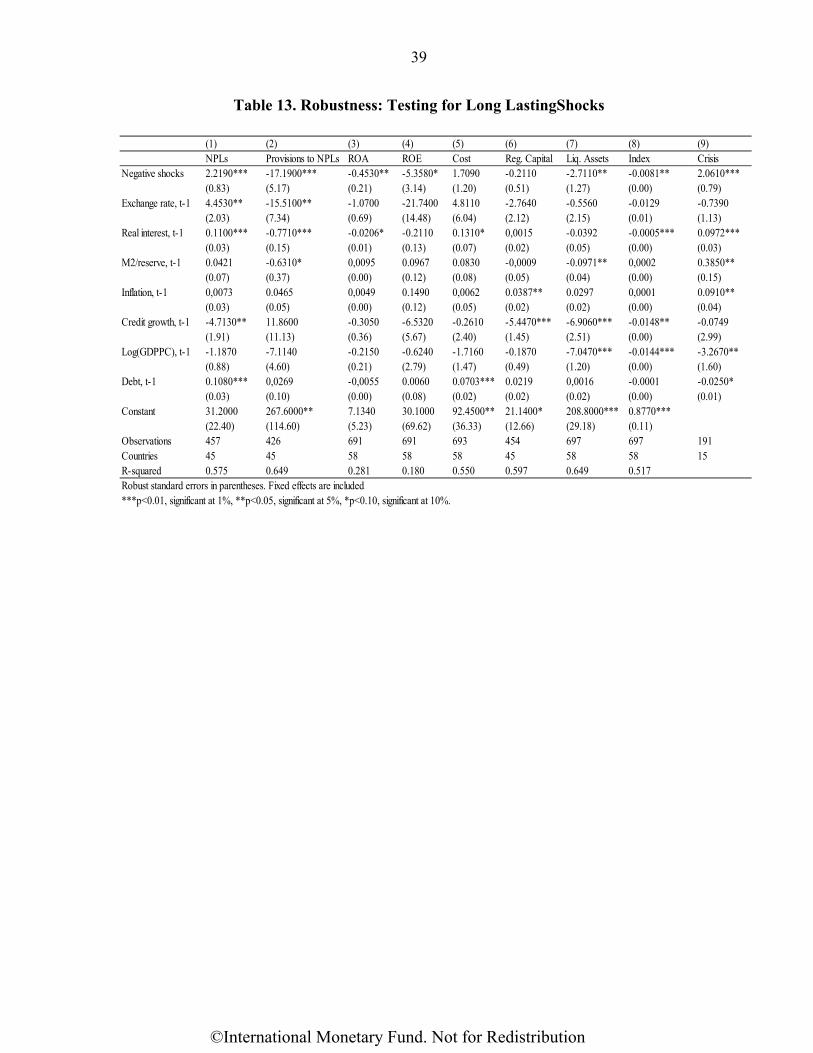
39

Table 13. Robustness: Testing for Long LastingShocks


Negative shocks 2.2190*** -17.1900*** -0.4530** -5.3580* 1.7090 -0.2110 -2.7110** -0.0081** 2.0610***(0.83) (5.17) (0.21) (3.14) (1.20) (0.51) (1.27) (0.00) (0.79)

Exchange rate, t-1 4.4530** -15.5100** -1.0700 -21.7400 4.8110 -2.7640 -0.5560 -0.0129 -0.7390(2.03) (7.34) (0.69) (14.48) (6.04) (2.12) (2.15) (0.01) (1.13)

Real interest, t-1 0.1100*** -0.7710*** -0.0206* -0.2110 0.1310* 0,0015 -0.0392 -0.0005*** 0.0972***(0.03) (0.15) (0.01) (0.13) (0.07) (0.02) (0.05) (0.00) (0.03)

M2/reserve, t-1 0.0421 -0.6310* 0,0095 0.0967 0.0830 -0,0009 -0.0971** 0,0002 0.3850**(0.07) (0.37) (0.00) (0.12) (0.08) (0.05) (0.04) (0.00) (0.15)

Inflation, t-1 0,0073 0.0465 0,0049 0.1490 0,0062 0.0387** 0.0297 0,0001 0.0910**(0.03) (0.05) (0.00) (0.12) (0.05) (0.02) (0.02) (0.00) (0.04)

Credit growth, t-1 -4.7130** 11.8600 -0.3050 -6.5320 -0.2610 -5.4470*** -6.9060*** -0.0148** -0.0749(1.91) (11.13) (0.36) (5.67) (2.40) (1.45) (2.51) (0.00) (2.99)

Log(GDPPC), t-1 -1.1870 -7.1140 -0.2150 -0.6240 -1.7160 -0.1870 -7.0470*** -0.0144*** -3.2670**(0.88) (4.60) (0.21) (2.79) (1.47) (0.49) (1.20) (0.00) (1.60)

Debt, t-1 0.1080*** 0,0269 -0,0055 0.0060 0.0703*** 0.0219 0,0016 -0.0001 -0.0250*(0.03) (0.10) (0.00) (0.08) (0.02) (0.02) (0.02) (0.00) (0.01)

Constant 31.2000 267.6000** 7.1340 30.1000 92.4500** 21.1400* 208.8000*** 0.8770***(22.40) (114.60) (5.23) (69.62) (36.33) (12.66) (29.18) (0.11)

Observations 457 426 691 691 693 454 697 697 191Countries 45 45 58 58 58 45 58 58 15R-squared 0.575 0.649 0.281 0.180 0.550 0.597 0.649 0.517Robust standard errors in parentheses. Fixed effects are included***p<0.01, significant at 1%, **p<0.05, significant at 5%, *p<0.10, significant at 10%.


40

Table 14. Robustness: Different Extreme Shocks Samples


Negative shocks 2.2840*** -16.0300*** -0.5810*** -6.5350*** 1.5370 -0.3440 -1.9730 -0.0083** 1.8750**(0.65) (3.82) (0.18) (2.52) (1.05) (0.41) (1.21) (0.00) (0.79)

Observations 457 426 691 691 693 454 697 697 191Countries 45 45 58 58 58 45 58 58 15R-squared 0.5800 0.6530 0.2870 0.1830 0.5500 0.5970 0.6480 0.5180

Negative shocks 2.4380*** -16.0500*** -0.5180*** -5.8240* 1.6610 -0.3130 -2.0420* -0.0082** 1.9880**(0.66) (3.789) (0.20) (3.04) (1.07) (0.43) (1.19) (0.00) (0.77)


Negative shocks 2.7950*** -14.9000*** -0.5960*** -6.6700** 1.9430* -0.3660 -1.8120 -0.0075** 2.2620***(0.68) (3.78) (0.21) (3.21) (1.12) (0.45) (1.20) (0.00) (0.77)

Observations 457 426 691 691 693 454 697 697 191Countries 45 45 58 58 58 45 58 58 150.5870 0.587 0.6500 0.2880 0.1830 0.5510 0.5970 0.6480 0.5170

Negative shocks 2.9380*** -15.5300*** -0.6830*** -8.4970** 1.2410 -0.7940* -1.7940 -0.0091** 2.2410***(0.69) (3.86) (0.24) (3.88) (1.09) (0.45) (1.23) (0.00) (0.71)


Negative shocks 3.17200*** -16.4700*** -0.7710*** -9.4360** 0.8990 -0.8040* -1.7210 -0.0122*** 2.0600***(0.69) (3.76) (0.24) (3.98) (1.11) (0.45) (1.22) (0.00) (0.65)


Negative shocks 3.1060*** -15.4700*** -0.8450*** -10.3900** 1.3190 -0.5570 -1.1280 -0.0088** 2.7630***(0.73) (3.97) (0.27) (4.48) (1.16) (0.47) (1.28) (0.00) (0.77)


Negative shocks 3.1290*** -15.2100*** -0.8960*** -11.2400** 0.2000 -0.6480 -0.6870 -0.0090** 3.5970***(0.79) (4.34) (0.31) (5.15) (1.22) (0.52) (1.35) (0.00) (0.93)


Negative shocks 2.7930*** -14.8000*** -0.9450** -11.8300* 0.8370 -0.8460 -0.7470 -0.0112** 3.7410***(0.97) (4.82) (0.40) (6.93) (1.44) (0.63) (1.61) (0.00) (1.15)


Negative shocks 3.3080*** -13.2200*** -0.9310*** -11.4300** 0.3930 -0.8430 -0.4070 -0.0096** 3.4860***(0.83) (4.51) (0.33) (5.62) (1.29) (0.54) (1.43) (0.00) (0.99)


Negative shocks 3.3930*** -14.5300*** -1.1600** -15.3600* 1.0060 -1.3330 -1.2300 -0.0148** 7.4050***(1.16) (4.94) (0.48) (8.48) (1.67) (0.81) (1.79) (0.00) (2.09)

Observations 457 426 691 691 693 454 697 697 191Countries 45 45 58 58 58 45 58 58 15R-squared 0.5820 0.6430 0.2990 0.1950 0.5490 0.6010 0.6470 0.5210Note that all control variables and fixed effects are included. Robust standard errors in parentheses***p<0.01, significant at 1%, **p<0.05, significant at 5%, *p<0.10, significant at 10%.

50% most extreme shocks






All





41

Table 15. Robustness: Instability of Commodity Price Shocks

Table 16. Effects of Positive Shocks

(1) (2) (3) (4) (5) (6) (8) (9)VARIABLES NPLs Provisions to NPLs ROA ROE Cost Reg. Capital Liq. Assets IndexPrice unpredictability 0.0623*** -0.3010* -0.0195*** -0.1930* -0.1780*** -0,0079 0.1000* -0.0005***

(0.01) (0.17) (0.00) (0.09) (0.04) (0.01) (0.05) (0.00)Exchange rate, t-1 3.9560* -9.4330 -0.7800 -19.1600 3.3520 -1.7550 3.2490 -0,0013

(2.17) (9.28) (0.81) (16.94) (7.57) (2.36) (3.88) (0.01)Real interest, t-1 0.0144 0.2920 -0.0063 -0,0681 0.1390* 0.0300 0.1050 0,0001

(0.03) (0.18) (0.01) (0.09) (0.07) (0.02) (0.06) (0.00)M2/reserve, t-1 -0.1120* -0.4970 0,0071 0.1450 -0.0788 -0.1900*** 0.0648 0,0003

(0.06) (0.40) (0.01) (0.13) (0.11) (0.07) (0.13) (0.00)Inflation, t-1 -0.0279 0.1270* 0,0052 0.1540 0.0305 0.0395** 0.0325 0,0001

(0.03) (0.07) (0.01) (0.14) (0.06) (0.02) (0.03) (0.00)Credit growth, t-1 -3.4010* 6.6770 0.4090 0.3370 2.2090 -1.1780 0.1270 0,0083

(1.96) (12.20) (0.37) (5.28) (2.67) (1.66) (2.72) (0.00)Log(GDPPC), t-1 -0.3140* 10.6000*** -0.2550*** -2.2040** -0.0009 -0.9080*** 0.9040 0.0010

(0.18) (1.49) (0.05) (0.86) (0.40) (0.15) (0.56) (0.00)Debt, t-1 0.0701*** 0.0657 -0.0045** -0,0018 0.0664*** -0,0039 0.0861*** 1,00E-04

(0.02) (0.08) (0.00) (0.02) (0.02) (0.01) (0.02) (0.00)Constant 9.8220** -163.6000*** 8.8600*** 75.9500*** 63.7800*** 40.0000*** 3.9820 0.5190***

(4.91) (39.79) (1.44) (22.84) (11.52) (4.19) (15.58) (0.03)Observations 493 462 729 729 731 490 735 735Countries 15 15 15 15 15 15 15 15R-squared 0.3210 0.1760 0.1010 0.0720 0.1290 0.1750 0.0850 0.0890Robust standard errors in parentheses. Fixed effects are included***p<0.01, significant at 1%, **p<0.05, significant at 5%, *p<0.10, significant at 10%.

(1) (2) (3) (4) (5) (6) (7) (8) (9)VARIABLES NPLs Provisions to NPLs ROA ROE Cost Reg. Capital Liq. Assets Index CrisisPositive shocks -9.4360*** 35.6300** 1.5580* 21.6600* -7.8550 -0.9270 4.3700 0.0210 -25.3100*

(2.68) (17.99) (0.83) (12.58) (5.00) (1.46) (5.96) (0.01) (13.99)Exchange rate, t-1 4.8200** -17.3800** -1.0910 -22.0100 4.9340 -2.7800 -0.6610 -0.0132 -0.5780

(1.94) (7.24) (0.70) (14.54) (6.09) (2.12) (2.22) (0.01) (1.17)Real interest, t-1 0.1090*** -0.7990*** -0.0210* -0.2130 0.1310* -4.60e-05 -0.0472 -0.0005*** 0.0864***

(0.03) (0.16) (0.01) (0.13) (0.07) (0.02) (0.05) (0.00) (0.03)M2/reserve, t-1 0.0441 -0.7140** 0,0093 0.0948 0.0828 -0.0037 -0.1010** 0,0002 0.3150**

(0.06) (0.36) (0.01) (0.12) (0.08) (0.05) (0.04) (0.00) (0.15)Inflation, t-1 -0.0014 0.0545 0,0051 0.1500 0,0053 0.0387** 0.0297 0,0001 0.0758**

(0.03) (0.05) (0.01) (0.12) (0.05) (0.02) (0.02) (0.00) (0.04)Credit growth, t-1 -4.4560** 9.6960 -0.3080 -6.5260 -0.2740 -5.4950*** -7.0020*** -0.0150** 0.5590

(1.89) (11.55) (0.37) (5.74) (2.42) (1.45) (2.54) (0.00) (2.94)Log(GDPPC), t-1 -1.8500** -1.4740 -0.1010 0.6430 -2.0920 -0.0789 -6.2510*** -0.0122*** -3.0330**

(0.83) (4.05) (0.22) (2.99) (1.42) (0.48) (1.21) (0.00) (1.50)Debt, t-1 0.1000*** 0.0788 -0.0049 0.0132 0.0680*** 0.0215 0,0034 -3.57e-05 -0.0226*

(0.03) (0.10) (0.00) (0.08) (0.02) (0.02) (0.02) (0.00) (0.01)Constant 48.9500** 120.7000 4.1580 -3.4500 102.5000*** 18.5300 188.7000*** 0.8210***

(21.20) (100.20) (5.35) (75.17) (34.92) (12.51) (29.19) (0.10)Observations 457 426 691 691 693 454 697 697 191Countries 43 43 58 58 58 43 58 58 15R-squared 0.5770 0.6400 0.2790 0.1800 0.5500 0.5970 0.6470 0.5150Robust standard errors in parentheses. Fixed effects are included***p<0.01, significant at 1%, **p<0.05, significant at 5%, *p<0.10, significant at 10%.


42

APPENDICES

Table A1: Sample

Country Commodities Country CommoditiesAngola Petroleum Kyrgyz Republic GoldUnited Arab Emirates Petroleum Kuwait PetroleumArgentina Gas, iron, petroleum Libya PetroleumArmenia Copper, iron Sri Lanka CopperAzerbaijan Petroleum Morocco PhosphateBurundi Gold Mexico PetroleumBulgaria Copper, iron, Petroleum Macedonia. FYR IronBahrain Petroleum Mali GoldBosnia and Herzegovina Aluminium Mongolia Coal, goldBelarus Petroleum Mozambique Aluminum, gasBolivia Gas, gold, petroleum, silver, tin Malaysia Gas, petroleumBotswana Nickel Namibia Copper, zincBrazil Aluminum, gold, iron Niger GoldChile Copper Nigeria PetroleumCote d'Ivoire Petroleum Nicaragua GoldCameroon Aluminum, petroleum Oman Gas, petroleumCongo Republic Petroleum Peru Copper, gold, tinColombia Gas, petroleum Philippines CopperDominican Republic Gold, iron, petroleum Qatar Gas, petroleumAlgeria Gas, petroleum Russian Federation Gas, petroleumEcuador Petroleum Saudi Arabia Gas, petroleumEgypt. Arab Rep. Gas, petroleum Sudan Gold, petroleumEthiopia Gold Syrian Arab Republic PetroleumFiji Gold Togo PhosphateGabon Manganese, petroleum Trinidad and Tobago Gas, petroleumGeorgia Gold, iron Tanzania Gold, silverGhana Gold Uganda GoldGuinea Gold Ukraine IronEquatorial Guinea Petroleum Venezuela. RB Aluminum, iron, petroleumGuyana Gold Vietnam PetroleumIndonesia Coal, copper, gas Yemen. Rep. PetroleumIran. Islamic Rep. Gas, petroleum South Africa Aluminum, coal, gold, ironIraq Petroleum Zambia CopperJordan Phosphate Zimbabwe Gold, iron, nickelKazakhstan Coal, copper, gas, iron, petroleum


43

DEFINITIONS OF EACH INDICATOR ARE AS FOLLOWS:

Banks non-performing loans to gross loans: bank nonperforming loans to total gross loans are the value of nonperforming loans divided by the total value of the loan portfolio (including nonperforming loans before the deduction of specific loan-loss provisions). Provisions to non-performing loans: they show the extent to which non-performing loans are already covered by provisions. A non-performing loan is a loan that is in default or close to being in default. Return on equity: Banks’ after-tax net income to yearly averaged equity. Return on asset: Banks’ after-tax net income to yearly averaged assets. Regulatory capital/risk weighted assets: it is the capital adequacy of deposit takers. It is a ratio of total regulatory capital to its assets held, weighted according to risk of those assets. Liquid assets/short-term funding: the ratio of the value of liquid assets (easily converted to cash) to short-term funding plus total deposits. Liquid assets include cash and due from banks, trading securities and at fair value through income, loans and advances to banks, reverse repos and cash collaterals. Deposits and short term funding includes total customer deposits (current, savings and term) and short term borrowing (money market instruments, CDs and other deposits). Bank cost to income ratio: Operating expenses of a bank as a share of sum of net-interest revenue and other operating income. -Leaven and Valencia (2013): They define banking crisis if two conditions are met:

(i) Significant signs of financial distress in the banking system (as indicated by significant bank runs, losses in the banking system, and/or bank liquidations)

(ii) Significant banking policy intervention measures in response to significant losses in the banking system.

They consider the first year that both criteria are met to be the year when the crisis became systemic. Policy interventions in the banking sector are considered as significant if at least three out of the following six measures have been used:

1) Extensive liquidity support (5 percent of deposits and liabilities to nonresidents)

2) Bank restructuring gross costs (at least 3 percent of GDP)

3) Significant bank nationalizations

4) Significant guarantees put in place

5) Significant asset purchases (at least 5 percent of GDP)

6) Deposit freezes and/or bank holidays.


44

Table A2: Descriptive statistics of the main variables

Variable Obs Mean Std. Dev. Min Max

Price shocks 1,255 0.45 0.41 0 1

NPLs 914 8.61 7.92 0,50 74,10

Provisions to NPLs 843 79.78 45.80 0,83 457,20

ROA 1,825 1.54 2.44 -51,31 20,81

ROE 1,822 12,90 33.52 -732,93 170,95

Cost 1,848 58.41 17.90 8,66 194,53

Reg. capital 918 16.84 5.41 -20,10 48,60

Liq. Assets 1,859 37.37 19.97 4,93 149,29

Index 1,870 0.517 0.06 0.08 0.85

Crisis 2,109 0.03 0.19 0 1


45

Table A3: Data Sources

Code Variable Data sourcesNPLs Non-performing loans IMF FSI databaseProvisions to NPLS Provisions to non-performing loans IMF FSI databaseROA Return on assets IMF FSI databaseROE Return on equity IMF FSI databaseCost Cost-to-income ratio IMF FSI databaseReg. capital Regulatory capital to risk-weighted assets IMF FSI databaseLiq. assets Liquid assets to deposits and short-term funding IMF FSI databaseIndex Composite index of the 7 above variables. Authors’ calculations

CrisisBanking crisis. It is a dummy variable that takes the value of 1 if there is a banking crisis and 0 otherwise.

Laeven and Valencia (2013)

Price shocksDummy variable that takes the value of one if there is a negative price shock and 0 otherwise.

Authors’ calculations

GDP growth Rate of real GDP growth World Economic Outlook (WEO), 2015

Debt Public debt in percentage of GDPAbbas, A.S., N. Belhocine, A. Elganainy and M. Horton (2010). A historical public debt database. IMF Working Paper, 10/245.

Exchange rate Real exchange rate. World Economic Outlook (WEO), 2015

Real interest rateReal interest rate which is equal to nominal interest rate divided by GDP deflator

World Economic Outlook (WEO), 2015

M2/reserves Broad money (M2) to international reserves ratio World Economic Outlook (WEO), 2015Inflation Inflation rate World Economic Outlook (WEO), 2015Credit growth Rate of domestic credit growth World Economic Outlook (WEO), 2015GDPPC GDP per capita World Economic Outlook (WEO), 2015

IMFDummy variable that takes a value of 1 if the country has an IMF program and 0 otherwise.

IMF datasets

Revenue Government revenue in percentage of GDP IMF databaseDeficit Budget balance in percentage of GDP World Economic Outlook (WEO), 2015Debt in foreign cur. Debt in foreign currency over GDP World Economic Outlook (WEO), 2015Unemployment Unemployment rate International Labor Organization database, 2015Savings Domestic savings in percentage of GDP World Economic Outlook (WEO), 2015

SWFSovereign wealth fund. Dummy variable that takes a value of 1 if the country has a SWF in the current year and 0 otherwise.

Peterson Institute for International Economics and IMF survey

Exchange regime Exchange rate regime classification (coarse). Ilzetzki, Reinhart and Rogoff (2008)Private credit Domestic credit to the private sector over GDP World Economic Outlook (WEO), 2015

Polity 2Degree of democracy. The polity 2 score ranges from -10 to +10, with higher value representing more democracy.

Polity IV project (Marshall and Jaggers 2002)

Investment profile It evaluates the risk to investment. High score points equates to very low risk. International Country Risk Guide (ICRG)

CorruptionIt represents the extent to which public power is exercised for private gain, including petty and grand forms of corruption.

Worldwide Governance Indicators - World Bank

Gov. EffectivenessIt measures the quality of public services, the quality of the civil service and the degree of its independence from political pressures and the quality of policy formulation


Reg. QualityIt measures the ability of the government to formulate and implement sound policies and regulations that permit and promote private sector development.


Macro-prudential policies Year-to-year change in the number of macro-prudential instruments Cerutti, Claessens and Laeven (2015)Diversification Extensive diversification of exports IMF datasets


46

References

Abbas, S.M.A., N. Belhocine, A.A. Elganainy, and M. Horton, 2010, “A Historical Public Debt Database”, IMF Working Paper No. 10/245 (Washington: International Monetary Fund).

Alesina, A., F.R. Campante, and G. Tabellini, 2008, Why is Fiscal Policy Often Pro-cyclical? Journal of the European Economic Association, 6(5), 1006-36.

Andersen, E.B., 1970, “Asymptotic Properties of Conditional Maximum-Likelihood Estimators.” Journal of the Royal Statistical Society, 32, 283–301.

Arezki, R., and K. Ismail, 2013, “Boom-bust Cycle, Asymmetrical Fiscal Response and the Dutch Disease”. Journal of Development Economics, 101, 256-267.

Arezki, R., and M. Brückner, 2012, "Commodity Windfalls, Democracy and External Debt," Economic Journal, Royal Economic Society, Vol. 122 (561), pp. 848-866.

Babihuga, R., 2007, “Macroeconomic and Financial Soundness Indicators: An Empirical Investigation,” IMF Working Paper. 07/115 (Washington: International Monetary Fund).

Beck, T., A. Demirguc-Kunt, and R. Levine, 2005, “Bank Concentration and Fragility: Impact and Mechanics”. NBER Working Paper No. 11500.

Bems, R., and I. de Carvalho Filho, 2011, “The Current Account and Precautionary Savings for Exporters of Exhaustible Resources,” Journal of International Economics, Vol. 84.1, pp. 48-64.

Blanchard, O. J., and J. Gali, 2010, “The Macroeconomic Effects of Oil Price Shocks: Why Are the 2000s so Different from the 1970s?” University of Chicago Press. ISBN: 0-226-27886-7

Brückner, M. and A. Ciccone, 2010, “International Commodity Prices, Growth and the Outbreak of Civil War in Sub-Saharan Africa,” The Economic Journal, 120 (544), 519-534.

Caprio, J. and D. Klingebiel, 1999, "Episodes of Systemic and Borderline Financial Crises," World Bank Dataset, January.

Cerutti, E., S. Claessens, and L. Laeven, 2015, “The Use and Effectiveness of Macroprudential Policies: New Evidence”. IMF Working Paper 15/61 (Washington: International Monetary Fund).

Chamberlain, G., 1980, “Analysis of Covariance with Qualitative Data.” Review of Economic Studies, 47, 225– 238.


47

Cherif, R., and F. Hasanov, 2012, “Oil Exporters’ Dilemma: How Much to Save and How Much to Invest”. IMF Working Paper 12/4 (Washington: International Monetary Fund).

Čihák, M., and K. Schaeck, 2007, “How Well do Aggregate Bank Ratios Identify Banking Problems?” IMF Working Paper 07/275 (Washington: International Monetary Fund).

Combes, J-L., C.H. Ebeke, S.M.N. Etoudi, and T.U. Yogo, 2014, “Are Remittances and Foreign Aid a Hedge Against Food Price Shocks in Developing Countries?” World Development, 54, 81-98.

Deaton, A. 1999, “Commodity Prices and Growth in Africa.” Journal of Economic Perspectives 13 (3): 23-40.

Deaton, A., and R. Miller 1995, International Commodity Prices, Macroeconomic Performance, and Politics in Sub-Saharan Africa. Princeton, NJ: Princeton Studies in International Finance, No 79.

De Bock, R., and A. Demyanets, 2012, “Bank Asset Quality in Emerging Markets: Determinants and Spillovers”. IMF Working Paper 12/71 (Washington: International Monetary Fund).

Dehn, J., 2000, “Commodity Price Uncertainty and Shocks: Implications for Economic Growth”. Centre for the study of African Economics. University of Oxford. WPS/2000-10.

Demirgüç-Kunt, A., and E. Detragiache, 2000, “Monitoring Banking Sector Fragility: a Multivariate Logit Approach”. World Bank Economic Review, 14 (2), 287–307.

Demirgüç-Kunt, A., and E. Detragiache, 2005, “Cross-country Empirical Studies of Systemic Bank Distress: A survey”. IMF Working Paper 05/96 (Washington: International Monetary Fund).

Egbo, O.P., 2012, “Universal Basis of Bank Failure—The Nigeria Case” Developing Country Studies, 2(10).

Eichengreen, B., and A. Rose, 1998, “Staying Afloat When the Wind Shifts: External Factors and Emerging-Market Banking Crises,” NBER Working Paper No. 6370 (Cambridge, Massachusetts: National Bureau of Economic Research).

Francis, M., 2003, “Governance and Financial Fragility: Evidence from a Cross-Section of Countries.” Bank of Canada Working Paper No. 2003-34.

Ha, V.T.V., L.V. Trien, and H. Diep, 2014, “Macro Determinants on Non-performing Loans and Stress Testing of Vietnamese Commercial Banks’ Credit Risk”. Journal of Science: Economics and Business, Vol. 30, No. 5E (2014) 1-16.


48

International Monetary Fund, 2011, “Macroprudential Policy: An Organizing Framework,” https://www.imf.org/external/np/pp/eng/2011/031411.pdf

Ilzetzki, Ethan O., Carmen M. Reinhart and Kenneth S. Rogoff, 2008, “Exchange Rate Arrangements into the 21st Century: Will the Anchor Currency Hold?” mimeo (University of Maryland and Harvard University).

Kaminsky, G., and C. M. Reinhart, 1999, “The Twin Crises: The Causes of Banking and Balance of Payments Problems,” American Economic Review, 89, 473–500.

Klein, N. 2013, “Non-Performing Loans in CESEE: Determinants and Impact on Macroeconomic Performance”. IMF Working Paper 13/72 (Washington: International Monetary Fund).

Laeven, L., and F.V. Valencia, 2013, “Systemic Banking Crisis Database: an Update”. IMF Economic Review, 61, 225–270.

Lledó, V., I. Yackovlev, and L. Gadenne, 2009, “Cyclical Patterns of Government Expenditures in Sub-Saharan Africa: Facts and Factors”. IMF Working Paper 09/274 (Washington: International Monetary Fund).

Makri, V., A. Tsagkanos, and A. Bellas, 2014, “Determinants of Non-Performing Loans: The Case of Eurozone” PANOECONOMICUS, 2, pp. 193-206

Mundell, R., 1961, “A Theory of Optimum Currency Areas,” American Economic Review, 51, 717–25.

Musayev, V., 2014, “Commodity Price Shocks, Conflict and Growth: The Role of Institutional Quality and Political Violence,” MPRA Paper No. 59786.

Sahay, R., M. Čihák, P. N’Diaye, A. Barajas, R. Bi, D. Ayala, Y. Gao, A. Kyobe, L. Nguyen, C. Saborowski, K. Svirydzenka, and S.Reza Yousefi, 2015, “Rethinking Financial Deepening: Stability and Growth in Emerging Markets”, IMF Staff Discussion Note 15/08 (Washington: International Monetary Fund).

Villafuerte, M. and P. Lopez-Murphy, 2010, “Fiscal Policy in Oil Producing Countries During the Recent Oil Price Cycle”. IMF Working Paper 10/28 (Washington: International Monetary Fund).


https://www.imf.org/external/np/pp/eng/2011/031411.pdf

wp/16/12 - imf elibrary

Documents