world energy projection system plus: commercial module...u.s. energy information administration |...

World Energy Projection System Plus:

Commercial Module

August 2016

Independent Statistics & Analysis

www.eia.gov

U.S. Department of Energy

Washington, DC 20585

U.S. Energy Information Administration | World Energy Projection System Plus: Commercial Module i

This report was prepared by the U.S. Energy Information Administration (EIA), the statistical and

analytical agency within the U.S. Department of Energy. By law, EIA’s data, analyses, and forecasts are

independent of approval by any other officer or employee of the United States Government. The views

in this report therefore should not be construed as representing those of the U.S. Department of Energy

or other federal agencies.

August 2016

U.S. Energy Information Administration | World Energy Projection System Plus: Commercial Module 1

Contents

1. Introduction ............................................................................................................................................. 4

Purpose of this report .............................................................................................................................. 4

Model summary ....................................................................................................................................... 4

Model archival citation ............................................................................................................................ 5

Model contact .......................................................................................................................................... 5

Organization of this report ...................................................................................................................... 5

2. Model Purpose ......................................................................................................................................... 6

Model objectives ..................................................................................................................................... 6

Model inputs and outputs ....................................................................................................................... 6

Relationship to other models .................................................................................................................. 8

3. Model Rationale ..................................................................................................................................... 11

Theoretical approach ............................................................................................................................. 11

Model assumptions ............................................................................................................................... 11

4. Model Structure ..................................................................................................................................... 12

Structural overview................................................................................................................................ 12

Flow diagrams ........................................................................................................................................ 13

Key computations .................................................................................................................................. 15

Projection equations .............................................................................................................................. 16

Appendix A. Model Abstract ...................................................................................................................... 23

Model name: ................................................................................................................................... 23

Model acronym: .............................................................................................................................. 23

Model description: .......................................................................................................................... 23

Model purpose: ............................................................................................................................... 23

Most recent model update: ............................................................................................................ 23

Part of another model: .................................................................................................................... 23

Model interfaces: ............................................................................................................................ 23

Official model representative: ........................................................................................................ 23

Documentation: .............................................................................................................................. 24

Archive information: ....................................................................................................................... 24

Energy system described:................................................................................................................ 24

August 2016


Coverage: ........................................................................................................................................ 24

Modeling features: .......................................................................................................................... 24

DOE input sources: .......................................................................................................................... 24

Non-DOE input sources: .................................................................................................................. 24

Independent expert reviews: .......................................................................................................... 24

Computing Environment: ................................................................................................................ 24

Appendix B. Input Data and Variable Descriptions .................................................................................... 25

Appendix C. References ............................................................................................................................. 33

Appendix D. Data Quality ........................................................................................................................... 34

Introduction ........................................................................................................................................... 34

Source and quality of input data ........................................................................................................... 34

August 2016


Tables

Table 1.Regional Coverage of the World Energy Projection System Plus Model ......................................... 6

Table 2. WEPS+ Models that Provide Inputs to the Commercial Model ..................................................... 7

Table 3. Major Exogenous Commercial Model Input Data Series ............................................................... 7

Table 4. Commercial Model Outputs and the WEPS+ Models that Use Them ............................................ 8

Table 5. Commercial Model Projection Equation Coefficients .................................................................. 29

Figures

Figure 1. World Energy Projection System Plus (WEPS+) Model Sequence ................................................ 9

Figure 2. The Commercial Model Relationship to Other WEPS+ Models .................................................. 10

Figure 3. Flowchart for the Commercial Model ......................................................................................... 13

Figure 4. Flowchart for the Comm Subroutine .......................................................................................... 14

Figure 5. Flowchart for the ClnXML Subroutine ......................................................................................... 15

Figure 6. WEPS+ Commercial Model Basic Flows ...................................................................................... 17

August 2016


1. Introduction

Purpose of this report The Commercial Model of the World Energy Projection System Plus (WEPS+) is an energy demand

modeling system of the world commercial end-use sector at a regional level. This report describes the

version of the Commercial Model that was used to produce the commercial sector projections published

in the International Energy Outlook 2016 (IEO2016). The Commercial Model is one of 13 components of

the WEPS+ system. The WEPS+ is a modular system, consisting of a number of separate energy models

that are communicate and work with each other through an integrated system model. The model

components are each developed independently, but are designed with well-defined protocols for

system communication and interactivity. The WEPS+ modeling system uses a shared database (the

“restart” file) that allows all the models to communicate with each other when they are run in sequence

over a number of iterations. The overall WEPS+ system uses an iterative solution technique that forces

convergence of consumption and supply pressures to solve for an equilibrium price.

This report documents the objectives, analytical approach and development of the WEPS+ Commercial

Model. It also catalogues and describes critical assumptions, computational methodology, parameter

estimation techniques, and model source code. This document serves three purposes. First, it is a

reference document providing a detailed description for model analysts, users, and the public. Second, it

meets the legal requirement of the Energy Information Administration (EIA) to provide adequate

documentation in support of its models (Public Law 93-275, section 57.b.1). Third, it facilitates continuity

in model development by providing documentation from which energy analysts can undertake and

analyze their own model enhancements, data updates, and parameter refinements for future projects.

Model summary The WEPS+ Commercial Model for the IEO2016 projects energy consumed by businesses, institutions,

and service organizations. Commercial sector energy use covers a broad range of activities and services

and includes energy used in schools, stores, correctional institutions, restaurants, hotels, hospitals,

museums, office buildings, banks, and sports arenas. Most commercial energy use occurs in buildings or

structures, supplying services such as space heating, water heating, lighting, cooking, and cooling.

Energy consumed for services not associated with buildings, such as for traffic lights and city water and

sewer services, is also categorized as commercial energy use.

The Commercial Model projects commercial consumption for 11 energy sources in each of the 16

WEPS+ regions on an annual basis over a projection period. The model primarily uses a dynamic

econometric equation for the key energy sources, basing the projection on assumptions about future

growth in gross domestic product (GDP), commercial retail energy prices for nine fuels, and a trend

factor. The dynamic equation uses a lagged dependent variable to imperfectly represent stock

accumulation. The GDP and price projections are available to the Commercial Model from the WEPS+

Macroeconomic Model and the supply models through the restart file, which is shared by all WEPS+

models. The trend factor is meant to represent continuing impacts on energy use not directly

represented in GDP and price, and may include a variety of behavioral, structural, and policy-induced

August 2016


activities. The consumption projections generated by the Commercial Model are in turn put into the

restart file for use by other models.

Model archival citation This documentation refers to the WEPS+ Commercial Model, as archived for the International Energy

Outlook 2016 (IEO2016).

Model contact David Peterson

U.S. Energy Information Administration


1000 Independence Avenue, SW

Washington, D.C. 20585

Telephone: (202) 586-5084

E-mail: [email protected]

Organization of this report Chapter 2 of this report discusses the purpose of the Commercial Model, the objectives and the

analytical issues it addresses, the general types of activities and relationships it embodies, the primary

input and output variables, and the relationship of the model to the other models in the WEPS+ system.

Chapter 3 of the report describes the rationale behind the Commercial Model design, providing insights

into further assumption utilized in the model. Chapter 4 describes the model structure in more detail,

including flowcharts, variables, and equations.

mailto:[email protected]

August 2016


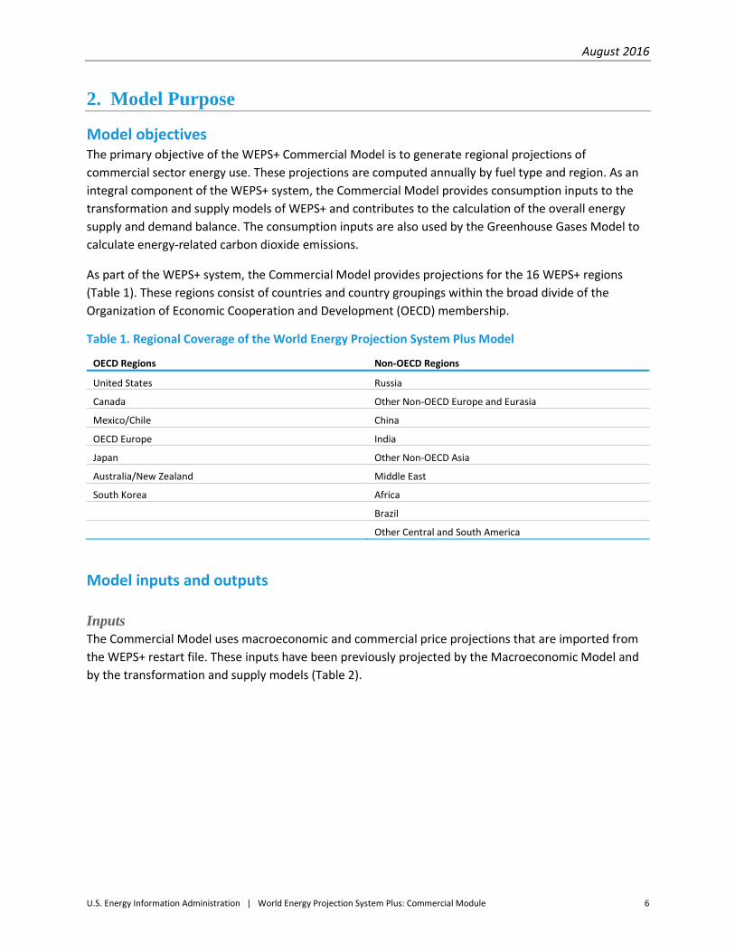
2. Model Purpose

Model objectives The primary objective of the WEPS+ Commercial Model is to generate regional projections of

commercial sector energy use. These projections are computed annually by fuel type and region. As an

integral component of the WEPS+ system, the Commercial Model provides consumption inputs to the

transformation and supply models of WEPS+ and contributes to the calculation of the overall energy

supply and demand balance. The consumption inputs are also used by the Greenhouse Gases Model to

calculate energy-related carbon dioxide emissions.

As part of the WEPS+ system, the Commercial Model provides projections for the 16 WEPS+ regions

(Table 1). These regions consist of countries and country groupings within the broad divide of the

Organization of Economic Cooperation and Development (OECD) membership.

Table 1. Regional Coverage of the World Energy Projection System Plus Model

OECD Regions Non-OECD Regions

United States Russia

Canada Other Non-OECD Europe and Eurasia

Mexico/Chile China

OECD Europe India

Japan Other Non-OECD Asia

Australia/New Zealand Middle East

South Korea Africa

Brazil

Other Central and South America

Model inputs and outputs Inputs

The Commercial Model uses macroeconomic and commercial price projections that are imported from

the WEPS+ restart file. These inputs have been previously projected by the Macroeconomic Model and

by the transformation and supply models (Table 2).

August 2016


Table 2. WEPS+ Models that Provide Inputs to the Commercial Model

Commercial Model Input Source

Gross domestic product Macroeconomic Model

Commercial motor gasoline retail price Refinery Model

Commercial distillate retail price Refinery Model

Commercial residual retail price Refinery Model

Commercial kerosene retail price Refinery Model

Commercial LPG retail price Refinery Model

Commercial natural gas retail price Natural Gas Model

Commercial coal retail price Coal Model

Commercial electricity retail price Electricity Model

Commercial district heat retail price District Heat Model

A number of exogenous data series are also imported into the Commercial Model from the

ComInput.xml file (Table 3).

Table 3. Major Exogenous Commercial Model Input Data Series

Source Input File Model Input

ComInput.xml

GDP elasticities by fuel and region

GDP lag coefficients by region and fuel

Regional by-fuel price elasticities

Regional by-fuel lag coefficients

Regional by-fuel growth trend factors

User adjustment factors (not currently used)

Regional by-fuel multiplicative factors applied to GDP and

price elasticities (currently not used)

Total liquids consumption (hard-wired into input file from

Reference case run; only used in High Oil Price case)

Increment of additional liquids that must be allocated to

natural gas, coal, and electricity (only used in High Oil Price

case)

Outputs

The Commercial Model projects energy consumption in the commercial or service sector by fuel and

region (excluding transportation energy use). Upon completion of a model run, these values are

exported into the WEPS+ restart file for use by other models (Table 4).

August 2016


Table 4. Commercial Model Outputs and the WEPS+ Models that Use Them

Commercial Model Output Destination

Motor gasoline consumption Petroleum Model and Refinery Model

Distillate consumption Petroleum Model and Refinery Model

Residual fuel consumption Petroleum Model and Refinery Model

Kerosene consumption Petroleum Model and Refinery Model

LPG consumption Petroleum Model and Refinery Model

Natural gas consumption Natural Gas Model

Coal consumption Coal Model

Electricity consumption Electricity Model

Heat consumption District Heat Model

Biomass consumption (Placeholder)

Solar consumption (Placeholder)

Relationship to other models The Commercial Model is an integral component of the WEPS+ system, and depends upon other models

in the system for some of its key inputs. In turn, the Commercial Model provides projections of

commercial energy consumption, which are key inputs to other models in the system (Figure 1). A

summary description of the models, flows, and mechanics of the WEPS+ system used for the IEO2016

report is available in a separate Overview documentation.

Through the system, the Commercial Model receives GDP projections from the Macroeconomic Model,

and receives a variety of Commercial retail price projections from various supply and transformation

models (Figure 2). In turn, the Commercial Model provides consumption projections through the system

back to the various supply models.

Although the Commercial Model is an integral part of the WEPS+ system, it can also be easily run as a

standalone, outside of the system. To do that, the Commercial Model would input macroeconomic and

price projections from the WEPS+ system “restart” file as created in a previous system run.

August 2016


Figure 1. World Energy Projection System Plus (WEPS+) Model Sequence

Preprocessor

Start

Macroeconomic

Residential

Commercial

Industrial

Transportation

Electricity

GenerationDistrict Heating

Petroleum

Natural Gas

Coal

Refinery

(Part 2)

Greenhouse

Gases

Main

Postprocessors

(Reports)

Finish

Not Converged

Converged

Transformation Models

Demand ModelsSupply Models

Refinery

(Part 1)

August 2016


Figure 2. The Commercial Model Relationship to Other WEPS+ Models

Commercial

Model

Refinery Model

-Motor gasoline consumption

-Distillate consumption

-Residual consumption

-Kerosene consumption

-LPG consumption

-Commercial motor gasoline retail price

-Commercial distillate retail price

-Commercial residual retail price

-Commercial kerosene retail price

-Commercial LPG retail price

-GDP

Natural Gas Model-Natural gas

consumption

-Commercial natural

gas retail price

Macroeconomic Model Coal Model

World Electricity

Model

-Commercial electricity

retail price

-Electricity

consumption

-Coal consumption

-Commercial coal retail price

District Heat Model

-Heat consumption

-Commercial

district heat

retail price

ComInput.xmlPetroleum Model

-Motor gasoline consumption

-Distillate consumption

-Residual consumption

-Kerosene consumption

-LPG consumption

August 2016


3. Model Rationale

Theoretical approach The Commercial Model makes projections of commercial sector energy consumption based on changes

in GDP, energy prices, and a trend factor. Commercial energy consumption is assumed to follow an

overall trend while increasing with GDP and responding inversely to price changes. Thus the model

projects energy consumption by applying a trend factor and a series of exponential ratio adjustments to

the most recent historical estimates. The exponents of the ratio adjustments, which are imported from

other modeling systems, may be interpreted as elasticity estimates: they represent the extent to which

energy consumption changes in response to changes in GDP and price. Special adjustments are applied

to simulate energy source substitution in the “High World Oil Price” case. Finally, we calibrate the

projections to force consistency with EIA’s short term energy projections.

Model assumptions The Commercial Model makes projections of:

Commercial sector energy consumption, based upon the assumption that changes in consumption are related to changes in GDP

Commercial sector energy prices, based upon an elasticity measure and the dynamics of a stock-adjustment represented by a lagged dependent variable

The projections are also based upon assumptions about autonomous trends representing behavioral,

structural, and/or policy-induced activities. More specifics and the values of the elasticities and trends

are presented in the model structure section below.

August 2016


4. Model Structure

Structural overview The main purpose of the Commercial Model is to estimate annual commercial sector energy

consumption by region and fuel type. The Commercial energy consumption calculations are based on

regional estimates of GDP, commercial fuel prices (by type), and adjustment trend factors.

Consumption is estimated for each of the 16 WEPS+ regions for 11 energy sources: motor gasoline,

distillate fuel, residual fuel, kerosene, liquefied petroleum gas (LPG), natural gas, coal, electricity, heat,

biomass, and solar energy.

The basic structure of the Commercial Model is illustrated in Figure 3. A call from the WEPS+ interface to

the Commercial Model initiates importation of the supporting information from the restart file needed

to complete the projection calculations. The Commercial Model then executes the Comm subroutine,

the major component of the model, which performs all model computations. Finally, the model

executes a subroutine that exports all projections to the restart file for use by other WEPS+ models.

When the Comm subroutine (Figure 4) is initiated by a call from the main Commercial Model, it initiates

a call of the CInXML subroutine (Figure 5), which imports from the ComInput.xml file several exogenous

data series that the model requires. ComInput.xml includes:

The economic (GDP) and price elasticities and lag regression coefficients associated with

regions, fuels, and years. The economic elasticities indicate the extent to which commercial

energy consumption changes in response to changes in GDP.

Multiplicative and shape and elasticity adjustment factors that are associated with each region

and projection year and used if a user-specified adjustment based upon expert judgment is to

be incorporated into the projection

After importing these data, the CInXML subroutine recalculates the GDP and price elasticity factors and

incorporates any shape-and-elasticity adjustment factors. The adjustment factors were not used for

IEO2016 model runs.

The Comm subroutine then begins to compute commercial sector energy consumption projections by

fuel. First, it computes GDP and commercial sector price and trend indices across the projection period

by region and fuel. Next, it calculates an overall commercial sector quantity index as the product of the

GDP, price, and trend indices. If the user has specified additional adjustments, the Comm subroutine

calculates an adjustment index and recalculates the overall commercial sector quantity index to

incorporate the adjustment. It then calculates projections of commercial sector energy consumption by

fuel, region, and year, both with and without any user-specified multiplicative factors.

When a High Oil Price case is being implemented, the Comm subroutine imports two additional data

series from the ComInput.xml file: total liquids consumption by region and year from the Reference

case projections, and a factor that indicates the portion of liquids that will be allocated to natural gas,

coal, and electricity. These amounts are then calculated and allocated to the total commercial sector

natural gas, coal, and electricity projections. Finally, the subroutine calculates commercial sector liquids

August 2016


consumption by region and benchmarks the projections to regional Short-Term Energy Outlook. The

Comm subroutine generates several output files are generated and returns them to the main

Commercial Model routine.

After the Comm subroutine has executed, the WriteRestart subroutine writes the projections to the

restart file for use in future iterations of WEPS+, notably in the refinery model. These output data series

include projections of regional commercial energy use by fuel.

Flow diagrams

Figure 3. Flowchart for the Commercial Model

Start

Main

Routine

Call ReadRestart

Return

Call Comm

Call WriteRestart

August 2016


Figure 4. Flowchart for the Comm Subroutine

Loop by fuel, region, and STEO year

Start

call main model

Call CInXMLComInput.xml

Compute GDP and

residential price and trend

indices

Calculate adjustment index

Loop by fuel, region, and year

Restart file

data

Loop by region,

year, and fuel

Loop by region, year, and fuel

Compute overall

commercial quantity index

User

Adjustment?

Y

N

ComInput.xml

Re-compute commercial

energy consumption with

any multiplicative factors

Recalculate overall commercial

quantity index with adjustment

index


Loop by region, year, and fuelCompute commercial

energy consumption

Y

N


HWOP

Case?

Loop by region, year, and fuel

Allocate difference between

HWOP case and Reference case

commercial petroleum use to

natural gas, coal, and electricity

Benchmark to STEO (using petroleum product consumption

only)

Return

August 2016


Figure 5. Flowchart for the ClnXML Subroutine

Key computations The Commercial Model projects energy that is consumed by businesses, institutions, and service

organizations. Most commercial energy use occurs in buildings or structures, supplying services such as

space heating, water heating, lighting, cooking, and cooling. Energy consumed for services not

associated with buildings, such as for traffic lights and city water and sewer services, is also categorized

as commercial energy use. The model projects commercial sector energy consumption for a number of

energy sources in each of the 16 WEPS+ regions over the projection horizon. The Commercial Model

projects energy consumption for 11 energy sources:

Motor gasoline

Distillate fuel

Residual fuel

Kerosene

LPG

Natural gas

Coal

Electricity

District Heat (steam or hot water)

Start

call Comm

routine

Return

ComInput.xml

Loop by region and fuelImport GDP and price

elasticities and lag

coefficients

Import shape adjustment

values

Loop by region and year

Import multiplicative factors

Loop by region, fuel,

and projection year

Import elasticity adjustment

factors


Recalculate GDP and price

elasticities by applying

adjustment factors


August 2016


Biomass

Solar

The Commercial Model begins by importing the historical data from the WEPS+ shared restart file.

Compiled from the International Energy Agency’s OECD and Non-OECD Statistics and Balances

databases, these data cover detailed energy end-use consumption in the commercial sector. The data

are calibrated to be consistent with the more aggregated energy consumption data from the Energy

Information Administration’s International Statistics Database. These data are processed prior to the

execution of the Commercial Model and are stored in the restart file to provide a common starting point

for all WEPS+ models. The Commercial Model uses the historical data for all years up to the most recent

year available for each of the 16 regions and 11 energy sources.

Macroeconomic and price projections are also imported into the Commercial Model from the restart

file. These data series are projected in previous system iterations by the Macroeconomic Model and by

various transformation and supply models (see Table 2).

Projection equations Figure 6 is a flowchart of the Commercial Model’s major computations, which we discuss in detail here.

The Commercial Model primarily uses econometric assumptions to estimate change in commercial

energy consumption from the year of the most recent historical data (2008). It bases projections for the

key energy sources on a GDP projection, commercial retail energy price projections (for 11 energy

sources—no prices are used for solar or biomass), and a trend factor. The dynamic equation uses a

lagged dependent variable to (imperfectly) represent accumulation of commercial stock—e.g.,

appliances, lighting, and heating and cooling equipment. The Commercial Model obtains the GDP

projections from the WEPS+ Macroeconomic Model through the shared restart file. The GDP projections

are expressed in terms of purchasing power parity in real 2005 dollars. Through the restart file, the

WEPS+ supply models provide by-fuel price projections to the Commercial Model. The prices are all in

terms of real 2009 dollars per million Btu. The trend term is meant to represent continuing impacts on

energy use not directly influenced by GDP and/or price; it may account for the effects of a variety of

behavioral, structural, and policy-induced activities.

August 2016


Figure 6. WEPS+ Commercial Model Basic Flows

The variables used in the projection equations are all expressed in terms of indices indicating change

relative to the most recent available historical value. The indexing approach allows the model to

consider only changes in the GDP and prices, not their actual levels. The effects of the three drivers of

the projection—GDP, prices, and the trend term—are each estimated separately and then multiplied

together to get an overall index reflecting projected change in commercial energy consumption. The

overall index is then applied to the most recent historical consumption value to compute the projection.

GDP index equation

For each region r and projection year y, we first compute the ratio of the GDP in year y to the GDP in the

most recent historical data year, LHYr (both adjusted to reflect purchasing power parity):

𝐺𝐷𝑃𝐼(𝑟, 𝑦) = 𝐺𝐷𝑃_𝑃𝑃𝑃(𝑟, 𝑦)

𝐺𝐷𝑃_𝑃𝑃𝑃(𝑟, 𝑦 = 𝐿𝐻𝑌𝑟)

The index for the GDP-influenced part of the projection for fuel f and region r in year y is then given by

𝐺𝐷𝑃𝐼𝑑𝑥(𝑓, 𝑟, 𝑦) = exp (𝐺𝐷𝑃𝐸𝑙𝑎𝑠(𝑓, 𝑟) ∗ ln(𝐺𝐷𝑃𝐼(𝑟, 𝑦)) + 𝐺𝐷𝑃𝐿𝑎𝑔(𝑓, 𝑟) ∗ ln(𝐺𝐷𝑃𝐼𝑑𝑥(𝑓, 𝑟, 𝑦 − 1)))

Calculate GDP index using elasticity and lag coefficients

Calculate price index using elasticity and lag coefficients

Implement trend index

Calculate overall commercial sector energy demand index

using GDP and price indices and trend index

Make exogenous adjustments as necessary

Use index and initial historical data to make consumption

projections by energy source and region

Calibrate liquids consumption to STEO in near term

August 2016


Where: 𝐺𝐷𝑃𝐸𝑙𝑎𝑠(𝑓, 𝑟) and 𝐺𝐷𝑃𝐿𝑎𝑔(𝑓, 𝑟) are exogenous coefficients (read from an input file)

for the GDP and for the lag term, respectively, for fuel 𝑓 in region 𝑟.

The elasticity coefficient, GDPElas(f,r), reflects the extent to which commercial energy consumption

increases (or decreases) with GDP. The index GDPIdx(f,r,y) starts with a value of 1.0 in the last historical

year of 2008.

Price index equation

The effect of prices on commercial energy consumption is estimated in similar fashion, except that the

price change ratio is estimated separately for each fuel. Let

𝐶𝑃𝐼𝑑𝑥(𝑓, 𝑟, 𝑦) = 𝑅𝑒𝑡𝑎𝑖𝑙𝑃𝑟𝑖𝑐𝑒(𝑓, 𝑟, 𝑦)

𝑅𝑒𝑡𝑎𝑖𝑙𝑃𝑟𝑖𝑐𝑒(𝑓, 𝑟, 𝑦 = 𝐿𝐻𝑌𝑟),

Where: 𝑅𝑒𝑡𝑎𝑖𝑙𝑃𝑟𝑖𝑐𝑒(𝑓, 𝑟, 𝑦) is the retail price of fuel 𝑓 in year 𝑦.

Because the oil price spike of 2008 is an outlier to the general price trend, the RetailPrice in 2008 is set

equal to the average of the RetailPrices in 2007 and 2009.

The effect of prices on commercial energy consumption is then estimated as

𝑃𝑟𝑐𝐼𝑑𝑥(𝑓, 𝑟, 𝑦) = exp(𝑃𝑟𝑐𝐸𝑙𝑎𝑠(𝑓, 𝑟) ∗ ln(𝐶𝑃𝐼𝑑𝑥(𝑓, 𝑟, 𝑦)) + 𝑃𝑅𝐶𝐿𝑎𝑔(𝑓, 𝑟) ∗ ln(𝑃𝑟𝑐𝐼𝑑𝑥(𝑓, 𝑟, 𝑦 − 1))),

Where: PrcElas(f,r) and PrcLag(f,r) are exogenous coefficients (read from an input file) for the

price ratio and the lag term, respectively. The elasticity coefficient, PrcElas(f,r), reflects

the extent to which commercial consumption of fuel f in region r changes in response to

changes in price.

Prices are available for all primary nonrenewable fuels (i.e., all except electricity, district heat, solar, and

biomass).

Trend index

The trend coefficient, TrendGR(f,r), which is read from an input file, represents a constant as an annual

growth rate applied to consumption projections for all years. The growth rate is used to calculate the

trend index term for the last model year, applying the growth rate over the period from the last

historical year to the last model year. The index begins in 2008 with a value of 1.0. Once the implied

value for 2035 has been calculated, the model fills in all the intervening years by linear interpolation:

𝐸𝑓𝑓𝐼𝑑𝑥(𝑓, 𝑟, 𝑦 = 2035) = 𝐸𝑓𝑓𝐼𝑑𝑥(𝑓, 𝑟, 𝑦 = 2008) ∗ 𝑇𝑟𝑒𝑛𝑑𝐺𝑅(𝑓, 𝑟, 𝑦)(2035−2008)

For years from 2009 to 2034:

𝐸𝑓𝑓𝐼𝑑𝑥(𝑓, 𝑟, 𝑦) = 𝐸𝑓𝑓𝐼𝑑𝑥(𝑓, 𝑟, 𝑦 = 2008) + (𝐸𝑓𝑓𝐼𝑑𝑥(𝑓, 𝑟, 𝑦 = 2035) − 𝐸𝑓𝑓𝐼𝑑𝑥(𝑓, 𝑟, 𝑦 = 2008)

(𝑦 − 2008)(2035 − 2008)⁄

August 2016


Overall projection index

The overall projection index for each region and fuel is calculated by multiplying by the GDP index, price

index, and efficiency index:

𝐶𝑄𝐼𝑑𝑥(𝑓, 𝑟, 𝑦) = 𝐺𝐷𝑃𝐼𝑑𝑥(𝑓, 𝑟, 𝑦) ∗ 𝑃𝑟𝑑𝐼𝑑𝑥(𝑓, 𝑟, 𝑦) ∗ 𝐸𝑓𝑓𝐼𝑑𝑥(𝑓, 𝑟, 𝑦)

Where: 𝐶𝑄𝐼𝑑𝑥 is the overall projection index in each region, for each fuel, over the projection

horizon.

Exogenous inflection algorithm

The model projection described thus far consists of an index based on a GDP projection, a price

projection, and a trend factor. The trend projection is computed by linear interpolation between the

2005 value and a target value for 2030. In some cases, however, linear interpolation may not be

appropriate for the particular projection, because a different structural or behavioral trend is expected.

For example, consumption of a specific fuel in a specific region may have grown rapidly in recent years

and be expected to reach saturation, resulting in a moderation of the trend. The model therefore allows

the user to modify the projection index by adding an exogenous inflection.

To accomplish this, the user specifies the year for the midpoint of the inflection and a fraction indicating

the strength of the inflection. The fraction would be a number such as 1.1, indicating that in the

specified year the projection index should be 1.1 times its original value. A value of 1.0 has no effect and

a value of 0.9 means the projection index in the inflection year should be 0.9 times its original value. The

algorithm then will also modify all the other projection index points to smooth the series on each side of

the inflection point. For example, if the inflection point is at 2010, then the values from 2006 through

2009 are smoothed based up the values in 2005 and 2010, and the values from 2011 through 2029 are

smoothed based up the values in 2010 and 2030. The smoothing algorithm uses a sine wave so that

points close to the inflection point are modified more than the points nearer to the end points of the

series. This approach is meant to approximate a spline smoothing technique without the computational

complexity of the spline calculation.

For the IEO2016 Reference case, exogenous inflection factors were used for adjusting electricity

projections for the following regions and years:

Mexico/Chile in 2015, inflection factor = 1.15

OECD Europe in 2012, inflection factor = 1.10

Australia/New Zealand in 2012, inflection factor = 1.15

China in 2010, inflection factor = 2.35

India in 2010, inflection factor = 1.20

Other Central and South America in 2014, adjustment factor = 1.04

Exogenous inflection factors were also used to adjust the following fuels for the Middle East region:

Motor gasoline in 2010, inflection factor = 1.20

Distillate in 2010, inflection factor = 1.20

Residual in 2010, inflection factor = 1.20

Kerosene in 2010, inflection factor = 1.20

LPG in 2010, inflection factor = 1.20

August 2016


Exogenous inflection factors therefore affect only 11 out of the 176 IEO2016 Reference case series (11

fuels multiplied by 16 regions).

Consumption projection

Finally, the historical starting consumption values are multiplied by the projection indices to project

consumption over the projection horizon for each fuel f, region r, and year y:

𝐶𝑄𝑡𝑦(𝑓, 𝑟, 𝑦) = 𝐶𝑄𝐼𝑑𝑥(𝑓, 𝑟, 𝑦) ∗ 𝐻𝑄𝑡𝑦(𝑓, 𝑟, 𝑦 = 2008)

Where: 𝐶𝑄𝐼𝑑𝑥 is the overall projection index in each region, for each fuel, over the projection

horizon

𝐻𝑄𝑡𝑦 is the historical consumption in 2008 by region and fuel

𝐶𝑄𝑡𝑦 is the resulting consumption projection over the projection horizon by region and

fuel

The above equation is for all of the fuels except biomass and solar. The consumption of biomass and

solar is not part of the equation primarily because there are no prices for solar and biomass, but also

because these fuels account for a small percentage of commercial energy consumption. Very little solar

energy is being used in commercial activities. Although a comparatively large amount of biomass is used

in some regions, much of it is unmarketed and therefore not captured in the EIA’s historical

international energy data.

Adjustment factors

In order to provide user control over the projections, the input file contains factors that users can set to

adjust estimates for any fuel in any region and year. The system simply multiplies the specified

consumption projection value by the user-specified factor. This function is not expected to be widely

used and was not used for the IEO2016.

High World Oil Price fuel substitution

In the High World Oil Price (HWOP) scenario, the level of petroleum consumption declines significantly.

The model formulation shown above, however, assumes no elasticity of substitution across fuels. This

assumption was considered appropriate for the original Reference case, because the model was

“calibrated” through user judgment for each of the individual fuels. However, because high oil prices

may cause considerable substitution away from petroleum-based fuels, a simple algorithm was built into

the model to recognize this fuel substitution.

In the HWOP case, a portion of the decline in petroleum consumption from the level in the Reference

case is replaced by increases in consumption of other fuels. In order to determine how much petroleum

consumption has declined from the Reference case, the system first reads in some data that specify the

level of petroleum consumption in the Reference case. These data are supplemented with other data

that provide the fractional increment of the petroleum that will be replaced by other fuels. In the input

file, the fractional increment is set to be 0.5 in all regions, meaning that 50 percent of the petroleum

decrease in the HWOP case will be replaced by an increase in other fuel substitutions. The model

August 2016


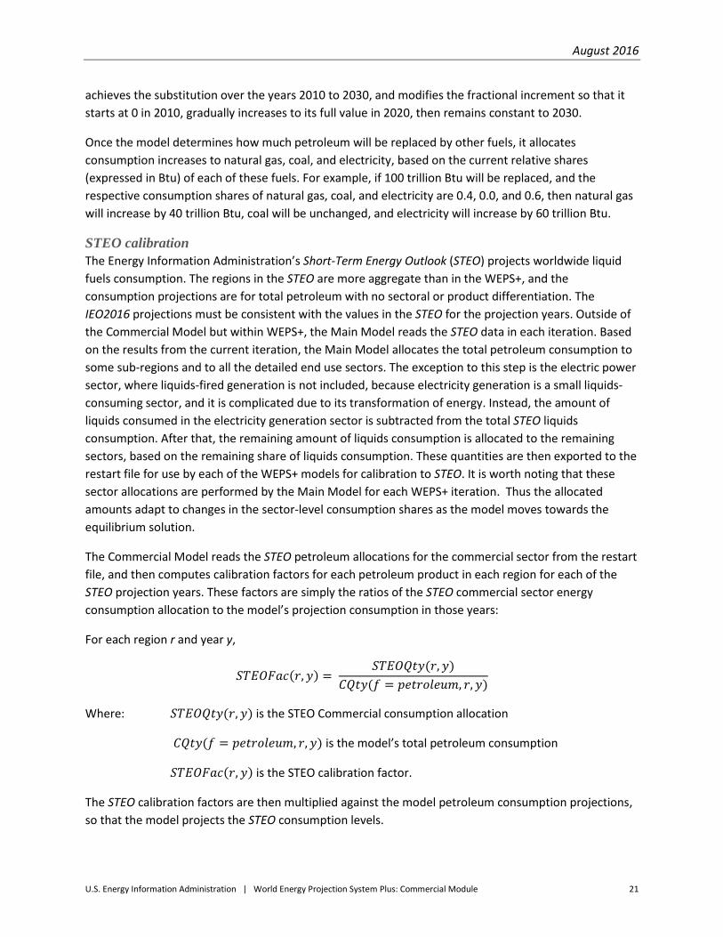
achieves the substitution over the years 2010 to 2030, and modifies the fractional increment so that it

starts at 0 in 2010, gradually increases to its full value in 2020, then remains constant to 2030.

Once the model determines how much petroleum will be replaced by other fuels, it allocates

consumption increases to natural gas, coal, and electricity, based on the current relative shares

(expressed in Btu) of each of these fuels. For example, if 100 trillion Btu will be replaced, and the

respective consumption shares of natural gas, coal, and electricity are 0.4, 0.0, and 0.6, then natural gas

will increase by 40 trillion Btu, coal will be unchanged, and electricity will increase by 60 trillion Btu.

STEO calibration

The Energy Information Administration’s Short-Term Energy Outlook (STEO) projects worldwide liquid

fuels consumption. The regions in the STEO are more aggregate than in the WEPS+, and the

consumption projections are for total petroleum with no sectoral or product differentiation. The

IEO2016 projections must be consistent with the values in the STEO for the projection years. Outside of

the Commercial Model but within WEPS+, the Main Model reads the STEO data in each iteration. Based

on the results from the current iteration, the Main Model allocates the total petroleum consumption to

some sub-regions and to all the detailed end use sectors. The exception to this step is the electric power

sector, where liquids-fired generation is not included, because electricity generation is a small liquids-

consuming sector, and it is complicated due to its transformation of energy. Instead, the amount of

liquids consumed in the electricity generation sector is subtracted from the total STEO liquids

consumption. After that, the remaining amount of liquids consumption is allocated to the remaining

sectors, based on the remaining share of liquids consumption. These quantities are then exported to the

restart file for use by each of the WEPS+ models for calibration to STEO. It is worth noting that these

sector allocations are performed by the Main Model for each WEPS+ iteration. Thus the allocated

amounts adapt to changes in the sector-level consumption shares as the model moves towards the

equilibrium solution.

The Commercial Model reads the STEO petroleum allocations for the commercial sector from the restart

file, and then computes calibration factors for each petroleum product in each region for each of the

STEO projection years. These factors are simply the ratios of the STEO commercial sector energy

consumption allocation to the model’s projection consumption in those years:

For each region r and year y,

𝑆𝑇𝐸𝑂𝐹𝑎𝑐(𝑟, 𝑦) = 𝑆𝑇𝐸𝑂𝑄𝑡𝑦(𝑟, 𝑦)

𝐶𝑄𝑡𝑦(𝑓 = 𝑝𝑒𝑡𝑟𝑜𝑙𝑒𝑢𝑚, 𝑟, 𝑦)

Where: 𝑆𝑇𝐸𝑂𝑄𝑡𝑦(𝑟, 𝑦) is the STEO Commercial consumption allocation

𝐶𝑄𝑡𝑦(𝑓 = 𝑝𝑒𝑡𝑟𝑜𝑙𝑒𝑢𝑚, 𝑟, 𝑦) is the model’s total petroleum consumption

𝑆𝑇𝐸𝑂𝐹𝑎𝑐(𝑟, 𝑦) is the STEO calibration factor.

The STEO calibration factors are then multiplied against the model petroleum consumption projections,

so that the model projects the STEO consumption levels.

August 2016


𝑄𝑀𝐺𝑅𝑆(𝑟, 𝑦) = 𝑄𝑀𝐺𝑅𝑆′(𝑟, 𝑦) ∗ 𝑆𝑇𝐸𝑂𝐹𝑎𝑐(𝑟, 𝑦)

𝑄𝐷𝑆𝑅𝑆(𝑟, 𝑦) = 𝑄𝐷𝑆𝑅𝑆′(𝑟, 𝑦) ∗ 𝑆𝑇𝐸𝑂𝐹𝑎𝑐(𝑟, 𝑦)

𝑄𝑅𝑆𝑅𝑆(𝑟, 𝑦) = 𝑄𝑅𝑆𝑅𝑆′(𝑟, 𝑦) ∗ 𝑆𝑇𝐸𝑂𝐹𝑎𝑐(𝑟, 𝑦)

𝑄𝐾𝑆𝑅𝑆(𝑟, 𝑦) = 𝑄𝐾𝑆𝑅𝑆′(𝑟, 𝑦) ∗ 𝑆𝑇𝐸𝑂𝐹𝑎𝑐(𝑟, 𝑦)

𝑄𝐿𝐺𝑅𝑆(𝑟, 𝑦) = 𝑄𝐿𝐺𝑅𝑆′(𝑟, 𝑦) ∗ 𝑆𝑇𝐸𝑂𝐹𝑎𝑐(𝑟, 𝑦)

Where: 𝑄𝑀𝐺𝑅𝑆 is the commercial motor gasoline consumption

𝑄𝐷𝑆𝑅𝑆 is the commercial distillate consumption

𝑄𝑅𝑆𝑅𝑆 is the commercial residual consumption

𝑄𝐾𝑆𝑅𝑆 is the commercial kerosene consumption

𝑄𝐿𝐺𝑅𝑆 is the commercial LPG consumption

Because the magnitude of STEO calibration adjustment for the last STEO year can be significant, a break

in series could result if the WEPS+ consumption levels for the following were left unadjusted. The STEO

calibration factors are therefore applied, in mitigated form, to the projections for years immediately

after the last STEO year, providing a smooth transition from the STEO-calibrated projections to the

uncalibrated WEPS+ projections.

August 2016


Appendix A. Model Abstract

Model name:

Commercial Model of the World Energy Projection System Plus

Model acronym:

Commercial Model

Model description:

The Commercial Model of the World Energy Projection System Plus (WEPS+) models world commercial

energy demand and provides consumption projections for 11 energy sources in 16 international regions.

For the IEO2016, the Commercial Model provided energy consumption projections for the commercial

or services sector. The 11 energy sources covered include motor gasoline, distillate fuel, residual fuel,

kerosene, liquid petroleum gas, natural gas, coal, electricity, heat, solar, and biomass.

Model purpose:

As a component of the World Energy Projection System Plus (WEPS+) integrated modeling system, the

Commercial Model generates long-term projections of commercial sector energy consumption. The

model also provides consumption inputs for a variety of the other WEPS+ models. The model provides a

tool for analysis of international commercial sector energy use within the WEPS+ system, and can be run

independently as a standalone model.

Most recent model update:

October 2010

Part of another model:

World Energy Projection System Plus (WEPS+)

Model interfaces:

The Commercial Model receives inputs from and provides output to the Macroeconomic Model,

Refinery Model, Natural Gas Model, Coal Model, Electricity Model, and District Heat Model through the

common, shared interface file of the WEPS+ restart file. In addition, the Commercial Model provides

output to the Petroleum Model, again through the common, shared interface file.

Official model representative:

David Peterson

U.S. Energy Information Administration


1000 Independence Avenue, SW

Washington, D.C. 20585

Telephone: (202) 586-5084

E-mail: [email protected]

mailto:[email protected]

August 2016


Documentation:

Energy Information Administration, U.S. Department of Energy, Commercial Model of the World Energy

Projection System Plus: Model Documentation 2011, DOE/EIA-M075(2011) (Washington, DC, August

2011).

Archive information:

The model is archived as part of the World Energy Projection System Plus archive of the runs used to

generate the International Energy Outlook 2016.

Energy system described:

International commercial sector energy consumption.

Coverage:

Geographic: Sixteen WEPS+ regions: U.S., Canada, Mexico/Chile, OECD Europe, Japan, Australia/New Zealand, South Korea, Russia, Other non-OECD Europe and Eurasia, China, India, other non-OECD Asia, Middle East, Africa, Brazil, and other Central and South America.

Mode: total commercial energy consumption.

Time Unit/Frequency: Annual.

Modeling features:

The Commercial Model makes projections of commercial sector energy consumption based upon

changes in GDP, energy prices, and a trend term. The model uses a dynamic simulation approach, using

elasticities to model the changes over time and a lagged dependent variable to simulate dynamic

adjustments.

DOE input sources:

Energy Information Administration, International Energy Statistics Database.

Energy Information Administration, Short Term Energy Outlook (STEO), Washington, D.C.

Non-DOE input sources:

International Energy Agency (IEA), Energy Balances of OECD Countries, Paris, 2010.

International Energy Agency (IEA), Energy Balances of Non-OECD Countries, Paris, 2010.

IHS Global Insight, World Overview, Third Quarter 2010 (Lexington, MA, November 2010).

Independent expert reviews:

None.

Computing Environment:

Hardware/operating system: Basic PC with Windows.

Language/software used: Python, Fortran 90/95

Run Time/Storage: Standalone model with one iteration runs in about 3-4 seconds, CPU memory is

minimal, inputs/executable/outputs require less than 20MB storage.

Special features: None.

August 2016


Appendix B. Input Data and Variable Descriptions

The following variables represent data input from the file ComInput.xml.

Classification: Input variable.

GDPElas(f,r): GDP elasticity by fuel (motor gasoline, distillate, residual, kerosene, LPG, natural

gas, coal, electricity, and heat; excludes renewable energy sources) and region

GDPLag(f,r): GDP lag coefficient by region and fuel

PrcElas(f,r): Regional by-fuel price elasticity

PrcLag(f,r): Regional by fuel price lag coefficient

TrendGR(f,r): Regional growth trend term by fuel

MltFac(f,r,y): Commercial multiplicative factor by region, fuel (motor gasoline, distillate, residual

fuel kerosene, LPG, natural gas, coal, electricity, heat, solar, and biomass) and

projection year

AdjYr(f,r): User adjustment term to change shape of Commercial consumption trend path by

fuel and region (note: not currently used in the model)

EGDPFac(f, r): Regional by-fuel multiplicative factors applied to GDP elasticities (note: currently all

set to 1.0)

EPrcFac(f,r): Regional by-fuel multiplicative factors applied to price elasticities (note: currently

all set to 1.0)

PetRef(r,y): Total liquids consumption in the Reference case by region and year (note: this

must physically be updated to current reference case when user intends to run a

High Oil Price scenario)

PetFacA(r): Increment of additional liquids in the High Oil Price case that must be allocated to

natural gas, coal, and electricity by region

The following variables represent data input from the restart file.

Classification: Input variable from the Macroeconomic Model, Refinery Model, and supply models.

GDP_PPP(r,y): Regional GDP expressed in purchasing power parity by year

PMGCM(r,y): Retail price of motor gasoline for commercial sector energy use by region and year

PDSCM(r,y): Retail price of distillate fuel for commercial sector energy use by region and year

PRSCM(r,y): Retail price of residual fuel for commercial sector energy use by region and year

PKSCM(r,y): Retail price of kerosene for commercial sector energy use by region and year

PLGCM(r,y): Retail price of liquefied petroleum gas for commercial sector energy use by region

and year

August 2016


PNGCM(r,y): Retail price of natural gas for commercial sector energy use by region and year

PCLCM(r,y): Retail price of coal for commercial sector energy use by region and year

PELCM(r,y): Retail price of electricity for commercial sector energy use by region and year

PHTCM(r,y): Retail price of heat for commercial sector energy use by region and year

AMGSCM(r,y): Carbon price increment to the commercial sector motor gasoline price associated

with the carbon allowance price by region and year (dollars per million Btu)

ADSCM(r,y): Carbon price increment to the commercial sector distillate (diesel) fuel price

associated with the carbon allowance price by region and year (dollars per million

Btu)

ARSCM(r,y): Carbon price increment to the commercial sector distillate (diesel) fuel price


Btu)

AKSCM(r,y): Carbon price increment to the commercial sector kerosene price associated with

the carbon allowance price by region and year (dollars per million Btu)

ALGCM(r,y): Carbon price increment to the commercial sector liquefied petroleum gas price


Btu)

ANGCM(r,y): Carbon price increment to the commercial sector natural gas price associated with


ACLCM(r,y): Carbon price increment to the commercial sector coal price associated with the

carbon allowance price by region and year (dollars per million Btu)

AELCM(r,y): Carbon price increment to the commercial sector electricity price associated with


AHTCM(r,y): Carbon price increment to the commercial sector heat price associated with the

carbon allowance price by region and year (dollars per million Btu)

QHMGCM(r,y): Historical motor gasoline consumption in the commercial sector by region and year

QHDSCM(r,y): Historical distillate fuel consumption in the commercial sector by region and year

QHKSCM(r,y): Historical kerosene consumption in the commercial sector by region and year

Convergence complete

QHRSCM(r,y): Historical residual fuel consumption in the commercial sector by region and year

QHLGCM(r,y): Historical liquefied petroleum gas consumption in the commercial sector by region

and year

QHSPCM(r,y): Historical sequestered petroleum fuel consumption in the commercial sector by

region and year

August 2016


QHNGCM(r,y): Historical natural gas consumption in the commercial sector by region and year

QHCLCM(r,y): Historical coal consumption in the commercial sector by region and year

QHELCM(r,y): Historical electricity consumption in the commercial sector by region and year

QHHTCM(r,y): Historical heat consumption in the commercial sector by region and year

QHBMCM(r,y): Historical biomass consumption in the commercial sector by region and year

QHSLCM(r,y): Historical solar energy consumption in the commercial sector by region and year

STEOPTCM(r,y): Projections of liquids for the commercial sector based upon EIA’s Short-Term

Energy Outlook by region and year

The following variables are calculated in the subroutine Comm.

Classification: Computed variable.

XPrc(f,r,y): By-fuel regional price adjusted according to carbon price

CQIdx(f,r,y): Commercial sector overall index combining GDP, price, and trend by fuel, region,

and year

GDPIdx(f,r,y): GDP index by fuel, region, and year

PrcIdx(f,r,y): Price index by fuel, region, and year

EffIdx (f,r,y): Trend term growth index by fuel, region, and year

AdjIdx(f,r,y): Adjustment index to apply a user adjustment term to the consumption curves to

effect a trend change (not currently used in the model)

QMGCM(r,y): Consumption of commercial sector motor gasoline by region and year

QDSCM(r,y): Consumption of commercial sector distillate fuel by region and year

QRSCM(r,y): Consumption of commercial sector residual fuel by region and year

QKSCM(r,y): Consumption of commercial sector kerosene by region and year

QLGCM(r,y): Consumption of commercial sector liquefied petroleum gas by region and year

QNGCM(r,y): Consumption of commercial sector natural gas by region and year

QCLCM(r,y): Consumption of commercial sector coal by region and year

QELCM(r,y): Consumption of commercial sector electricity by region and year

QHTCM(r,y): Consumption of commercial sector district heat by region and year

QBMCM(r,y): Consumption of commercial sector biomass by region and year

QSLCM(r,y): Consumption of commercial sector solar energy by region and year

August 2016


Coefficient sources

The elasticity and the lag coefficients used in the Commercial Model were largely developed from the

U.S. National Energy Modeling System (NEMS) Commercial Module and adapted to the WEPS+

international regions. These elasticities were computed in an Excel spreadsheet through an analysis of

the relationship between a previous Annual Energy Outlook Reference case, the corresponding High and

Low Economic Growth cases, and the corresponding High and Low Oil Price cases. For example, GDP

elasticities were calculated for each year, by sector and fuel, by first examining the difference in energy

demand, relative to the difference in GDP, between the Reference case and the high GDP case. This

comparison process was repeated using the Reference case and the low Economic Growth (i.e., low

GDP) case.

The estimated GDP elasticities varied across scenarios. In general, the average of the High and Low

Economic Growth cases was used in the WEPS+. In some cases, modifications based on analyst

judgment were applied to ensure reasonability.

The price elasticities were calculated in essentially the same manner, using the results of NEMS runs

were for high and low world oil prices. In these runs, prices for the non-petroleum fuels also changed,

and the changes were used for sensitivity analysis. When the price elasticity coefficients were used and

placed into WEPS+, the level of the GDP elasticities were increased by a factor of 1.25 for many of the

developing or rapidly changing regions, including Mexico/Chile, South Korea, and all of the non-OECD

regions.

The Commercial Model coefficients were used in a calibration process to provide a projection for each

energy source based on the previous Commercial Model projections for the IEO. This was accomplished

by calculating a target growth pattern resulting in growth similar to that in previous IEO reports, but

accounting for subsequent GDP and price changes. This is done in an attempt to capture the extent of

future efficiency or usage trends that have been established through accumulated expert judgment and

built into previous projections. This final calibration, based on the trends incorporated in previous

projections and on expert judgment, provides some consistency with previous projections, but is

ultimately validated during the run process with newer and more current information or understanding.

Coefficients used for IEO2016

Table 5 provides the coefficients that were used in the projection equation for the IEO2016. These are

largely determined in the process described above, but in several cases, various coefficients (typically

the trend factor) were changed based on analyst judgment. It is worth noting that in most cases the

elasticities and lag coefficients vary little from region to region (GDP varies somewhat more) and among

the petroleum products.

August 2016


Table 5. Commercial Model Projection Equation Coefficients

GDPElas GDPLag PrcElas PrcLag TrendGR

USA MG 0.083 0.695 -0.136 0.533 -0.0064

USA DS 0.083 0.695 -0.136 0.533 -0.0064

USA RS 0.083 0.695 -0.136 0.533 -0.0064

USA KS 0.083 0.695 -0.136 0.533 -0.0064

USA LG 0.083 0.695 -0.136 0.533 -0.0064

USA NG 0.100 0.819 -0.240 0.032 -0.0002

USA CL 0.100 0.500 -0.100 0.500 -0.0051

USA EL 0.074 0.865 -0.147 0.609 0.0084

USA HT 0.037 0.865 -0.074 0.305 0.0004

CAN MG 0.083 0.695 -0.136 0.533 0.0013

CAN DS 0.083 0.695 -0.136 0.533 0.0013

CAN RS 0.083 0.695 -0.136 0.533 0.0013

CAN KS 0.083 0.695 -0.136 0.533 0.0013

CAN LG 0.083 0.695 -0.136 0.533 0.0013

CAN NG 0.100 0.500 -0.100 0.032 0.0050

CAN CL 0.100 0.500 -0.100 0.500 -0.0036

CAN EL 0.074 0.865 -0.147 0.609 0.0141

CAN HT 0.037 0.865 -0.074 0.305 0.0005

MEX MG 0.104 0.695 -0.136 0.533 0.0039

MEX DS 0.104 0.695 -0.136 0.533 0.0039

MEX RS 0.104 0.695 -0.136 0.533 0.0039

MEX KS 0.104 0.695 -0.136 0.533 0.0039

MEX LG 0.104 0.695 -0.136 0.533 0.0039

MEX NG 0.125 0.819 -0.240 0.032 0.0160

MEX CL 0.125 0.500 -0.100 0.500 -0.0082

MEX EL 0.093 0.865 -0.147 0.609 0.0353

MEX HT 0.046 0.865 -0.074 0.305 -0.0044

EUR MG 0.083 0.695 -0.136 0.533 -0.0067

EUR DS 0.083 0.695 -0.136 0.533 -0.0067

EUR RS 0.083 0.695 -0.136 0.533 -0.0067

EUR KS 0.083 0.695 -0.136 0.533 -0.0067

EUR LG 0.083 0.695 -0.136 0.533 -0.0067

EUR NG 0.100 0.819 -0.240 0.032 -0.0026

EUR CL 0.100 0.500 -0.100 0.500 -0.0166

EUR EL 0.074 0.865 -0.174 0.609 0.0091

EUR HT 0.037 0.865 -0.074 0.305 0.0007

JPN MG 0.083 0.695 -0.136 0.533 -0.0033

JPN DS 0.083 0.695 -0.136 0.533 -0.0033

August 2016


Table 5. Commercial Model Projection Equation Coefficients (cont.)


JPN RS 0.083 0.695 -0.136 0.533 -0.0033

JPN KS 0.083 0.695 -0.136 0.533 -0.0033

JPN LG 0.083 0.695 -0.136 0.533 -0.0033

JPN NG 0.100 0.819 -0.240 0.032 0.0012

JPN CL 0.100 0.500 -0.100 0.500 -0.0084

JPN EL 0.074 0.865 -0.147 0.609 0.0051

JPN HT 0.037 0.865 -0.074 0.305 0.0031

ANZ MG 0.083 0.695 -0.136 0.533 -0.0022

ANZ DS 0.083 0.695 -0.136 0.533 -0.0022

ANZ RS 0.083 0.695 -0.136 0.533 -0.0022

ANZ KS 0.083 0.695 -0.136 0.533 -0.0022

ANZ LG 0.083 0.695 -0.136 0.533 -0.0022

ANZ NG 0.100 0.819 -0.240 0.032 -0.0073

ANZ CL 0.100 0.500 -0.100 0.500 -0.0075

ANZ EL 0.074 0.865 -0.147 0.609 0.0061

ANZ HT 0.037 0.865 -0.147 0.609 0.0061

SKO MG 0.104 0.695 -0.136 0.533 -0.0074

SKO DS 0.104 0.695 -0.136 0.533 -0.0074

SKO RS 0.104 0.695 -0.136 0.533 -0.0074

SKO KS 0.104 0.695 -0.136 0.533 -0.0074

SKO LG 0.104 0.695 -0.136 0.533 -0.0074

SKO NG 0.125 0.819 -0.240 0.032 0.0021

SKO CL 0.125 0.500 -0.100 0.500 -0.0074

SKO EL 0.093 0.865 -0.147 0.609 0.0087

SKO HT 0.046 0.865 -0.074 0.305 -0.0039

RUS MG 0.104 0.695 -0.136 0.533 -0.0159

RUS DS 0.104 0.695 -0.136 0.533 -0.0159

RUS RS 0.104 0.695 -0.136 0.533 -0.0159

RUS KS 0.104 0.695 -0.136 0.533 -0.0159

RUS LG 0.104 0.695 -0.136 0.533 -0.0159

RUS NG 0.125 0.819 -0.240 0.032 0.0138

RUS CL 0.125 0.500 -0.100 0.500 -0.0142

RUS EL 0.093 0.865 -0.147 0.609 0.0112

RUS HT 0.046 0.865 -0.074 0.305 -0.0052

URA MG 0.104 0.695 -0.136 0.533 -0.0084

URA DS 0.104 0.695 -0.136 0.533 -0.0084

URA RS 0.104 0.695 -0.136 0.533 -0.0084

URA KS 0.104 0.695 -0.136 0.533 -0.0084

August 2016




URA LG 0.104 0.695 -0.136 0.533 -0.0084

URA NG 0.125 0.819 -0.240 0.032 -0.0077

URA CL 0.125 0.500 -0.100 0.500 -0.0077

URA EL 0.093 0.865 -0.147 0.609 0.0097

URA HT 0.046 0.865 -0.074 0.305 0.0073

CHI MG 0.104 0.695 -0.136 0.533 0.0182

CHI DS 0.104 0.695 -0.136 0.533 0.0182

CHI RS 0.104 0.695 -0.136 0.533 0.0182

CHI KS 0.104 0.695 -0.136 0.533 0.0182

CHI LG 0.104 0.695 -0.136 0.533 0.0182

CHI NG 0.125 0.819 -0.240 0.032 0.0293

CHI CL 0.125 0.500 -0.100 0.500 -0.0012

CHI EL 0.093 0.865 -0.074 0.609 0.0290

CHI HT 0.046 0.865 -0.147 0.305 -0.0113

IND MG 0.104 0.695 -0.136 0.533 -0.0158

IND DS 0.104 0.695 -0.136 0.533 -0.0158

IND RS 0.104 0.695 -0.136 0.533 -0.0158

IND KS 0.104 0.695 -0.136 0.533 -0.0158

IND LG 0.104 0.695 -0.136 0.533 -0.0158

IND NG 0.125 0.819 -0.240 0.032 -0.0363

IND CL 0.125 0.500 -0.100 0.500 0.0172

IND EL 0.093 0.865 -0.147 0.609 0.0269

IND HT 0.046 0.865 -0.074 0.305 -0.0099

OAS MG 0.104 0.695 -0.136 0.533 0.0035

OAS DS 0.104 0.695 -0.136 0.533 0.0035

OAS RS 0.104 0.695 -0.136 0.533 0.0035

OAS KS 0.104 0.695 -0.136 0.533 0.0035

OAS LG 0.104 0.695 -0.136 0.533 0.0035

OAS NG 0.125 0.819 -0.240 0.032 0.0027

OAS CL 0.125 0.500 -0.100 0.500 0.0188

OAS EL 0.093 0.865 -0.147 0.609 0.0160

OAS HT 0.046 0.865 -0.074 0.305 -0.0064

MID MG 0.104 0.695 -0.136 0.533 0.0128

MID DS 0.104 0.695 -0.136 0.533 0.0128

MID RS 0.104 0.695 -0.136 0.533 0.0128

MID KS 0.104 0.695 -0.136 0.533 0.0128

MID LG 0.104 0.695 -0.136 0.533 0.0128

MID NG 0.125 0.819 -0.240 0.032 0.0045

August 2016




MID CL 0.125 0.500 -0.100 0.500 -0.0086

MID EL 0.093 0.865 -0.147 0.609 0.0136

MID HT 0.046 0.865 -0.074 0.305 -0.0049

AFR MG 0.104 0.695 -0.136 0.533 0.0076

AFR DS 0.104 0.695 -0.136 0.533 0.0076

AFR RS 0.104 0.695 -0.136 0.533 0.0076

AFR KS 0.104 0.695 -0.136 0.533 0.0076

AFR LG 0.104 0.695 -0.136 0.533 0.0076

AFR NG 0.125 0.819 -0.240 0.032 0.0263

AFR CL 0.125 0.500 -0.100 0.500 0.0130

AFR EL 0.093 0.865 -0.147 0.609 0.0189

AFR HT 0.046 0.865 -0.074 0.305 -0.0189

BRZ MG 0.104 0.695 -0.136 0.533 0.0033

BRZ DS 0.104 0.695 -0.136 0.533 0.0033

BRZ RS 0.104 0.695 -0.136 0.533 0.0033

BRZ KS 0.104 0.695 -0.136 0.533 0.0033

BRZ LG 0.104 0.695 -0.136 0.533 0.0033

BRZ NG 0.125 0.819 -0.240 0.032 0.0343

BRZ CL 0.125 0.500 -0.100 0.500 -0.0075

BRZ EL 0.093 0.865 -0.147 0.609 0.0210

BRZ HT 0.046 0.865 -0.074 0.305 -0.0037

CSA MG 0.104 0.695 -0.136 0.533 0.0054

CSA DS 0.104 0.695 -0.136 0.533 0.0054

CSA RS 0.104 0.695 -0.136 0.533 0.0054

CSA KS 0.104 0.695 -0.136 0.533 0.0054

CSA LG 0.104 0.695 -0.136 0.533 0.0054

CSA NG 0.125 0.819 -0.240 0.032 0.0071

CSA CL 0.125 0.500 -0.100 0.500 -0.0091

CSA EL 0.093 0.865 -0.147 0.609 0.0081

CSA HT 0.046 0.865 -0.074 0.305 -0.0054

August 2016


Appendix C. References

1. Walter Nicholson, Microeconomic Theory: Basic Principles and Extensions (Harcourt College Publishers, Fort Worth: Texas, 1972).

2. Franklin J. Stermole and John M. Stermole, Economic Evaluation and Investment Decision Methods: Eleventh Edition (Investment Evaluations Corporation, Lockwood, CO, 2006).

3. C. Dahl, International Energy Markets: Understanding Pricing, Policies, and Profits (PennWell Books, March 2004).

4. Alpha C. Chiang, Fundamental Methods of Mathematical Economics (McGraw-Hill Book Company, NY: NY, 1967).

5. Wayne L. Winston, Operations Research: Applications and Algorithms (Brooks/Cole—Thomson Learning, Belmont, CA, 2004).

6. Energy Information Administration, Commercial Sector Demand Module of the National Energy Modeling System: Model Documentation 2010, DOE/EIA-0066(2010) (Washington, DC, May 25, 2010).

7. International Energy Agency, Energy Statistics and Balances of OECD Countries, web site www.iea.org (subscription site).

8. International Energy Agency, Energy Prices and Taxes (Paris, France, quarterly: various issues).

9. International Energy Agency, Energy Technology Perspectives: Strategies and Scenarios to 2050, (Paris, France 2008).

10. International Energy Agency, World Energy Outlook 2010 Edition (Paris, France, November 2010).

August 2016


Appendix D. Data Quality

Introduction The WEPS+ Commercial Model develops projections of world commercial sector energy use by fuel

(motor gasoline, distillate fuel, residual fuel, kerosene, liquid petroleum gas, natural gas, coal, electricity,

heat, solar, and biomass) for 16 regions of the world. These projections are based on the data elements

detailed in Appendix B of this report. In Chapter 4: Model Structure, the documentation details

transformations, estimation methodologies, and resulting inputs required to implement the model

algorithms. The quality of the principal sources of input data is discussed in Appendix D. Information

regarding the quality of parameter estimates and user inputs is provided where available.

Source and quality of input data Source of input data

STEO – Short-term liquid fuel consumption data from 2005 to 2012 are provided by region from

EIA’s Short-Term Energy Outlook.

International Energy Statistics Database – The Energy Information Administration provides

historical data on international energy consumption by fuel type.

International Energy Agency – The subscription site www.iea.org provides historical energy

consumption data for the OECD and non-OECD balances, along with statistics by end-use sector,

product, and country. These data are benchmarked to the historical aggregate energy

consumption data provided in the Energy Information Administration’s international statistical

data base.

NEMS –The assumptions about price and economic elasticities are drawn largely from

assumptions underlying the National Energy Modeling System for the United States. Expert

judgment has, in some cases, been used to alter NEMS assumptions based on additional

information about specific international regions in the WEPS+ system.

Data quality verification

As a part of the input and editing procedure, an extensive program of edits and verifications was used,

including:

Checks on world and U.S. commercial sector fuel consumption, retail prices, and elasticities,

based on previous values, responses, and regional and technical knowledge

Consistency checks

Technical edits to detect and correct errors, extreme variability

world energy projection system plus: commercial module...u.s. energy information administration |...

Documents