December 2011

WORKING PAPERCENTRAL BANK OF ICELAND N

o.

56

By

Jósef Sigurdsson

Unemployment Dynamics and Cyclical Fluctuations in the Icelandic Labour Market

Central Bank of Iceland Working Papers are published by the Economics Departments of the Central Bank of Iceland. The views expressed in them are those of their authors and not necessarily the views of the Central Bank of Icleand.

Also available on the Central Bank of Iceland World Wide Web site (http://www.sedlabanki.is)

All rights reserved. May be reproduced or translated provided the source is stated.

ISSN 1028-9445

Unemployment Dynamics and Cyclical Fluctuations

in the Icelandic Labour Market∗

Josef Sigurdsson†

Central Bank of Iceland

December 2011

Abstract

This paper studies business cycle dynamics in the Icelandic labour market with

the focus on two separate but related dimensions. First, which margin for adjustment

of labour input, the extensive margin or the intensive margin, accounts for more

variation in total working hours? It finds that both margins are important. Variation

in employment accounts for 56% of the overall variation in total hours while variation

in hours per worker contributes 44% to variation in total hours. Second, which of the

two unemployment transition rates, the separation rate or the job-finding rate, drives

the observed fluctuations in unemployment, and how do these transition rates move

over the business cycle? The results show that fluctuations in the separation rate

explain 70% of the total variation in the unemployment rate. Both transition rates

are highly cyclical. The procyclical job finding rate moves roughly contemporaneously

with the cycle, while the countercyclical separation rate is found to lead the cycle.

Keywords: Labour adjustment, Unemployment dynamics, Worker flows

JEL Classification: E32, J63, J64

∗I would like to thank Asgeir Danielsson, Bjarni G. Einarsson, Magnus F. Gudmundsson and RannveigSigurdardottir for helpful discussions and comments. I am grateful to the Directorate of Labour, especiallyKarl Sigurdsson, for generously allowing access to their database. All errors and omissions are mine. Theviews expressed do not necessarily reflect those of the Central Bank of Iceland.

†Economics Department, Central Bank of Iceland, Kalkofnsvegur 1, 150 Reykjavik, Iceland, Email:js@cb.is

1 Introduction

Over the business cycle, there are significant fluctuations in the labour market at various

margins. During expansion, firms increase output and their demand for labour input in

response to changes in aggregate demand. In recessions, however, firms’ output decreases

and their demand for labour input falls. The cyclical variations in labour input may be

attributed to firms’ two margins for adjusting labour input: number of hours per worker

and number of workers employed. The former is referred to as the intensive margin and the

latter as the extensive margin. Furthermore, changes in the relative rates at which labour

input is adjusted through the extensive margin drive the dynamics in the unemployment

rate. Even though changes in labour-market conditions are observed on the surface, these

dynamics underneath remain somewhat opaque.

The objective of this paper is to explore and establish key facts about unemployment

dynamics and cyclical fluctuations in the Icelandic labour market. Such facts are of fun-

damental importance, both for macroeconomic modelling and monetary policy. In recent

years, New Keynesian (NK) models have been used to explain business cycle fluctua-

tions. Equipped with New Keynesian features, including nominal rigidities and imperfect

competition, these models have become a popular tool for analysing macroeconomic is-

sues. However, in the benchmark NK model, all adjustment in labour input takes place

along the intensive margin. This means that the model does not incorporate involun-

tary unemployment. Armed with evidence of involuntary unemployment, economists have

incorporated unemployment into NK models by introducing search frictions along the

lines of Mortensen and Pissarides (1994) (see Gertler and Trigari, 2009; Gertler, Sala and

Trigari, 2008; Blanchard and Gali, 2010).1 However, the standard search and matching

model adjustst labour input exclusively along the extensive margin.2 In order to construct

a macroeconomic model that includes labour market dynamics, it is essential to possess

information on (i) how labour input is adjusted over the business cycle and (ii) what drives

unemployment dynamics.

Decomposing the variance in total hours, I find that 45% of the overall variation is

due to variation in hours per worker, while 55% is due to variation in employment. Both

1For a presentation of the building blocks of the search and matching model see Pissarides (2000).2See e.g. Trigari (2006) for a search and matching model with labour adjustment along both margins.

2

the extensive and the intensive margins are therefore important for adjustment of labour

input, the extensive margin being responsible for slightly more of the overall variation.

Furthermore, hours per worker and employment are found to be positively correlated.

This indicates that over the business cycle, firms adjust labour input in the same direction

along both the intensive and the extensive margin. This evidence highlights the importance

of modelling both workers’ decision to participate in the labour market and the choice of

number of working hours in order to give a good approximation of the adjustment processes

in the labour market.

In small open economies such as Iceland, labour supply can vary significantly due to

migration of native and foreign workers. Workers move between countries in a search

for higher wages and better employment opportunities. Recently, international migration

has become a more important factor in determining the evolution of the labour force in

Iceland. I find evidence of cyclical migration patterns for both foreign and native workers;

as unemployment rises, more native workers move from the country and fewer foreign

workers choose to immigrate. As a business cycle indicator, this relationship between

unemployment and migration leads to fluctuations in labour supply. As a result, a labour

market with international migration would be a desirable component in a NK model for

small open economies such as Iceland.

In Section 3 the attention is turned to exploring and estimating the relative impor-

tance of the drivers of unemployment dynamics. Over time, the unemployment rate is

determined by two factors: inflow of workers into the pool of unemployed and outflow

of workers out of unemployment. If more unemployed workers find a job each month

than workers who become unemployed, then the unemployment rate falls, and vice versa.

The flow approach to modelling unemployment dynamics, e.g. Mortensen and Pissarides

(1994) and Pissarides (2000), relates firms’ hiring, a costly and time-consuming process of

opening vacancies and searching for new workers, to unemployed (and employed) workers’

engagement in a time-consuming job search. The search and matching paradigm aims

at capturing these processes, describing unemployment as an equilibrium phenomemon;

because of search frictions, there is always a positive fraction of the labour force that is

unemployed. However, unemployment is not constant and varies substantially over the

business cycle. A key question is whether business cycle dynamics in unemployment are

3

driven by variation in the job finding rate or in the separation rate.

Even though a clear view of unemployment dynamics is crucial for understanding and

predicting changes in unemployment, there is still lack of consensus on the relative impor-

tance of those driving forces. The conventional view, based on Darby, Haltiwanger and

Plant (1985, 1986) and Blanchard and Diamond (1990), was that job separations are more

cyclical than job findings, implying that inflows into unemployment are the driving force

of unemployment dynamics. This view emphasises that in order to understand unem-

ployment dynamics, one must understand the destruction of jobs and workers’ separation

from jobs. However, in recent studies Hall (2005b) and Shimer (2007) find that job separa-

tions in the US are acyclical and mostly constant over the business cycle while job-finding

is strongly procyclical. Contradicting conventional wisdom, this evidence suggests that

unemployment dynamics are driven by variation in the creation of new matches rather

than variation in separations. A substantial literature has addressed this matter since,

using different methodologies and datasets. Fujita and Ramey (2009) find that variation

in the separation rate contributes between 40% and 70% of the overall variation in un-

employment in the US. Furthermore, Elsby, Michaels and Solon (2009) find that during

recessions, countercyclical inflow rates are important for understanding unemployment

dynamics in the US. Using dynamic decomposition, Smith (2011) finds that for the UK

the contribution of the two transition rates varies over the business cycle, and that the

separation rate contributes more to variation in unemployment during recessions. Elsby,

Hobijn and Sahin (2009) provide a decomposition for fourteen OECD countries. They find

that among Anglo-Saxon economies, the variation in inflows into unemployment accounts

for only one-fifth of the overall variation in unemployment, while the relative contribution

of inflows and outflows is almost even for Continental European and Nordic countries.

Following the literature, I derive the two unemployment hazard rates: the job finding

rate and separation rate. I then solve for those transition rates using monthly data on

worker flows from the Directorate of Labour for the period 2000-2010. Building on the

methodology pioneered in Shimer (2007), the total variation in the unemployment rate is

decomposed into variation due to fluctuations in inflows (the separation rate) and variation

due to fluctuations in outflows (the job finding rate). This allows for assessment of the

4

relative importance of the two different state transitions.3 I find that variation in inflows

into unemployment contribute 70% of the overall variation in unemployment. This is found

true both for the whole sample period and when excluding the 2008-2010 recession, which

was characterized by a sudden, rapid and unusually large increase in unemployment.4

Having evaluated the relative importance of the driving forces of unemployment, I assess

the cyclicality of the two transition rates to determine how these driving forces evolve

over the business cycle. Both transition rates are highly cyclical. The job finding rate

is procyclical and moves contemporaneously with the cycle. The job separation rate is,

however, countercyclical and leads the cycle. Furthermore, changes in the separation rate

are found to lead changes in the job finding rate.

2 Cyclical Fluctuation and Labour Adjustment

In an economy with fully flexible wages, evolution of total hours worked would follow the

evolution in the population as all shocks affecting the labour market would be absorbed

through changes in the wage level. In reality, as found in Sigurdardottir and Sigurdsson

(2011), wages are sticky and adjusted infrequently. As a result of rigid wages, total

hours vary significantly over the business cycle, increasing in booms, but decreasing in

recessions. However, what remains unclear is whether a fall in total hours is caused by

employed workers working fewer hours or because more workers becoming unemployed or

exiting the labour force? I now quantitatively evaluate the importance of the adjustment

margins at business cycle frequencies.

2.1 Adjustment of Total Hours

The data used are from Statistics Iceland’s Labour Force Survey (LFS), which has been

executed with quarterly frequency since 2003, but on a semiannual basis between 1991 and

2002. Quarterly series for the period 1991-2002 are obtained by disaggregating the semi-

3Due to data limitations, I am not able to explore movements in and out of unemployment that arealso entries and exits from the labour market. However, in Section 2 I explore the contribution of variationin labour force participation on variation in total hours. I find that participation fluctuates less thanemployment and explains less of the variation in total hours.

4For our sample period, January 2000 to December 2010, registered unemployment was 3.1% on average.In the 2008-2010 recession, registered unemployment peaked at 9.3% in March 2010.

5

-8

-6

-4

-2

0

2

4

6

8

1992 1994 1996 1998 2000 2002 2004 2006 2008 2010

Total hours Employment Hours per worker

Year

Dev

iati

on f

rom

tre

nd

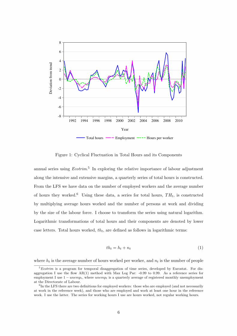
Figure 1: Cyclical Fluctuation in Total Hours and its Components

annual series using Ecotrim.5 In exploring the relative importance of labour adjustment

along the intensive and extensive margins, a quarterly series of total hours is constructed.

From the LFS we have data on the number of employed workers and the average number

of hours they worked.6 Using these data, a series for total hours, THt, is constructed

by multiplying average hours worked and the number of persons at work and dividing

by the size of the labour force. I choose to transform the series using natural logarithm.

Logarithmic transformations of total hours and their components are denoted by lower

case letters. Total hours worked, tht, are defined as follows in logarithmic terms:

tht = ht + nt (1)

where ht is the average number of hours worked per worker, and nt is the number of people

5Ecotrim is a program for temporal disaggregation of time series, developed by Eurostat. For dis-aggregation I use the flow AR(1) method with Max Log Par: -0.99 to 0.99. As a reference series foremployment I use 1− unempt, where unempt is a quarterly average of registered monthly unemploymentat the Directorate of Labour.

6In the LFS there are two definitions for employed workers: those who are employed (and not necessarilyat work in the reference week), and those who are employed and work at least one hour in the referenceweek. I use the latter. The series for working hours I use are hours worked, not regular working hours.

6

Table 1: Business Cycle Variation in Labour Input

Standard deviations of relative deviations from trend

Total hours (th) Hours (h) Employment (n)2.36 1.22 1.47

Correlation

(th, h) (th, n) (n, h)0.84 0.90 0.51

Notes: Data are quarterly time series for the period Q1/1991 - Q3/2011.Total hours, th, are defined as the average hours multiplied by by numberof persons employed and divided by the labour force, and transformedusing natural logarithm. Standard deviations are in percentage terms.

employed in per capita terms, i.e. divided by the size of the labour force. All series are

seasonally adjusted using the Census Bureau’s X12 ARIMA procedure. Since the focus is

on the cyclical fluctuations of hours and employment, the time series are detrended using

Hodrick-Prescott (HP) filter with a standard smoothing parameter for quarterly data.

The series tht, ht and nt are therefore presented as deviations from trend.

Figure 1 plots the cyclical fluctuations in total hours and its components. Total hours

worked fluctuate significantly over the business cycle. The same is true for the two com-

ponents, employment and hours per worker, which both display co-movement with total

hours. During the upswing, 2005-2008, total hours were above trend; both employment

and hours per worker contributed to this deviation. In two contraction periods, 1993-

1994 and 2003, employment was the more important factor, while in 2008-2010, hours per

worker contributed more to the deviation from trend. The fact that adjustment along

the intensive margin is as important as observed highlights the flexibility of the Icelandic

labour market, since the process of hiring new workers is generally time-consuming and

adjustment of labour input through the intensive margin is an efficient channel for re-

sponding to variation in demand.

Table 1 presents standard deviations of total hours, hours per worker, and employ-

ment, as well as correlations between them. The series are deviations from trend.7 Since

7One might be concerned about the variation created by generating quarterly series for the period 1991-2002. I excluded that period and carried out the same analysis. This results in slightly larger standarddeviations and somewhat stronger correlation between the components, especially employment and hours,the correlation coefficient for which is measured at 0.63.

7

the series are in natural logarithms the standard deviations can be interpreted as mean

percentage deviations from trend. The mean deviation in total hours is 2.4 percent, the

deviation in hours per worker is 1.2 percent, and the mean deviation in employment is 1.5

percent. As Figure 1 and Table 1 show, both hours per worker and employment are highly

positively correlated with total hours, the correlation being 0.84 and 0.90 respectively.

Furthermore, the correlation between employment and hours per worker is 0.51. These

results indicate that firms adjust labour input in the same direction over the business

cycle.

In order to obtain a statistical measure of the relative importance of adjustment along

the intensive margin and the extensive margin over the business cycle, a decomposition of

variation in total hours is proposed. The variance of total hours worked, tht, is defined as

follows in terms of the variation in its two components:

var(tht) = var(ht) + var(nt) + 2cov(ht, nt) (2)

Using definitions of variance and covariance, the variation of tht can be written as:

var(tht) = E{(ht + nt − E(ht + nt))(tht − E(tht))}

= E{(ht − E(ht))(tht − E(tht)) + (nt − E(nt))(tht − E(tht))}

= cov(ht, tht) + cov(nt, tht) (3)

The first term on the right-hand-side of (3), cov(ht, tht), is the amount of variation in

tht that is contributed both directly from ht and its correlation with nt. cov(nt, tht) is

similarly the variation in tht that derives from variation in nt and its correlation with ht.

Dividing through equation (3) with var(tht) gives the following:

1 = γh + γn (4)

where γh and γn are given by the following equations:

γh =cov(ht, tht)

var(tht)(5)

8

γn =cov(nt, tht)

var(tht)(6)

Hence, (5) and (6) are the relative contributions of variance in ht and nt to the total

variation in tht. Table 2 reports the values for γh and γn for both the whole sample period

and the subperiod 2003-2011.

Table 2: Decomposition of variance in tht

1991 – 2011 2003 – 2011

Contribution of hours per worker, γh 0.44 0.46Contribution of employment, γn 0.56 0.54

Note: Quarterly time series for the period Q1/1991 - Q4/2002 are generatedby disaggregation of semiannual data using Ecotrim.

I find that both margins of labour adjustment are of almost equal importance. For

the whole sample period, 45% of variation in total hours is due to variation in hours per

worker and 55% due to variation in employment. For the period 2003-2011 the results are

very similar. This evidence indicates that over the business cycle, Icelandic firms adjust

labour input in the same direction both along the intensive and extensive margin, but

not evenly. Furthermore, hours per worker and employment can be interpreted as close

substitutes when firms adjust total hours.

2.2 Labour Force Participation

Variation in the size of the labour force provides another dimension of flexibility in the

labour market. In recessions, firms can adjust labour input by decreasing hours worked

per worker or the number of employed workers. But when workers separate from firms

they do not necessarily enter the pool of unemployed, as they may choose to exit the

labour force. Furthermore, when firms increase labour input by hiring workers, they may

hire workers that were previously outside the labour force. Over the business cycle there

may therefore be a group of workers who enter and exit the labour force depending on the

state of the economy. As a result the size of the labour force, as well as employment and

hours per worker, may move in tandem with the business cycle, providing an additional

9

-8

-6

-4

-2

0

2

4

6

8

1992 1994 1996 1998 2000 2002 2004 2006 2008 2010

Total hours People at work Labour force paricipation

Year

Dev

iati

on f

rom

tre

nd

Figure 2: Cyclical Fluctuation in Labour Force Participation

dimension of labour market flexibility.

Figure 2 plots deviation from trend in total hours, people at work, and labour force

participation. Data are reported on quarterly frequency and scaled with the population

at working age, not the labour force as before. All series are seasonally adjusted using

the X12 ARIMA procedure, transformed using natural logarithms, and detrended using

an HP filter with the conventional smoothing parameter for quarterly data.

As depicted in Figure 2, participation varies over the cycle as people enter and exit the

labour force. However, the variation in the number of people at work is much greater and

co-moves more strongly with total hours. Standard deviations of the relative deviations

from trend are reported in Table 3. The standard deviation of detrended series for people

at work is 1.9 percent, more than twice the standard deviation of the detrended labour

force which has a standard deviation of 0.9 percent. Furthermore, the correlation between

the labour force and total hours is 0.66 which is much weaker than the correlation of either

hours per worker or people at work with total hours. This indicates that the variation in

labour force participation is a secondary factor in explaining cyclical fluctuations in the

labour market.

10

Table 3: Cyclical Fluctuation in the Labour Market

Standard deviations of relative deviations from trend

Total hours (th∗) People at work (ep) Labour Force (lf)2.79 1.89 0.92

Correlation

(th∗, ep) (ep, lf) (th∗, lf)0.93 0.66 0.63

(th∗, h) (ep, h) (lf, h)0.84 0.59 0.43

Notes: Data are quarterly time series for the period Q1/1991 - Q3/2011. Differ-ent from Table 1, total hours, th∗, are defined as the average hours multipliedby by number of persons employed divided by the number of people in work-ing age, and transformed using natural logarithm. Standard deviations are inpercentage terms.

Some of the stylised facts presented here are similar to what studies for other countries

have shown, but others are somewhat different. Similar to the findings in the current

paper are the results in Krause and Lubik (2010) for the U.S., which show that variation

in hours per worker accounts for 33% to 50% of variation in total hours. In an earlier study

on the U.S. labour market, Cho and Cooley (1994) find that only 25% of variation in total

hours can be attributed to variation in hours per worker and the remainder is assigned to

variation of employment. Rogerson and Shimer (2010) conclude that variation in the size

of the labour force is a secondary factor at business cycle frequencies in the U.S., agreeing

with previous evidence in Lilien and Hall (1986). When comparing the U.S. to 17 OECD

countries, Rogerson and Shimer (2010) find that the fraction of people at work is strongly

correlated with total hours in both the U.S. and OECD countries. The correlation is 0.95

in the U.S. and 0.87 on average in the OECD countries. On the other hand they find that

correlation between total hours and hours per worker is strong in the U.S. but weak in

the OECD on average. Moreover, the correlation between the fraction of people at work

and hours per worker is 0.68 in the U.S. but only 0.05 in the OECD on average.8 The

results presented in the current paper indicate that the Icelandic labour market, where

8Rogerson and Shimer (2010) find that in both France and Japan the correlation between total hoursand hours per worker is stronger than the correlation between total hours and employment, unlike in otherOECD countries and the U.S.

11

-1

0

1

2

3

4

1 2 3 4 5 6 7 8

Unemployment rate

Net

mig

rati

on r

ate

- F

ore

ign w

ork

ers

(a) Net migration of foreign workers

-1.2

-1.0

-0.8

-0.6

-0.4

-0.2

0.0

0.2

1 2 3 4 5 6 7 8

Unemployment rate

Net

mig

rati

on r

ate

- Ic

elan

dic

work

ers

(b) Net migration of Icelandic workers

Figure 3: Labour Migration in Iceland: 1991-2010

adjustment takes place along both margins and in the same direction, is more like the

U.S. labour market than the labour markets in other OECD countries. Flexible hours per

worker in Iceland and the U.S. give rise to more flexible labour input than in other OECD

countries since adjustment may in general be thought to be more rigid along the extensive

margin.

2.3 International Migration

In addition to changes in labour force participation, the supply of labour in open economies

adjusts to changes in aggregate demand through migration of workers. During expansion

periods, demand for labour increases and mobile workers in foreign countries may choose

to migrate in order to find employment or higher wages. In a recession, workers may

respond to unemployment or lower purchasing power of wages by migrating. Since labour

migration may be an important margin for labour supply, I end this section by briefly

looking at the cyclicality in labour migration. Figure 3 shows the relationship between

the net migration rate of Icelandic and foreign nationals and unemployment. The rate

is defined as the net number of migrants at working age divided by the labour force.

For foreign nationals, low unemployment, and thus high labour demand, translates into

increasing migration of foreign workers to Iceland.9 Figure 3b shows the relationship

between unemployment and net migration of Icelandic nationals; increased unemployment

9The increase in immigration in 2005-2007 was mainly due to large construction projects domesticallyand a boom that created excess demand for labour in the construction industry, but also due to enlargementof the EU in 2004 that decreased the cost of workers from Central and Eastern Europe in migrating to EUand EEA member states like Iceland.

12

increases emigration. Furthermore, a comparison of Figures 3a and 3b reveals two different

mechanisms that affect labour supply in Iceland. The net migration of Icelandic nationals

is always negative, but it is stronger at times of distressed labour market conditions. Net

migration of foreign nationals, however, is negative when unemployment is above 4%, but

positive when unemployment is lower. Over the last business cycle, the latter mechanism

has become an increasingly important margin for adjustment of labour supply. In the years

2005-2007 – the three observations in the North-West corner of Figure 3a – migration was

especially high, 2.5% of labour force on average. During the recession in 2008-2010, net

migration of foreign workers peaked at 1.3% of the labour force in 2009. Putting these

numbers into perspective, in 2008 foreign nationals were 11% of the labour force.

3 Unemployment Dynamics

In this section, I explore the relative importance of inflows into and outflows out of un-

employment for explaining unemployment dynamics. The methodology used in the paper

follows closely that of Shimer (2007) and Petrongolo and Pissarides (2008), and the dataset

used is administrative data from the Directorate of Labour (DoL). I have information on

the number of both unemployment registrations and deregistrations of claimants at the

DoL in a given month. As the data are biased towards workers who come from employ-

ment, rather than individuals who have been outside the labour force, I follow Petrongolo

and Pissarides (2008) and model unemployment dynamics in an environment where tran-

sition is only between two states: unemployment and employment. Also, it should be

noted that flows in and out of unemployment take place continuously while data on un-

employment flows is discrete. In order to correct for the time-aggregation bias that can

arise due to this fact, I use a method pioneered by Shimer (2007).

3.1 Analytical Framework

Two states are defined for workers in the labour market: employed or unemployed. Time

is denoted with t ∈ {0, 1, 2, ...}, where the interval [t, t + 1) is refered to as period t and

τ ∈ [0, 1] is the time elapsed since beginning of the current time period. Unemployed

workers find job according to a Poisson process, which gives the following probability of

13

finding a job:

P(Ft) = 1− e−ft (7)

where the job finding rate, i.e. the arrival rate of jobs, is ft = − ln(1−P(Ft)). The total

unemployment outflow during period t is then given by:

Γt = (1− e−ft)Ut +

∫ 1

0[1− e−ft(1−τ)]Σt+τ dτ (8)

where Σt+τ is unemployment inflow at t + τ , and Ut is unemployment at the beginning

of period t. Equation (8) is in two parts. The first part of the equation represents the

number of workers who were unemploymed at the beginning of period t but find a new job

during the period. The second part represents the number of workers who were employed

at the beginning of period t, that get separated from their job during the period but find

a new job before the end of period t. The second part of equation (8) therefore accounts

for time aggregation bias following Shimer (2007). In a similar fashion workers separate

from jobs according to a Poisson process. The probability of separation can be written as:

P(St) = 1− e−st (9)

and the separation rate is therefore st = − ln(1−P(St)). The total unemployment inflow

during period t is then:

Σt = (1− e−st)Et +

∫ 1

0[1− e−st(1−τ)]Γt+τ dτ (10)

where Et denotes employment at the beginning of period t and Γt+τ is the unemployment

outflow at time t+τ . Assuming that the unemployment inflows and outflows are uniformly

distributed over the time period t, gives the following expression for total unemployment

outflow:

Γt = (1− e−ft)Ut + (1− 1− e−ft

ft)Σt (11)

and analogously for unemployment inflow:

14

Σt = (1− e−st)Et + (1− 1− e−st

st)Γt (12)

Using monthly data for Γt, Σt, Ut and Et, equations (11) and (12) can be solved for the

continuous-time transition rates ft and st using a conventional numerical solver.

My aim is to examine the cyclical variation in job separation and job finding and to

estimate the contribution of the two flow rates to the variance in unemployment. Denoting

the unemployment rate as ut, the evolution of the unemployment rate can be described in

terms of the continuous-time transition rates:

du

dt≡ ut = (1− ut)st − utft (13)

Equation (13) describes the evolution of unemployment accurately when all inflows into

unemployment are from the pool of employed workers and all flows out of unemployment

are workers who find jobs.10 In steady state the unemployment rate is, by definition,

changing at a rate of zero, ut = 0, which gives:

(1− ut)st = utft (14)

Rearranging the above gives an expression for the flow steady state unemployment:

ut =st

st + ft(15)

This is a key equation of the search and matching model that describe a unique equi-

librium unemployment rate – a flow steady state – in terms of the transition rates ft and

st. If the flow steady state unemployment is a good approximation of the unemployment

rate, a valid decomposition of the unemployment rate can be derived using the job finding

and separation rates. More precisely, the unemployment dynamics can be decomposed

into two components: the variation due to changes in the job finding rate ft, and the

variation due to changes in the job separation rate st. By first-differencing the steady

state unemployment, ∆ut ≡ ut − ut−1, the following expression is obtained:

10Because of data limitations, unemployment can not be described more accurately transitions moreaccurately by taking account to flows in and out of the labour force.

15

∆ut =st

st + ft− st−1

st−1 + ft−1(16)

= (1− ut)ut−1∆stst−1

− (1− ut−1)ut∆ftft−1

Under the approximation ut ≈ ut−1, (16) can be written as a decomposition of the

percentage change in the steady-state unemployment rate:

∆utut−1

= (1− ut)∆stst−1

− (1− ut−1)∆ftft−1

(17)

Elsby et al. (2009) and Fujita and Ramey (2009) use a decomposition in logarithms.

Since ∆utut−1

≈ ∆ln(ut) for small changes, the decomposition (17) can be written in in

logarithmic terms as:

∆ ln ut = (1− ut)∆ ln st︸ ︷︷ ︸Πs

t

−(1− ut−1)∆ ln ft︸ ︷︷ ︸Πf

t

(18)

where Πst and Πt

t are the contribution of changes in the inflow rate and the outflow rate

to the total variation in the unemployment rate, respectively. Equation (18) is a key

equation describing the dynamic evolution of unemployment. Using the decomposition, I

can calculate each components’ contribution to the variance in steady state unemployment

as:

βs =cov(∆ ln ut,Π

st )

var(∆ ln ut)(19)

βf =cov(∆ ln ut,Π

ft )

var(∆ ln ut)(20)

βs and βf represent the relative contribution of the two flow components to the total

variation in unemployment. Therefore, by definition, βs + βf ≈ 1, where any difference

from unity is due to approximation.

16

3.2 The Relative Importance of Ins and Outs

Figure 4 plots monthly worker flow data on unemployment, inflows and outflows for the

period 2000-2010. From month to month there is a considerable variation in all series.

Numerous workers enter and exit the pool of the unemployed each month, causing its

size to vary. However, no clear pattern emerges from the figure. I therefore turn to the

decomposition method presented above to gain a better understanding of the dynamics of

unemployment and its elements.

0

1,000

2,000

3,000

4,000

5,000

0

4,000

8,000

12,000

16,000

20,000

2000 2001 2002 2003 2004 2005 2006 2007 2008 2009 2010

Inflow (left axis) Outflow (left axis) Unemployment (right axis)

Figure 4: Unemployment, Inflow and Outflow

Monthly DoL data for outflow from unemployment (Γt), inflow into unemployment

(Σt), registered unemployment (Ut), and employment (Et), are used to solve equations

(11) and (12) for the continuous-time transition rates ft and st. The series are seasonally

adjusted using the X-12 ARIMA procedure, and quarterly series are generated by averaging

in order to remove excess volatility. The contribution of variation in inflows and outflows

to the overall variation in unemployment, βs and βf , is then calculated using the quarterly

series.

The results for the decomposition of unemployment variance are presented in Table 4.

I find that variation in the inflow rate explains a larger fraction of the overall variation in

the unemployment rate; increased unemployment is driven by increased rate of separation.

For the whole sample period, 2000-2010, changes in the separation rate explain 70% of

the total variation in unemployment. During the recession starting in the autumn of

17

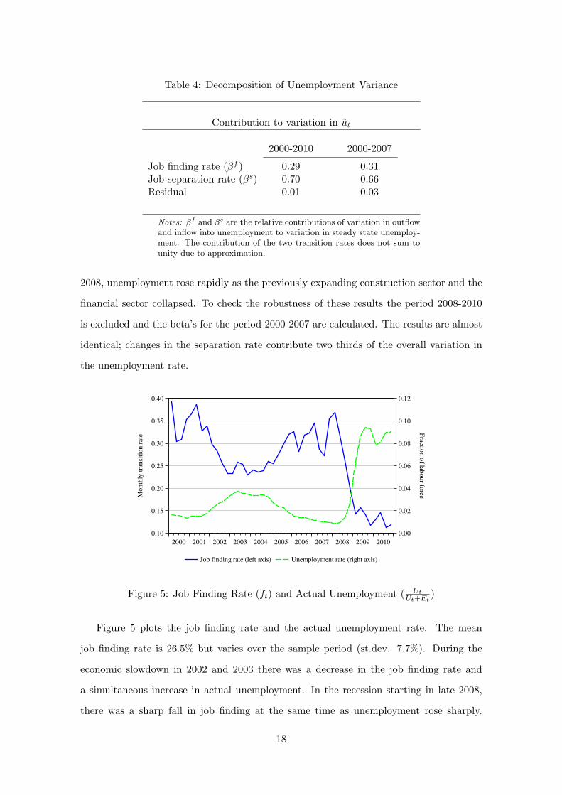
Table 4: Decomposition of Unemployment Variance

Contribution to variation in ut

2000-2010 2000-2007

Job finding rate (βf ) 0.29 0.31Job separation rate (βs) 0.70 0.66Residual 0.01 0.03

Notes: βf and βs are the relative contributions of variation in outflowand inflow into unemployment to variation in steady state unemploy-ment. The contribution of the two transition rates does not sum tounity due to approximation.

2008, unemployment rose rapidly as the previously expanding construction sector and the

financial sector collapsed. To check the robustness of these results the period 2008-2010

is excluded and the beta’s for the period 2000-2007 are calculated. The results are almost

identical; changes in the separation rate contribute two thirds of the overall variation in

the unemployment rate.

0.10

0.15

0.20

0.25

0.30

0.35

0.40

0.00

0.02

0.04

0.06

0.08

0.10

0.12

2000 2001 2002 2003 2004 2005 2006 2007 2008 2009 2010

Job finding rate (left axis) Unemployment rate (right axis)

Mo

nth

ly t

ran

siti

on

rat

eF

raction

of lab

ou

r force

Figure 5: Job Finding Rate (ft) and Actual Unemployment ( UtUt+Et

)

Figure 5 plots the job finding rate and the actual unemployment rate. The mean

job finding rate is 26.5% but varies over the sample period (st.dev. 7.7%). During the

economic slowdown in 2002 and 2003 there was a decrease in the job finding rate and

a simultaneous increase in actual unemployment. In the recession starting in late 2008,

there was a sharp fall in job finding at the same time as unemployment rose sharply.

18

0.000

0.004

0.008

0.012

0.016

0.020

0.024

0.00

0.02

0.04

0.06

0.08

0.10

0.12

2000 2001 2002 2003 2004 2005 2006 2007 2008 2009 2010

Job separation rate (left axis) Unemployment rate (right axis)

Mo

nth

ly t

ran

siti

on

rat

eF

raction

of lab

ou

r force

Figure 6: Job Separation Rate (st) and Actual Unemployment ( UtUt+Et

)

However, as depicted in Figure 6, the separation rate also co-moves strongly with actual

unemployment. The mean monthly separation rate is 0.8%, but it varies substantially

over the period (st.dev. 0.4%). This behaviour of the separation rate during recessions is

somewhat similar to what Elsby, Michaels and Solon (2009) find using U.S. data. They

find that even though outflow from unemployment is the most important driving force

of unemployment variation in the U.S., recessions are characterised with a sudden rise

in the inflow rate at the start of the recession and a parallel increase in unemployment.

Furthermore, they note that in recessions the job separation rate for job leavers falls

while the job separation rate rises for job losers. The evidence presented for the Icelandic

labour market, as the evidence in Elsby, Michaels and Solon (2009), therefore indicates

that increased unemployment in recessions is caused by the destruction of jobs and and

increased number of unemployment spells rather than by a lower job finding rate and

longer unemployment spells.

One of the main assumptions behind the decomposition of unemployment variance is

that the actual unemployment rate is well approximated by the flow steady-state, stst+ft

.

Figure 7 plots the actual unemployment rate from the DoL data and the flow steady state

unemployment rate. It is clear that although the two rates move closely together they

are not identical. The contemporaneous correlation between the two rates is 0.90, but the

correlation peaks at a lag of one quarter at 0.93. As a matter of fact, the unemployment

19

0.00

0.02

0.04

0.06

0.08

0.10

0.12

0.14

2000 2001 2002 2003 2004 2005 2006 2007 2008 2009 2010

Steady-state unemployment Actual unemployment

Fra

ctio

n o

f L

abo

ur

Fo

rce

Figure 7: Steady-state Unemployment ( stst+ft

) and Actual Unemployment ( UtUt+Et

)

rate is moving over time towards flow steady state. This adjustment depends on the

aggregate dynamics of flows in and out of unemployment. By rearranging equation (13)

and dividing on both sides with st + ft, it can be seen that unemployment consistently

trails its flow steady state:

utst + ft

=st

st + ft− ut (21)

= ut − ut

Equation (21) provides valuable insight into the role of turnover dynamics in the labour

market.11 First, it shows that if the steady-state unemployment is above actual unem-

ployment, i.e. the right-hand-side of equation (21) is positive, actual unemployment is

rising, and vice versa. Second, the left-hand-side of equation (21) states that convergence

of unemployment to the flow steady-state is determined by the turnover; the convergence

is faster the more fluid the unemployment dynamics. In other words, as the more frequent

the transitions in and out of unemployment, the closer unemployment is to its flow steady

state.

11The importance of turnover dynamics for unemployment has been discussed in the literature, see Hall(2005a) and Smith (2011). Hall (2005a) argues that turnover dynamics do not play a role in unemploymentdynamics in the U.S. because of high transition rates. Smith (2011) finds that since aggregate transitionsin the U.K. are low, turnover dynamics do matter.

20

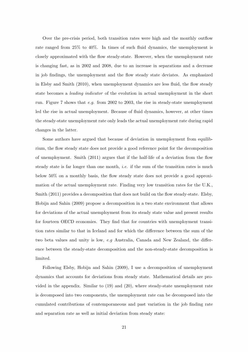
Over the pre-crisis period, both transition rates were high and the monthly outflow

rate ranged from 25% to 40%. In times of such fluid dynamics, the unemployment is

closely approximated with the flow steady-state. However, when the unemployment rate

is changing fast, as in 2002 and 2008, due to an increase in separations and a decrease

in job findings, the unemployment and the flow steady state deviates. As emphasized

in Elsby and Smith (2010), when unemployment dynamics are less fluid, the flow steady

state becomes a leading indicator of the evolution in actual unemployment in the short

run. Figure 7 shows that e.g. from 2002 to 2003, the rise in steady-state unemployment

led the rise in actual unemployment. Because of fluid dynamics, however, at other times

the steady-state unemployment rate only leads the actual unemployment rate during rapid

changes in the latter.

Some authors have argued that because of deviation in unemployment from equilib-

rium, the flow steady state does not provide a good reference point for the decomposition

of unemployment. Smith (2011) argues that if the half-life of a deviation from the flow

steady state is far longer than one month, i.e. if the sum of the transition rates is much

below 50% on a monthly basis, the flow steady state does not provide a good approxi-

mation of the actual unemployment rate. Finding very low transition rates for the U.K.,

Smith (2011) provides a decomposition that does not build on the flow steady-state. Elsby,

Hobijn and Sahin (2009) propose a decomposition in a two state environment that allows

for deviations of the actual unemployment from its steady state value and present results

for fourteen OECD economies. They find that for countries with unemployment transi-

tion rates similar to that in Iceland and for which the difference between the sum of the

two beta values and unity is low, e.g Australia, Canada and New Zealand, the differ-

ence between the steady-state decomposition and the non-steady-state decomposition is

limited.

Following Elsby, Hobijn and Sahin (2009), I use a decomposition of unemployment

dynamics that accounts for deviations from steady state. Mathematical details are pro-

vided in the appendix. Similar to (19) and (20), where steady-state unemployment rate

is decomposed into two components, the unemployment rate can be decomposed into the

cumulated contributions of contemporaneous and past variation in the job finding rate

and separation rate as well as initial deviation from steady state:

21

βs =cov(∆ lnut,Ψ

st )

var(∆ lnut), βf =

cov(∆ lnut,Ψft )

var(∆ lnut), β0 =

cov(∆ lnut,Ψ0t )

var(∆ lnut)

Using this dynamic decomposition I find βs = 0.64 and βf = 0.31, where the difference

of the sum from unity is a residual. These results, which account for deviations of the

unemployment rate from the steady-state, are consistent with the earlier results in the

paper; approximately two-thirds of the overall variation in the unemployment rate is due

to variation in the separation rate and one-third due to variation in the job finding rate.

-1.0

-0.8

-0.5

-0.3

0.0

0.3

0.5

0.8

1.0

-6 -5 -4 -3 -2 -1 0 1 2 3 4 5 6

i =

(a) Correlation between PRODt and ft+i

-1.0

-0.8

-0.5

-0.3

0.0

0.3

0.5

0.8

1.0

-6 -5 -4 -3 -2 -1 0 1 2 3 4 5 6

i =

(b) Correlation between PRODt and st+i

-1.0

-0.8

-0.5

-0.3

0.0

0.3

0.5

0.8

1.0

-6 -5 -4 -3 -2 -1 0 1 2 3 4 5 6

i =

(c) Correlation between ut and ft+i

-1.0

-0.8

-0.5

-0.3

0.0

0.3

0.5

0.8

1.0

-6 -5 -4 -3 -2 -1 0 1 2 3 4 5 6

i =

(d) Correlation between ut and st+i

Figure 8: Cross-Correlograms

4 Inflows and Outflows Over the Business Cycle

Assessment of the relative importance of the two driving forces of unemployment, job find-

ing and separation rates, is essential for understanding unemployment dynamics. However,

in order to understand how unemployment evolves over time it is necessary to study the

22

dynamic co-movement of the transition rates with the business cycle.

I evaluate the dynamic relationships cross-correlating the job finding rate, ft, and

the separation rate, st, with two measures of economic activity (unemployment, ut, and

productivity, PRODt) at various leads and lags.12 The cyclical series are extracted using a

HP filter with a smoothing parameter of 105. The cross-correlations between productivity

and the transition rates are shown in Figures 8a and 8b. For productivity and the job

finding rate the correlation peaks at 0.72 at a lead of one and the cross correlation is

close to being symmetrical around a lead of one. The correlation between productivity

and the separation rate peaks -0.72 but at a lag of three quarters. Figures 8c and 8d

further assess the cyclicality of the transition rates using the unemployment rate as a

measure of economic activity. The results are roughly similar. The correlation between

unemployment and job finding is -0.85 at lags of both one and zero quarters while the

correlation with the separation rate peaks at 0.88 at a lag of two quarters. Figure 9 shows

the cross-correlation between the job finding rate and the separation rate. The transition

rates are highly negatively correlated at lags of zero to three quarters, with the correlation

peaking at -0.78 at lag of one quarter. Changes in the job finding rate are therefore

preceded by changes in the separation rate one period earlier.

-1.0

-0.8

-0.5

-0.3

0.0

0.3

0.5

0.8

1.0

-6 -5 -4 -3 -2 -1 0 1 2 3 4 5 6

i =

Figure 9: Cross-Correlogram of ft and st+i

The evidence presented in Figures 8 and 9 above provides valuable insight into how

unemployment evolves over the business cycle. First, the very strong correlation with

12Productivity, PRODt, is measured as GDP divided by the level of employment in man-years.

23

business cycle indicators implies that unemployment transition rates are highly cyclical.

The job finding rate is highly procyclical and moves contemporaneously with the cycle.

While it too is highly cyclical, the job separation moves inversely to the business cycle

and leads the cycle.

5 Concluding Remarks

The aim of this paper has been to study business cycle dynamics in the Icelandic labour

market and establish facts about adjustment of labour input and the dynamics of un-

employment. I set out to answer two main questions. First, I explored which of the

two adjustment margins, the intensive or the extensive margin, is more important for ad-

justment of labour input in Iceland. According to the results, firms adjust labour input

both by adjusting the number of workers employed and the number of hours worked per

worker. Variation in employment accounts for 56% of the overall variation in total hours

while variation in hours per worker contributes 44%. Furthermore, there is a positive

correlation between employment and hours per worker, indicating that labour input is

adjusted in the same direction along both margins. I find that even though participation

varies over the business cycle, it is a secondary factor in explaining fluctuations in total

hours. I also presented evidence suggesting that international migration is an important

factor for labour supply.

Second, I explored whether the observed variation in unemployment is driven by the

rate at which workers separate from firms or by the rate at which workers find jobs,

and how these transition rates move over the business cycle. According to the evidence

presented, the main driving force of unemployment is variation in the separation rate,

which accounts for 70% of the overall variation in unemployment. Therefore, increased

unemployment during recessions is caused by an increased number of unemployment spells

rather than by longer spells. Both transition rates co-move strongly with the business

cycle. The job finding rate is found to move contemporaneously with the cycle while the

separation rate leads the cycle.

24

References

[1] Blanchard, O. and P. Diamond (1990), “The Cyclical Behaviour of the GrossFlows of U.S. Workers”, Brookings Papers on Economic Activity, vol. 1990(2), pp.85-155.

[2] Blanchard, O. and J. Gali (2010), “Labor Markets and Monetary Policy: ANew Keynesian Model with Unemployment”, American Economic Journal: Macroe-conomics, vol. 2(2), pp. 1-30.

[3] Cho, J. and T.F. Cooley (1994), “Employment and Hours over the Business Cycle”,Journal of Economic Dynamics and Control, vol.18(2), pp.411-432.

[4] Darby, M., J. Haltiwanger and M. Plant (1985), “Unemployment Rate Dynam-ics and Persistent Unemployment under Rational Expectations”, American EconomicReview, vol.75(4), pp.614-637.

[5] Darby, M., J. Haltiwanger and M. Plant (1986), “The Ins and Outs of Unem-ployment: The Ins Win”, NBER Working Paper No. 1997

[6] Elsby, M.W., R. Michaels and G. Solon (2009), “The Ins and Outs of CyclicalUnemployment”, American Economic Journal: Macroeconomics, vol. 1(1), pp. 84-110.

[7] Elsby, M.W., B. Hobijn and A. Sahin (2009), “Unemployment Dynamics in theOECD”, NBER working paper 14617.

[8] Fujita, S. and G. Ramey (2009), “The Cyclicality of Separation and Job FindingRates”, International Economic Review, vol. 50(2), pp. 415-430.

[9] Gertler, M., L. Sala and A. Trigari (2008), “An Estimated Monetary DSGEModel with Unemployment and Staggered Nominal Wage Bargaining”, Journal ofPolitical Economy, vol. 117(1), pp. 38-86.

[10] Gertler, M. and A. Trigari (2009), “Unemployment Fluctuations with StaggeredNash Wage Bargaining”, Journal of Money Credit and Banking, forthcoming.

[11] Gomes, P. (2009), “Labour Market Flows: Facts from the United Kingdom”, Work-ing paper, Bank of England.

[12] Hall, R.E. (2005a), “Employment Efficiency and Sticky Wages: Evidence fromFlows in the Labor Market”, Review of Economics and Statistics, vol. 297(3), pp.397-407.

[13] Hall, R.E. (2005b), “Job Loss, Job Finding, and Unemployment in the U.S. Econ-omy over the Past Fifty Years”, NBER Macroeconomics Annual, vol.20, pp. 101-137.

[14] Hansen, G.D. (1985), “Indivisible Labour and the Business Cycle”, Journal of Mon-etary Economics, vol.16(3), pp. 309-327.

[15] Krause, M.U. and T.A. Lubik (2010), “Aggregate Hours Adjustment and Fric-tional Labor Markets”, Working Paper.

[16] Mortensen, D. and C.A. Pissarides (1994), “Job Creation and Job Destructionin the Theory of Unemployment”, Review of Economic Studies, vol.61, pp. 397-415.

25

[17] Petrongolo, B. and C.A. Pissarides (2008), “The Ins and Outs of European Un-employment” American Economic Review: Papers & Proceedings, vol. 98(2), pp.256-262.

[18] Pissarides, C.A. (2000, Equilibrium Unemployment Theory, MIT Press.

[19] Shimer, R. (2005), “The Cyclical Behaviour of Equilibrium Unemployment andVacancies”, American Economic Review, vol. 95(1), pp. 25-49.

[20] Shimer, R. (2007), “Reassessing the Ins and Outs of Unemployment”, NBER Work-ing Paper 13421.

[21] Shimer, R. and R. Rogerson (2010), “Search in Macroeconomic Models of theLabour Market”,Handbook of Labor Economics, Forthcoming.

[22] Sigurdardottir, R. and J. Sigurdsson (2011), “Evidence of Nominal WageRigidity and Wage Setting from Icelandic Microdata”, Central Bank of Iceland Work-ing Paper No. 55.

[23] Smith, J.C. (2011), “The Ins and Outs of UK Unemployment”, The Economic Jour-nal, vol. 121(552), pp. 402-444.

[24] Trigari, A. (2006), “The Role of Search Frictions and Bargaining for InflationDynamics”, IGIER Working Paper No. 304.

26

A Non-Steady-State Decomposition of the Unemployment

Rate

In this section a decomposition of the unemployment is derived that holds when unemploy-

ment is out of its flow steady state. Using this decomposition method, I can approximate

the relative contribution of the transition rates to the actual unemployment rate rather

than the steady-state unemployment rate. The non-steady-state approximation is a dy-

namic decomposition, as it takes into account both current and previous steady-state

values and therefore accounts for deviations of the unemployment rate that arise because

of slow transitions from one flow steady state to the next. Results are presented and

discussed in the main text.

The unemployment rate evolves according to:

ut = (1− ut)st − utft (22)

A solution to the differential equation (22) yields the following after some rearrange-

ment:

ut = ut−1(1− λt) + utλt (23)

where

λt = 1− e−(st+ft) (24)

is the periodic convergence to flow steady-state unemployment, ut. A log-linearisation

of (23) with a first-order Taylor series expansion around ut−1 = ut−1, st = st−1, and

ft = ft−1, gives:

lnut ≈ ln ut−1 + λt−1(ln ut − ln ut−1) + (1− λt−1)(lnut − ln ut−1) (25)

which further breaks down to a more familiar form:

27

lnut ≈ ln ut−1 + λt−1(1− ut−1)(∆ ln st −∆ln ft) + (1− λt−1(lnut − ln ut−1)) (26)

If unemployment does not deviate from its flow steady state, the periodic convergence

λt equals unity and (26) reduces to a steady-state decomposition.

Rearranging (25) yields:

lnut − lnut−1 = λt−1(ln ut − ln ut−1)− λt−1(lnut−1 − ln ut−1) (27)

= −λt−1(lnut−1 − ln ut−1) + λt−1(lnut − lnut−1) (28)

which implies:

(lnut − ln ut) = −1− λt−1

λt−1∆lnut (29)

or, for the last component in (25):

(lnut−1 − ln ut−1) = −1− λt−2

λt−2∆lnut−1 (30)

Substituting (30) into (25) gives:

lnut ≈ λt−1[(1− ut−1)((∆ ln st −∆ln ft)) +1− λt−2

λt−2∆lnut−1] (31)

This is a dynamic decomposition that allows for deviation of unemployment from flow

steady state. The first part gives the contribution of the current job finding and separation

rates to variation in the actual unemployment rate, while the second part incorporates the

impact on the unemployment rate of deviations from steady state due to past changes in

the flow rates.

In order to assess the relative importance of inflows and outflows, taking past deviations

from steady-state into account, one can calculate the following in a similar manner to (19)

and (20):

28

βs =cov(∆ lnut,Ψ

st )

var(∆ lnut)(32)

βf =cov(∆ lnut,Ψ

ft )

var(∆ lnut)(33)

β0 =cov(∆ lnut,Ψ

0t )

var(∆ lnut)(34)

where βs and βf are, respectively, the cumulative contribution of current and past fluc-

tuations in the separation rate and the job finding rate, β0 is the contribution of initial

deviation from flow steady-state, where the contributions are defined recursively by:

Ψst = λt−1[(1− ut−1)∆ ln st +

1− λt−2

λt−2Ψs

t−1],Ψs0 = 0 (35)

Ψft = λt−1[−(1− ut−1)∆ ln ft +

1− λt−2

λt−2Ψf

t−1],Ψf0 = 0 (36)

Ψ0t =

λt−1(1− λt−2)

λt−2Ψ0

t−1,Ψ00 = ∆ lnu0. (37)

29