wireless cellular communications with antenna arrays
TRANSCRIPT
WIRELESS CELLULAR COMMUNICATIONS WITH ANTENNA ARRAYS
Huaiyu Dai
A DISSERTATION
PRESENTED TO THE FACULTY
OF PRINCETON UNIVERSITY
IN CANDIDACY FOR THE DEGREE
OF DOCTOR OF PHILOSOPHY
RECOMMENDED FOR ACCEPTANCE
BY THE DEPARTMENT OF
ELECTRICAL ENGINEERING
November 2002

© Copyright by Huaiyu Dai, 2002. All rights reserved.

iii
To my family

iv
Acknowledgements
I wish to express my sincere gratitude to my advisor, Professor H. Vincent Poor, for his
guidance and support throughout the course of my doctoral study. I would also like to
thank the professors of the Departments of Electrical Engineering, Operation Research
and Financial Engineering, and Mathematics, whose courses have provided the solid
background and foundation for my thesis research. Among them, I give special thanks to
Professor Stuart Schwartz and Professor S-Y. Kung for serving on my committee,
reading my work and giving me valuable comments, and to Professor Sergio Verdú and
Professor Hisashi Kobayashi for their inspiring teaching and advice.
I want to take this opportunity to thank Dr. Reinaldo Valenzuela and Dr. Justin
Chuang for summer internships at Bell Labs, Lucent Technologies, and at AT&T Labs-
Research, respectively. I also would like to thank Dr. Laurence Mailaender and Dr.
Andreas Molisch for their mentoring and collaborations during these internships. These
industry experiences have greatly benefited my research and future career.
Furthermore, I am indebted to my parents for their advice, support and love. I would
also like to acknowledge the contribution of all my former teachers for their cultivation
and encouragement. Finally, I thank my lovely baby girl for the hope and joy brought by
her, and my wife for her wordless support and selfless love.
v
Abstract Wireless cellular communications has been one of the fastest growing fields of
technology in the world. As opposed to its wireline counterparts, wireless
communications poses some unique challenges including multipath fading and co-
channel interference. Diversity techniques are overwhelmingly used in wireless
communication systems to enhance capacity, coverage and quality, among which space
diversity, i.e., diversity realized in space with antenna arrays, is favored because it does
not impose a penalty in terms of scarce spectrum resources. Under the framework of
wireless cellular communications with antenna arrays, both signal processing and
information theoretic aspects are studied in this dissertation.
The signal processing techniques investigated are, among others, space-time
processing, multiuser detection, and turbo decoding. All of these techniques exhibit near-
Shannon-limit performance with reasonable complexities in many cases, and are very
promising for next-generation communications. Specifically, various transmit diversity
and downlink beamforming techniques with power control are examined and compared
for wireless cellular communications with transmit arrays, and a range of iterative space-
time multiuser detection techniques are explored with receive arrays. Further, turbo
space-time multiuser detection techniques are employed for wireless cellular multiple-
input multiple-output (MIMO) communications, i.e., with antenna arrays on both transmit
and receive ends. Then, for multicell MIMO systems where co-channel interference is the
dominating detrimental factor, various multiuser receivers are proposed to dramatically
improve the system performance.
vi
Spectral efficiency of MIMO systems operating in multicell frequency-flat fading
environments is also studied. The following detectors are analyzed: a single-cell detector,
the joint optimum detector, a group linear minimum-mean-square-error (MMSE)
detector, a group MMSE successive cancellation detector, and an adaptive multiuser
detector. Large-system asymptotic (non-random) expressions for their spectral
efficiencies are developed. Some analytical and numerical results are derived based on
these expressions to gain insight into the behavior of multicell MIMO systems.
Even though wireless cellular communications constitutes the main part of this
dissertation, an application of some of the methods developed to wireline
communications is also considered. In particular, the turbo multiuser detection techniques
are applied to digital subscriber line (DSL) wireline communications to effectively
combat crosstalk, with the influence of impulse noise taken into consideration.

vii
Contents ACKNOWLEDGEMENTS iv
ABSTRACT v
1 INTRODUCTION......................................................................................................... 1 1.1 OVERVIEW ........................................................................................................... 1
1.2 DISSERTATION OUTLINE AND CONTRIBUTIONS.................................................... 7
2 TRANSMIT ARRAYS: DOWNLINK BEAMFORMING WITH POWER
CONTROL .................................................................................................................. 11 2.1 INTRODUCTION .................................................................................................. 11
2.2 SYSTEM MODEL................................................................................................. 15 2.2.1 Multipath Channel ............................................................................................... 15
2.2.2 FDD Framework.................................................................................................. 19
2.2.3 Cellular System.................................................................................................... 20
2.3 POWER CONTROL/ALLOCATION ALGORITHMS .................................................. 21 2.3.1 Perron-Frobenius Theorem and its Applications ................................................ 22
2.3.2 General Form of Power Control Problem........................................................... 23
2.4 ARRAY SIGNAL PROCESSING ............................................................................. 25 2.4.1 Transmit Diversity ............................................................................................... 25
2.4.2 Sectorization ........................................................................................................ 28
2.4.3 Beamforming Techniques .................................................................................... 29 2.4.3.1 Beam Steering..............................................................................................................31
2.4.3.2 Maximum SNR ............................................................................................................32
2.4.3.3 Maximum SIR/SINR ...................................................................................................32
2.4.4 Joint Power Control and Maximum SINR Beamforming..................................... 33
2.5 NUMERICAL RESULTS........................................................................................ 36 2.5.1 Circuit-Switched System ...................................................................................... 37
2.5.2 Packet-Switched System....................................................................................... 46
2.6 SUMMARY.......................................................................................................... 53

viii
3 RECEIVE ARRAYS: ITERATIVE SPACE-TIME MULTIUSER DETECTION....................................................................................................................................... 54 3.1 INTRODUCTION .................................................................................................. 54
3.2 SPACE-TIME SIGNAL MODEL............................................................................. 56
3.3 BATCH ITERATIVE METHODS............................................................................. 60 3.3.1 Iterative Linear ST MUD..................................................................................... 60
3.3.2 Iterative Nonlinear ST MUD ............................................................................... 63 3.3.2.1 Cholesky Iterative Decorrelating Decision-Feedback ST MUD..................................64
3.3.2.2 Multistage Interference Cancelling ST MUD ..............................................................68
3.3.3 EM-based Iterative ST MUD with a New Structure ............................................ 68 3.3.3.1 EM and SAGE Algorithm with Application to ST MUD ............................................69
3.3.3.2 SAGE Iterative ST MUD with a New Structure ..........................................................73
3.3.4 Numerical Results ................................................................................................ 77
3.4 SAMPLE-BY-SAMPLE ADAPTIVE METHODS ....................................................... 85 3.4.1 Data-Aided ST MUD ........................................................................................... 85
3.4.1.1 Decentralized Adaptive MMSE ST MUD ...................................................................86
3.4.1.2 Centralized Adaptive Decision-Feedback ST MUD....................................................90
3.4.1.3 Numerical Results ........................................................................................................91
3.4.2 Blind ST MUD ..................................................................................................... 95 3.4.2.1 LCMV Blind ST MUD and its GSC Implementation..................................................95
3.4.2.2 MIN-MAX Channel Parameter Estimation..................................................................99
3.4.2.3 Robustified Blind ST MUD .......................................................................................100
3.4.2.4 Numerical Results ......................................................................................................101
3.5 SUMMARY........................................................................................................ 104
4 MIMO SYSTEMS: TURBO SPACE-TIME MULTIUSER DETECTION........ 106
4.1 INTRODUCTION ................................................................................................ 106
4.2 PROBLEM FORMULATION................................................................................. 108 4.2.1 MIMO System Model ......................................................................................... 108
4.2.2 Cellular System Model....................................................................................... 110
4.3 TURBO SPACE-TIME MULTIUSER DETECTION FOR INTRACELL COMMUNICATIONS........................................................................................................................ 113
4.3.1 Receiver Structures and Diversity ..................................................................... 113
4.3.2 Turbo-BLAST Detection .................................................................................... 116
4.4 MULTIUSER DETECTION TO COMBAT INTERCELL INTERFERENCE.................... 124

ix
4.4.1 Maximum Likelihood MUD ............................................................................... 124
4.4.2 Linear MMSE MUD........................................................................................... 124
4.4.3 Linear Channel Shortening MUD...................................................................... 125
4.4.4 Group IC MUD.................................................................................................. 126
4.5 NUMERICAL RESULTS...................................................................................... 126 4.5.1 Comparison of Various MUD Schemes for Intercell Interference Mitigation... 126
4.5.2 Downlink Capacity of Interference-Limited MIMO .......................................... 134
4.5.3 Large-Scale Simulation Results ......................................................................... 139 4.5.3.1 NLOS Scenario ..........................................................................................................140
4.5.3.2 LOS Scenario .............................................................................................................141
4.6 SUMMARY........................................................................................................ 142
5 SPECTRAL EFFICIENCY OF MULTICELL MIMO SYSTEMS .................... 145
5.1 INTRODUCTION ................................................................................................ 145
5.2 SYSTEM MODEL............................................................................................... 147 5.2.1 Single-cell and Multi-cell Communication Model ............................................. 147
5.2.2 Empirical Distribution of a Random Eigenvalue............................................... 148
5.3 SPECTRAL EFFICIENCY OF MIMO SYSTEMS .................................................... 150 5.3.1 Single-Cell Detector .......................................................................................... 150
5.3.2 Joint Optimum Detector..................................................................................... 151
5.3.3 Group Linear MMSE Detector .......................................................................... 153
5.3.4 Group MMSE Successive Cancellation Detector .............................................. 158
5.3.5 Adaptive Multiuser Detector.............................................................................. 162
5.4 ASYMPTOTIC STUDY........................................................................................ 162
5.5 SOME ANALYTICAL AND NUMERICAL RESULTS .............................................. 166 5.5.1 Approximate Formula........................................................................................ 167
5.5.2 Interference-Limited Behavior........................................................................... 168
5.5.3 Adaptive Detection............................................................................................. 172
5.6 SUMMARY........................................................................................................ 177
6 TURBO MULTIUSER DETECTION FOR DSL COMMUNICATIONS.......... 181
6.1 INTRODUCTION ................................................................................................ 181
6.2 DSL SYSTEM MODEL ...................................................................................... 183
6.3 MULTIUSER DETECTION FOR DSL ................................................................... 186

x
6.3.1 Maximum Likelihood Multiuser Detection ........................................................ 188
6.3.2 Interference Cancellation Multiuser Detection ................................................. 188
6.3.3 Robust Multiuser Detection with Impulse Noise................................................ 191
6.3.4 Importance Sampling Techniques for Intensive Simulations............................. 193
6.4 TURBO MULTIUSER DETECTION FOR CODED DSL........................................... 196 6.4.1 Turbo Decoding for Coded DMT System........................................................... 199
6.5 NUMERICAL RESULTS...................................................................................... 201 6.5.1 Robust Multiuser Detection with Impulse Noise................................................ 201
6.5.2 Turbo Multiuser Detection................................................................................. 205
6.6 SUMMARY........................................................................................................ 216
7 CONCLUSIONS AND PERSPECTIVES .............................................................. 218 BIBLIOGRAPHY......................................................................................................... 223

xi
List of Tables Table 2.1 Number of users supported in a cell with 5% outage ....................................... 39
Table 2.2 Mean SINR (50% CDF) of a typical mobile user (dB) .................................... 48
Table 2.3 Peak SINR (90% CDF) of a typical mobile user (dB)...................................... 48

xii
List of Figures Fig. 2.1 Cellular simulation model ................................................................................... 21
Fig. 2.2 Sector antenna radiation pattern .......................................................................... 28
Fig. 2.3 Performance comparison of various transmission techniques with M = 2 antennas per sector ( 6 antennas per cell) circuit-switched system ............................... 38
Fig. 2.4 Performance comparison of various transmission techniques with M = 4 antennas per sector ( 12 antennas per cell) circuit-switched system ............................. 38
Fig. 2.5 Performance comparison of various transmission techniques with M = 8 antennas per sector ( 24 antennas per cell) circuit-switched system ............................. 39
Fig. 2.6 Performance of transmit diversity with 2, 4 and 8 antennas per sector............... 41
Fig. 2.7 Performance of transmit diversity with sectorization with 2, 4 and 8 antennas per sector.................................................................................................................... 41
Fig. 2.8 Performance of max SNR beamforming without feedback with 2, 4 and 8 antennas per sector............................................................................................... 42
Fig. 2.9 Performance of max SNR beamforming with feedback with 2, 4 and 8 antennas per sector.............................................................................................................. 42
Fig. 2.10 Performance of beam steering with 2, 4 and 8 antennas per sector................... 43
Fig. 2.11 Performance of max SNR beamforming with 2 antennas per sector: with and without feedback channel information............................................................... 44
Fig. 2.12 Performance of max SNR beamforming with 4 antennas per sector: with and without feedback channel information............................................................... 45
Fig. 2.13 Performance of max SNR beamforming with 8 antennas per sector: with and without feedback channel information............................................................... 45
Fig. 2.14 Performance comparison of various transmission techniques with M = 4 antennas and 2 Active users packet-switched system................................... 46
Fig. 2.15 Performance comparison of various transmission techniques with M = 8 antennas and 2 active users packet-switched system.................................... 47
Fig. 2.16 Performance comparison of various transmission techniques with M = 8 antennas and 4 active users packet-switched system.................................... 47
Fig. 2.17 Performance of max SNR beamforming with 4 antennas and 2 active users: with and without feedback channel information................................................ 50
Fig. 2.18 Performance of max SNR beamforming with 8 antennas and 2 active users: with and without feedback channel information................................................ 50
Fig. 2.19 Performance of max SNR beamforming with 8 antennas and 4 active users: with and without feedback channel information................................................ 51

xiii
Fig. 2.20 Performance of max SINR beamforming with 4 antennas and 2 active users: with and without feedback channel information................................................ 51
Fig. 2.21 Performance of max SINR beamforming with 8 antennas and 2 active users: with and without feedback channel information................................................ 52
Fig. 2.22 Performance of max SINR beamforming with 8 antennas and 4 active users: with and without feedback channel information................................................ 52
Fig. 3.1 A conventional space-time multiuser receiver structure ..................................... 59
Fig. 3.2 Cholesky iterative decorrelating decision-feedback ST MUD............................ 66
Fig. 3.3 A new space-time multiuser receiver structure ................................................... 73
Fig. 3.4 Performance comparison of BER versus SNR for five space-time multiuser receivers............................................................................................................... 81
Fig. 3.5 Performance comparison of decision-feedback ST MUD and Cholesky iterative ST MUD .............................................................................................................. 82
Fig. 3.6 Performance comparison of SAGE ST MUD with traditional and new ST structure ............................................................................................................... 83
Fig. 3.7 Performance comparison of convergence behavior of multistage interference cancelling ST MUD and EM-based iterative ST MUD....................................... 84
Fig. 3.8 Structure of an adaptive MMSE space-time multiuser detector.......................... 87
Fig. 3.9 Structure of an adaptive centralized decision-feedback space-time multiuser detector ................................................................................................................ 90
Fig. 3.10 Convergence of the decentralized adaptive MMSE space-time multiuser detector............................................................................................................... 92
Fig. 3.11 Bit error rate of the decentralized adaptive MMSE space-time multiuser detector in the steady state ................................................................................. 93
Fig. 3.12 Comparison of steady state output SINR of the two adaptive receivers ........... 94
Fig. 3.13 Comparison of steady state BER of the two adaptive receivers........................ 94
Fig. 3.14 GSC implementation of LCMV blind adaptive space-time multiuser detector (pth antenna FIR for desired user k) .................................................................. 97
Fig. 3.15 Convergence of the LCMV blind adaptive space-time multiuser detector ..... 102
Fig. 3.16 Precision of min/max channel parameter estimation....................................... 102
Fig. 3.17 Performance comparison of LCMV blind adaptive ST MUD with exact and estimated channel parameters .......................................................................... 103
Fig. 3.18 Performance comparison of non-robust and robust LCMV blind adaptive ST MUD in the situation of signature waveform mismatch.................................. 103
Fig. 4.1 Cellular system with one tier of interferers in the downlink case ..................... 111
Fig. 4.2 Structure of coded V-BLAST............................................................................ 115

xiv
Fig. 4.3 Structure of Turbo-BLAST ............................................................................... 116
Fig. 4.4 CDF of SNR experienced by a mobile .............................................................. 128
Fig. 4.5 CDF of SIR experienced by a mobile................................................................ 128
Fig. 4.6 CDF of the ratio between the power sum of the two strongest interferers and the power sum of the remaining interferers experienced by a mobile..................... 129
Fig. 4.7 CDF of the ratio between the power of the strongest interferer and the power sum of the remaining interferers experienced by a mobile ....................................... 129
Fig. 4.8 Performance comparison of various MIMO receivers when two equal-power interferers dominate ........................................................................................... 131
Fig. 4.9 Performance comparison of various versions of group IC MUD when two equal-power interferers dominate ................................................................................ 133
Fig. 4.10 Performance comparison of various MIMO receivers when one interferer dominates ......................................................................................................... 133
Fig. 4.11 Performance comparison of linear MMSE and group IC MUD when two interferers dominate with power ratio of 1dB.................................................. 135
Fig. 4.12 Performance comparison of linear MMSE and group IC MUD when two interferers dominate with power ratio of 3dB.................................................. 136
Fig. 4.13 Performance comparison of linear MMSE and group IC MUD when two interferers dominate with power ratio of 5dB.................................................. 136
Fig. 4.14 Downlink capacity of interference-limited MIMO when one interferer dominates ......................................................................................................... 137
Fig. 4.15 Downlink capacity of interference-limited MIMO when two interferers dominate........................................................................................................... 138
Fig. 4.16 Comparison of theoretical and simulated results of the capacity of interference-limited MIMO Systems with linear MMSE front end ..................................... 138
Fig. 4.17 CDF of block error rate for different receivers experienced by a mobile in Rayleigh fading ................................................................................................ 140
Fig. 4.18 CDF of block error rate for different receivers experienced by a mobile in Ricean fading ................................................................................................... 142
Fig. 5.1 Study of interference-limited behavior of various multicell MIMO spectral efficiencies ....................................................................................................... 172
Fig. 5.2 Spectral efficiency comparison of group linear MMSE decoder, group MMSE successive cancellation decoder, and adaptive decoder .................................... 175
Fig. 5.3 Multicell MIMO capacity for different SNRs and SIRs.................................... 176
Fig. 6.1 VDSL DMT System Configuration: (a) Transmitter; (b) Channel; (c) Receiver........................................................................................................................... 184
Fig. 6.2 Huber penalty function and its derivative for the Gaussian mixture model 0.1ε = , 100κ = , 2 1σ = , 1.14k = ................................................................... 192

xv
Fig. 6.3 Turbo structure for iterative demodulation and decoding ................................. 197
Fig. 6.4 Bit error rate (BER) versus signal-to-noise ratio (SNR) for different detectors (x-mark: SUD, circle: IC-MUD, diamond: ML-MUD, dashed: single user lower bound) ................................................................................................................ 203
Fig. 6.5 Bit error rate (BER) versus signal-to-noise ratio (SNR) for different detectors (x-mark: SUD, circle: IC-MUD, plus: IC-MUD-R, diamond: ML-MUD, star: ML-MUD-R, dashed: single user lower bound). ...................................................... 204
Fig. 6.6 Bit allocation for DMT subchannels ................................................................. 207
Fig. 6.7 Performance of the ML-MAP turbo multiuser receiver .................................... 208
Fig. 6.8 Performance of the IC-MAP turbo multiuser receiver ...................................... 208
Fig. 6.9 Performance of the ML-SOVA turbo multiuser receiver.................................. 209
Fig. 6.10 Performance of the IC-SOVA turbo multiuser receiver.................................. 209
Fig. 6.11 Performance comparison of various DMT VDSL receivers ........................... 211
Fig. 6.12 Performance of the iterative DMT receiver with Gray coding....................... 213
Fig. 6.13 Performance of the iterative DMT receiver with natural coding..................... 213
Fig. 6.14 Gray coding for 4-PAM................................................................................... 214
Fig. 6.15 Natural coding for 4-PAM............................................................................... 214
Fig. 6.16 Performance of the iterative DMT receiver with impulse noise .................... 215
Fig. 6.17 Performance of the iterative DMT receiver with erasure decoding with impulse noise ................................................................................................................. 216

1
Chapter 1
Introduction
1.1 Overview The wireless era began around 1897 when Guglielmo Marconi first established a radio
link to provide continuous contact with ships sailing the English Channel. Since then,
mobile systems have developed and spread considerably. The use of wireless systems
increased rapidly in the 1950’s and 60’s, when the number of users largely exceeded the
small number of channels available. This trend showed a clear need for larger capacity as
well as better roaming flexibility. Bell Labs addressed these issues in 1970’s by
proposing a new conceptual idea called the cellular concept – the concept of breaking a
coverage zone into small cells, each of which reuses portions of the spectrum to increase
the user capacity [86]. From then on, wireless cellular communications has been one of
the fastest growing fields of technology in the world.
The first-generation (1G) cellular and cordless telephone networks, which were based
on analog technology with FM modulation, have been successfully deployed throughout
the world since the early and mid-1980s. But the remarkable growth of the market was
such that a second-generation (2G) of wireless systems was quickly needed. Due to the
well known advantages of digital transmission, especially in the use of digital

CHAPTER 1. INTRODUCTION 2
modulation, speech coding, and spectrally efficient multiple access schemes such as
frequency-division multiple-access (FDMA), time-division multiple-access (TDMA), and
code-division multiple-access (CDMA), the 2G digital cellular radio showed a significant
improvement in both system capacity and quality of service over the 1G systems. As the
economy and technologies keep growing, the demand for a third-generation (3G) of
wireless communication systems becomes increasingly urgent. These systems are
evolving from the mature 2G networks, with the aim of providing universal access,
global roaming, and multimedia high-speed high-quality wireless communications.
Wireless communications, as opposed to their wireline counterpart, pose some unique
challenges, among them are:
(1) The radio propagation environment and the mobility of users give rise to
multipath echoes and signal fading in time, frequency, and space.
(2) Cellular communications and some multiple access schemes (e.g., CDMA) bring
about strong co-channel interference.
(3) The limited allocated spectrum results in a limit on capacity.
(4) The limited battery life at the mobile end poses restrictions on the hardware
design and software signal processing complexity.
Diversity techniques are overwhelmingly used in wireless communication systems to
combat the multipath fading. The principle of diversity is to use a number of transmission
paths, all carrying the same signal but having independent fading statistics. Proper
combination of the signals from all the paths yields a result with greatly reduced severity

CHAPTER 1. INTRODUCTION 3
of fading and thus improved reliability of transmission. Diversity can be realized in time,
frequency, or code, as well as in space with antenna arrays.
Space diversity is favored for mobile radio use because it does not require a penalty
in terms of scarce spectrum resources. It can be applied in several different ways. If we
have antenna arrays at the transmit end only, it is called multiple-input single-output
(MISO) diversity. If the total transmit power is constrained, the capacity gain of a MISO
system diminishes with an increase in the number of antennas. On the other hand, if we
have antenna arrays at the receive end only, it is called single-input multiple-output
(SIMO) diversity. The capacity of a SIMO system increases logarithmically with the
number of antennas. The use of antenna arrays at both ends of a communication link is
the key idea of multiple-input multiple-output (MIMO) systems, whose capacity grows
linearly with the number of antennas. Furthermore, depending on the type of fading that
is to be mitigated, space diversity techniques can be divided in two groups: microscopic
diversity and macroscopic diversity. The use of small closely spaced multi-element
antenna arrays to combat the small scale fading (multipath) belongs to the microscopic
diversity category. The use of base station antennas widely separated in space to combat
the large scale fading (shadowing) is a form of macroscopic diversity.
In a fading environment, the antenna elements should be separated sufficiently far
apart to experience uncorrelated fading and get the diversity gain. In urban area, the
required spacing is half a wavelength at the mobile and ten times a wavelength at the base
station. In the indoor environment, however, half wavelength spacing is enough for both
ends of a MIMO link. Independent of the fading environment and in additional to the
diversity gain, multiple antennas can provide antenna gain due to the potential coherent

CHAPTER 1. INTRODUCTION 4
combining of the transmitted and/or received signals and the underlying uncorrelated
noise. This technique is often called beamforming, where the signals are modeled as
planar wavefronts impinging on/transmitting from an antenna array with a certain
direction of arrival (DOA)/ direction of departure (DOD). In this approach, the signal
structure induced by multiple antennas, i.e., the spatial signature, can be exploited for co-
channel interference suppression. Note that in a quasi-static Rayleigh fading
environment, which is exemplified by the indoor wireless systems, we can assume both
that the fading coefficients in different antennas are independent, so as to get diversity
gain, and that the receiver can learn these coefficients so as to exploit the spatial signature
to produce the antenna gain [42].
Space-time processing, with its ability to improve the capacity, coverage and quality
over time-alone processing in wireless networks by reducing co-channel interference
while enhancing diversity and array gain, draws increasing interest of both academia and
industry recently [78]. There are various ways to exploit the spatial dimension, which can
roughly be divided into two categories. One is space-time coding, aiming at approaching
the wireless system’s capacity in adverse environments with the design of good space-
time codes [104]. The current study of space-time coding is focused on the transmit end
with only one or two antenna elements at the receiver. As we mentioned before, the
capacity of such system is limited and does not increase without bound as the number of
transmit antennas increases. Moreover, the decoding complexity of the space-time trellis
codes is rather high. Another approach, the Bell Labs space-time layered architecture
(BLAST) [41], is somewhat complementary. It concentrates on increasing the system
capacity through exploiting a large number of antennas on both ends of a communication

CHAPTER 1. INTRODUCTION 5
link. Then, instead of endeavoring to approach the system capacity, it is satisfied with
achieving a hefty portion of the resulting substantial capacity through signal processing
of reasonable complexity.
Actually, the space-time layered architecture falls into the larger category of space-
time multiuser detection. Multiuser detection (MUD) [119] deals with the detection of
data from some or all users when observed in a mutually interfering environment. It
exploits the well-defined structure of the multiuser interference, distinct from that of
ambient noise, in order to improve the system performance with which channel resources
are employed. Multiuser detection can be applied naturally in CDMA systems using
nonorthogonal spreading codes. It also can be employed in wireless TDMA or FDMA
systems due to the effects of non-ideal channelization or multipath, or to combat co-
channel interference from adjacent cells. Multiuser detection techniques include the
optimum maximum-likelihood joint detection and various suboptimum linear and non-
linear methods. Linear multiuser detection, including decorrelating (zero-forcing) MUD
and minimum-mean-square-error (MMSE) MUD, is relatively simple and effective, but
its performance is limited in overloaded (more users than degrees of freedom) systems.
Non-linear multiuser detection such as decision feedback MUD and multistage
interference cancellation MUD, often serves as a favorable tradeoff between performance
and complexity. Space-time multiuser detection refers to the application of the multiuser
detection techniques above with the aid of both temporal (e.g. CDMA codes) and spatial
(spatial signature) structures of the signals to be detected. Note that the BLAST technique
is actually a decision feedback space-time multiuser detector.

CHAPTER 1. INTRODUCTION 6
Error control coding [25] is a common way of approaching the capacity of
communication channels and has moved from being a mathematical curiosity to being a
fundamental element in the design of modern digital communication systems. Recent
trends in coding favor parallel and/or serially concatenated coding and probabilistic, soft-
decision, iterative (turbo-style) decoding techniques, which exhibit near-Shannon-limit
performance with reasonable complexities in many cases [8], [32]. This promising
technique, turbo decoding, will find many applications in emerging communications
applications that require moderate error rates and can tolerate a certain amount of
decoding delay.
Almost all digital communication systems nowadays have both coding and
modulation components. Almost always the desired signals are received in a non-
orthogonally multiplexed environment, whether the interference comes from desired or
undesired sources. Therefore, multiuser detection is widely applicable in demodulation,
although the tradeoff between efficiency and complexity must be taken into
consideration. By introducing an interleaver between coding and modulation to form a
serially concatenated coding system at the transmitter, and the associated turbo decoding
between the multiuser detector and channel decoder at the receiver, the idea of turbo
multiuser detection [79] has drawn much attention recently. In this thesis, space-time
processing, multiuser detection, and turbo decoding will be jointly studied under the
framework of turbo space-time multiuser detection, more of which will be discussed in
Chapters 2-5.
Even though wireless cellular communications constitutes the major part of this
dissertation, we also consider an application of similar methodologies in wireline

CHAPTER 1. INTRODUCTION 7
communications. It is expected that emerging communication infrastructures will use
high capacity wired media in the metropolitan and wide area environments and employ
wireless media in the local area to fulfill the high-quality seamless communications
anytime and anywhere. The above-mentioned multiuser detection and turbo decoding
techniques are readily carried on to the wireline digital subscriber line (DSL) systems, as
discussed in Chapter 6.
1.2 Dissertation Outline and Contributions This dissertation is organized as follows.
In Chapter 2, wireless cellular communications with transmit antenna arrays is
studied. Transmit diversity and various beamforming techniques are studied and
compared, in conjunction with power control techniques. No instant downlink channel
information is assumed; however, the obtained results are also compared with results
assuming ideal feedback. The study is carried out for both the circuit-switched and
packet-switched systems, where different conclusions are drawn. The results of this study
are reported in [146].
In Chapter 3, space-time multiuser detection for wireless communications with
receive arrays is studied. To overcome the computational burden that rises very quickly
with increasing numbers of users and receive antennas in asynchronous multipath CDMA
channels, efficient implementations of space-time multiuser detection algorithms are
considered here. Batch iterative methods assume knowledge of all signals and channels
and are suitable for base station processing in cellular systems. They include iterative

CHAPTER 1. INTRODUCTION 8
linear space-time multiuser detection, Cholesky iterative decorrelating decision-feedback
space-time multiuser detection, multistage interference cancelling space-time multiuser
detection, and EM-based iterative space-time multiuser detection. Sample-by-sample
adaptive methods require knowledge only of the signal and (possibly) channel of a
desired user and are specifically suitable for mobile-end processing. Sample-by-sample
adaptive methods are also useful for base station processing due to the time varying
nature of mobile communications. They include both data aided (with training sequences)
and blind methods. For data aided adaptive methods, a decentralized adaptive MMSE
space-time multiuser detector and a centralized adaptive decision-feedback space-time
multiuser detector are presented. For blind methods, a blind adaptive space-time
multiuser receiver based on the linear constrained minimum variance (LCMV) criterion
and min-max parameter estimation is developed, which is robustified with norm-
constrained techniques in the case of signature waveform mismatch. The results in this
chapter have been published in [142], [143], or are to be published in [138].
In Chapter 4, Turbo space-time multiuser detection for wireless cellular MIMO
systems is studied, which has come remarkably close to the ultimate capacity limits in
Gaussian ambient noise for an isolated cell. Then it is combined with various multiuser
detection methods for combating intercell interference. Among various multiuser
detection techniques examined, linear MMSE and successive interference cancellation
have been shown to be feasible and effective. Based on these two multiuser detection
schemes, one of which may outperform the other for different settings, an adaptive
detection scheme is developed, which together with a Turbo space-time multiuser
detection structure offers substantial performance gain over the well known V-BLAST
CHAPTER 1. INTRODUCTION 9
techniques with coding in the interference-limited cellular environment. The obtained
multiuser capacity is excellent in high to medium signal-to-interference ratio (SIR)
scenario. Nonetheless, numerical results also indicate that a further increase in system
complexity, using base-station cooperation, could lead to further significant increases of
the system capacity. Some of the results in this chapter have been published in [141], or
are to be published in [137].
In Chapter 5, the spectral efficiency of wireless cellular MIMO systems operating in
multicell frequency-flat fading environments, where co-channel interference is the
dominant channel impairment, is studied. The following detectors are analyzed: a single-
cell detector, the joint optimum detector, a group linear MMSE detector, a group MMSE
successive cancellation detector, and an adaptive multiuser detector. Large-system
asymptotic (non-random) expressions for these spectral efficiencies are also explored.
Some analytical and numerical results are derived based on the asymptotic multicell
MIMO spectral efficiencies to gain insight into the behavior of multicell MIMO systems.
In Chapter 6, turbo multiuser detection for wireline DSL communications is studied.
The traditional single-user data detector for such systems merges crosstalk into the
background noise, which is assumed to be white and Gaussian. Here we consider the
application of multiuser detection and turbo decoding in a discrete multi-tone (DMT)
very-high-rate DSL (VDSL) system to combat crosstalk and to obtain substantial coding
gain. The effects of impulse noise are also examined, which has been found to greatly
impact the performance of multiuser receivers. Two approaches are taken to mitigate the
influence of the impulse noise, one is the robust multiuser detection, and the other is an

CHAPTER 1. INTRODUCTION 10
erasure decoding technique. The results in this chapter have been published in [139],
[140], [144], and [145].
Finally, Chapter 7 contains conclusions and perspectives on open problems and future
work.

11
Chapter 2
Transmit Arrays:
Downlink Beamforming with Power Control
2.1 Introduction In this chapter, wireless cellular communications with transmit antenna arrays is studied.
Transmit diversity and various beamforming techniques are explored and compared, in
conjunction with power control techniques.
Cellular base stations may make use of an antenna array to achieve diversity gains or
antenna gains so as to improve system capacity. In a fading environment, the antenna
elements should be separated sufficiently far apart to experience uncorrelated fading and
get the diversity gain. Independent of the fading environment and in additional to the
diversity gain, multiple antennas can provide antenna gain due to the potential coherent
combining of the transmitted and/or received signals and the underlying uncorrelated
noise. While considerable progress has been made on the use of receive arrays for the
uplink of cellular systems, comparatively little progress has been made for downlink
communications, where instead transmit arrays are exploited at the base stations and only
one receiver antenna is used at each mobile handset. Since uplinks and downlinks are

CHAPTER 2. TRANSMIT ARRAYS: DOWNLINK BEAMFORMING WITH POWER CONTROL 12
used in duplex mode, it is possible to apply the principle of reciprocity, which implies
that the channel is identical on both links, as long as both channels use the same
frequency and time instant. In time division duplex (TDD) systems the principle of
reciprocity can be applied if the dwell (“Ping-Pong”) time is short compared to the
channel coherence time. In frequency division duplex (FDD) systems (FDD is adopted in
most current cellular systems), the separation between the uplink and downlink carrier
frequencies is large enough to reject the reciprocity principle. However, if the frequency
separation is not too large, the uplink and downlink will still share many common
features, among which are the number of radio paths, their delays and angles, the large-
scale path loss and shadowing, and the variance of small-scale fading [78], [82].
Nevertheless, the instantaneous small-scale fading of the two links is uncorrelated, which
makes the downlink problem more difficult for FDD systems. The signal received at the
base station provides a means for directly estimating the uplink, not the downlink
channel. While such information could be available via a feedback channel from the
mobile, we will assume that no such channel exists. The fact that the array response is
also frequency dependent further complicates the problem. In this study, we focus on
array processing techniques to improve the cellular CDMA downlink, which is foreseen
to be of crucial importance for the third generation communication systems supporting
wireless Internet, video on demand, and multimedia services.
Perhaps the simplest form of spatial processing is open loop transmit diversity, which
will be used as the performance baseline in this study [54], [57]. Sectorization, which can
be interpreted as fixed beam transmission, has been shown to be an effective way to
improve the system capacity [86]. Other array processing techniques belong to the

CHAPTER 2. TRANSMIT ARRAYS: DOWNLINK BEAMFORMING WITH POWER CONTROL 13
beamforming category, where the signals are modeled as planar wavefronts impinging
on/transmitting from an antenna array with a certain direction of arrival (DOA)/direction
of departure (DOD). A simple form of transmit beamforming is beam steering, which
assumes the knowledge of the mobile’s position and forms a beam in the direction of
line-of-sight. The performance of beam steering degrades in multipath channels with
angle spread. A more sophisticated use of the array is to determine the antenna weighting
vector that maximizes signal-to-noise ratio (SNR) at the mobiles. Alternatively, one can
borrow the idea from uplink receive array processing and come up with a maximum
signal-to-interference ratio (SIR) solution for weighting vector design, i.e., maximizing
the ratio of the received power of the signal at the desired user and that leaked to the
other users. The key element that comes into play of the max SNR or max SIR scheme is
the spatial covariance matrix, more details of which will be given later. Note that,
compared with its counterpart on uplink processing, there are two differences for the max
SIR scheme: 1) the interference term is what this signal contributes to the other users, not
that seen at the desired mobile; 2) the power levels of transmitted signals are not
available at this stage (it is decided at the power allocation step discussed in the
following), so we can not do max signal-to-interference-and-noise ratio (SINR) as uplink
processing.
Power control was conceived originally as a mechanism to deal with the near-far
problem, but a more general emerging view is that it is a flexible mechanism to provide
different quality-of-service to users with heterogeneous requirements [52]. For downlink
transmission, power control is also important for energy conservation and interference
mitigation. Standard power control algorithms have been reported in [40], [45], [46].

CHAPTER 2. TRANSMIT ARRAYS: DOWNLINK BEAMFORMING WITH POWER CONTROL 14
When we perform the above downlink transmission array processing together with power
control, we execute it in two steps: 1) an array weighting vector is determined (not
needed for transmit diversity) and the SINR is calculated (as functions of transmitted
powers) for each mobile receiver; 2) transmitted power is allocated among users so as to
minimize the total transmitted power from the base station while keeping the SINR of all
links above a certain threshold.
As we mentioned, the downlink communication scenario is different from that of
uplink. While in the uplink the weighting vector designs for different users are de-
coupled, optimal beamforming for the downlink will have to be considered jointly,
because the weighting vector for one user will impact the interference received by other
users as well as the useful signal power received by the desired user. The idea of joint
power control and downlink beamforming was proposed in [87], [88]. The algorithm in
[88] was later modified in [121] to give the optimal transmit beamforming vectors. These
algorithms require knowledge of the downlink channel. We make modifications so that
only information available from the uplink measurements is used. The result of the
original algorithm will serve as the baseline for performance comparison of various
techniques.
Besides the lack of direct downlink channel information, the limited number of
available antennas may also hamper the algorithms. When the number of antennas is
small compared to the number of mobiles (as in a circuit-switched system), there are an
insufficient number of degrees of freedom to produce simultaneous nulls for each user.
However, in packet-switched systems, where users are delay tolerant, the base station can
also control the number of simultaneous transmissions. This implies that the performance

CHAPTER 2. TRANSMIT ARRAYS: DOWNLINK BEAMFORMING WITH POWER CONTROL 15
tradeoffs between these algorithms depend on the nature of the traffic. In the packet-
switched case, we carry out rate control instead of power control, so we assume the base
station will transmit at its maximum power. Thus, the max SIR scheme will be replaced
by max SINR in the packet-switched system case.
To summarize, the essential question we are addressing is: for a given number of
available transmit antennas, should we use transmit diversity, sectorization, simple
directional beam steering, max SNR beamforming, max SIR/SINR beamforming, or a
joint beamforming and power control scheme? Which choices are best for circuit and
packet systems? These questions are addressed in the context of a system that does not
have explicit feedback of the downlink channel measurements.
This chapter is organized as follows: in Section 2.2 we describe the multipath channel
model and discuss the spatial covariance matrix approximation for the downlink in FDD
systems. A standard power control algorithm is addressed in Section 2.3, and in Section
2.4 various transmit array-processing techniques are discussed. Section 2.5 provides the
numerical comparison results for circuit-switched and packet-switched systems. Section
2.6 summarizes this chapter.
2.2 System Model
2.2.1 Multipath Channel We first introduce the model for array processing. The model for transmit diversity will
be discussed in the sequel. In our system setting, each mobile user employs a single
CHAPTER 2. TRANSMIT ARRAYS: DOWNLINK BEAMFORMING WITH POWER CONTROL 16
antenna, and communicates with a base station having an M -element antenna array. The
physical channel between the mobile and the base station is assumed to be wide sense
stationary with uncorrelated scattering (WSSUS) multipath frequency-selective fading.
The uplink received signal vector at the base station is given by
1 1
( ) ( ) ( ) ( ) ( ),kLK
U Uk k kl kl k kl
k l
t P b F t c t tθ τ= =
= − +∑ ∑x a n (2.1)
where Pk is the power transmitted by the kth user, kb is the transmitted data for user k,
and where ( )UklF t and τ kl are the complex gain and delay of the lth path of the kth user,
respectively. ( )kc t is the spreading waveform assigned to user k. The path complex gain
can be modeled as a random process of the form:
/ 2( ) ( ),U Ukl k kl
k
CF t S tdη α= (2.2)
where C is a constant, dk is the distance between the mobile and the base station, and η
is a path loss parameter. kS denotes log-normal shadowing, which is assumed to be
quasi-time-invariant within the period of interest and frequency independent. ( )Ukl tα
describes the small-scale fading random process, which is frequency dependent and
largely uncorrelated for uplink and downlink. klθ is the arrival angle of the lth path of the
kth user. In our model, we assume that , 1 ,kl kl Lθ ≤ ≤ has a Gaussian distribution
centered at kθ , the direction from the line-of-sight of user k. a( )θ is the array response to
a wave impinging from an azimuth direction θ . With the assumptions of planar waves
and a uniform linear array, the frequency dependent array response is given by

CHAPTER 2. TRANSMIT ARRAYS: DOWNLINK BEAMFORMING WITH POWER CONTROL 17
2 sin( ) 2 ( 1) sin( )
( , ) [1, , , ] ,a af fj d j d M Tc cf e e
π θ π θθ
− − −=a (2.3)
where da is the inter-element spacing of the antenna array. So we have
2 sin( ) 2 ( 1) sin( )
( ) [1, , , ] .U U
a kl a klf f
j d j d MU Tc ckl e e
π θ π θθ
− − −=a (2.4)
n( )t is an M -dimensional complex Gaussian vector with independent and identically
distributed (i.i.d.) components of zero mean and variance 2σ . When considered in a
cellular environment, out of cell interference is also included in this noise term.
For the downlink, after joint transmission of the weighted signals bounded for
different users from the base station, the baseband signal received by the mobile i is given
by
1 1
( ) ( ) ( ) ( ) ( ),iLK
H D Di k k k il il k il i
k l
x t P b F t c t n tθ τ= =
= − +∑ ∑w a (2.5)
where wk is a unit-norm transmit beamforming weight vector for user k, and Pk is the
power assigned to user k’s signal, which are the two parameters we want to design. )(tni
is a complex white Gaussian process. Due to the reciprocity of the uplink and downlink,
other elements of the equation (2.5) are self-explanatory. As we noted above, although
the uplink and downlink share many common features, the instantaneous fading
coefficient and the steering vector are different for FDD system. To be specific, the
downlink fading coefficients are given by
/ 2( ) ( ),D Dkl k kl
k
CF t S tdη α= (2.6)

CHAPTER 2. TRANSMIT ARRAYS: DOWNLINK BEAMFORMING WITH POWER CONTROL 18
where all the large-scale parameters are identical to the uplink, but the Rayleigh fading is
drawn from an independent instantiation. The downlink steering vector is given by
2 sin( ) 2 ( 1) sin( )
( ) [1, , , ] .D D
a kl a klf fj d j d MD Tc c
kl e eπ θ π θ
θ− − −
=a (2.7)
While the antenna elements should be closely spaced (e.g., half wavelength) for
beamforming to get coherent signals across the antenna array, they should be widely
separated (e.g., 10 wavelengths) to get diversity gain for transmit diversity schemes.
Rather than being combined with a steering vector, the signals coming from different
elements of antennas exploiting transmit diversity experience uncorrelated fading.
Assume we have M transmit antennas exploiting code transmit diversity, which transmit
the data of K users simultaneously. Then the transmitted signal from the mth antenna can
be modeled as
1
1( ) ( ),K
m k k kmk
s t P b c tM =
= ∑ (2.8)
where )(tckm is the spreading code for the kth user in the mth antenna with the spreading
gain N, and the total transmitted energy of one user is normalized. Note that while array
processing applies different weights for each antenna element on the signals of one user,
(code) transmit diversity assigns different spreading codes for each antenna element to
the signals of one user. The channel between the mth antenna and the ith receiver can be
modeled as
1
( ) ( ),iL
i i im ml l
l
h t F tδ τ=
= −∑ (2.9)

CHAPTER 2. TRANSMIT ARRAYS: DOWNLINK BEAMFORMING WITH POWER CONTROL 19
where imlF is the complex path gain, and τ l
i is the path delay. The received signal at the
ith mobile is given by
1 1 1
1( ) ( ) ( ).iLM K
i ii k k ml km l i
m k l
r t P b F c t n tM
τ= = =
= − +∑∑ ∑ (2.10)
2.2.2 FDD Framework The essential element in antenna array beamforming design is the spatial covariance
matrix, which, according to (2.5), is given by
2 2, ' '
'
| | | | ( ) ( )D D D D D Htrue k kl kl kl kl
l l
F F θ θ= ∑∑R a a . (2.11)
Unfortunately, neither the instantaneous fading coefficients nor the steering vectors are
known at the base stations, so estimation and approximation are necessary. Although the
fading is uncorrelated between the uplink and downlink, their average strength is
assumed to be insensitive to small changes in frequency [55], [82], i.e.,
2 2 2 2' '| | | | | | | | ,D D U U
kl kl kl klE F F E F F= (2.12)
which can be estimated via time average from uplink data. To estimate the downlink
steering vectors, several approaches exist. One idea (the matched array) is to design two
separate closely located arrays which are scaled versions of each other in proportion to
the ratio of the uplink and downlink wavelengths, thus making the uplink and downlink
steering vectors the same [82]. The drawbacks of this approach are cost, imperfect array
matching and near field uneven scattering. A clever log-periodic array configuration is
proposed in [55], which overlaps the two subarrays of M elements mentioned above into

CHAPTER 2. TRANSMIT ARRAYS: DOWNLINK BEAMFORMING WITH POWER CONTROL 20
one M + 1 array with DUmm dd λλ // 1 =− , where md is the spacing between the mth and
the (m + 1) th element. The drawbacks above are alleviated but still exist. Another
approach (the duplex array) is to use a single array for both the uplink and downlink, and
to transpose the array response from the uplink to the downlink via a linear
transformation. However, some constraints are imposed to make the linear transformation
tractable, e.g., a small frequency shift assumption in [82] and a circular array geometry in
[3]. In our work, we exploit the approach to estimate the downlink array response from
the uplink data through high-resolution DOA estimation methods or training sequences.
We also ignore the estimation errors, an issue which deserves further study.
To sum up, we assume perfect knowledge of downlink direction of departure and
calculate the array response for the downlink as (2.7). Then the approximated downlink
spatial covariance matrix is given by
2 2, ' '
'
| | | | ( ) ( )D U U D D Happrox k kl kl kl kl
l l
E F F θ θ= ∑∑R a a . (2.13)
2.2.3 Cellular System We consider a cellular geometry as shown in Fig. 2.1. It consists of two tiers of
surrounding cells around the cell of interest. Each cell is divided into three sectors of 120
degrees. Because we exploit CDMA, the sector of interest will suffer interference from
adjacent sectors of the same cell, as well as out of cell, as indicated in Fig. 2.1. The out-
of-cell interference will be assumed as white Gaussian and included in the noise term of
the model, so only its power matters. The six-sector case is similar and thus is omitted
here. We assume that all cells and sectors are identical. They are loaded with the same

CHAPTER 2. TRANSMIT ARRAYS: DOWNLINK BEAMFORMING WITH POWER CONTROL 21
number of users exhibiting the same behavior, and at the base stations the same
operations are exploited. All the cells and sectors operate at the same time. This model
should reflect the average performance of actual systems in the long run.
Fig. 2.1 Cellular simulation model
2.3 Power Control/Allocation Algorithms In different application scenarios, optimal power control may have different meanings. A
commonly used criterion is formulated as follows:
1
min . . SINR , 1K
k k kk
P s t k Kγ=
≥ ≤ ≤∑ , (2.14)
i.e., minimize the total transmitted power with the constraints that each link obtains a
SINR above a certain threshold. This is the optimization criterion we adopt for circuit-
switched systems. For the packet-switched systems, we always transmit at the maximum
Sector of interest

CHAPTER 2. TRANSMIT ARRAYS: DOWNLINK BEAMFORMING WITH POWER CONTROL 22
power, and we are concerned with the throughput of the network. We can simply allocate
power equally among the active users, or we can allocate power in some optimal way. An
optimal power assignment scheme proposed in [130] is formulated as follows:
min max1
maxSINR . .K
kk
s t P P=
≤∑ , (2.15)
i.e., maximize the minimum link SINR with the total transmitted power constraint. This
scheme tries to be fair to all users, which is not necessarily a good strategy for maximum
throughput. It would be better to combine the study of physical layer transmission with
the data link budget and network schedule, which is beyond the scope of this study.
Before we go into the details of the power control schemes, we first state a result
underlying many such schemes.
2.3.1 Perron-Frobenius Theorem and its Applications Theorem: Suppose T is a nn × non-negative irreducible matrix. Then there exists an
eigenvalue r such that:
a. r is real and positive;
b. r is associated with strictly positive left and right eigenvectors;
c. )(|max| Tρλ == ir , where nii ≤≤1,λ are the eigenvalues of the matrix T,
and )(Tρ denotes its spectral radius;
d. r has algebraic multiplicity 1;
e. ∑≤≤∑==
n
jij
i
n
jij
itrt
11maxmin with equality on either side implying equality throughout.
A similar result holds for column sums.

CHAPTER 2. TRANSMIT ARRAYS: DOWNLINK BEAMFORMING WITH POWER CONTROL 23
Application 1: A necessary and sufficient condition for a non-negative (non-trivial)
solution x to the equations cxTI =− )(s to exist for any nonnegative (non-trivial) vector
c is that s > r. In this case there is only one strictly positive solution given by .)( 1cTI −−s
Application 2: If a non-negative (non-trivial) vector y satisfies ,)0( >≤ ssyTy then
a) y > 0;
b) ;rs ≥
c) s = r if and only if Ty = sy.
In the above, non-negative (r0) (strictly positive (>0), resp.) means that all the
elements of a vector or matrix are nonnegative (strictly positive, resp.); and a trivial
vector or matrix is one having all-zero elements.
2.3.2 General Form of Power Control Problem For the sake of simplicity, we consider only the general form of power control here. In
the next section, exact SINR formulas will be given and can be fit into this general setting
without difficulty. The power control criterion of (2.14) is related to Application 1 of the
theorem as follows. The general form of the power control problem is reformulated as
1
min . . ( )K
kk
P s t=
− =∑ I DF p u , (2.16)
where I is a K by K identity matrix, D is a diagonal matrix with entries Kγγ ,,1 , F is a
non-negative irreducible matrix (interference term), 1 2[ , , , ]TKP P P=p collects the
powers assigned to all users, and u is a positive vector (noise term). So we have a feasible
CHAPTER 2. TRANSMIT ARRAYS: DOWNLINK BEAMFORMING WITH POWER CONTROL 24
(positive) solution for power allocation vector if and only if the spectral radius of DF is
less than one, otherwise we will claim an outage occurs. We call this a type-I outage and
call the case in which we do get a positive solution but the total transmitted power
exceeds a threshold, i.e., maxPT >1p , a type-II outage. The solution to (2.16), if it exists,
is given by uDFI 1)( −− or alternatively by Jacobi iteration
( 1) ( )n n+ = +p u DFp , (2.17)
which will converge for any initial value in this setting.
The power control criterion of (2.15) is related to Application 2 of the theorem as
follows. It can easily be shown that this optimization scheme results in equal SINR = γ
for all links. The objective functions then become
max( ) and 1T Pγ= + ⋅ =p Fp h p (2.18)
with h ui i i= / γ . On writing [ ,1]T T=y p , we can rewrite (2.18) as
γ=Ty Qy (2.19)
with
1
max 1
and0
K K KT
KP× ×
×
= = −
I 0 F hT Q
1 0, (2.20)
where 1 is an all-1 vector. Alternatively, we can write it as
1γ
=Ry y , (2.21)
with

CHAPTER 2. TRANSMIT ARRAYS: DOWNLINK BEAMFORMING WITH POWER CONTROL 25
1
max max/ /T TP P−
= =
F hR T Q
1 F 1 h. (2.22)
It is easily shown that R is a non-negative irreducible matrix. So we always have a
unique positive solution for p and the SINR margin is the reciprocal of the largest
eigenvalue of R.
2.4 Array Signal Processing In this section, various array signal processing techniques are discussed in detail, among
which are transmit diversity, sectorization, and beamforming techniques including beam
steering, max SNR, and max SIR or SINR. We assume that the mobile receiver can learn
the fading channel and perform RAKE combining. So the instantaneous SINR is obtained
for each scheme, based on which the power control of Section 2.3 is then applied. A joint
power control and beamforming algorithm is also discussed, and its optimality is verified.
2.4.1 Transmit Diversity We exploit code transmit diversity for downlink CDMA communications. The data
streams of all users are transmitted simultaneously. For each user each data symbol is
transmitted with equal power from every antenna using multiple mutually orthogonal
spreading codes. A total of K M Walsh codes are required in a straightforward design.
To conserve codes, techniques such as space-time spreading can be used [54], however
the 0/bE N performance achieved is no different than in the simple case above.

CHAPTER 2. TRANSMIT ARRAYS: DOWNLINK BEAMFORMING WITH POWER CONTROL 26
We can rewrite the discretized signal model of (2.8) as
1
1 K
m k k kmk
P bM =
= ∑s c . (2.23)
The channel between the mth antenna and the ith receiver of (2.9) is rewritten to
emphasize the small-scale time-varying part
1
( ) ( ),L
i i im i ml l
lh t G tα δ τ
=
= −∑ (2.24)
where Gi is the path gain from the transmit antennas to the ith user which combines the
effect of path loss and shadowing, α mli is the instantaneous Rayleigh fading factor of the
lth path from the mth antenna to the ith user, and τ li is the path delay. Although the
antenna separation causes large variation of fading for different elements, the path delay
is almost the same. If the path delay is within a few chips, we can ignore the intersymbol
interference (ISI) and the received signal at the ith mobile is given by
1 1
M Kii
i k k km m im k
G P bM = =
= +∑∑r C h n , (2.25)
where C c ckm km kmL= [ , , ]1 , which are delayed versions of ckm ; hm
imi
mLi T= [ , , ]α α1 ; and ni
is the complex Gaussian noise. On denoting b = [ , , ]b bKT
1 , ~l C hkmi
km mi= , l lk
ikmi
m
M
==∑~
1
,
L l li iKi= [ , , ]1 , and P =
GM
P PiKdiag( , , )1 , we have
ii i= +r L Pb n . (2.26)
A standard space-time RAKE receiver yields

CHAPTER 2. TRANSMIT ARRAYS: DOWNLINK BEAMFORMING WITH POWER CONTROL 27
Re( ) (( ) ) Re( ) Re( ) .K
i H i H i i H i i Hi ii i i i i i k i k k i i
k i
G GP b P bM M≠
= + +∑l r l l l l l n (2.27)
Assuming that
1 21, 1 2, 2
1 1 2, 1 2, 1 2, 0 1 2, ( 1, 1) ( 2, 2)
1 2
l lk m k m
l l k k m ml l k m k m
l lβ
= = == = ≠ ≠
c c , (2.28)
where β is a random variable with
2 1 0 and E EN
β β= = , (2.29)
and on denoting
2
1 1
M Li i
mlm l
A α= =
=∑∑ (2.30)
and
2 2
' '' '
1i i iml m l
m m l l lC
Nα α
≠
= ∑∑∑∑ , (2.31)
the SINR for user i is given by
2
2
( )SINRi
i
G iiM
i KG i i
k iMk i
P A
P C Aσ≠
=+∑
, (2.32)
where 2iσ is the noise power at user i's receiver.
The power control formula (2.16) is exemplified here with
1diag( , , )Kγ γ=D , (2.33)

CHAPTER 2. TRANSMIT ARRAYS: DOWNLINK BEAMFORMING WITH POWER CONTROL 28
0
iij
i
i jF C i j
NA
==
≠
, (2.34)
and
2
i ii i
i
MuG Aγ σ
= . (2.35)
2.4.2 Sectorization The co-channel interference in a cellular system may be decreased by replacing omni-
directional antennas with directional antennas, each radiating within a specified sector.
Sectorization usually increases users’ SINR or equivalently increases the system
capacity, at the expense of increased number of antennas and decrease in trunking
efficiency. The sectorizing antenna radiation pattern adopted here is formulated as
follows [124]:
2
2
(1 ) 11( ) ( ) 1S
b aG S b S
a elsewhere
πθ θθ π
− −− ≤= −
, (2.36)
0 20 40 60 80 100 120 140 160 180-16
-15
-14
-13
-12
-11
-10
-9
-8
-7
-6
-5
-4
-3
-2
-1
03 Sector Antenna radiation Patterns
Angle from max gain direction (degree)
Ant
enna
Att
enua
tion
(dB
)
0 10 20 30 40 50 60 70 80 90 100 110 120 130 140 150 160 170 180-16
-15
-14
-13
-12
-11
-10
-9
-8
-7
-6
-5
-4
-3
-2
-1
06 Sector Antenna Radiation Patterns
Angle from max gain direction (degree)
Ant
enna
Att
enua
tion
(dB
)
Fig. 2.2 Sector antenna radiation pattern

CHAPTER 2. TRANSMIT ARRAYS: DOWNLINK BEAMFORMING WITH POWER CONTROL 29
where ( )SG θ is the gain of the antenna in a direction at angle θ relative to the maximum
gain direction, a denotes front-to-back ratio, b denotes the attenuation at sector
crossover, and S is the number of sectors per cell. The antenna gain pattern for three and
six sectors are given in Fig. 2.2 with 10 log a = -15 dB and 10 log b = -3 dB.
In our study, all techniques are employed in three-sector cells except the transmit
diversity scheme, which is also studied in the six-sector cell case.
2.4.3 Beamforming Techniques Unlike the transmit diversity situation, where antennas are separated far apart to get
diversity gain, for beamforming, antennas are closely spaced so that signals coming at or
going from the array elements are correlated. As the signals are coherent while the
underlying noise is uncorrelated, antenna gain is obtained through judicious design of
weighting vectors to combine (or pre-apply to) the antenna array signals. Before we
discuss the various beamforming options, let us first assume generally a set of unit-norm
transmit weighting vectors of Kii 1 =w are adopted for the K users’ signals at the base
stations. Again ignore ISI and separate the large-scale fading from the small-scale
fading, the discretized signal model of (2.5) can be rewritten as
1 1
K LH D D l
i i k k k il il k ik l
G P b α= =
= +∑ ∑r w a c n . (2.37)
Denote ],,[ 1 Liii ccC = , TD
iLDi
Di ],,[ 1 αα=h , and D
iii hCl = , then a standard space-time
RAKE receiver of user i yields (we ignore the superscript D for simplicity)

CHAPTER 2. TRANSMIT ARRAYS: DOWNLINK BEAMFORMING WITH POWER CONTROL 30
* ''
'
* ' *'
' 1
( ( ) )
( ( ) ) ( ) .
H H l H li i i i i i i il il i i il
l lL
H l H l l Hk k k i il il i k il il i i
k i l l l
z Pb G
P b G
α α
α α α≠ =
= =
+ +
∑∑
∑ ∑∑ ∑
l r w c c a
w c c a c n (2.38)
With the assumption of
1 21 2
1 1 2, 1 2, 0 1 2, 1 2
1 2
l lk k
l l k kl l k k
l lβ
= == = ≠ ≠
c c , (2.39)
where β is a random variable defined in (2.29), and denoting
2 2' '
'| | | | H
i i il il il ill l
G α α= ∑∑R a a (2.40)
and
2 2'
'
1 | | | | Hi i il il il il
l l lG
Nα α
≠
= ∑∑Q a a , (2.41)
the instantaneous SINR for user i is given by
22
SINRH
i i i ii
Hk k i k i il
k i l
P
P σ α≠
=+∑ ∑
w R w
w Q w. (2.42)
The power control formula (2.16) is exemplified here with
1
1 1 1diag , , K
H HK K K
γ γ =
D w R w w R w , (2.43)
0
Hijj i j
i jF
i j=
= ≠w Q w, (2.44)
and

CHAPTER 2. TRANSMIT ARRAYS: DOWNLINK BEAMFORMING WITH POWER CONTROL 31
22
1
L
i i ill
i Hi i i
uγ σ α
==∑
w R w. (2.45)
Since the downlink fading coefficients are not known at the base station, the
approximation of Section 2.2.2 is adopted as follows:
2 2' '
'| | | | H
i i il il il ill l
G E α α= ∑∑R a a , (2.46)
and
2 2'
'
1 | | | | Hi i il il il il
l l l
G EN
α α≠
= ∑∑Q a a . (2.47)
Based on these matrices, various beamforming schemes are illustrated below. Equations
(2.42) - (2.45) can be adjusted accordingly.
2.4.3.1 Beam Steering This is a simple beamforming technique where the transmit antenna array forms a beam
in the direction of line-of-sight of the desired user. This corresponds to the following
antenna weights:
,
,
( )( )
Di los
i Di los
θθ
=a
wa
, (2.48)
where losi,θ denotes the azimuth angle of the line-of-sight of the ith user with the antenna
array.

CHAPTER 2. TRANSMIT ARRAYS: DOWNLINK BEAMFORMING WITH POWER CONTROL 32
2.4.3.2 Maximum SNR This scheme maximizes the SNR at the ith user. According to (2.42), it is equivalent to
arg maxi
Hi i i
ww R w . (2.49)
It is well known that the solution to (2.49) is given by the principal eigenvector of the
matrix iR .
2.4.3.3 Maximum SIR/SINR The Max SIR scheme transmits as much energy as possible to the desired user while
minimizing its interference to other users. It is formulated as
arg max withi
Hi i i
i kHk ii i i ≠
= ∑w
w R w T Qw Tw
. (2.50)
Such iw is given by the generalized principal eigenvector of ],[ ii TR . Compared to Max
SNR, this criterion may lead to inadequate power being transmitted to the desired user, or
equivalently, may lead to increased transmitted power that results in a type-II outage.
Intuitively, there is no benefit putting too much emphasis on interference minimization at
the cost of reduced energy to the desired user, since the noise term cannot be eliminated.
In the packet-switched system, our goal is to maximize the network throughputs with the
maximum transmit power, so the power allocation is known in advance. In this case, Max
SINR can be exploited as follows:
2
arg max withi
Hi i i
i kHk ii i i i
KPσ
≠
= +∑w
w R w T Q Iw T w
, (2.51)
which can be seen as a tradeoff between the Max SNR and Max SIR schemes.

CHAPTER 2. TRANSMIT ARRAYS: DOWNLINK BEAMFORMING WITH POWER CONTROL 33
2.4.4 Joint Power Control and Maximum SINR Beamforming The beamforming approaches given in the last subsection are not the optimum downlink
beamforming. While uplink beamforming is a decoupled problem (a chosen weight
vector impacts only the desired receiver), in transmit beamforming each transmit
weighting affects all the receivers. So downlink beamforming should be done jointly for
all users.
The joint power control and beamforming problem was first considered and solved in
part in [87], [88], where the uplink joint algorithm is proposed and proved to converge to
the optimal solution, and a feasible solution is obtained for the downlink through virtual
uplink construction. A complete solution to the joint optimal power control and downlink
beamforming is given in [121] through normalization with the noise term (see (2.42)):
2 22 2andi i
i iil i il i
l lα σ α σ
= =∑ ∑
R QR Q . (2.52)
The optimization problem is given by
1
1
, 1,
min . . SINR and 1K
K
K
i i i iiP P
P s t γ=
≥ =∑w ww
……
, (2.53)
with the SINR formula given by
.1
Hi i i i
Hk k i k
k i
PP
≠
+∑w R ww Q w
(2.54)
The idea is to construct a virtual uplink problem with SINR
2 .H
i i i iH
k i k i ik i
PP
≠
+∑w R w
w Q w w (2.55)

CHAPTER 2. TRANSMIT ARRAYS: DOWNLINK BEAMFORMING WITH POWER CONTROL 34
The following iterations converge to the optimal beamforming vector and power
allocation from any initial values for the virtual uplink problem (The superscript n means
the nth iteration).
1. Beamforming: For ,1 Ki ≤≤
arg maxH
i i ini H n
i i i i
=w
w R ww
w T w, (2.56)
where
( )n ni U k k
k i≠= +∑T p Q I , (2.57)
with 1[( ) , , ( ) ]n n n TU U K UP P=p collecting the power at the nth iteration. This is the
decentralized Max SINR scheme whose solution is the principal generalized
eigenvector of ]~,~[ nii TR ;
2. Power control:
1n n n n nU U U U+ = +p D F p u , (2.58)
where we define
1
1 1 1diag , ,( ) ( )
n Kn H n n H n
K K K
γ γ =
D w R w w R w (2.59)
0
( )( )
nn H nU iji j i
i ji j=
= ≠F
w Q w (2.60)

CHAPTER 2. TRANSMIT ARRAYS: DOWNLINK BEAMFORMING WITH POWER CONTROL 35
and
2
( )( )
ni in n
U i wn H ni i i
γ= =
wu D 1
w R w, (2.61)
where
2 21[ , , ]T
w K= =1 w w 1 . (2.62)
This is the decentralized power control solution (see (2.17)) when the
beamforming vector is fixed.
When the above algorithm converges, the optimal virtual uplink power vector is
given by
1( )U U U−= −p I DF u , (2.63)
where D , UF and Uu are converged values of (2.59), (2.60) and (2.61), respectively.
In line with (2.60) and (2.61), we define
0
( )( )
nn H nijj i j
i ji j=
= ≠F
w Q w (i.e., Tnn
U )~(~ FF = ) (2.64)
and
( ) ( )( )
n n nii U in H n
i i i
γ= = =u D 1 u
w R w. (2.65)
Then we claim that the optimum downlink power vector is given by
1( )−= −p I DF u , (2.66)

CHAPTER 2. TRANSMIT ARRAYS: DOWNLINK BEAMFORMING WITH POWER CONTROL 36
where D , F and u are converged values of (2.59), (2.64) and (2.65), respectively. This
is because
1 1( ) ( ) ( )T T T TU
− −= − = − =1 p 1 I DF D1 1 D I DF 1 p 1 , (2.67)
so the optimality of p is guaranteed by the optimality of the virtual uplink solution.
2.5 Numerical Results In this section, we examine the performance of the various downlink transmission
techniques discussed above through computer simulation. For circuit-switched systems,
power control is carried out and outage is declared whether there is no feasible power
allocation to satisfy all the link requirements (type-I) or the total transmitted power
exceeds the maximum value (type-II). We will evaluate and compare the performance of
these downlink transmission techniques through the metric of total outage. In all cases, at
least outage
10 simulations are run, and for outage > 1%, 5000 simulations are run. For the
packet-switched system, we allow each base station to transmit at the maximum power
and equally divide the power between the active users. We examine the cumulative
distribution function (CDF) of the SINR of a typical mobile user for performance
comparison since the SINR is directly related to the achievable rate of the user. We also
examine the effect of the optimal power assignment scheme of [130]. 5000 simulations
are run for the packet-switched case.

CHAPTER 2. TRANSMIT ARRAYS: DOWNLINK BEAMFORMING WITH POWER CONTROL 37
In our setting, the maximum transmitted power to background noise ratio (out-of-cell
interference not included) is set to be 30 dB, and we assume all the users see the same
background noise level. The link SINR threshold is 5 dB for circuit-switched systems.
The path loss parameter 4=η , and the standard deviation of the lognormal shadowing is
8 dB. The small-scale fading coefficients are generated through the typical urban (TUx)
model used in W-CDMA 3G studies. The users are distributed uniformly within the
sector of interest, with the antenna gain pattern given in Fig. 2.2. We assume each user
has three multipaths, i.e., ,31 ==== LLL K the angles of which are Gaussian
distributed around the direction of line-of-sight, with standard deviation of 10 degrees.
The CDMA spreading gain is 64=N . The number of antennas M in our study is 2, 4, or
8 per sector. We assume each cell has three 120-degree sectors unless otherwise noted.
When studying the transmit diversity scheme in the six sector case, we assume the total
number of users and antennas per cell is kept constant. So in the six-sector scenario, the
number of users and antennas per sector is reduced to one half of those in the three-sector
scenario.
2.5.1 Circuit-Switched System Figures 2.3 to 2.5 present the performance of six transmission techniques combined with
power control for CDMA downlink, namely, transmit diversity, transmit diversity with
sectorization, Max SNR beamforming, Max SIR beamforming, beam steering, and joint
power control and (Max SINR) beamforming. We assume no feedback from the mobile,
while the loss due to this lack of feedback is also examined in the following. For the sake
of comparison, the number of users that can be supported in one cell with 5% outage is
given in Table 2.1.

CHAPTER 2. TRANSMIT ARRAYS: DOWNLINK BEAMFORMING WITH POWER CONTROL 38
0 5 10 15 20 25 30 35 4010-3
10-2
10-1
100M=2
number of users
Out
age
transmit div 6 dector max snr max sir steering joint PC & BF
Fig. 2.3 Performance comparison of various transmission techniques with M = 2
antennas per sector ( 6 antennas per cell) circuit-switched system
0 5 10 15 20 25 30 35 4010-3
10-2
10-1
100M=4
number of users
Out
age
transmit div 6 dector max snr max sir steering joint PC & BF
Fig. 2.4 Performance comparison of various transmission techniques with M = 4
antennas per sector ( 12 antennas per cell) circuit-switched system

CHAPTER 2. TRANSMIT ARRAYS: DOWNLINK BEAMFORMING WITH POWER CONTROL 39
10 15 20 25 30 35 40 45 5010-3
10-2
10-1
100M=8
number of users
Out
age
transmit div 6 dector max snr max sir steering joint PC & BF
Fig. 2.5 Performance comparison of various transmission techniques with M = 8
antennas per sector ( 24 antennas per cell) circuit-switched system
Table 2.1 Number of users supported in a cell with 5% outage
From the above data, several conclusions can be made for CDMA downlink circuit-
switched systems.
TransmitDiversity
Six Sector BeamSteering
MaxSNR
Max SNRwith feedback
Joint Jointwith feedback
30 36 39 42 42 42 42
36 57 51 66 72 66 72
39 69 12 81 117 84 117
6 antennasper cell
12 antennas per cell
24 antennas per cell

CHAPTER 2. TRANSMIT ARRAYS: DOWNLINK BEAMFORMING WITH POWER CONTROL 40
• We note that Max SNR beamforming approaches the optimal performance (that of
joint power control and Max SINR beamforming) in the outage range of interest,
while having much lower complexity.
• Max SIR has totally unacceptable performance and thus is omitted in Table 1. As we
said before, putting too much emphasis on minimizing the interference to other users
will hurt the desired energy; so more power has to be assigned to achieve the SINR
threshold, resulting in type-II outage. Another problem of Max SIR is due to
insufficient degrees of freedom the antenna array can offer compared to the number
of users.
• Beam steering has good performance only when the number of antenna elements are
small (M = 2); the gap between beam steering and Max SNR beamforming enlarges
as M increases.
• For transmit diversity, sectorization significantly improves the performance (6 to 30
users more as M goes from 2 to 8 at 5% outage); but the Max SNR beamforming
technique still outperforms the six-sector transmit diversity scheme (6 to 12 users
more as M goes from 2 to 8 at 5% outage).
Figures 2.6 to 2.10 show the performance of four transmission techniques as the
number of antennas per sector varies from 2, 4 to 8. Max SIR beamforming is not of
interest due to its unacceptable performance. The performance of joint power control and
beamforming is similar to that of Max SNR and omitted here. From these figures, the
following conclusions can be drawn.

CHAPTER 2. TRANSMIT ARRAYS: DOWNLINK BEAMFORMING WITH POWER CONTROL 41
5 10 15 20 25 30 35 4010-3
10-2
10-1
100Transmit Diversity
number of users
Out
age
M=2M=4M=8
Fig. 2.6 Performance of transmit diversity with 2, 4 and 8 antennas per sector
5 10 15 20 25 30 35 4010-3
10-2
10-1
100Transmit Diversity-6 sector
number of users
Out
age
M=2M=4M=8
Fig. 2.7 Performance of transmit diversity with sectorization with 2, 4 and 8 antennas per sector

CHAPTER 2. TRANSMIT ARRAYS: DOWNLINK BEAMFORMING WITH POWER CONTROL 42
5 10 15 20 25 30 35 4010-3
10-2
10-1
100Max SNR without feedback
number of users
Out
age
M=2M=4M=8
Fig. 2.8 Performance of max SNR beamforming without feedback with 2, 4 and 8
antennas per sector
5 10 15 20 25 30 35 4010-4
10-3
10-2
10-1
100Max SNR with feedback
number of users
Out
age
M=2M=4M=8
Fig. 2.9 Performance of max SNR beamforming with feedback with 2, 4 and 8
antennas per sector

CHAPTER 2. TRANSMIT ARRAYS: DOWNLINK BEAMFORMING WITH POWER CONTROL 43
0 5 10 15 20 25 30 35 4010
-3
10-2
10-1
100
Beamsteering
number of users
Out
age
M=2M=4M=8
Fig. 2.10 Performance of beam steering with 2, 4 and 8 antennas per sector
• For transmit diversity, the gain from exploiting more antennas diminishes as the
number of antennas increases.
• For Max SNR beamforming the gain through exploiting more antenna elements does
not diminish but is restricted due to imperfect channel knowledge. On the other hand,
if we assume ideal feedback, the gain through exploiting more antenna elements
increases with the number of antennas.
• For beam steering we observe an interesting phenomenon: the performance improves
from M = 2 to M = 4, but deteriorates as M further increases. One possible
explanation is that the beam steering scheme forms a beam toward the physical
position of the mobile. Due to the angle spread model we use, it points in the wrong
directions. As more antennas are used, more precise calibration of the line-of-sight

CHAPTER 2. TRANSMIT ARRAYS: DOWNLINK BEAMFORMING WITH POWER CONTROL 44
actually means greater angle estimation errors. This effect will counteract the benefit
of antenna gains with more antennas.
Finally, Figs 2.11 to 2.13 compare the Max SNR beamforming with and without
feedback with M = 2, 4 and 8. Again those of Max SIR scheme are not of interest and
those of joint power control and beamforming scheme are similar and are omitted. We
note that the gap between that of no feedback and that with feedback increases as the
number of antennas increases, but for small numbers of antennas (M = 2, 4), the loss due
to approximation of channel parameters is insignificant. This means that for small
number of antennas, Max SNR beamforming is the best choice even without feedback
information.
0 5 10 15 20 25 30 35 4010-3
10-2
10-1
100M=2
number of users
Out
age
max snr w/o feedback max snr with feedback
Fig. 2.11 Performance of max SNR beamforming with 2 antennas per sector: with
and without feedback channel information

CHAPTER 2. TRANSMIT ARRAYS: DOWNLINK BEAMFORMING WITH POWER CONTROL 45
0 5 10 15 20 25 30 35 4010-4
10-3
10-2
10-1
100M=4
number of users
Out
age
max snr w/o feedback max snr with feedback
Fig. 2.12 Performance of max SNR beamforming with 4 antennas per sector: with
and without feedback channel information
10 15 20 25 30 35 40 45 5010-4
10-3
10-2
10-1
100M=8
number of users
Out
age
max snr w/o feedback max snr with feedback
Fig. 2.13 Performance of max SNR beamforming with 8 antennas per sector: with
and without feedback channel information

CHAPTER 2. TRANSMIT ARRAYS: DOWNLINK BEAMFORMING WITH POWER CONTROL 46
2.5.2 Packet-Switched System As a counterpart to the circuit-switched case, Figs 2.14 to 2.16 present the performance
of six transmission techniques for packet-switched system. Because we do not have
power control in this case, we study the optimal power assignment combined with Max
SNR instead. We perform equal power assignment unless otherwise noted. For the sake
of comparison, the mean (50% CDF) and peak (90% CDF) SINR values of a typical user
are given in Table 2.2 and Table 2.3, respectively. Note that for the M = 8 and K = 4 case,
the simultaneously transmitted users are doubled. One should consider this when
translating SINR to achievable rates and network throughput. “(f)” in the tables means
with feedback channel parameter information.
6 8 10 12 14 16 18 20 220
0.1
0.2
0.3
0.4
0.5
0.6
0.7
0.8
0.9
1K=2, M=4
SINR (dB)
CD
F
transmit div 6 dector max snr max sinr steering opt pa & max snr
Fig. 2.14 Performance comparison of various transmission techniques with M = 4
antennas and 2 Active users packet-switched system
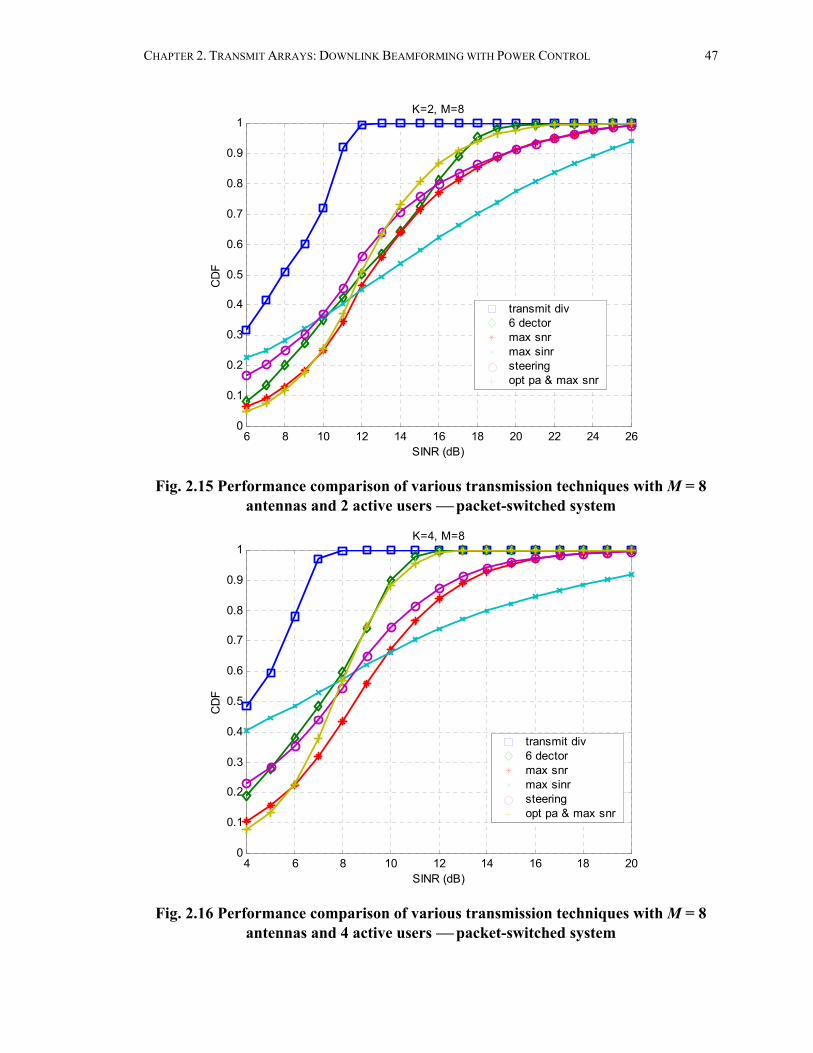
CHAPTER 2. TRANSMIT ARRAYS: DOWNLINK BEAMFORMING WITH POWER CONTROL 47
6 8 10 12 14 16 18 20 22 24 260
0.1
0.2
0.3
0.4
0.5
0.6
0.7
0.8
0.9
1K=2, M=8
SINR (dB)
CD
F
transmit div 6 dector max snr max sinr steering opt pa & max snr
Fig. 2.15 Performance comparison of various transmission techniques with M = 8
antennas and 2 active users packet-switched system
4 6 8 10 12 14 16 18 200
0.1
0.2
0.3
0.4
0.5
0.6
0.7
0.8
0.9
1K=4, M=8
SINR (dB)
CD
F
transmit div 6 dector max snr max sinr steering opt pa & max snr
Fig. 2.16 Performance comparison of various transmission techniques with M = 8
antennas and 4 active users packet-switched system

CHAPTER 2. TRANSMIT ARRAYS: DOWNLINK BEAMFORMING WITH POWER CONTROL 48
Table 2.2 Mean SINR (50% CDF) of a typical mobile user (dB)
Table 2.3 Peak SINR (90% CDF) of a typical mobile user (dB)
From the above data, several conclusions can be drawn for CDMA downlink packet-
switched systems.
• Optimal power allocation scheme has no benefit in packet-switched systems. We see
from Figs 2.14 to 2.16 that, the Max SNR with optimal power allocation, compared
with Max SNR with equal power allocation, favors low-rate (low SINR) users but
M=4 & K=2
M=8 & K=2
M=8 & K=4
TransmitDiversity
SixSector
BeamSteering
MaxSNR
MaxSNR(f)
MaxSINR
MaxSINR(f)
Opt PA& MaxSNR
Opt PA& MaxSNR(f)
8 11.8 10.8 11 11.1 10.6 10.8 10.6 10.7
8 12 11.4 12.4 12.7 13.2 13.7 11.9 12.3
4.2 7.2 7.6 8.5 8.8 6.4 7.2 7.7 8.2
TransmitDiversity
SixSector
BeamSteering
MaxSNR
MaxSNR(f)
MaxSINR
MaxSINR(f)
Opt PA& MaxSNR
Opt PA& MaxSNR(f)
11 17.5 15.5 15.7 15.7 21.6 21.6 13.8 13.8
10.8 17.2 19.3 19.5 19.5 24.3 24.6 16.8 17.1
6.8 10 12.7 13.3 13.4 18.8 19.3 10.3 10.6
M=4 & K=2
M=8 & K=2
M=8 & K=4

CHAPTER 2. TRANSMIT ARRAYS: DOWNLINK BEAMFORMING WITH POWER CONTROL 49
harms high-rate (high SINR) users. As we discussed in Section 2.3, optimal power
allocation is like a socialist scheme that seeks absolute fairness. It cannot achieve the
highest throughput and, without being jointly considered with the link and network
schedules, cannot guarantee fairness either. A similar phenomenon can be observed
for the Max SINR scheme and is omitted here.
• Contrary to the circuit case, Max SINR beamforming has the best performance in
terms of peak rate; it is also good at mean rate with small numbers of users, while
comparable with others when there are more users.
• Max SNR beamforming is almost the best in terms of mean rate; it is also good in
terms of peak rate performance.
• Beam steering is almost as good as max SNR in terms of peak rate performance,
while a little worse (1 dB) in terms of mean rate performance.
• For transmit diversity, sectorization significantly improves the performance (4-7 dB).
• The Max SNR beamforming technique outperforms the six-sector transmit diversity
scheme for M = 8 (1dB in mean and 2-3 dB in peak); for M = 4, six-sector transmit
diversity is better.
Figures 2.17 to 2.19 compare Max SNR beamforming with and without feedback,
while Figs. 2.20 to 2.22 show the Max SINR case. We find that feedback does not help
much for beamforming in packet-switched systems.

CHAPTER 2. TRANSMIT ARRAYS: DOWNLINK BEAMFORMING WITH POWER CONTROL 50
0 5 10 15 200
0.1
0.2
0.3
0.4
0.5
0.6
0.7
0.8
0.9
1K=2, M=4
SINR (dB)
CD
F
max snr w/o feedback max snr with feedback
Fig. 2.17 Performance of max SNR beamforming with 4 antennas and 2 active
users: with and without feedback channel information
0 5 10 15 200
0.1
0.2
0.3
0.4
0.5
0.6
0.7
0.8
0.9
1K=2, M=8
SINR (dB)
CD
F
max snr w/o feedback max snr with feedback
Fig. 2.18 Performance of max SNR beamforming with 8 antennas and 2 active
users: with and without feedback channel information

CHAPTER 2. TRANSMIT ARRAYS: DOWNLINK BEAMFORMING WITH POWER CONTROL 51
0 5 10 15 200
0.1
0.2
0.3
0.4
0.5
0.6
0.7
0.8
0.9
1K=4, M=8
SINR (dB)
CD
F
max snr w/o feedback max snr with feedback
Fig. 2.19 Performance of max SNR beamforming with 8 antennas and 4 active users: with and without feedback channel information
0 5 10 15 20
0.1
0.2
0.3
0.4
0.5
0.6
0.7
0.8
0.9
1K=2, M=4
SINR (dB)
CD
F
max sinr w/o feedback max sinr with feedback
Fig. 2.20 Performance of max SINR beamforming with 4 antennas and 2 active
users: with and without feedback channel information

CHAPTER 2. TRANSMIT ARRAYS: DOWNLINK BEAMFORMING WITH POWER CONTROL 52
0 5 10 15 200
0.1
0.2
0.3
0.4
0.5
0.6
0.7
0.8K=2, M=8
SINR (dB)
CD
F
max sinr w/o feedback max sinr with feedback
Fig. 2.21 Performance of max SINR beamforming with 8 antennas and 2 active
users: with and without feedback channel information
0 5 10 15 200.2
0.3
0.4
0.5
0.6
0.7
0.8
0.9
1K=4, M=8
SINR (dB)
CD
F
max sinr w/o feedback max sinr with feedback
Fig. 2.22 Performance of max SINR beamforming with 8 antennas and 4 active
users: with and without feedback channel information

CHAPTER 2. TRANSMIT ARRAYS: DOWNLINK BEAMFORMING WITH POWER CONTROL 53
2.6 Summary In this chapter, we have seen that traffic type impacts the algorithm choice in downlink
beamforming. For circuit-switched downlink CDMA systems, the Max SNR
beamforming scheme is the best choice (accommodating 12 to 42 more users than
transmit diversity). For packet-switched systems, Max SINR Beamforming has the best
performance in terms of peak rate (10-14 dB more than transmit diversity); Max SNR
beamforming is almost the best in terms of mean rate (3-4 dB more than transmit
diversity), but beam steering and transmit diversity with sectorization are also good
choices. We also see that sectorization greatly improves the system performance, both for
the circuit and for the packet case. For transmit diversity, the gain from exploiting more
antennas diminishes, while this is not the case for beamforming, especially with feedback
channel information. The following issues deserve further study in this context.
• In this chapter, we have assumed the perfect knowledge of DOA when calculating the
downlink spatial covariance matrix. The issue of parameter estimation errors in
covariance matrix calculation deserves further study.
• As we have noted, the optimal power allocation has no benefit on the packet-switched
systems. Combining link and network schedules with transmission techniques in
packet-switched systems is of interest.
• In this chapter, we have mainly studied array-processing techniques to combat the
small-scale fading. Their counterparts for widely separated antennas (macrodiversity)
are also of interest.

54
Chapter 3
Receive Arrays:
Iterative Space-Time Multiuser Detection
3.1 Introduction In this chapter, space-time multiuser detection for wireless communications with receive
arrays is studied. To overcome the computational burden that rises very quickly with
increasing numbers of users and receive antennas in asynchronous multipath CDMA
channels, efficient implementations of space-time multiuser detection algorithms,
including batch iterative methods and sample-by-sample adaptive methods, are
considered here.
The presence of both multiple-access interference (MAI) and intersymbol
interference (ISI) constitutes a major impediment to reliable high-data-rate CDMA
communications in multipath channels. These phenomena present challenges as well as
opportunities for receiver designers: through multiuser detection (MUD) [119] and space-
time (ST) processing [78], the inherent code, spatial, temporal and spectral diversities of
multipath multi-antenna CDMA channels can be exploited to achieve substantial gain.

CHAPTER 3. RECEIVE ARRAYS: ITERATIVE SPACE-TIME MULTIUSER DETECTION 55
Advanced signal processing typically improves system performance at the cost of
computational complexity. It is well known that the optimal maximum likelihood (ML)
multiuser detector has prohibitive computational requirements for most current
applications. A variety of linear and nonlinear multiuser detectors have been proposed to
ease this computational burden while maintaining satisfactory performance. However, in
asynchronous multipath CDMA channels with receive antenna arrays and large data
frame lengths, direct implementation of these suboptimal techniques still proves to be
very complex. Techniques for efficient space-time multiuser detection fall largely into
two categories. One includes batch iterative methods, which assume knowledge of all
signals and channels and is suitable, for example, for base station processing in cellular
systems. The other includes sample-by-sample adaptive methods, which require
knowledge only of the signal and (possibly) channel of a desired user. Sample-by-sample
adaptive methods are suitable both for mobile end processing, which entails decentralized
data detection, and for base station processing due to the time varying nature of wireless
communications. We may think of the sample-by-sample adaptive methods discussed
here as being most suitable for application at the base station, where it is more practical
to install an antenna array. However, most of the described decentralized or blind
techniques are readily applied to the mobile user end when multiple antennas can be
applied at mobile terminals.
This chapter is organized as follows. In Section 3.2 a space-time multiuser signal
model is presented. Batch iterative methods are discussed in Section 3.3 while sample-
by-sample adaptive methods are dealt with in Section 3.4. Numerical examples are given

CHAPTER 3. RECEIVE ARRAYS: ITERATIVE SPACE-TIME MULTIUSER DETECTION 56
in Section 3.3 and 3.4 to show the performance of the various iterative ST MUD
techniques developed in this chapter. Section 3.5 summarizes this chapter.
3.2 Space-Time Signal Model Consider a direct-sequence CDMA communication system with K users employing
normalized spreading waveforms 1, , Ks s… given by
1
0
1( ) ( ) ( ), 0 , 1 ,N
k k cj
s t c j t jT t T k KN
ψ−
=
= − ≤ ≤ ≤ ≤∑ (3.1)
where N is the processing gain, ( ); 0 1kc j j N≤ ≤ − is a signature sequence of 1± ’s
assigned to the kth user, and ( )ψ ⋅ is a normalized chip waveform of duration cT T N=
with T the symbol interval. User k (for 1 k K≤ ≤ ) transmits a frame of M independent
equiprobable BPSK symbols ( ) 1, 1kb i ∈ + − , 0 1i M≤ ≤ − ; and the symbol sequences
from different users are assumed to be mutually independent. The transmitted baseband
signal due to the kth user is thus given by
1
0
( ) ( ) ( ), 1 ,M
k k k ki
x t A b i s t iT k K−
=
= − ≤ ≤∑ (3.2)
where kA is the amplitude associated with user k’s transmission. The transmitted signal
of each user passes through a multipath channel before it is received by a uniform linear
antenna array (ULA) of P elements with inter-element spacing d. Then the single-input
multiple-output (SIMO) vector impulse response between the kth user and the receive
array can be modeled as

CHAPTER 3. RECEIVE ARRAYS: ITERATIVE SPACE-TIME MULTIUSER DETECTION 57
1
( ) ( ),L
k kl kl kll
t g tδ τ=
= −∑h a (3.3)
where L is the maximum number of resolvable paths between each user and the receive
array (for simplicity we assume L is the same for each user), klg and klτ are respectively
the complex gain and delay of the lth path of the kth user, and
,12 sin( ) /
,2
2 ( 1)sin( ) /,
1kl
kl
klj d
klkl
j d Pkl P
aa e
a e
π θ λ
π θ λ−
= =
a (3.4)
is the ULA response corresponding to the signal of the lth path of the kth user with
direction of arrival (DOA) klθ and carrier wavelength λ . ( )tδ denotes the Dirac delta
function. The received signal at the antenna array is the superposition of the channel-
distorted signals from the K users together with additive Gaussian noise, which is
assumed to be spatially and temporally white. This leads to the vector received signal
model
1
( ) ( ) ( ) ( ),K
k kk
t x t t tσ=
= ⊗ +∑r h n (3.5)
where ⊗ denotes convolution, and 2σ is the spectral height of the ambient Gaussian
noise at each antenna element.
A sufficient statistic for demodulating the multiuser symbols from the space-time
signal (3.5) is given by [127]
1 1 1[ (0), , (0), (1), , ( 1), , ( 1)] ,TK Ky y y y M y M= − −y … … … (3.6)

CHAPTER 3. RECEIVE ARRAYS: ITERATIVE SPACE-TIME MULTIUSER DETECTION 58
where the elements ( )ky i are defined as follows:
*
1( )
( ) ( ) ( ) , 1 , 0 1
kl
LH
k kl kl k kll
i
y i g t s t iT dt k K i Mτ∞
−∞=
= − − ≤ ≤ ≤ ≤ −∑ ∫z
a r . (3.7)
To produce this sufficient statistic, the received signal vector ( )tr is first match-filtered
for each path of each user to form the vector observables ( )klz i , after which beams are
formed on each path of each user via the dot products with the array responses kla , and
then all the paths of each user are combined with a RAKE receiver. This process
produces one observable for each symbol of each user. Since the system is in general
asynchronous and the users are not orthogonal, we need to collect the statistic for all
users over the entire data frame. The observable ( )ky i corresponds to the output of a
conventional space-time matched filter, matched to the ith symbol of user k. Therefore, a
general space-time multiuser receiver is (as shown in Fig. 3.1) a space-time matched
filter bank, followed by a decision algorithm. In the following, we will present various
ST MUD receivers based on this space-time matched filter output. However, a new ST
MUD receiver structure will also be introduced, in which chip-level observables are
exploited.
The sufficient statistic (3.6) can be written as (see [119])
,σ= +y HAb v (3.8)
where H is a KM KM× matrix capturing the cross-correlations between different
symbols and different users, A is the KM KM× diagonal matrix whose k iK+ diagonal
elements are equal to kA , 1 1 1[ (0), , (0), (1), , ( 1), , ( 1)]TK Kb b b b M b M= − −b … … … , and

CHAPTER 3. RECEIVE ARRAYS: ITERATIVE SPACE-TIME MULTIUSER DETECTION 59
~ (0, )v HN (i.e., v is Gaussian with zero mean and covariance matrix H). An optimal
ML space-time multiuser detector will maximize the following log-likelihood function
( ) 2Re T TΩ = −b b Ay b AHAb . (3.9)
Decision Algorithm
Fig. 3.1 A conventional space-time multiuser receiver structure The multiuser signal and channel parameters (signature waveforms, multipath delay and
amplitude, array response) come into play through the KM KM× block Toeplitz system
matrix H, which can be written as
[0] [1] [ ]
[ 1] [0] [1] [ ]
[ ] [0] [ ]
[ ] [ 1] [0] [1]
[ ] [ 1] [0]
,
H H H
H H H H
H H H
H H H H
H H H
∆
− ∆
−∆ ∆
−∆ −
−∆ −
H (3.10)
CHAPTER 3. RECEIVE ARRAYS: ITERATIVE SPACE-TIME MULTIUSER DETECTION 60
where ∆ denotes the multipath delay spread, and [ ] [ ]( )i i HH H− = . The n, mth element of
H is the cross-correlation between the composite received signatures (after beamforming
and RAKE combining) of the nth and mth elements of b. The reader is referred to [127]
for further details of H. Dynamic programming can be applied to compute the ML
estimates of b. Due to the binary nature of b, the complexity of this computation is on the
order of ( 1)(2 / )KO K∆+ per user per symbol.
3.3 Batch Iterative Methods There has been considerable research in space-time processing (e.g., [67], [78]), most of
which considers single-user-based methods. Combined multiuser detection and array
processing has been addressed recently (e.g. [72], [127]). In this section, we consider
iterative implementation of linear and nonlinear space-time multiuser detectors (ST
MUD) in multipath CDMA channels with receive antenna arrays. In particular, we
develop several such algorithms, and compare them on the basis of performance and
complexity. Ultimately, we conclude that an algorithm based on the expectation-
maximization (EM) algorithm offers an attractive tradeoff in this context.
3.3.1 Iterative Linear ST MUD In this part, we consider the application of iterative processing to the implementation of
various linear space-time multiuser detectors in algebraic form. After the introduction to
the general form of linear ST MUD, we go on to discuss two general approaches to

CHAPTER 3. RECEIVE ARRAYS: ITERATIVE SPACE-TIME MULTIUSER DETECTION 61
iteratively solving large systems of linear equations. Subsequent subsections will treat
nonlinear iterative methods.
Linear multiuser detectors in the framework of (3.8) are of the form
ˆ sgn(Re )=b Wy , (3.11)
where W is a KM KM× matrix. For the linear decorrelating (zero-forcing) detector, this
matrix is given by
1d
−=W H , (3.12)
while for the linear MMSE detector, we have
2 2 1( ) .m σ − −= +W H A (3.13)
Direct inversion of the matrices in (3.12) and (3.13) (after exploiting the block Toeplitz
structure) is of complexity 2( )O K M∆ per user per symbol [48].
The linear multiuser detection estimates of (3.11) can be seen as the solution of a
linear equation
=Cx y , (3.14)
with =C H for the decorrelating detector and 2 2σ −= +C H A for the MMSE detector.
Jacobi and Gauss-Seidel iteration are two common low-complexity iterative schemes for
solving linear equations such as (3.14) [48]. If we decompose the matrix C as
L U= + +C C D C where LC denotes the lower triangular part, D denotes the diagonal
part, and UC denotes the upper triangular part, then Jacobi iteration can be written as
1 11( )m L U m
− −−= − + +x D C C x D y , (3.15)

CHAPTER 3. RECEIVE ARRAYS: ITERATIVE SPACE-TIME MULTIUSER DETECTION 62
and Gauss-Seidel iteration is represented as
1 11( ) ( ) .m L U m L
− −−= − + + +x D C C x D C y (3.16)
From (3.15), Jacobi iteration can be seen to be a form of linear parallel interference
cancellation [89], the convergence of which is not guaranteed in general. One of the
sufficient conditions for the convergence of Jacobi iteration is that ( )L U− +D C C be
positive definite [48]. In contrast, Gauss-Seidel iteration, which (3.16) reveals to be a
form of linear serial interference cancellation, converges to the solution of the linear
equation from any initial value, under the mild conditions that C is symmetric and
positive definite [48], which is always true for the MMSE detector.
Another approach to solving the linear equation (3.14) involves gradient methods,
among which are steepest descent and conjugate gradient iteration [48]. The reader is
referred to Section 3.4 for sample-by-sample adaptive space-time processing methods,
which apply gradient methods in a different setting. Note that solving (3.14) is equivalent
to minimizing the cost function
1( ) .2
H HΦ = −x x Cx x y (3.17)
The idea of gradient methods is the successive minimization of this cost function along a
set of directions mp via
1 ,m m m mα−= +x x p (3.18)
with
1 ,H Hm m m m mα −= p q p Cp (3.19)

CHAPTER 3. RECEIVE ARRAYS: ITERATIVE SPACE-TIME MULTIUSER DETECTION 63
and
( ) .mm m== −∇Φ = −x xq x y Cx (3.20)
Different choices of the set mp in (3.18) - (3.20) give different algorithms. If we choose
the search directions mp to be the negative gradient of the cost function 1m−q directly,
this algorithm is the steepest descent method, global convergence of which is guaranteed
[48]. The convergence rate may be prohibitively slow, however, due to the linear
dependence of the search directions, resulting in redundant minimization. If we choose
the search direction to be C-conjugate as follows
1
1 ,argminm
m m⊥−
−∈Λ
= −p
p p q (3.21)
where 1span ,...,m mΛ = Cp Cp , then we have the conjugate gradient method, whose
convergence is guaranteed and performs well when C is near the identity either in the
sense of a low rank perturbation or in the sense of norm [48]. The computational
complexity of Gauss-Seidel and conjugate gradient iteration are similar, which is on the
order of ( )O K m∆ per user per symbol, where m is the number of iterations.
3.3.2 Iterative Nonlinear ST MUD Nonlinear multiuser detectors are often based on bootstrapping techniques, which are
iterative in nature. In this part, we will consider the iterative implementation of decision-
feedback multiuser detection in the space-time domain. We also discuss briefly the
implementation of multistage interference cancelling ST MUD, which serves as a

CHAPTER 3. RECEIVE ARRAYS: ITERATIVE SPACE-TIME MULTIUSER DETECTION 64
reference point for introducing a new EM-based iterative ST MUD, to be discussed in the
next subsection.
3.3.2.1 Cholesky Iterative Decorrelating Decision-Feedback ST MUD Decorrelating decision feedback multiuser detection (DDF MUD) [34], [117] exploits the
Cholesky decomposition H=H F F , where F is a lower triangular matrix, to determine
feedforward and feedback matrices for detection via the algorithm
ˆ ˆsgn( ( diag( )) )),H−= − −b F y F F Ab (3.22)
which should be understood to detect the bits sequentially from that of the first user to the
last user, with b a vector containing the detected bits for all users over the whole data
frame.
Suppose the user of interest is user k (each bit of each user can be treated as a “new”
user for asynchronous systems), the purpose of the feedforward matrix H−F is to whiten
the noise and decorrelate against the “future users” 1 , , k KMs s+ … ; while the purpose of
the feedback matrix ( diag( ))−F F is to cancel out the interference from “previous users”
1 1 , , ks s −… . Note that the performance of DDF MUD is not uniform. While the first user
is demodulated by its decorrelating detector, the last detected user will essentially achieve
its single-user lower bound providing the previous decisions are correct. There is another
form of Cholesky decomposition, in which the feedforward matrix F is upper triangular.
If we were to use this form instead in (3.22), then the multiuser detection would be in the
reverse order, as would be the performances. The idea of Cholesky iterative DDF ST

CHAPTER 3. RECEIVE ARRAYS: ITERATIVE SPACE-TIME MULTIUSER DETECTION 65
MUD is to employ these two forms of Cholesky decomposition alternatively as follows.
For lower triangular Cholesky decomposition 1F , first feedforward filtering is applied as
1 1 ,H−=y F y (3.23)
where it is readily shown that 1
1, 1, 1, 1,1
i
i ii i i ij j j ij
y Ab A b n−
=
= + +∑F F , 1, ,i KM= … , with 1,in ,
1, ,i KM= … , the independent and identically distributed (i.i.d.) Gaussian noise
components with zero mean and variance 2σ . We can see that the influence of the
“future users” is eliminated and the noise component is whitened. Then we employ the
feedback filtering to take out the interference from “previous users” as
1 1 1 1ˆ ,= − −u y (F diag(F ))Ab (3.24)
where it is easily seen that 1
1, 1, 1, 1, 1,1
ˆi
i i ij j j ii i i ij
u y A b Ab n−
=
= − ≈ +∑F F , 1, ,i KM= … . Similarly,
for upper triangular Cholesky decomposition 2F , we have
2 2 ,H−=y F y (3.25)
where 2, 2, 2, 2,1
KM
i ii i i ij j j ij i
y Ab A b n= +
= + +∑F F , , ,1i KM= … , and
2 2 2 2ˆ ,= − −u y (F diag(F ))Ab (3.26)
where 2, 2, 2, 2, 2,1
ˆKM
i i ij j j ii i i ij i
u y A b Ab n= +
= − ≈ +∑ F F , , ,1i KM= … .
After the above operations are (alternately) executed, the following log-likelihood
ratio is calculated,

CHAPTER 3. RECEIVE ARRAYS: ITERATIVE SPACE-TIME MULTIUSER DETECTION 66
* 21/ 2, 1/ 2,2 Re( ) / ,i ii i iL Au σ= F (3.27)
where 1/ 2F and 1/ 2u are used to give a shorthand representation for both alternatives.
Then the log-likelihood ratio is compared with the last stored value, which is replaced by
the new value if the new one is more reliable, i.e.,
.stored stored newi i istored
i newi
L if L LL
L otherwise
>=
(3.28)
Finally, we make soft decisions ˆ tanh( / 2)i ib L= at an intermediate iteration, which has
been shown to offer better performance than making hard intermediate decisions, and
make hard decisions ˆ sgn( )i ib L= at the last iteration. Three or four iterations are usually
enough for the system to achieve an improved steady state without significant oscillation.
The structure of Cholesky iterative decorrelating decision-feedback ST MUD is
illustrated in Fig. 3.2.
F1
F2
1y
2y
12
i
KM
12
i
KM
Log-likelihood ratio: Li Estimates: ib
)2/tanh(ˆii Lb =
)sgn(ˆii Lb =
Fig. 3.2 Cholesky iterative decorrelating decision-feedback ST MUD

CHAPTER 3. RECEIVE ARRAYS: ITERATIVE SPACE-TIME MULTIUSER DETECTION 67
The Cholesky factorization of the block Toeplitz matrix H (see (3.10)) can be done
recursively. For 1∆ =
1
2 2
0 0 0 01 0 0 0
0
0 0 1 0M M
F ( )F ( ) F ( )
F ( ) F ( )
=
F , (3.29)
where the element matrices are obtained recursively as follows:
[0] ,MV H= (3.30)
and, for , 1, ,1i M M= − … , we do the Cholesky decomposition for the reduced-rank
matrix iV to get (0)iF
(0) (0),Hi iiV F F= (3.31)
while (1)iF is obtained as
[ 1]1(1) ( (0))Hi iF F H −−= . (3.32)
Finally we have
[0] [1] 1 [ 1]1i iV H H V H− −− = − (3.33)
for use in the next iteration. The extension of this algorithm to 1∆ > is straightforward
and is omitted here.

CHAPTER 3. RECEIVE ARRAYS: ITERATIVE SPACE-TIME MULTIUSER DETECTION 68
3.3.2.2 Multistage Interference Cancelling ST MUD Multistage interference cancellation (IC) [115] is similar to Jacobi iteration except that
hard decisions are made at the end of each stage in place of the linear terms that are fed
back in (3.15). Thus we have
( ) ( )1 1ˆ ˆ ˆsgn ( ) sgn ( )m L U m m− −= − + = − −b y C C b y H D b . (3.34)
The underlying rationale of this method is that the estimator-subtracter structure exploits
the discrete-alphabet property of the transmitted data streams. This nonlinear hard-
decision operation typically results in more accurate estimates, especially in high SNR
situations. Although the optimal decisions are a fixed point of the nonlinear
transformation (3.34), there are problems with the multistage IC such as a possible lack
of convergence and oscillatory behavior. In the following section we consider some
improvement over space-time multistage IC MUD.
Except for the Cholesky factorization, the computational complexity for Cholesky
iterative DDF ST MUD is the same as multistage IC ST MUD, which is essentially the
same as that of linear interference cancellation, i.e., ( )O K m∆ per user per symbol.
3.3.3 EM-based Iterative ST MUD with a New Structure In this part, EM and space-alternating generalized EM (SAGE) algorithms are applied to
the space-time multipath asynchronous CDMA systems to avoid the convergence and
stability problem of the multistage IC MUD. To address the problems caused by long
spreading codes, namely, the large computational burden to obtain the cross-correlation
matrix H, a new space-time multiuser receiver structure is also introduced. The SAGE
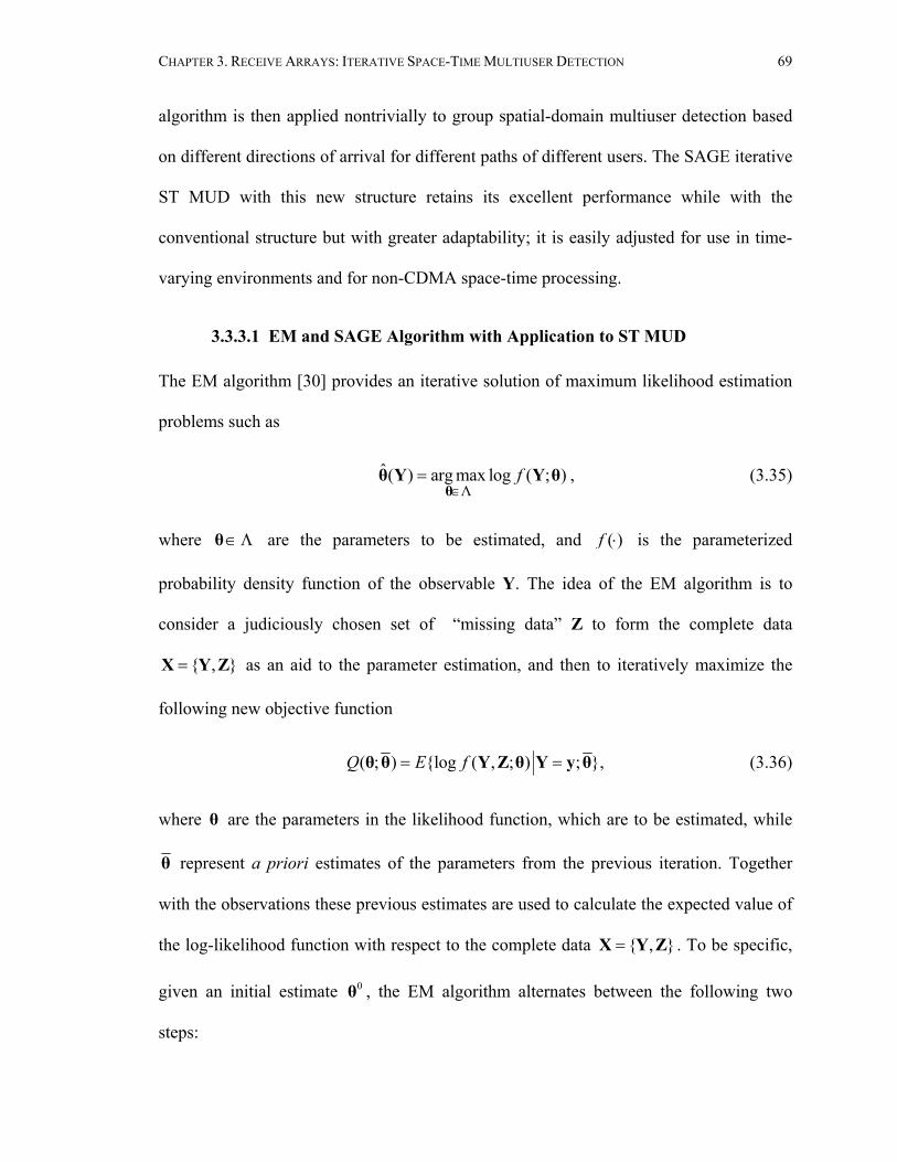
CHAPTER 3. RECEIVE ARRAYS: ITERATIVE SPACE-TIME MULTIUSER DETECTION 69
algorithm is then applied nontrivially to group spatial-domain multiuser detection based
on different directions of arrival for different paths of different users. The SAGE iterative
ST MUD with this new structure retains its excellent performance while with the
conventional structure but with greater adaptability; it is easily adjusted for use in time-
varying environments and for non-CDMA space-time processing.
3.3.3.1 EM and SAGE Algorithm with Application to ST MUD The EM algorithm [30] provides an iterative solution of maximum likelihood estimation
problems such as
Λ
ˆ( ) arg max log ( ; )f∈
=θ
θ Y Y θ , (3.35)
where ∈Λθ are the parameters to be estimated, and ( )f ⋅ is the parameterized
probability density function of the observable Y. The idea of the EM algorithm is to
consider a judiciously chosen set of “missing data” Z to form the complete data
, =X Y Z as an aid to the parameter estimation, and then to iteratively maximize the
following new objective function
( ; ) log ( , ; ) ; ,Q E f= =θ θ Y Z θ Y y θ (3.36)
where θ are the parameters in the likelihood function, which are to be estimated, while
θ represent a priori estimates of the parameters from the previous iteration. Together
with the observations these previous estimates are used to calculate the expected value of
the log-likelihood function with respect to the complete data , =X Y Z . To be specific,
given an initial estimate 0θ , the EM algorithm alternates between the following two
steps:

CHAPTER 3. RECEIVE ARRAYS: ITERATIVE SPACE-TIME MULTIUSER DETECTION 70
(a). E-step, where the complete-data sufficient statistic ( ; )iQ θ θ is computed;
(b). M-step, where the estimates are refined by 1 arg max ( ; )i iQ+
∈Λ=
θθ θ θ .
It is well known that EM estimates monotonically increase the likelihood, and converge
stably to an ML solution under certain conditions [30].
An issue in using the EM algorithm is the tradeoff between ease of implementation
and convergence rate. One would like to add more “missing data” to make the complete
data space more informative so that the implementation of the EM algorithm is simpler
than the original setting (3.35). However, the convergence rate of the algorithm is
inversely proportional to the Fisher information contained in the complete data space
[38]. Thus, the convergence rate of the EM algorithm is notoriously slow, especially for
multidimensional parameter estimation, due to the simultaneous updating nature of the
M-step of the EM algorithm. The SAGE algorithm has been proposed in [38] to improve
the convergence rate for multidimensional parameter estimation. The idea is to divide the
parameters into several groups (subspaces), with only one group being updated at each
iteration. Thus, we can associate multiple less-informative “missing data” sets to improve
the convergence rate while maintaining overall tractability of optimization problems. For
each iteration, a subset of parameters iSθ and the corresponding missing data iSZ are
chosen, which is called the definition step. Then similar to the EM algorithm, in the E-
step we calculate
,( ; ) log ( , ; ; ),i i
i i i
S Si i iS S SQ E f= =θ θ Y Z θ θ Y y θ (3.37)
where iSθ denotes the complement of
iSθ in the whole parameter set; in the M-step, the
chosen parameters are updated while the others remain unchanged as

CHAPTER 3. RECEIVE ARRAYS: ITERATIVE SPACE-TIME MULTIUSER DETECTION 71
1
θ Λ
1
arg max ( ; ),
i
i iS Si i
i i
Si iS S
i iS S
Q+
∈
+
=
=
θ θ θ
θ θ (3.38)
where iSΛ denotes the restriction of the entire parameter space to those dimensions
indexed by iS . Like the traditional EM estimates, the SAGE estimates also monotonically
increase the likelihood and converge stably to an ML solution [38].
The EM algorithm can be applied to space-time multipath asynchronous CDMA
multiuser detection as follows. For ease of illustration, we reindex the vectors and
matrices in the system model (3.8) as
1 1 ( 1) 1[ , , , , , , , ] ,TK K K M KMy y y y y+ − +=y … … …
1 1 ( 1) 1[ , , , , , , , ] ,TK K K M KMb b b b b+ − +=b … … …
and 1 1 ( 1) 1diag[ , , , , , , , ] .T
K K K M KMa a a a a+ − +=A … … …
Suppose we would like to detect a bit kb , 1,2, , k KM∈ , while the interfering users’
bits j j kk b ≠=b are treated as the missing data. The complete-data sufficient statistic is
given by ( kmH is the element of matrix H at the kth row and mth column)
2
22( ; ) 2 ( ) ,
2i k k
k k k k km m mm kk
a bQ b b b y a baσ ≠
= − + − ∑
H (3.39)
with
2 | ; tanh( ( )),i imm m k k m mk k k
ab E b b b y a bσ
= = = = −Y y H (3.40)

CHAPTER 3. RECEIVE ARRAYS: ITERATIVE SPACE-TIME MULTIUSER DETECTION 72
which forms the E-step of the EM algorithm. The M-step is given by
1
sgn( ) 1arg max ( ; ) ,1 ( )k
k km m mm k
i ik k kb
k km m mm kk
y a bb Q b b
y a ba
≠+
∈Λ
≠
− Λ = ±∑
= = − Λ =ℜ∑
H
H (3.41)
where Λ =ℜ (the set of real numbers) means a soft decision is needed, e.g., in an
intermediate stage. Note that in the E-step (40), interference from users j k≠ is not taken
into account, since these are treated as “missing data”. This shortcoming is overcome by
the application of the SAGE algorithm, where the bit vector of all users 1 KMj jb ==b is
treated as the parameter to be estimated and no missing data is needed. The algorithm is
described as follows: for 0,1, ,i =
Definition step: 1 ( mod )iS i KM= +
M-step:1
1
sgn( )i ik k km m m i
m ki im m i
b y a b k S
b b m S
+
≠+
= − ∈∑
= ∉
H. (3.42)
Note that there is no E-step since there is no missing data, and interference from all other
users is recreated from previous estimates and subtracted. The resulting receiver is
similar to the multistage interference cancelling multiuser receiver (see (3.34)), except
that the bit estimates are made sequentially rather than in parallel. However, with this
simple concept of sequential interference cancellation, the resulting multiuser receiver is
convergent, guaranteed by the SAGE algorithm. The multistage interference cancelling
multiuser receiver discussed in 3.3.2.2, on the other hand, does not always converge. The
computational complexity of this SAGE iterative ST MUD is also ( )O K m∆ per user per
symbol.

CHAPTER 3. RECEIVE ARRAYS: ITERATIVE SPACE-TIME MULTIUSER DETECTION 73
3.3.3.2 SAGE Iterative ST MUD with a New Structure So far when we discuss computational complexity, we have ignored the computational
burden for calculating the matrix H. In a CDMA system exploiting short spreading codes
as we have assumed, the system matrix will exhibit the block-Toeplitz structure as shown
in (10). The computation of [ ]jH , 1 j≤ ≤ ∆ , though involved (please see [127] for
details), would become insignificant when M is large. This is not the case, however, when
a long spreading code is employed so that spreading sequences vary from symbol to
symbol (e.g. in IS-95). In this situation, the sub-matrices [ ]jH , 1 j≤ ≤ ∆ , have to be
calculated for each symbol, which results in an additional complexity of 3 3( )O K L ∆ per
user per symbol.
CMF11
1L
K1
KL
11
1L
K1
KL
RAKE
User 1
User 2
User K
BeamformingSuccessive Cancellation
RAKE
Despreading
User 1
User 2
User K
Remodulation
Received Signal
Estimated Interference
Spatial Signature Spreading waveform
Fig. 3.3 A new space-time multiuser receiver structure

CHAPTER 3. RECEIVE ARRAYS: ITERATIVE SPACE-TIME MULTIUSER DETECTION 74
To circumvent this problem, a new space-time processing structure is introduced,
where we separate the spatial and temporal processing, and apply the SAGE algorithm to
spatial-domain multiuser detection based on different directions of arrival for different
paths of different users, as shown in Fig. 3.3.
From (3.5), we can write
1
0 1 1( ) ( ) ( ) ( ).
M K L
k k kl kl k kli k l
t A b i g s t iT tτ σ−
= = =
= − − +∑∑ ∑r a n (3.43)
After chip-matched filtering and chip-rate sampling, the discrete time signal is given as
min
min
( 1) max minmin( ) ( ) ( ) , 0 1 ,c
c
n T
cnTc
n t t nT dt n MNT
τ
τ
τ τψ τ+ +
+
−= − − ≤ ≤ − +
∫z r (3.44)
where minτ and maxτ denote the minimum and maximum value, respectively, of the delay
profile for all users. For simplicity, we assume the delays are integer numbers of chip
intervals. (The results can straightforwardly be extended to the fractional delay case by
oversampling.) On denoting
min
min
1( 1)
min0
( ) ( ) ( ) ,c
c
Mn T
kl k kl cnTi
s n s t iT t nT dtτ
ττ ψ τ
−+ +
+=
= − − − −∑∫ (3.45)
we have
min
1 1( ) ( ) ( )
( ) ( ), 1 ,
K Lkl
k k kl kl klk l c
j j jj
n A b n N g s n nT
A d n n j K L
τ τ σ
σ
−
= =
= + + = + ≤ ≤ ×
∑∑
∑
z a e
a e (3.46)

CHAPTER 3. RECEIVE ARRAYS: ITERATIVE SPACE-TIME MULTIUSER DETECTION 75
where for the last equality we reformulate the system model so that chips received from
different paths of each user are treated as different users in a synchronous system,
according to the following translation
, , and ,j k kl j kl j k klA A g d b s↔ ↔ ↔a a (3.47)
with ( 1)* ,j k L l= − + 1 k K≤ ≤ , 1 l L≤ ≤ . Here ( )ne denotes i.i.d. white background
noise with zero mean and unit variance. The parameters to be estimated are
1[ ( ), , ( )] 1T KLK Ld n d n×= = ∈ ±θ d … which correspond to the chips from all paths of all
users. The index sets cycle through 1, , KL… , with L chips (of a user) being updated at a
time. The algorithm is implemented without any missing data so there is no need for the
E-step. Each iteration thus comprises the following steps:
Definition step: [1, , ] ( mod )iS L i K L= + × ;
M-step: 1
1
( )
,
i H ij j m m m i
m j
i im m i
d g A d j S
d d m S
+Λ
≠
+
= − ∈
= ∉
∑a z a. (3.48)
Since the spatial processing is one of the components of our proposed space-time
receiver, whose outputs are provided to the next stage for temporal processing, we choose
to use the linear function ( )g x xΛ = in the above M-step to produce soft outputs ( )jd n ,
ij S∈ , which is better for overall performance than the hard-decision function
( ) sgn( )g x xΛ = .

CHAPTER 3. RECEIVE ARRAYS: ITERATIVE SPACE-TIME MULTIUSER DETECTION 76
After the spatial processing described above, the chips from the different paths of one
user are combined through a RAKE combiner to get a chip estimate for that user
( ( mod )k i K= ),
* * max min
1
ˆ ( ) ( / ), 0 1 ,L
k k kl kl kl cl c
d n A g d n T n MNT
τ ττ=
−= + ≤ ≤ − +
∑ (3.49)
where the index conversion is made through the translation of (3.47). Finally, the
spreading code is employed to get the bit estimate
*
1
ˆ ˆ( ) sgn Re ( ) ( ) , 0 1N
k k kn
b i d iT n c n i M=
= + ≤ ≤ −
∑ . (3.50)
The obtained bit estimates are then respread and remodulated as (3.46) and (3.47) to get
1ijd + , ij S∈ for spatial domain interference cancellation (3.48) for the next iteration.
Our proposed space-time multiuser receiver structure in Fig. 3.3 has several
advantages. As we mentioned earlier, the multiuser signals and multipath channel
parameters come into play through the system matrix H. For a CDMA system employing
long spreading codes, H must be calculated for each symbol interval, which is quite
cumbersome. More generally, for any time-varying communication system, H has to be
updated on the order of the coherence time. Furthermore, any part of the algorithm that is
related to this system matrix, e.g., the Cholesky factorization for Cholesky iterative DDF
ST MUD, should also be calculated for each symbol. This problem is circumvented by
our structure, which effectively distributes the operations combined in the system matrix
H into the different stages of spatial IC, beamforming, temporal RAKE combining, and
despreading. Further, since the front end processing is at the chip level, these “users” are

CHAPTER 3. RECEIVE ARRAYS: ITERATIVE SPACE-TIME MULTIUSER DETECTION 77
synchronous. Therefore, the algorithm can be implemented chip-by-chip or symbol-by-
symbol in a pipelined version. This structure also has the benefit that it can be applied in
non-CDMA (e.g. space-division multiple-access (SDMA)) cellular networks to exploit
the spatial and temporal knowledge to suppress interference and improve system
capacity. All we need in such cases is to omit the despreading stage.
The computational complexity of this new-structure-based SAGE iterative ST MUD
is 2( )O KNL m per user per symbol, which can easily be implemented with ( )O KLm or
even less time complexity per user per symbol with modern VLSI techniques. The basic
idea would be to build multiple parallel hardware processing units, which can be done
due to the synchronous chip-level processing nature of the new structure. The multistage
IC ST MUD can also be implemented with this structure in a straightforward way. The
performance of these ST MUD receivers with this new structure is the same as that
implemented with the conventional structure of Fig. 3.1, which will be discussed further
in the next section.
3.3.4 Numerical Results In this section, the performance of the above described space-time multiuser detectors is
examined through computer simulations. We assume a K = 8-user CDMA system with
spreading gain N = 16. Each user travels through L = 3 paths before it reaches a ULA
with P = 3 elements and half-wavelength spacing. The maximum delay spread is set to be
1∆ = . The complex gains and delays of the multipath and the directions of arrival are
randomly generated and kept fixed for the whole data frame. This corresponds to a slow
fading situation. The spreading codes of all users are randomly generated and kept fixed

CHAPTER 3. RECEIVE ARRAYS: ITERATIVE SPACE-TIME MULTIUSER DETECTION 78
for all the simulations. We assume 1 KA A= =… for simplicity, but the received signal
powers of different users are unequal due to the effects of multipath.
First we compare the performance of various space-time multiuser receivers and
some single-user space-time receivers in Fig. 3.4. Five receivers are considered: the
single-user matched filter, the single-user MMSE receiver, the multiuser MMSE receiver
implemented in Gauss-Seidel or conjugate gradient iteration method (the performance is
the same for both), the Cholesky iterative decorrelating decision-feedback multiuser
receiver, and the multistage interference cancelling multiuser receiver. All these receivers
are implemented on the conventional space-time multiuser receiver structure shown in
Fig. 3.1. (The reader is referred to [127] for derivations of the single-user based
receivers.) The performance is evaluated after the iterative algorithms converge. Due to
the bad convergence behavior of the multistage IC MUD, we measure its performance
after three stages. The single-user lower bound is also depicted for reference. We can see
that the multiuser approach greatly outperforms the single-user based methods; nonlinear
MUD offers further gain over the linear MUD; and the multistage IC seems to approach
the optimal performance (not always, e.g., see Fig. 3.4(c)), when it has good convergence
behavior. Note that due to the introduction of spatial (receive antenna) and spectral
(RAKE combining) diversity, the SNR for the same BER is substantially lower than that
required by normal receivers without these signal processing methods.
Figure 3.5 shows the performance of Cholesky iterative decorrelating decision-
feedback ST MUD for two users, which is also typical for other users. Note that we use a
different parameter set for this simulation, so there is no correspondence between Fig. 3.4
and Fig. 3.5. We find that the Cholesky iterative method offers uniform gain over its non-

CHAPTER 3. RECEIVE ARRAYS: ITERATIVE SPACE-TIME MULTIUSER DETECTION 79
iterative counterpart. This gain may be substantial for some users and negligible for
others due to the individual characteristics of signals and channels.
In Section 3.3.3.2, a new space-time multiuser receiver structure was introduced to
reduce complexity and enhance adaptability of the algorithms while keeping the same
performance. In this new structure, different paths of each user are treated as separate
users in a synchronous system, while in the original structure, different paths are
combined prior to interference cancellation. One may be concerned that the new structure
is more susceptible to saturation (“dimensional crowding”) than the traditional structure
by a factor of L. We implemented the SAGE ST MUD with both structures for a fully
loaded 16K N= = system. The results shown in Fig. 3.6 are measured after three
iterations. It is seen that the performance is almost identical for these two structures. We
0 1 2 3 4 5 610
-4
10-3
10-2
10-1
SNR(dB)
Bit
erro
r rat
e
User #4
Matched-Filter SU MMSE MU MMSE Cholesky iterative MU DFMU Multistage Single User Bound MU Multistage IC
(a)

CHAPTER 3. RECEIVE ARRAYS: ITERATIVE SPACE-TIME MULTIUSER DETECTION 80
0 1 2 3 4 5 6 710
-5
10-4
10-3
10-2
10-1
SNR(dB)
Bit
erro
r rat
e
User #5
Matched-Filter SU MMSE MU MMSE Cholesky iterative MU DFMU Multistage Single User Bound MU Multistage IC
(b)
0 1 2 3 4 5 610
-5
10-4
10-3
10-2
10-1
SNR(dB)
Bit
erro
r rat
e
User #7
Matched-Filter SU MMSE MU MMSE Cholesky iterative MU DFMU Multistage IC Single User Bound
(c)
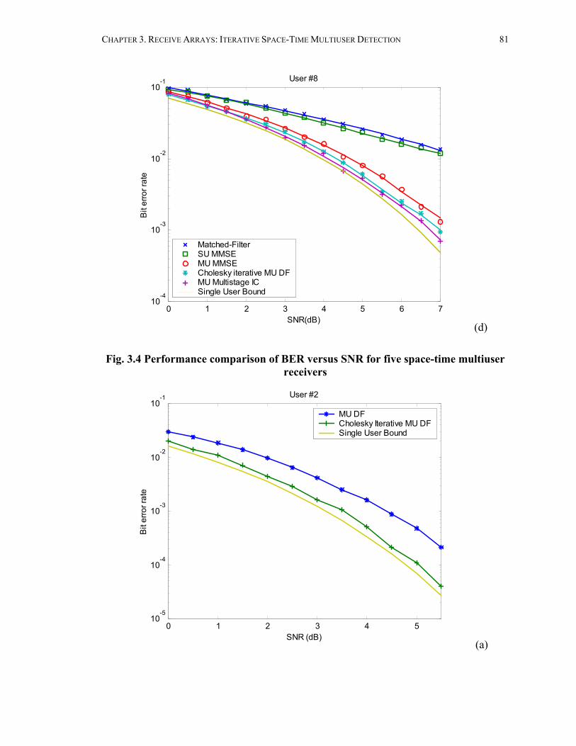
CHAPTER 3. RECEIVE ARRAYS: ITERATIVE SPACE-TIME MULTIUSER DETECTION 81
0 1 2 3 4 5 6 710
-4
10-3
10-2
10-1
SNR(dB)
Bit
erro
r rat
e
User #8
Matched-Filter SU MMSE MU MMSE Cholesky iterative MU DFMU Multistage IC Single User Bound
(d)
Fig. 3.4 Performance comparison of BER versus SNR for five space-time multiuser receivers
0 1 2 3 4 510
-5
10-4
10-3
10-2
10-1 User #2
SNR (dB)
Bit
erro
r rat
e
MU DF Cholesky Iterative MU DFSingle User Bound
(a)
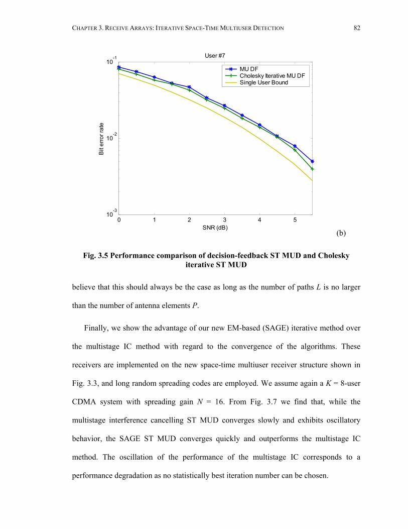
CHAPTER 3. RECEIVE ARRAYS: ITERATIVE SPACE-TIME MULTIUSER DETECTION 82
0 1 2 3 4 510
-3
10-2
10-1 User #7
SNR (dB)
Bit
erro
r rat
e
MU DF Cholesky Iterative MU DFSingle User Bound
(b)
Fig. 3.5 Performance comparison of decision-feedback ST MUD and Cholesky iterative ST MUD
believe that this should always be the case as long as the number of paths L is no larger
than the number of antenna elements P.
Finally, we show the advantage of our new EM-based (SAGE) iterative method over
the multistage IC method with regard to the convergence of the algorithms. These
receivers are implemented on the new space-time multiuser receiver structure shown in
Fig. 3.3, and long random spreading codes are employed. We assume again a K = 8-user
CDMA system with spreading gain N = 16. From Fig. 3.7 we find that, while the
multistage interference cancelling ST MUD converges slowly and exhibits oscillatory
behavior, the SAGE ST MUD converges quickly and outperforms the multistage IC
method. The oscillation of the performance of the multistage IC corresponds to a
performance degradation as no statistically best iteration number can be chosen.

CHAPTER 3. RECEIVE ARRAYS: ITERATIVE SPACE-TIME MULTIUSER DETECTION 83
0 1 2 3 4 510
-5
10-4
10-3
10-2
10-1 User #2
SNR (dB)
Bit
erro
r rat
e
SAGE traditionalSAGE new
(a)
0 1 2 3 4 5 6 710
-4
10-3
10-2
10-1 User #11
SNR (dB)
Bit
erro
r rat
e
SAGE traditionalSAGE new
(b)
Fig. 3.6 Performance comparison of SAGE ST MUD with traditional and new ST structure

CHAPTER 3. RECEIVE ARRAYS: ITERATIVE SPACE-TIME MULTIUSER DETECTION 84
0 1 2 3 4 510
-5
10-4
10-3
10-2
User #7
SNR(dB)
Bit
erro
r rat
e
mstage 1mstage 2mstage 3mstage 4mstage 5sage 1 sage 2 sage 3
(a)
0 1 2 3 4 5 6 7 810
-4
10-3
10-2
10-1
100 User #8
SNR(dB)
Bit
erro
r rat
e
mstage 1mstage 2mstage 3mstage 4mstage 5sage 1 sage 2 sage 3
(b)
Fig. 3.7 Performance comparison of convergence behavior of multistage interference cancelling ST MUD and EM-based iterative ST MUD

CHAPTER 3. RECEIVE ARRAYS: ITERATIVE SPACE-TIME MULTIUSER DETECTION 85
3.4 Sample-by-Sample Adaptive Methods In contrast to batch iterative methods, the observation vectors of interest for sample-by-
sample adaptive methods are not outputs of a space-time matched-filter bank but the
chip-sampled signal itself. Thus, the cyclostationary character of interfering signals is
preserved, which is essential for their removal by adaptive methods. To be specific,
supposing the user of interest is the kth user, during the ith symbol interval the received
signal at the pth antenna element is passed through a chip-matched filter and then
sampled at the chip rate to obtain an N -vector of signal samples
( ) ( ) ( ) ( ),0 ,1 , 1( ) [ ( ), ( ), , ( )] ,k k k k T
p p p p Ni r i r i r i−=r … (3.51)
where 1( ) /kL k cN N Tτ τ= + − (Without loss of generality, we assume 1k kLτ τ≤ ≤
here.) is large enough to capture all the information of the desired user from all paths, and
the samples are given by
1
1
( 1)( ), 1( ) ( ) ( ) .c k
c k
iT m Tkp m p c kiT mT
r i r t t iT mT dtτ
τψ τ
+ + +
+ += − − −∫ (3.52)
Then the PN -vector ( ) ( ) ( )1( ) [ ( )] , ,[ ( )]
Tk k T k TPi i i = r r r… becomes the sufficient statistic for
the detection of ( )kb i in the various space-time sample-by-sample adaptive receivers
discussed in the sequel. Henceforth, we will omit the time index i when no ambiguity is
incurred.
3.4.1 Data-Aided ST MUD Multiuser detectors can be divided into two categories: centralized and decentralized,
depending on whether the knowledge of interfering users is required or not. For mobile-

CHAPTER 3. RECEIVE ARRAYS: ITERATIVE SPACE-TIME MULTIUSER DETECTION 86
end processing, decentralized or blind techniques are preferred since information relative
to the other users is either difficult to obtain or forbidden. On the contrary, at the base
station, centralized receivers can be exploited to improve the system’s performance,
especially in situations with severe near-far problems and/or with great ISI. In this
subsection, we will describe a decentralized adaptive MMSE space-time multiuser
detector and a centralized adaptive decision-feedback space-time multiuser detector, both
of which operate with the aid of training sequences.
3.4.1.1 Decentralized Adaptive MMSE ST MUD Figure 3.8 depicts the structure of a decentralized adaptive space-time multiuser detector
of interest in detecting user k’s ith symbol. Each antenna element is equipped with a chip-
matched filter followed by a chip-interval-spaced adaptive finite-impulse-response (FIR)
filter. The outputs of all FIR filters are summed and sampled at the symbol rate to form a
soft decision output, which serves two purposes: to form an estimate for the desired bit
through a decision device, and to form an error signal for adjustment of adaptive filter
coefficients.
Collect the weights of the FIR filter banks at the pth antenna element into an N -
vector ( ) ( ) ( ) ( ),0 ,1 , 1[ , , , ]k k k k T
p p p p Nw w w −=w , and then collect such vectors from all antenna
elements into a PN -vector 1 2[( ) , ( ) , , ( ) ]k T k T k T Tk P=W w w w… . kW is thus applied to the
signal vector ( )kr given in (3.51) to make a decision about kb . A useful performance
metric for the receiver of Fig. 3.8 is the output signal-to-noise ratio (SINR), which can be
estimated as

CHAPTER 3. RECEIVE ARRAYS: ITERATIVE SPACE-TIME MULTIUSER DETECTION 87
CMFTc
CMFTc
T
LMS Training
- +
∑
p = 1
p = P
1w
Pw
)(iyk )(ˆ ibk
)(ibk
)(ikε
Fig. 3.8 Structure of an adaptive MMSE space-time multiuser detector
101 ( )10 log ,
( )k
kk
MSESINRMSE
−=
WW
(3.53)
with mean square error defined as
( ) 2( ) ( ( ) )
1 ( ) ( ) ( ) ,
H kk k k
H H Hk k k k k k k
MSE E b= −
= − − +
W W r
W h h W W R W (3.54)
where ( ) ( ) k k Hk E=R r r is the autocorrelation matrix of the signal vector ( )kr , and
( ) kk kE b=h r is the crosscorrelation vector between ( )kr and the desired bit kb . An
optimum choice for kW is that which minimizes the mean square error ( )kMSE W . This
choice, known as the MMSE detector, is given by the Wiener-Hopf solution
1 .optk k k
−=W R h (3.55)
For this theoretical optimum solution, the achieved minimum value of the mean square
error is given by

CHAPTER 3. RECEIVE ARRAYS: ITERATIVE SPACE-TIME MULTIUSER DETECTION 88
( ) 2
1
( ) ( ( ) )
1 ( ) 1 ( ) .
opt opt H kk k k k
opt H opt Hk k k k k k
MMSE MSE E b∆
−
= = −
= − = −
W W r
W R W h R h (3.56)
A number of algorithms are available to seek the solution (3.55) adaptively, from the
simple least-mean-squares (LMS) algorithm to various fast yet complex recursive-least-
squares (RLS) methods. The properties and behavior of these algorithms are well known
and documented [53]. Here we adopt the LMS algorithm as a simple tool to obtain
MMSE FIR filter banks. This choice is illustrated as follows. The soft decision ouput is
given by
( )( ) ( ) ( ),H kk ky i i i= W r (3.57)
from which a bit estimate is formed as
ˆ ( ) sgn Re( ( )) ,k kb i y i= (3.58)
where “Re” indicates the real part. An error signal is then formed as
( ) ( ) ( ),k k ki b i y iε = − (3.59)
and the filter coefficients are updated as
* ( )( 1) ( ) ( ) ( ),kk k ki i i iµε+ = +W W r (3.60)
where µ is the step size of the adaptive algorithm. Note that after the training period, the
receiver is switched to decision-directed mode and the error signal is formed as
ˆ( ) ( ) ( ).k k ki b i y iε = − (3.61)
It is well known [53] that the mean square error 2( ) ( )k kMSE i iε= converges to a steady
state value if and only if the step size parameter satisfies the following two conditions:

CHAPTER 3. RECEIVE ARRAYS: ITERATIVE SPACE-TIME MULTIUSER DETECTION 89
max
20 ,µλ
< < (3.62)
and
1,2
i
i i
µλµλ
<−∑ (3.63)
where iλ are the eigenvalues of the autocorrelation matrix kR and max max iiλ λ= . If
(3.62) is satisfied, (3.63) can be replaced by a weaker form
2 2 2 ,tr( )i k t
iP
µλ
< = =∑ R
(3.64)
where tP is the total input power. After fulfilling these two conditions, larger step size
speeds up convergence but results in more excess MSE, while smaller step size causes
the opposite effect. For adaptive interference suppression in CDMA systems it has been
shown that a step size near 1 tP gives the best convergence speed with a reasonable
excess MSE [73]. Another commonly used method is to employ a variable step size:
using a larger step size at the start for fast convergence and shrinking it as the system
approaches the steady state for smaller excess MSE. The steady state MSE in the LMS
algorithm is given by
( ) .1 (2 )
kk
i
ii
MMSEMSE µλµλ
∞ =− −∑
(3.65)

CHAPTER 3. RECEIVE ARRAYS: ITERATIVE SPACE-TIME MULTIUSER DETECTION 90
3.4.1.2 Centralized Adaptive Decision-Feedback ST MUD Figure 3.9 gives the structure for a centralized adaptive decision-feedback ST MUD. In
contrast with the structure of Fig. 3.8, in Fig. 3.9 previously detected bits of all active
users are exploited through a symbol-spaced FIR feedback filter to help detect the bit of
interest ( )kb i . The length of the feedback filter can be taken as the maximum delay
spread (more than one symbol), while that of the chip-spaced feedforward filter can just
span one symbol. As noted previously, centralized decision-feedback receivers are
suitable for base station processing, and are expected to achieve great improvement over
decentralized MMSE receivers in the case of large delay spread and severe near-far
problem.
CMFTc
CMFTc
T
LMS Training
Previous bits from other users
kv
kn≠v
p = 1
p = P
1w
Pw ∑
)(iyk )(ˆ ibk
)(ikε )(ibk
Fig. 3.9 Structure of an adaptive centralized decision-feedback space-time multiuser
detector
Now the input signal is augmented to include the previous bits from all users; i.e., we
consider ( ) ( ) ( )1 1( ) [ ( )] , ,[ ( )] ,[ ( )] , ,[ ( )]
Tk k T k T T Ta P Ki i i i i = r r r e e… … with

CHAPTER 3. RECEIVE ARRAYS: ITERATIVE SPACE-TIME MULTIUSER DETECTION 91
[ ]( ) ( 1), , ( ) , 1 ,Tn n ni b i b i D n K= − − ≤ ≤e … (3.66)
where D is the maximum delay spread in units of symbol interval. Again, collect the
feedforward filter coefficients at the pth antenna element into the vector
,1 ,2 ,[ , , , ]Tp p p p Nw w w=w , 1 p P≤ ≤ , and the feedback filter coefficients for the nth user
with the vector ,1 ,[ , , ]Tn n n Dv v=v … , 1 n K≤ ≤ . Collect all these feedforward and feedback
filter vectors into a ( )PN KD+ -vector 1 2 1[ , , , , , , ]a T T T T T Tk P K=W w w w v v… … . Detection then
proceeds by applying this vector to the augmented input signal. The adaptation and
analysis of the algorithm readily follows that in subsection 3.4.1.1.
3.4.1.3 Numerical Results In this subsection, the performance of the above described data-aided adaptive space-time
multiuser detectors is examined through computer simulations. We assume a K = 16-user
CDMA system with spreading gain N = 16, which is heavily loaded with severe near-far
problem. Each user travels through L = 3 paths before it reaches a ULA with P = 3
elements and half-wavelength spacing. The maximum delay spread is set to be 4T. The
complex gains and delays of the multipath and the directions of arrival are randomly
generated and kept fixed for all the simulations. We assume 1 KA A= =… for simplicity,
but the received signal powers of different users are unequal due to the effects of
multipath. The number of symbols per frame is M = 250. The step size of the LMS
algorithm is fixed to be 0.001µ = .

CHAPTER 3. RECEIVE ARRAYS: ITERATIVE SPACE-TIME MULTIUSER DETECTION 92
0 200 400 600 800 10000
0.1
0.2
0.3
0.4
0.5
0.6
0.7
0.8
0.9
1User #1
Iteration number
MS
E
MMSE=0.08
Fig. 3.10 Convergence of the decentralized adaptive MMSE space-time multiuser
detector
Figure 3.10 shows the learning curve for the decentralized adaptive MMSE ST MUD.
The user of interest is user 1. The theoretical MMSE is also plotted in the figure (as the
dashed line) for comparison. Figure 3.11 compares the steady-state bit error rate (BER)
of the decentralized adaptive MMSE ST MUD with that of the batch iterative MMSE ST
MUD. The error is counted and averaged for consecutive 400 data frames after an initial
4 data frames (1000 iterations) of adaptation. These results show that this adaptive ST
MUD structure approaches the optimum MMSE ST MUD, while using only knowledge
of the timing and training sequence of the desired user. This simple adaptive structure
effectively combines the function of beamforming, RAKE combining and multiuser
detection.

CHAPTER 3. RECEIVE ARRAYS: ITERATIVE SPACE-TIME MULTIUSER DETECTION 93
0 1 2 3 4 5 6 710
-4
10-3
10-2
10-1 User #1
SNR (dB)
Bit
erro
r rat
e
* Adaptive MMSE ST MUD + Batch iterative MMSE ST MUD
Fig. 3.11 Bit error rate of the decentralized adaptive MMSE space-time multiuser
detector in the steady state
Figures 3.12 and 3.13 compare the performance of the decentralized adaptive MMSE
ST MUD and the centralized adaptive decision-feedback ST MUD. The user of interest is
user 3 (a weak user with strong interference). Figure 3.12 compares their steady state
output SINRs, which is given by (3.53) using ( )kMSE ∞ (see (3.65)). Figure 3.13
compares their steady state BERs. Both figures clearly demonstrate the significant
improvement of the centralized adaptive decision-feedback ST MUD over the
decentralized adaptive MMSE ST MUD in the situation of large delay spread and severe
near-far problem.

CHAPTER 3. RECEIVE ARRAYS: ITERATIVE SPACE-TIME MULTIUSER DETECTION 94
2 4 6 8 10 12 14 16-2
0
2
4
6
8
10
12
14#User 3
Input SNR (dB)
Out
put S
INR
(dB
)
MMSE ST MUD Centralized decision-Feedback ST MUD
Fig. 3.12 Comparison of steady state output SINR of the two adaptive receivers
2 4 6 8 10 12 14 1610
-4
10-3
10-2
10-1
100 User #3
SNR (dB)
Bit
erro
r rat
e
Decentralized MMSE ST MUD Centralized Decision-FeedbackST MUD
Fig. 3.13 Comparison of steady state BER of the two adaptive receivers

CHAPTER 3. RECEIVE ARRAYS: ITERATIVE SPACE-TIME MULTIUSER DETECTION 95
3.4.2 Blind ST MUD We see from the previous subsection that data aided adaptive space-time multiuser
detectors achieve very good performance with simple algorithms, while no side
information is needed. However, these receivers require training sequences from the
desired user(s), which consume system resources. Moreover, whenever there is a
dramatic change in the interference environment (e.g., a deep fade or the powering on of
a strong interferer), decision directed adaptation becomes unreliable, and new training
sequences have to be transmitted. Therefore, implementation of data aided adaptive
algorithms in practical wireless CDMA networks, which favor complete asynchronous
and uncoordinated transmissions that turn on and off autonomously, may prove to be
cumbersome. These observations indicate the need for blind adaptive receivers that
require no more information than the conventional single-user receivers: the timing and
signature waveform of the desired user.
3.4.2.1 LCMV Blind ST MUD and its GSC Implementation A basic blind adaptive multiuser detection technique based on minimizing the receiver
output energy while preserving the desired signal's energy was proposed in [56]. This
detection strategy is a special case of a more general optimization technique: the linear
constrained minimum variance (LCMV) criterion.
In this subsection we adopt this LCMV criterion to design a blind adaptive space-time
multiuser detector. Suppose again the user of interest is the kth user. The received signal
at the pth antenna element is passed through a chip-matched filter and then sampled at the

CHAPTER 3. RECEIVE ARRAYS: ITERATIVE SPACE-TIME MULTIUSER DETECTION 96
chip rate to obtain an N -vector of signal samples ( )kpr as shown in (3.51). Using (3.5)
and (3.52), the signal vector ( )kpr can be expressed as
( ),
1,
Lk
p k k kl p kl kl p pl
A b a g σ=
= + +∑r s i n (3.67)
where pn is the ambient noise vector, pi comprises both MAI and ISI, and the N -vector
kls is the discretized version of the delayed signature waveform of user k with individual
elements given by
1
1
( 1)
, 1( ) ( ) , 1 , 1k c
k c
n T
kl n k kl k cnTs s t t nT dt n N l L
τ
ττ ψ τ
+ +
+= − − − ≤ ≤ ≤ ≤∫ . (3.68)
As in subsection 3.4.1, at the pth antenna element, we would like to design a linear filter
with coefficients ( ) ( ) ( ) ( ),1 ,2 ,[ , , , ]k k k k T
p p p p Nw w w=w , 1 p P≤ ≤ . But now we trade the
knowledge of a training sequence for the desired user for its spreading code. According
to the LCMV criterion, we should choose ( )kpw via the optimization problem
( ) 1 ( ) 1
2( ) ( ) ( ) ( ) ( ) ( )arg min ( ) arg min( ) ,k N k N
p p
k k H k k H k kp p p p p p
C CE
× ×∈ ∈
= =w w
w w r w R w (3.69)
where ( ) ( ) ( )[ ]k k k Hp p pE=R r r is the autocorrelation matrix of the signal vector ( )k
pr , subject
to a linear constraint
( ) ( ) ,H k kk p p=C w f (3.70)
where
, ,k = k1 k2 kLC [s ,s , s ]… (3.71)
and

CHAPTER 3. RECEIVE ARRAYS: ITERATIVE SPACE-TIME MULTIUSER DETECTION 97
1, 1
2, 2( )
,
.
k p k
k p kkp
kL p kL
a ga g
a g
=
f (3.72)
The constraints (3.70) ~ (3.72) ensure that, after summing the filtered outputs of all
antenna elements, the desired signal energy is optimally combined.
The theoretical optimum solution to the above problem (3.69) - (3.70) is given by
( ) ( ) 1 ( ) 1 1 ( )( ) ( ) [ ( ) ] ,k opt k H k kp p k k p k p
− − −=w R C C R C f (3.73)
with the theoretical minimum ouput energy in (3.69) given by
( ) ( ) ( ) 1 1 ( )( ) [ ( ) ] .k k H H k kp k p k pMOE − −= f C R C f (3.74)
The LCMV criterion has been applied in many signal processing fields, one of which is
spatial filtering or beamforming [113]. The generalized sidelobe canceller (GSC)
structure for adaptive beamforming represents an effective implementation of the LCMV
beamformer, changing a constrained minimization problem into an unconstrained form.
We borrow this idea for implementation of our LCMV blind ST MUD, which is shown in
Fig. 3.14 .
,p sw
M
)(ipr
N
LN−,p aw
+_
LMS
)( LNLHH
−×= OMC
Blocking Matrix
, ,( ) ( ( )) ( )H Hp p s p a pz i i i= −w M w r
*, ,( 1) ( ) ( ) ( )p a p a p pi i z i iµ+ = +w w Mr
,p sw
M
)(ipr
N
LN−,p aw
+_
LMS
)( LNLHH
−×= OMC
Blocking Matrix
, ,( ) ( ( )) ( )H Hp p s p a pz i i i= −w M w r
*, ,( 1) ( ) ( ) ( )p a p a p pi i z i iµ+ = +w w Mr
Fig. 3.14 GSC implementation of LCMV blind adaptive space-time multiuser detector (pth antenna FIR for desired user k)

CHAPTER 3. RECEIVE ARRAYS: ITERATIVE SPACE-TIME MULTIUSER DETECTION 98
The basic idea is to decompose the weight vector ( )kpw into two orthogonal
components: a nonadaptive part ( ),
kp sw and an adaptive part ( )
,H k
p aM w ,
( ) ( ) ( ), ,
k k H kp p s p a= −w w M w . (3.75)
The nonadaptive part ( ),
kp sw lies in the range of kC and fulfills the constraint (3.70), given
by
( ) 1 ( ) 1, ( ) ( )k H H k H
p s k k k k p k k k p− −= =w C C C C w C C C f . (3.76)
The adaptive part lies in the null space of kC , whose orthogonality is guaranteed by the
( )N L N− × blocking matrix M, which satisfies
( )H H
k L N L× −=C M O . (3.77)
There are several ways to obtain M like Gram-Schmidt orthogonization and QR
decomposition. With the constraint of (3.70), the optimization problem has N L−
degrees of freedom. After this decompositon, the constrained minimization problem is
transformed to an unconstrained problem for the N L− -vector ( ),
kp aw :
( ) ( ) 1
,
( ) ( ) ( ) ( ) ( ) ( ), , , , ,arg min ( ) ( ),
k N Lp a
k k H k H k k H kp a p s p a p p s p a
C − ×∈= − −
Ww w M w R w M w (3.78)
whose theoretical optimum solution is given by
( ) ( ) 1 ( ) ( )( )k opt k H k kp p p p
−=w MR M MR w . (3.79)

CHAPTER 3. RECEIVE ARRAYS: ITERATIVE SPACE-TIME MULTIUSER DETECTION 99
Note from Fig. 3.14 that if ( ) ( ),( )k H k
p s pw r is taken as the desired user while ( )kpMr is taken as
the observations, then the GSC implementation readily lends itself to LMS adaptation
with no need of training sequences. The adaptation rule is given as follows:
( ) ( ) ( ) ( ), ,( ) ( ( )) ( ),k k H k H k
p p s p a pz i i i= −w M w r (3.80)
with
( ) ( ) ( )* ( ), ,( 1) ( ) ( ) ( ).k k k k
p a p a p pi i z i iµ+ = +w w Mr (3.81)
Finally the detected bits are given by
( )ˆ ( ) sgn(Re( ( ))).kk pb i z i= (3.82)
3.4.2.2 MIN-MAX Channel Parameter Estimation The above LCMV ST MUD assumes knowledge of the channel parameters of the desired
user (see (3.72)), which in practice should be estimated in advance. This problem can be
overcome by using a technique that incorporates the parameter estimation into the LCMV
receiver design with a min-max approach, i.e., the idea is to find a constraint vector ( )kpf
that maximizes the theoretical minimum output energy (3.74). The problem can be stated
as
( ) ( )ˆ arg max ( ) . . 1k kp MOE s t= =
ff f f (3.83)
where ( ) ( )kMOE f is defined as in (3.74) in the obvious way. The solution to the above
problem is readily given by the minimum-eigenvalue eigenvector of ( ) 1( )H kk p k
−C R C . It is
shown in [106] that if the vectorized signature waveforms of all users and all their

CHAPTER 3. RECEIVE ARRAYS: ITERATIVE SPACE-TIME MULTIUSER DETECTION 100
delayed versions are linearly independent, then ( )
( )( )
ˆk
pkp k
p
→f
ff
asymptotically in the sense
of norm.
3.4.2.3 Robustified Blind ST MUD In practice, the receiver may assume the original spreading waveform of the desired user
as its nominal choice in data detection, whereas the actual received waveform may be
distorted during transmission or may include additional unmodeled multipath
components. In this situation of signature waveform mismatch, the blocking matrix used
in the GSC structure is no longer orthogonal to the desired signal. This lack of
orthogonality will lead the adaptive filter ( ),
kp aw to cancel the desired signal in its effort to
minimize the output energy. To overcome this problem, we adopt the approach in [56] to
constrain the norm of the weight vector to avoid desired signal cancellation; i.e., we
introduce a constraint
,p Iχ≤w (3.84)
where an approximate choice of Iχ can be determined experimentally. The LMS
adaptation of this robustified LCMV blind ST MUD is given as follows:
( ) ( ) ( ) ( ), ,( ) ( ( )) ( ),k k k H k
p p s p a pz i i i= −w w r (3.85)
( ) ( )* ( ),( ) ( ) ( ) ( ),k k H k
p a p pi i z i i= + ∆x w M Mr (3.86)
and

CHAPTER 3. RECEIVE ARRAYS: ITERATIVE SPACE-TIME MULTIUSER DETECTION 101
22 ( ),
( ), 2 22 ( ) 2 ( )
, ,
( ), ( )( 1) ( ) ( )
( )
kI p s
kp a
k kI p s I p s
i ii i i
i
χ
χ χ
≤ −+ = − > −
x x ww xw x w
x
. (3.87)
The detected bits are then given by
( )ˆ ( ) sgn(Re( ( )))kk pb i z i= . (3.88)
3.4.2.4 Numerical Results In this subsection, the performance of the blind adaptive space-time multiuser detectors is
examined through computer simulations. The simulation parameters are similar to those
used in subsection 3.4.1.3, with the following exceptions. We assume a K = 8-user
CDMA system with spreading gain N = 16. The user of interest is user 1. The delay
spread is set to be T. A variable step size is used for the LMS algorithm as follows: 0.01
for the first 250 iterations, 0.005 for the next 250 iterations, and 0.002 afterwards.
Figure 3.15 shows the learning curve for the LCMV blind adaptive ST MUD. The
theoretical MOE is also plotted in the figure (as the dashed line) for comparison.
Compared to its counterpart in Fig. 3.10, the blind adaptive algorithm converges more
slowly and its turbulence around the steady state is more severe, indicating the (expected)
inferiority of the performance of the blind adaptive algorithm compared with its data-
aided counterpart.
Figure 3.16 validates the claim in subsection 3.4.2.2, i.e., ( )
( )( )
ˆk
pkp k
p
→f
ff
as the
variance of the background noise goes to zero, by showing the normalized error

CHAPTER 3. RECEIVE ARRAYS: ITERATIVE SPACE-TIME MULTIUSER DETECTION 102
0 200 400 600 800 10004.5
5
5.5
6
6.5
7
7.5User #1
Iteration number
Out
put e
nerg
y
Theoretical MOE
Fig. 3.15 Convergence of the LCMV blind adaptive space-time multiuser detector
2 4 6 8 10 12 14 16 18 2010
-3
10-2
10-1
100 Channel parameters of user #1
Input SNR (dB)
Nor
mal
ized
erro
r
Fig. 3.16 Precision of min/max channel parameter estimation

CHAPTER 3. RECEIVE ARRAYS: ITERATIVE SPACE-TIME MULTIUSER DETECTION 103
1 2 3 4 5 6 7 8 9 10 1110
-5
10-4
10-3
10-2
10-1
100 User #1
SNR (dB)
Bit
erro
r rat
e
exact parameters estimated parameters
Fig. 3.17 Performance comparison of LCMV blind adaptive ST MUD with exact
and estimated channel parameters
2 4 6 8 10 1210
-5
10-4
10-3
10-2
10-1
SNR (dB)
Bit
erro
r rat
e
User #1
Non-RobustRobust
variance=0.07
Fig. 3.18 Performance comparison of non-robust and robust LCMV blind adaptive ST MUD in the situation of signature waveform mismatch

CHAPTER 3. RECEIVE ARRAYS: ITERATIVE SPACE-TIME MULTIUSER DETECTION 104
2( ) ( ) ( )
2( )
ˆ k k kp p p
kp
−f f f
f, where ( )ˆ k
pf is obtained through (3.83) and ( )kpf is the actual channel
parameter vector for the desired user. Figure 3.17 further compares the performance of
the LCMV blind ST MUD with exact and estimated channel parameters. It is seen that
min-max channel parameter estimation leads to almost no performance loss.
Finally, Fig. 3.18 shows the robustness of the norm-constrained LCMV blind
adaptive ST MUD in the situation of signature waveform mismatch. To simulate the
effects of signature distortion, the signature waveform of the desired user is perturbed by
Gaussian noise with zero mean and standard deviation 0.07. Note that the performance of
the non-robustified LCMV blind adaptive ST MUD worsens as the SNR increases
because of the signal cancellation; while that of the robustified LCMV blind adaptive ST
MUD greatly outperforms its counterpart, with a 2 dB loss relative to the ideal case
without signature waveform mismatch (c.f. Fig. 3.17).
3.5 Summary In this chapter, first we have considered several batch iterative space-time multiuser
detection schemes for multipath CDMA channels with multiple receive antennas. Fully
exploiting diversities through space-time processing and multiuser detection offers
substantial improvement over alternative processing methods. It is shown that iterative
implementation of these linear and nonlinear multiuser receivers realizes this substantial
gain and approaches the optimum performance with reasonable complexity. Among these
iterative implementations the SAGE ST MUD receiver outperforms the others. The

CHAPTER 3. RECEIVE ARRAYS: ITERATIVE SPACE-TIME MULTIUSER DETECTION 105
complexity of the new SAGE detector with the traditional structure is no higher than the
existing methods but with better performance and smoother convergence. The SAGE
detector with the new structure retains its excellent performance but with greater
adaptability, and its complexity is comparable to the existing methods. Furthermore, with
long (pseudo-random) spreading codes (e.g. IS-95 and its 3G counterparts) or in the
rapidly time-varying environments, the SAGE detector with the new structure exhibits
some advantage as it circumvents the system matrix update problem.
Another topic considered in this chapter is sample-by-sample adaptive space-time
multiuser detectors. The data-aided adaptive space-time multiuser receivers combine the
functions of adaptive beamforming, RAKE combining and multiuser detection with no
side information needed other than the timing and training sequences of the desired user.
The alternative blind adaptive space-time multiuser receiver is based on the LCMV
criterion and min-max parameter estimation. This detector is robustified against signature
waveform mismatch with norm-constrained techniques. LMS implementations of all of
these adaptive ST MUD receivers have been considered, and the convergence and
excess-MSE issues have been discussed. Several issues associated with the algorithms
deserve further study. For example, faster adaptive algorithms such as RLS can be
considered. Also efforts might be made to narrow the performance gap between blind
adaptive techniques and data aided adaptive techniques. For example, techniques
developed in the context of blind source separation or blind equalization, like fourth-
order cumulant-based methods and the constant modulus algorithm (CMA), can be
considered to apply to the blind space-time multiuser detection problem studied in this
chapter.

106
Chapter 4
MIMO Systems: Turbo Space-Time Multiuser Detection
4.1 Introduction Recent information theoretic results have indicated the enormous capacity potential of
wireless communication systems with antenna arrays at both the transmitters and
receivers. These so-called multiple-input multiple-output (MIMO) systems have been
shown to yield a tremendous capacity, which grows at least linearly with the minimum of
the numbers of transmit and receive antennas [42], [105].
The enormous spectral efficiencies of MIMO systems were obtained for a single link
with white Gaussian noise. In a cellular environment, there will often be co-channel
interference from other cells, which becomes the dominating channel impairment. It was
shown in [15] that in an interference-limited environment, the capacity of a MIMO
system is hardly larger than when using smart antennas at the receivers only. This seems
to be related to the fact that an antenna array with N elements can eliminate N-1
interferers, so that the reuse distance (in a TDMA/FDMA system) can be chosen to be
very small. The independent data streams employed by a MIMO system are all different
interferers, so a receive array has no degrees of freedom with which to cancel the co-

CHAPTER 4. MIMO SYSTEMS: TURBO SPACE-TIME MULTIUSER DETECTION 107
channel interferers after it separates the multiple data streams in its own cell. On the other
hand, this investigation assumed a certain system structure taken from the noise-limited
case, and did not try to optimize the system for interference-limited environments. To be
specific, they exploited sub-optimum signal processing techniques (uncoded V-BLAST)
at the receivers; no attempt was made to jointly detect desired as well as interfering
signals; and no cooperation between base stations was assumed.
Our study now investigates whether a more advanced receiver structure can
significantly increase the capacity of MIMO-systems with adjacent-cell interference. Any
BLAST-like (Bell Labs layered space-time architecture) scheme is by its nature a
multiuser detector that separates the data streams from the antennas of the desired base
station. It thus seems logical to extend that principle also to the data streams from the
interfering base stations. In this chapter, turbo space-time multiuser detection (ST MUD)
is employed for intracell communications, then on top of it various multiuser detection
methods are applied to combat intercell interference, thereby hopefully to increase the
capacity in this interference-limited scenario. We concentrate here on the downlink, as
this is usually the bottleneck for wireless data transmission. Furthermore, we assume that
there is no cooperation between base stations (e.g., no joint transmission as in [6], [97]),
and that the base stations have no knowledge of the downlink propagation channel. These
assumptions are well fulfilled in typical wireless LAN situations. In the end, however, we
will address whether it is worth to request more system resource for performance
improvement.
This chapter is organized in the following way: in Section 4.2, the system model and
the assumptions made in the problem formulation are presented. In Section 4.3, turbo

CHAPTER 4. MIMO SYSTEMS: TURBO SPACE-TIME MULTIUSER DETECTION 108
space-time multiuser detector structure for intracell communications is illustrated. In
Section 4.4, various potential multiuser detection methods are introduced to combat the
intercell interference. Next, in Section 4.5 various multiuser detection schemes are
examined; and an adaptive detection scheme is proposed, which together with an
advanced turbo ST MUD structure offers substantial performance gain over the well-
known V-BLAST techniques with coding in this interference-limited cellular
environment. We also compare our results to single-cell upper capacity bounds, and
show that significant gains can be made by base-station cooperation algorithms.
Conclusions and some insights are given in Section 4.6.
4.2 Problem Formulation
4.2.1 MIMO System Model For the single-cell interference-free case, Teletar [105] and Foschini [42] have derived
the exact capacity expressions as well as useful approximations and lower bounds for
MIMO systems. We adopt the same mathematical model as in [105] and [42], which is
given by
,= +y Hx n (4.1)
where y is the received vector, x is the transmitted signal, H is the channel matrix which
captures the channel characteristics between transmit and receive antenna arrays, and n is
the background noise. Without loss of generality, we assume an N N× MIMO system
with the transmitted signal vector constrained to have overall power [ ]HE P≤x x , and
circularly symmetric Gaussian background noise with covariance matrix 2N σΦ = I . The

CHAPTER 4. MIMO SYSTEMS: TURBO SPACE-TIME MULTIUSER DETECTION 109
entries of the complex matrix H are independent with uniformly distributed phase and
normalized Rayleigh distributed magnitude, modeling a Rayleigh fading channel with
sufficient physical separation between transmit and receive antennas. The signal-to-noise
ratio (SNR) is given by 2Pρ σ= . We list the following formulas from [105] and [42]
below that will serve as the basis for their extension to multi-cell interference-limited
cases. In all cases, the channel state information (CSI) is assumed known at the receiver.
If the channel matrix H is known at the transmitter, then the capacity is given by
2log (1 ),U i ii
C Pλ= +∑ (4.2)
where iλ are eigenvalues of the matrix 1HN−ΦH H , and the values of iP , i.e., the
powers assigned to the different eigenmodes, are derived from the water-filling rule
1( )ii
P θλ
+= − , (4.3)
where max( ,0)x x+ = and θ is chosen to satisfy iP P=∑ .
If the channel matrix H is unknown at the transmitter (as is assumed in our study),
then the capacity is given by
12log det[ ],H
NPCN
−= + ΦI H H (4.4)
which can be viewed as an equal power allocation to the eigenmodes due to the lack of
channel knowledge.
If the channel matrix H is unknown at the transmitter, a lower bound on the capacity
with 2N σΦ = I is given by

CHAPTER 4. MIMO SYSTEMS: TURBO SPACE-TIME MULTIUSER DETECTION 110
22 2log (1 ),L i
iC
Nρ χ= +∑ (4.5)
where 22iχ is a 2χ distributed random variable with 2i degrees of freedom and mean
value i 1.
4.2.2 Cellular System Model We consider a TDMA/FDMA multi-cell system (or equivalently an orthogonal CDMA
system), where each base station (BS) and mobile station (MS) has the same number of
antennas N. We take into account interference from the first tier of the center-excited cell
configuration with reuse factor of one, which is depicted in Fig. 4.1. Note that we mainly
deal with the wireless LAN application with pico-cells, so no sectorization of the cell is
intended. We assume a frequency-flat, quasi-static fading environment, and the complex
baseband channel gain between the jth transmit and the ith receive antenna is modeled by
1 1 ,1 1
ijjij ij ij
ij
Kh c s e zd K Kγ
Φ = + + +
(4.6)
where the three terms embody the path loss, the shadow fading and multipath fading
effect, respectively. In particular, we have the following parameters.
Path loss: ijd is the length of the link and γ is the path loss exponent;
Shadow fading: 1010ijS
ijs = is a log-normal shadow fading variable, where ijS is a zero
mean Gaussian random variable with standard deviation υ ;
1 The sum of the squares of 2i real Gaussian variables, each with zero mean and variance 0.5.

CHAPTER 4. MIMO SYSTEMS: TURBO SPACE-TIME MULTIUSER DETECTION 111
Fig. 4.1 Cellular system with one tier of interferers in the downlink case Multipath fading: K is the so-called Ricean K-factor, which denotes the ratio of the direct
received power (line-of-sight (LOS) component) to average scattered power (non-LOS
(NLOS) component); 2 ij
ij
dπλ
Φ = is the phase shift of the LOS path (λ is the
wavelength); ijz is modeled as a set of normalized complex Gaussian random variables,
assumed to be independent for each transmit-receive link.
With these assumptions, the multicell system model is given by
,ifi ifii
= ⋅ + ⋅ +∑y H x H x n (4.7)
where the subscript “if” denotes interference. The channel matrices H and ifiH are
independent with independent and identically distributed (i.i.d.) elements given by (4.6).
The transmitted signals from all users are assumed to be of the same format with

CHAPTER 4. MIMO SYSTEMS: TURBO SPACE-TIME MULTIUSER DETECTION 112
[ ] [ ]H Hifi ifiE E P= ≤x x x x , whose codebooks are known to the receivers. The noise is
assumed to be white and complex Gaussian with covariance matrix 2N σΦ = I .
In order to make the analysis more tractable, the multicell scenario is usually
simplified to a linear array of cells and the interference from the two adjacent cells is
characterized by a single attenuation factor [129]. To provide a common framework that
is general enough to address multiuser detection across the cell while remaining simple
enough for analysis and simulation, we simplify our model so that there are four
interferers in two groups of two, in which one group is much stronger than the other. This
roughly reflects the essential reality as interference from two farthest adjacent cells can
typically be ignored, and simulation results verify that the power of the two strongest
users usually dominates. Thus, the model (4.7) is modified as
2 4
1 3,ifi ifi ifi ifi
i i= =
= ⋅ + ⋅ + ⋅ +∑ ∑y H x H x H x n (4.8)
with 1 2if ifP Pα= , 3 4if ifP Pβ= , and 1 2
3 4
( ) 1( )if if
if if
P PP P γ+
= >>+ , where
[ ]Hifi ifi ifiP E= x x . The different choice of the parameters α , β , and γ defines the
structure of the interfering signals, to be further addressed in Section 4.5. We use the
same assumptions for the channel matrices and noise as (4.1), while assuming the
channel matrices for different cells are independent. The signal-to-noise ratio is given by
2Pρ σ= , and the signal-to-interference ratio (SIR) is given by ifi
i
PPη = ∑ .
CHAPTER 4. MIMO SYSTEMS: TURBO SPACE-TIME MULTIUSER DETECTION 113
We will mainly use model (4.8) for our study. In the end, however, results with model
(4.7) will also be given to test and validate the proposed algorithms with more realistic
settings.
4.3 Turbo Space-Time Multiuser Detection for Intracell Communications
In this section, let us assume a single cell scenario for ease of illustration. We will
address the multicell case in the next section.
4.3.1 Receiver Structures and Diversity References [41] and [43] propose two layered space-time architectures, called D-BLAST,
and V-BLAST, respectively. Actually, the space-time layered architecture falls into the
larger category of space-time multiuser detection, which refers to the application of the
multiuser detection techniques with the aid of both temporal (e.g. CDMA codes) and
spatial (spatial signature) structures of the signals to be detected. The BLAST technique
is essentially a decision feedback space-time multiuser detector.
In recent years, iterative processing techniques with soft-in/soft-out (SISO)
components have received considerable attention. The basic idea is to break up optimum
joint signal processing, e.g. concatenated decoding, joint equalization and decoding, or
joint decoding and multiuser detection, into simpler separate components, iterating
between them with the exchange of probabilities or “soft” information. This approach
typically performs almost as well as the much more complex “joint” approach which

CHAPTER 4. MIMO SYSTEMS: TURBO SPACE-TIME MULTIUSER DETECTION 114
attempts to achieve the exact ML or MAP optimization. This so-called turbo principle is
exemplified through turbo decoding [51], turbo equalization [32] and turbo multiuser
detection [79] with application to wireless [126] and wireline communications [139].
The turbo multiuser detection can be applied to the coded BLAST system, resulting in
two turbo space-time multiuser detection structures, shown in Fig. 4.2 and Fig. 4.3,
respectively. One is called coded V-BLAST, where at the transmitter the information bits
are first demultiplexed into N substreams, each of which is independently encoded,
interleaved, and symbol-mapped. At the receiver, the MMSE criterion is used to decouple
the substreams; then for each substream a soft metric is calculated and fed to the SISO
MAP decoder, which produces soft estimates of information and coded bits, used to
refine soft metric calculation in the next iteration. After several iterations within a layer,
the estimated bits are good enough to be used as output as well as to be fed to the next
layer to assist in detection. The other is called Turbo-BLAST, where at the transmitter the
information bits are coded (not necessarily with turbo codes) and interleaved as a whole;
then the whole coded stream is demultiplexed into N substreams and symbol-mapped
individually. At the receiver, the entire data stream is processed iteratively between a soft
metric calculation stage and a decoding stage. Note that in the soft metric calculation
stage, either a maximum likelihood (ML) joint detection or a MMSE multistage parallel
interference cancellation (PIC) scheme can be used. We will show that these two schemes
achieve the same performance, owing to the turbo processing.
For the coded V-BLAST, each substream is tied to a fixed antenna element so no
transmit diversity is exploited. On the contrary, Turbo-BLAST, like D-BLAST,
introduces inter-substream coding and takes advantage of transmit diversity with transmit
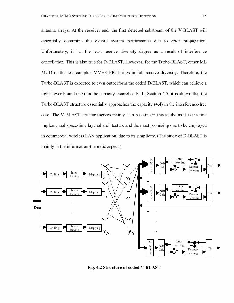
CHAPTER 4. MIMO SYSTEMS: TURBO SPACE-TIME MULTIUSER DETECTION 115
antenna arrays. At the receiver end, the first detected substream of the V-BLAST will
essentially determine the overall system performance due to error propagation.
Unfortunately, it has the least receive diversity degree as a result of interference
cancellation. This is also true for D-BLAST. However, for the Turbo-BLAST, either ML
MUD or the less-complex MMSE PIC brings in full receive diversity. Therefore, the
Turbo-BLAST is expected to even outperform the coded D-BLAST, which can achieve a
tight lower bound (4.5) on the capacity theoretically. In Section 4.5, it is shown that the
Turbo-BLAST structure essentially approaches the capacity (4.4) in the interference-free
case. The V-BLAST structure serves mainly as a baseline in this study, as it is the first
implemented space-time layered architecture and the most promising one to be employed
in commercial wireless LAN application, due to its simplicity. (The study of D-BLAST is
mainly in the information-theoretic aspect.)
Fig. 4.2 Structure of coded V-BLAST
Inter-leaving
Inter-leaving
Inter-leavingCoding Mapping
1xCoding Mapping
Coding MappingCoding Mapping2x
Coding MappingCoding Mapping
Nx
.
.
.
1y
2y
Ny
-
.
.
.
SoftCalc Dec
Inter-leaving
Deinter-leaving- -M
MSE
SoftCalc Dec
Inter-leaving
Deinter-leaving- -M
MSE
SoftCalc Dec
Inter-leaving
Deinter-leaving- -M
MSE
-Inter-
leaving
Inter-leaving
Inter-leavingCoding Mapping
1xCoding Mapping
Coding MappingCoding Mapping2x
Coding MappingCoding Mapping
Nx
.
.
.
1y
2y
Ny
-
.
.
.
SoftCalc Dec
Inter-leaving
Deinter-leaving- -M
MSE
SoftCalc Dec
Inter-leaving
Deinter-leaving- -M
MSE
SoftCalc Dec
Inter-leaving
Deinter-leaving- -M
MSE
SoftCalc Dec
Inter-leaving
Deinter-leaving- -M
MSE
SoftCalc Dec
Inter-leaving
Deinter-leaving- -M
MSE
SoftCalc Dec
Inter-leaving
Deinter-leaving- -M
MSE
-Data
Inter-leaving
Inter-leaving
Inter-leavingCoding Mapping
1x1xCoding Mapping
Coding MappingCoding Mapping2x 2x
Coding MappingCoding Mapping
Nx Nx
.
.
.
1y 1y
2y 2y
Ny Ny
-
.
.
.
SoftCalc Dec
Inter-leaving
Deinter-leaving- -M
MSE
SoftCalc Dec
Inter-leaving
Deinter-leaving- -M
MSE
SoftCalc Dec
Inter-leaving
Deinter-leaving- -M
MSE
SoftCalc Dec
Inter-leaving
Deinter-leaving- -M
MSE
SoftCalc Dec
Inter-leaving
Deinter-leaving- -M
MSE
-Inter-
leaving
Inter-leaving
Inter-leavingCoding Mapping
1x1xCoding Mapping
Coding MappingCoding Mapping2x 2x
Coding MappingCoding Mapping
Nx Nx
.
.
.
1y 1y
2y 2y
Ny Ny
-
.
.
.
SoftCalc Dec
Inter-leaving
Deinter-leaving- -M
MSE
SoftCalc Dec
Inter-leaving
Deinter-leaving- -M
MSE
SoftCalc Dec
Inter-leaving
Deinter-leaving- -M
MSE
SoftCalc Dec
Inter-leaving
Deinter-leaving- -M
MSE
SoftCalc Dec
Inter-leaving
Deinter-leaving- -M
MSE
SoftCalc Dec
Inter-leaving
Deinter-leaving- -M
MSE
-Data

CHAPTER 4. MIMO SYSTEMS: TURBO SPACE-TIME MULTIUSER DETECTION 116
Fig. 4.3 Structure of Turbo-BLAST
4.3.2 Turbo-BLAST Detection The turbo decoding procedure of the coded V-BLAST is exactly analogous to that of the
Turbo-BLAST to be discussed and therefore is omitted here. The Turbo-BLAST
detection algorithm involves two components: demodulation and decoding. The
demodulation stage with ML is straightforward. Suppose an N N× MIMO system is
employed by one cell, and each substream adopts M-QAM (quadrature amplitude
modulation). Then for each symbol interval 2logB N M= ⋅ bits are jointly detected. The
extrinsic information for the kth bit of the ith substream symbol, 21 logk M≤ ≤ ,
1 i N≤ ≤ , is given by
1 , 1 , 2 ,
,
,
( ) ( ) ( )
( | ) ( )( 1)
log log ,( | ) ( ) ( 1)
i
i
pk i k i k i
X k i
k iX
b b b
p pP b
p p P b
λ λ
+
−
∈
∈
= Λ −
== −
= −
∑∑
x
x
y x x
y x x (4.9)
Mapping1x
Mapping
MappingMapping2x
MappingMappingNx
1y
2y
Ny
Mapping1x
Mapping
MappingMapping2x
MappingMappingNx
1y
2y
Ny
Inter-leaving
Coding
BLAST
De-Mapping
(MLor
MMSEPIC)
Dec
Inter-leaving
Deinter-leaving-
Inter-leaving
Deinter-leaving-
-...
Mapping1x1x
Mapping
MappingMapping2x2x
MappingMappingNx Nx
1y1y
2y 2y
Ny Ny
Mapping1x1x
Mapping
MappingMapping2x2x
MappingMappingNx Nx
1y1y
2y 2y
Ny Ny
Inter-leaving
Coding
BLAST
De-Mapping
(MLor
MMSEPIC)
Dec
Inter-leaving
Deinter-leaving-
Inter-leaving
Deinter-leaving-
-... 1 ,( )k ibΛ 1 ,( )k ibλ
2 ,( )pk ibλ
2 ( )jbλ
1 ( )pjbλ
2 ( )jbΛMapping1x1x
Mapping
MappingMapping2x2x
MappingMappingNx Nx
1y1y
2y 2y
Ny Ny
Mapping1x1x
Mapping
MappingMapping2x2x
MappingMappingNx Nx
1y1y
2y 2y
Ny Ny
Inter-leaving
Coding
BLAST
De-Mapping
(MLor
MMSEPIC)
Dec
Inter-leaving
Deinter-leaving-
Inter-leaving
Deinter-leaving-
-...
Mapping1x1x
Mapping
MappingMapping2x2x
MappingMappingNx Nx
1y1y
2y 2y
Ny Ny
Mapping1x1x
Mapping
MappingMapping2x2x
MappingMappingNx Nx
1y1y
2y 2y
Ny Ny
Inter-leaving
Coding
BLAST
De-Mapping
(MLor
MMSEPIC)
Dec
Inter-leaving
Deinter-leaving-
Inter-leaving
Deinter-leaving-
-... 1 ,( )k ibΛ 1 ,( )k ibλ
2 ,( )pk ibλ
2 ( )jbλ
1 ( )pjbλ
2 ( )jbΛ

CHAPTER 4. MIMO SYSTEMS: TURBO SPACE-TIME MULTIUSER DETECTION 117
where 1 2 ,( , , , ) : 1T
i N k iX x x x b+ = =… and 1 2 ,( , , , ) : 1Ti N k iX x x x b− = = −… ; ( | )p y x is a
multivariate Gaussian distribution (see (4.1)); ( )2 , , ,( ) log ( 1) ( 1)pk i k i k ib P b P bλ = = = − and
,,
( ) ( )k ik i
p p b=∏x comprise a priori information from the decoding stage.
The demodulation stage with PIC is subtler. Suppose the received signal for some
substream 1 k N≤ ≤ after interference cancellation is given by
( ) ,k k= − +y H x x n (4.10)
where 1 2( , , 0, , )Tk k Nx x x x= =x … … is the estimated interference vector. First an MMSE
filter is applied to ky to further suppress the residual interference plus noise, that is,
1 * 1[ ] [ ] ( ) ,H H Hk k k k k k k k k k
NE E xρ
− −= = + +w y y y h h H QH I h (4.11)
where kh is the kth column of matrix H, kH is the complement of kh in H, and
2 2 2 21 1 1diag[1 | | , ,1 | | ,1 | | , ,1 | | ]N N N N
k k NP P P Px x x x− += − − − −Q … … , which approaches 0
when estimates from the decoding stage are accurate enough for constant-modulus
signals. As is shown in [80], the output of the MMSE filter Hk k kz = w y can be written as
,k k k kz xµ η= + (4.12)
where *[ ]N Hk k k k kP E z xµ = = w h , and kη is a Gaussian variable with zero mean and
variance 2 2 2 2 2[| | ] [| | ] | | ( | | ).P Pk k k k k k k kN NE z x E zν µ µ µ µ= − = − = − The extrinsic
information is given in the same form as (4.9), but with y replaced by kz and x with kx ,
and (4.1) replaced with (4.12), and therefore with much lower complexity.

CHAPTER 4. MIMO SYSTEMS: TURBO SPACE-TIME MULTIUSER DETECTION 118
For the channel decoding stage let us consider a binary 1/n convolutional code with
constraint length υ (the soft decoding for other codes, e.g., Turbo codes, is similar). The
BCJR decoding algorithm [5] is known to yield the optimal symbol estimate with
minimum symbol-error-rate. What is more important for turbo processing is the BCJR
algorithm’s ability to yield soft information in the form of a posteriori log-likelihood
ratios (LLRs) for coded and information bits. Using the same notation as in [5], for stage
t of the code trellis transiting from state 1tS s− ′= to tS s= associated with input td and
output 1( , , )nt t tb b=b … (where k
j tb b↔ with ( 1)j t n k= − + for a rate-
1/ n convolutional code), we have
1
1
( ) ( , ) ( )( ) log ,
( ) ( , ) ( )k
k
t t tSk
tt t t
S
s s s sb
s s s s
α γ β
α γ β+
−
−
−
′ ′
Λ =′ ′
∑
∑ (4.13)
where kS + is the set of state pairs ( , )s s′ such that the kth coded bit at stage t is 1 and kS −
is the corresponding set for -1; and
1
1
( ) ( , ) ( )( ) log ,
( ) ( , ) ( )k
k
t t tU
tt t t
U
s s s sd
s s s s
α γ β
α γ β+
−
−
−
′ ′
Λ =′ ′
∑
∑ (4.14)
where kU + is the set of state pairs ( , )s s′ such that the information bit at stage t is 1 and
kU − is the corresponding set for -1. The ( )t sα , ( )t sβ and ( , )t s sγ ′ terms are defined as
follows. ( , )t s sγ ′ denotes the transition probability for the branch s s′ → for the stage t of
the code trellis. As no channel outputs are available for the outer code (the convolutional

CHAPTER 4. MIMO SYSTEMS: TURBO SPACE-TIME MULTIUSER DETECTION 119
code is treated as the outer code while the modulation is treated as the inner code for this
concatenated system) of a concatenated coding system, we have
1 11 1
1( , ) ( | ) ( ) [1 tanh( ( ))],2
n nl p
t t t t j jl l
s s P S s S s P b b bγ λ−= =
′ ′= = = = = +∏ ∏ (4.15)
where kj tb b↔ with ( 1)j t n k= − + , and 1 ( )p
jbλ represents the corresponding a
priori LLR delivered from the demodulation stage that is related to the state transition of
s s′ → . The tα and tβ terms are defined with forward and backward recursions as
1( ) ( ) ( , ), 1, 2, , ,t t ts
s s s s tα α γ τ−′
′ ′= =∑ … (4.16)
and
1 1( ) ( ) ( , ), 1, 2, , 0,t t ts
s s s s tβ β γ τ τ+ +′
′ ′= = − −∑ … (4.17)
with boundary conditions
0 0(0) 1, and ( ) 0, for 0,s sα α= = ≠ (4.18)
and
(0) 1, and ( ) 0, for 0,s sτ τβ β= = ≠ (4.19)
where τ denotes the frame length of the information bits. The summations of (4.16) and
(4.17) are over all states s′ for which the transition s s′ ↔ is possible. So the extrinsic
information produced by the SISO channel decoder can be written as
1
1,2 2 1
11,
( ) ( ) ( )( ) log ( ) ( ),
( ) ( ) ( )
k
k
nl
t t tl l kSk k p k
t t tnl
t t tl l kS
s s P bb b b
s s P b
α βλ λ
α β
+
−
−= ≠
−= ≠
′
= = Λ −′
∑ ∏
∑ ∏ (4.20)

CHAPTER 4. MIMO SYSTEMS: TURBO SPACE-TIME MULTIUSER DETECTION 120
where again kj tb b↔ with ( 1)j t n k= − + for a rate-1/ n convolutional code.
The BCJR algorithm is known to have numerical problems associated with the
representations of probabilities due to the large dynamic range of tα and tβ . Thus it is
preferable that operations be processed in the logarithmic domain [90], [123]. With the
substitution of log( )t ta α= , log( )t tb β= and log( )t tc γ= , (4.13) can be rewritten as
1 1( ) log exp( ) log exp( ) ,k k
kt t t t t t t
S S
b a c b a c b+ −
− −
Λ = + + − + +
∑ ∑ (4.21)
where
1
1 1 1
exp( ( ))( , ) log( ( )) log( ),1 exp( ( ))
l p ln nl t t
t t l p ll l t t
b bc s s P bb bλλ= =
′ = =+∑ ∑ (4.22)
1( ) log exp( ( ) ( , )) ,t t ts
a s a s c s s−′
′ ′= + ∑ (4.23)
with
0 0(0) 0, and ( ) , for 0a a s s= = −∞ ≠ , (4.24)
and
1 1( ) log exp( ( ) ( , )) ,t t ts
b s b s c s s+ +′
′ ′= + ∑ (4.25)
with
(0) 0, and ( ) , for 0b b s sτ τ= = −∞ ≠ . (4.26)
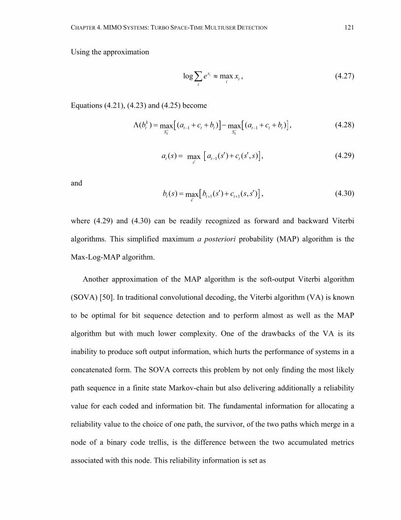
CHAPTER 4. MIMO SYSTEMS: TURBO SPACE-TIME MULTIUSER DETECTION 121
Using the approximation
log maxixiii
e x≈∑ , (4.27)
Equations (4.21), (4.23) and (4.25) become
[ ] [ ]1 1( ) ( ) ( ) ,max maxk k
kt t t t t t t
S Sb a c b a c b
+ −− −Λ = + + − + + (4.28)
[ ]1( ) ( ) ( , ) ,maxt t ts
a s a s c s s−′
′ ′= + (4.29)
and [ ]1 1( ) ( ) ( , )maxt t t
sb s b s c s s+ +
′′ ′= + , (4.30)
where (4.29) and (4.30) can be readily recognized as forward and backward Viterbi
algorithms. This simplified maximum a posteriori probability (MAP) algorithm is the
Max-Log-MAP algorithm.
Another approximation of the MAP algorithm is the soft-output Viterbi algorithm
(SOVA) [50]. In traditional convolutional decoding, the Viterbi algorithm (VA) is known
to be optimal for bit sequence detection and to perform almost as well as the MAP
algorithm but with much lower complexity. One of the drawbacks of the VA is its
inability to produce soft output information, which hurts the performance of systems in a
concatenated form. The SOVA corrects this problem by not only finding the most likely
path sequence in a finite state Markov-chain but also delivering additionally a reliability
value for each coded and information bit. The fundamental information for allocating a
reliability value to the choice of one path, the survivor, of the two paths which merge in a
node of a binary code trellis, is the difference between the two accumulated metrics
associated with this node. This reliability information is set as

CHAPTER 4. MIMO SYSTEMS: TURBO SPACE-TIME MULTIUSER DETECTION 122
[ ] [ ]2 1 1 1( ) ( ) ( ) ( , ) ( ) ( , ) ,max mint t t t tss
M t M t a s c s s a s c s s− −′′
′ ′ ′ ′∆ = − = + − + (4.31)
for some node s of the maximum likelihood sequence at time t, where 2 ( )M t denotes the
accumulated metric to time t of the survivor path while 1( )M t denotes that of the
discarded path. The probability that we make the correct choice is given by
2
1 2(correct)1
t
t
M
M Me eP
e e e
∆
∆= =+ +
. (4.32)
So,
( )log1 ( )t
P correctP correct
∆ =−
(4.33)
is just the LLR for this binary path decision. Suppose we want to obtain soft output for a
coded bit ktb , which the SOVA decides after a delay of δ . Then on the section of the
maximum likelihood path from stage t to t δ+ , 1δ + nonsurviving paths , ,n nt t δ+s s… have
been discarded. Let us denote the soft information along this section of the ML path by
, ,t t δ+∆ ∆… , and examine for each nonsurviving path whether ˆ ( )k k nt t t lb b +≠ , where ˆk
tb is
the ML estimate, and ( )k nt t lb + is the associated kth bit at time t for the nonsurviving path
nt l+s , 0 l δ≤ ≤ . Then the SOVA-based LLR for k
tb is approximately given by
20
ˆ( ) ,mink kt t t l
lb b
δ+
≤ ≤Λ ≅ ⋅ ∆ (4.34)
where the minimum is taken over only those nonsurviving paths which would have a
different estimate for ktb . Similar results can be obtained for the LLRs of the information
bits. Note that we have assumed the ML path has already been obtained before tracing

CHAPTER 4. MIMO SYSTEMS: TURBO SPACE-TIME MULTIUSER DETECTION 123
back to decide the LLR value. Modification of this procedure for truncated ML path
selection is straightforward.
Now that we have described the three most commonly used SISO decoding
algorithms, we would like to make a brief comparison between them. The MAP
algorithm takes account of all the paths in the trellis and divides them into two sets (see
(124)), corresponding to the specific binary value of the bit of interest. This division
varies from stage by stage. In contrast, the Max-Log-MAP considers only two paths, the
ML path and another closest path to the ML path differing only at the transition
associated with the bit of interest (see (4.28)). Thus, Max-Log-MAP is suboptimal with
respect to MAP with simplified metric computation. However, the loss due to this
suboptimality is typically within 0.5 dB for AWGN channels and is negligible for
realistic channels, because the Max-Log-MAP algorithm is more robust when the system
has estimation errors or the noise is not strictly Gaussian [68]. Furthermore, by replacing
logarithms by Jacobian logarithms, defined as
1 2 2 1| |1 2log( ) max( , ) log(1 ),x x x xe e x x e− −+ = + + (4.35)
Max-Log-MAP can be transformed back to exact MAP. Compared to (25), this change
requires the addition of only one correction term, which can easily be implemented with a
one-dimensional lookup table [90]. Compared to Max-Log-MAP, SOVA also deals with
only two paths: one is the ML path, but the other is not necessarily the same as that
considered in Max-Log-MAP, the best competing path. Thus, SOVA will lose
approximately another 0.5 dB in performance compared with Max-Log-MAP, but with a
much lower complexity [68]. Again, it is shown in [44] that some modifications can be
made on SOVA to make it equivalent to Max-Log-MAP.

CHAPTER 4. MIMO SYSTEMS: TURBO SPACE-TIME MULTIUSER DETECTION 124
4.4 Multiuser Detection to Combat Intercell Interference We have already discussed various MUD schemes for detection of different substreams
within a MIMO system (intracell interference). Here we will focus on exploiting MUD to
combat interference of the same format from adjacent cells (intercell interference).
4.4.1 Maximum Likelihood MUD Maximum likelihood multiuser detection is infeasible for most current applications due to
its complexity. Suppose an N N× MIMO system is employed by one cell, and each
substream adopts M-QAM. Then the ML-MUD complexity would be in the order of
NM . If we want to jointly detect all the information bits for users from desired and K-1
interfering cells, then the complexity would go to the order of NKM . Even if we assume
the simplest scheme such as 4M = , 2N = and 5K = (ignoring the two weakest
interfering cells of the first tier), the complexity would be in the order of 202 , which is
beyond the capacity of all current practical systems.
4.4.2 Linear MMSE MUD We assume knowledge of channel information for the interfering users, which can be
obtained either through a joint training phase with the coordination of base stations, or
through adaptive tracking algorithms from the received signals directly. MMSE MUD,
which is generally the most favorable linear MUD, has a detection matrix given by (c.f.
(4.8))
1
.ifiH Hifi ifi
i
P NP ρ
−
= + +
∑W HH H H I H (4.36)
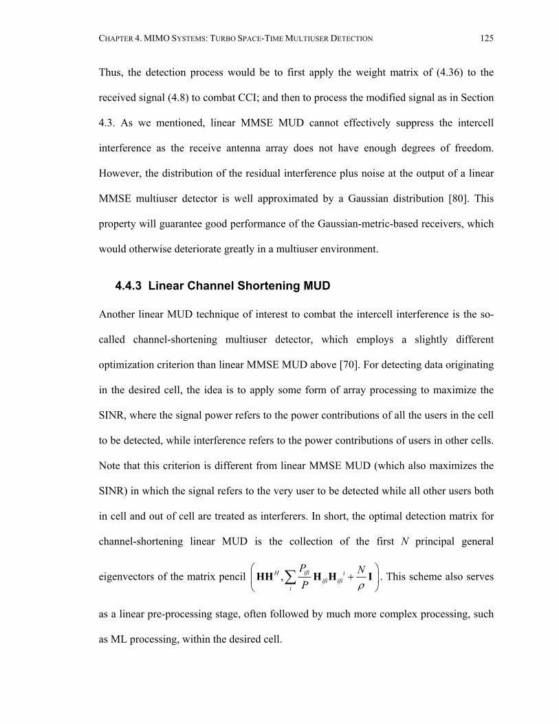
CHAPTER 4. MIMO SYSTEMS: TURBO SPACE-TIME MULTIUSER DETECTION 125
Thus, the detection process would be to first apply the weight matrix of (4.36) to the
received signal (4.8) to combat CCI; and then to process the modified signal as in Section
4.3. As we mentioned, linear MMSE MUD cannot effectively suppress the intercell
interference as the receive antenna array does not have enough degrees of freedom.
However, the distribution of the residual interference plus noise at the output of a linear
MMSE multiuser detector is well approximated by a Gaussian distribution [80]. This
property will guarantee good performance of the Gaussian-metric-based receivers, which
would otherwise deteriorate greatly in a multiuser environment.
4.4.3 Linear Channel Shortening MUD Another linear MUD technique of interest to combat the intercell interference is the so-
called channel-shortening multiuser detector, which employs a slightly different
optimization criterion than linear MMSE MUD above [70]. For detecting data originating
in the desired cell, the idea is to apply some form of array processing to maximize the
SINR, where the signal power refers to the power contributions of all the users in the cell
to be detected, while interference refers to the power contributions of users in other cells.
Note that this criterion is different from linear MMSE MUD (which also maximizes the
SINR) in which the signal refers to the very user to be detected while all other users both
in cell and out of cell are treated as interferers. In short, the optimal detection matrix for
channel-shortening linear MUD is the collection of the first N principal general
eigenvectors of the matrix pencil , ifiH iifi ifi
i
P NP ρ
+
∑HH H H I . This scheme also serves
as a linear pre-processing stage, often followed by much more complex processing, such
as ML processing, within the desired cell.
CHAPTER 4. MIMO SYSTEMS: TURBO SPACE-TIME MULTIUSER DETECTION 126
4.4.4 Group IC MUD Since ML-MUD is highly complex, while linear MUD is limited in its interference
cancellation capability (especially for heavy-loaded systems), non-linear MUD often
provides a tradeoff between performance and complexity, as noted in Chapter 3. In the
context of multicell MIMO systems, group detection techniques naturally call for
attention, in which information bits for one group (one cell MIMO) are detected at a time.
Following a natural extension from BLAST, we can detect one MIMO system at a time,
and feed decisions to other group detectors for interference cancellation. Successive
interference cancellation, even though far from the optimum detection scheme, is
nonetheless asymptotically optimal under the assumption of perfect interference
cancellation [117]. Note that in practice, the success of interference cancellation relies on
the correct detection of interference. In adverse environments where we cannot get good
estimates of interference, IC schemes will worsen the performance instead of improving
it. The potential benefit of group IC MUD depends highly on the interference structure,
which will be addressed further in the next section.
4.5 Numerical Results
4.5.1 Comparison of Various MUD Schemes for Intercell Interference Mitigation
In Section 4.3 and 4.4, various potential advanced techniques have been introduced, the
combination of which could yield many detector structures. We now compare them,
based on the model (4.8), to see which one performs best in the interference-limited
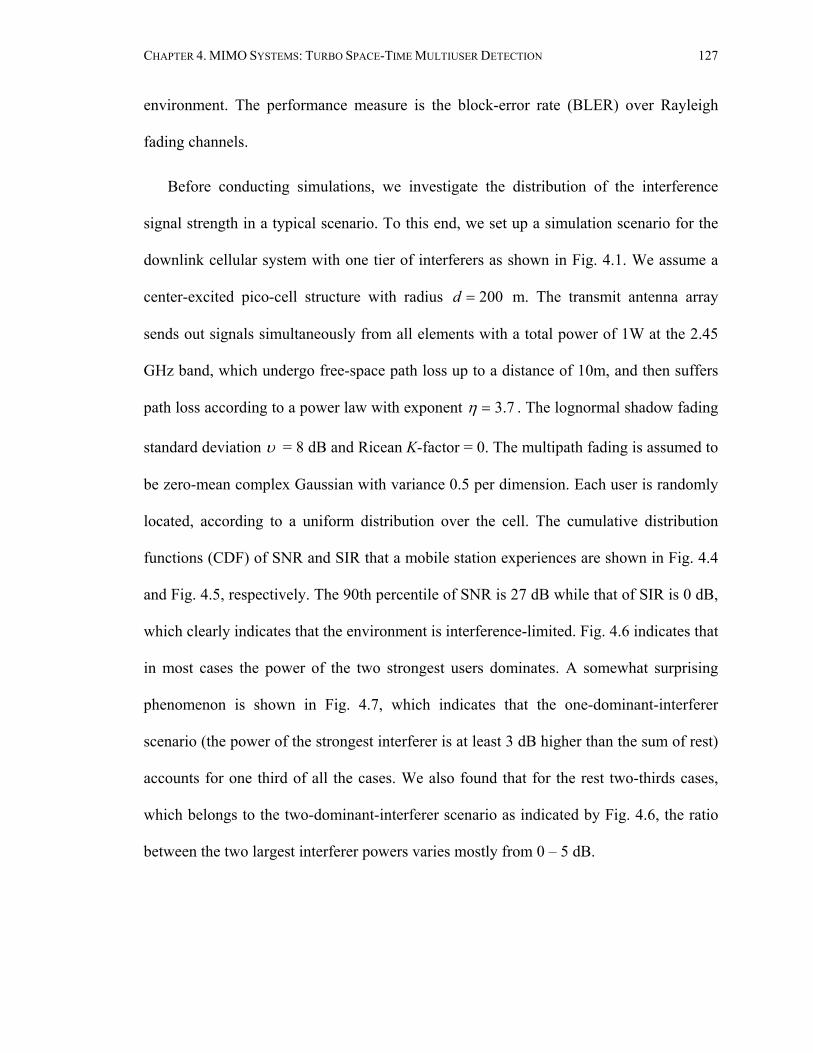
CHAPTER 4. MIMO SYSTEMS: TURBO SPACE-TIME MULTIUSER DETECTION 127
environment. The performance measure is the block-error rate (BLER) over Rayleigh
fading channels.
Before conducting simulations, we investigate the distribution of the interference
signal strength in a typical scenario. To this end, we set up a simulation scenario for the
downlink cellular system with one tier of interferers as shown in Fig. 4.1. We assume a
center-excited pico-cell structure with radius 200=d m. The transmit antenna array
sends out signals simultaneously from all elements with a total power of 1W at the 2.45
GHz band, which undergo free-space path loss up to a distance of 10m, and then suffers
path loss according to a power law with exponent 7.3=η . The lognormal shadow fading
standard deviation υ = 8 dB and Ricean K-factor = 0. The multipath fading is assumed to
be zero-mean complex Gaussian with variance 0.5 per dimension. Each user is randomly
located, according to a uniform distribution over the cell. The cumulative distribution
functions (CDF) of SNR and SIR that a mobile station experiences are shown in Fig. 4.4
and Fig. 4.5, respectively. The 90th percentile of SNR is 27 dB while that of SIR is 0 dB,
which clearly indicates that the environment is interference-limited. Fig. 4.6 indicates that
in most cases the power of the two strongest users dominates. A somewhat surprising
phenomenon is shown in Fig. 4.7, which indicates that the one-dominant-interferer
scenario (the power of the strongest interferer is at least 3 dB higher than the sum of rest)
accounts for one third of all the cases. We also found that for the rest two-thirds cases,
which belongs to the two-dominant-interferer scenario as indicated by Fig. 4.6, the ratio
between the two largest interferer powers varies mostly from 0 – 5 dB.

CHAPTER 4. MIMO SYSTEMS: TURBO SPACE-TIME MULTIUSER DETECTION 128
10 20 30 40 50 60 70 80 90 1000
10
20
30
40
50
60
70
80
90
100CDF of SNR
SNR (dB)
F(x)
Fig. 4.4 CDF of SNR experienced by a mobile
-10 0 10 20 30 40 50 60 700
10
20
30
40
50
60
70
80
90
100CDF of SIR
SIR (dB)
F(x)
Fig. 4.5 CDF of SIR experienced by a mobile

CHAPTER 4. MIMO SYSTEMS: TURBO SPACE-TIME MULTIUSER DETECTION 129
-5 0 5 10 15 20 25 30 350
10
20
30
40
50
60
70
80
90
100CDF of Ratio2
Ratio2 (dB)
F(x)
Fig. 4.6 CDF of the ratio between the power sum of the two strongest interferers and
the power sum of the remaining interferers experienced by a mobile
-10 -5 0 5 10 15 20 25 300
10
20
30
40
50
60
70
80
90
100CDF of Ratio1
Ratio1 (dB)
F(x)
Fig. 4.7 CDF of the ratio between the power of the strongest interferer and the
power sum of the remaining interferers experienced by a mobile

CHAPTER 4. MIMO SYSTEMS: TURBO SPACE-TIME MULTIUSER DETECTION 130
We assume that each cell employs a 4 4× MIMO system, operating at SNR = 30 dB.
The modulation scheme employed is 4QAM. The coding scheme used is a rate-1/3 64-
state convolutional code with generators 1 2 3 8( , , ) (155,117,123)G G G = (as proposed for
EDGE). It was shown in our simulations that this code achieves better performance than
a turbo-code with two identical 16-state recursive encoders with generators
1 2 8( , ) (23,31)G G = , at a considerably lower complexity. We transmit blocks of 384
information bits, and record the block error probability of this system.
The receiver structure is either V-BLAST or Turbo-BLAST, combined with various
MUD schemes. To be specific, the receivers we study are: 1) Coded V-BLAST (V-
BLAST); 2) Coded V-BLAST with linear MMSE MUD pre-processing (V-
BLAST+MMSE); 3) Turbo-BLAST with a parallel interference cancellation
demodulation stage (T-BLAST (PIC)); 4) Turbo-BLAST with a parallel interference
cancellation demodulation stage, with linear MMSE MUD pre-processing (T-BLAST
(PIC)+MMSE); 5) Turbo-BLAST with a maximum likelihood demodulation stage (T-
BLAST (ML)); 6) Turbo-BLAST with a maximum likelihood demodulation stage, with
linear channel shortening MUD pre-processing (T-BLAST (ML)+CS); 7) Turbo-BLAST
with a parallel interference cancellation demodulation stage, with full group IC MUD2
(T-BLAST (PIC)+IC). We study the performance of these receivers in the framework of
(4.8) in two situations: (A) 1 2 3 44 4if if if ifP P P P= = = and (B) 1 2 3 46 6 6if if if ifP P P P= = = .
4321 666 ifififif PPPP === . Situation (A) corresponds to a two-equal-power-dominant-
interferer scenario, while situation (B) reflects a one-dominant-interferer case.
2 This receiver attempts to detect all the interfering signals of interest
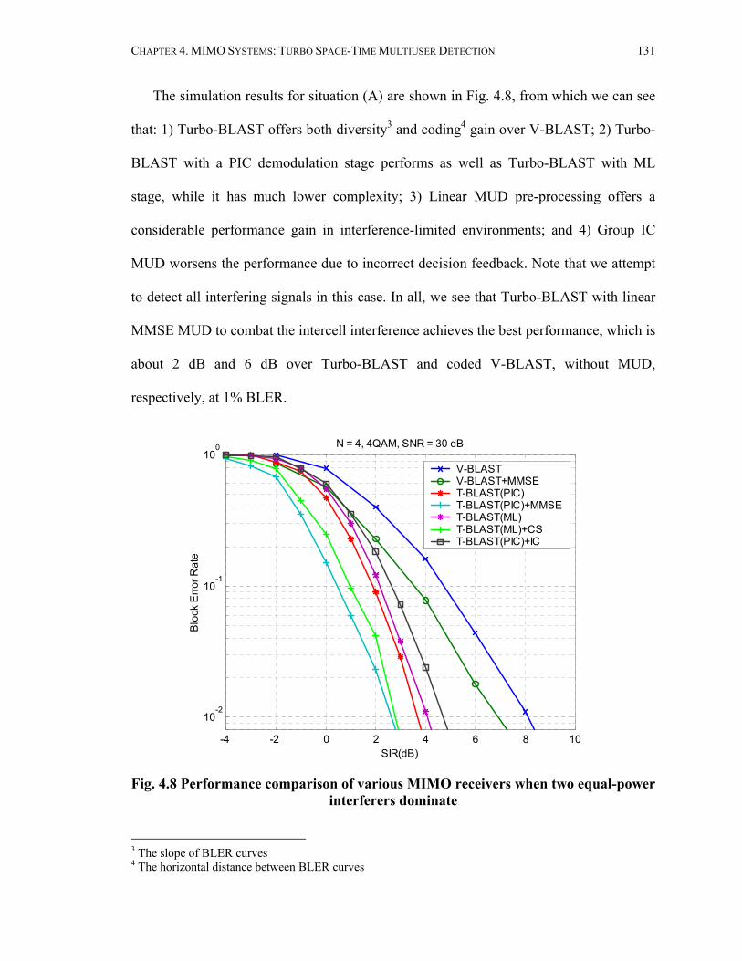
CHAPTER 4. MIMO SYSTEMS: TURBO SPACE-TIME MULTIUSER DETECTION 131
The simulation results for situation (A) are shown in Fig. 4.8, from which we can see
that: 1) Turbo-BLAST offers both diversity3 and coding4 gain over V-BLAST; 2) Turbo-
BLAST with a PIC demodulation stage performs as well as Turbo-BLAST with ML
stage, while it has much lower complexity; 3) Linear MUD pre-processing offers a
considerable performance gain in interference-limited environments; and 4) Group IC
MUD worsens the performance due to incorrect decision feedback. Note that we attempt
to detect all interfering signals in this case. In all, we see that Turbo-BLAST with linear
MMSE MUD to combat the intercell interference achieves the best performance, which is
about 2 dB and 6 dB over Turbo-BLAST and coded V-BLAST, without MUD,
respectively, at 1% BLER.
-4 -2 0 2 4 6 8 10
10-2
10-1
100 N = 4, 4QAM, SNR = 30 dB
SIR(dB)
Blo
ck E
rror R
ate
V-BLAST V-BLAST+MMSE T-BLAST(PIC) T-BLAST(PIC)+MMSET-BLAST(ML) T-BLAST(ML)+CS T-BLAST(PIC)+IC
Fig. 4.8 Performance comparison of various MIMO receivers when two equal-power
interferers dominate
3 The slope of BLER curves 4 The horizontal distance between BLER curves

CHAPTER 4. MIMO SYSTEMS: TURBO SPACE-TIME MULTIUSER DETECTION 132
The failure of group IC MUD is owing to the inability to correctly detect the
information bits for interfering cells. There are both theoretical and practical reasons for
the errors in the detection of the interfering signals. The practical reason is that the codes
that we used in this simulation are comparatively simple, and thus cannot correct all the
errors that an “ideal” code could eliminate. However, there is also a theoretical limit: with
ideal codes, the codes in neighboring cells would be designed to have rates that achieve
capacity in that cell. However, they suffer more attenuation when propagating to the
neighboring cell (where they are interferers). The signal-to-noise-ratios of those signals in
the neighboring cells are thus worse, so that the data rate is above the capacity of the link
to the neighboring cell. Thus, correct decisions for the symbols of interfering signals
might not be possible even theoretically.
Decoding of the data for interfering cells is done with the hope that this can aid in
detecting the data for the desired cell. Otherwise, it is a waste of resource to do this.
Moreover, wrong decision feedback can interfere with the iterative processing of the
desired user, and actually worsens the performance. Thus, instead of decoding the data
for all interfering cells, it makes sense to do it for just one or two strongest interfering
signals and to ignore the others. The simulation results in Fig. 4.9 indicate the
effectiveness of this approach. However, the performance of group IC MUD is still worse
than linear MMSE.
We would expect that when we have only one dominant interfering signal, group IC
MUD will outperform linear MMSE MUD. Therefore, it is worth studying the
performance of group IC MUD only for the strongest interfering signal when there is one
dominant interferer. The simulation results for situation (B) are shown in Fig. 4.10. We

CHAPTER 4. MIMO SYSTEMS: TURBO SPACE-TIME MULTIUSER DETECTION 133
-4 -3 -2 -1 0 1 2 3 4 5
10-2
10-1
100 N = 4, 4QAM, SNR = 30dB
SIR(dB)
Blo
ck E
rror R
ate
T-BLAST(PIC)+FULL ICT-BLAST(PIC)+2 IC T-BLAST(PIC)+1 IC T-BLAST(PIC)+MMSE
Fig. 4.9 Performance comparison of various versions of group IC MUD when two
equal-power interferers dominate
-8 -6 -4 -2 0 2 4 6 8 10 12 14
10-2
10-1
100 N = 4, 4QAM, SNR = 30 dB
SIR(dB)
Blo
ck E
rror R
ate
V-BLAST V-BLAST+MMSE T-BLAST(PIC) T-BLAST(PIC)+MMSET-BLAST+FULL IC T-BLAST(PIC)+2 ICT-BLAST(PIC)+1 IC
Fig. 4.10 Performance comparison of various MIMO receivers when one interferer
dominates

CHAPTER 4. MIMO SYSTEMS: TURBO SPACE-TIME MULTIUSER DETECTION 134
see that group IC MUD only for the strongest interfering signal achieves the best
performance, which is about 4 dB and 8 dB over Turbo-BLAST and coded V-BLAST,
without MUD, respectively, and more than 2 dB over Turbo-BLAST with linear MMSE
preprocessing, at 1% BLER. (Since T-BLAST (ML) assumes no advantage over T-
BLAST (PIC) while having much higher complexity, we do not consider it further.)
We have noticed that group IC MUD performs the best when one interferer
dominates. But when two interferers dominate that have the same power, it is no better
than the simpler linear MMSE scheme. Figures 4.11 to 4.13 show that in the two-
dominant-interferer scenario, when the ratio between the two largest interferer powers
increases, the gap between the performance of group IC MUD and linear MMSE MUD
also increases. In the view of this performance, an idea for adaptive detection arises:
namely, in the case of one dominant interferer (3 dB or greater) or in the case of two
dominant interferers (4 dB or greater) with the ratio between the two largest interferer
power greater than 3 dB, group IC MUD could be adopted, otherwise the simple MMSE
scheme could be adopted. Please note that the adaptive scheme proposed here is well
suited for the corresponding setting. It should be modified when applying to other
scenarios, even though the adaptive detection idea is carried on readily.
4.5.2 Downlink Capacity of Interference-Limited MIMO
Figures 4.14 and 4.15 give the outage capacity for interference limited MIMO when one
and two interferers with equal power dominate, respectively. An upper bound
(corresponding to the no-interference situation) is derived from (4.4), where the block
error rate is defined as the probability that the specified spectral efficiency (8/3 bits/s/Hz

CHAPTER 4. MIMO SYSTEMS: TURBO SPACE-TIME MULTIUSER DETECTION 135
for 1/3 coded 4QAM-modulated 44 × MIMO system) is not supported by the randomly
generated channels. The Foschini approximation (single link capacity lower bound) is
similarly derived from (4.5). For the one-dominant-interferer case, Turbo-BLAST with a
parallel interference cancellation demodulation stage, with one group IC MUD (T-
BLAST (PIC)+1 IC) is employed, while for the two-equal-power-dominant-interferer
case, Turbo-BLAST with a parallel interference cancellation demodulation stage and
with linear MMSE MUD pre-processing (T-BLAST (PIC)+MMSE) is used, as they
achieve the best performance in each respective case.
-4 -3 -2 -1 0 1 2 3 4
10-2
10-1
100 N = 4, 4QAM, SNR = 30dB
SIR (dB)
Blo
ck E
rror R
ate
T-BLAST(PIC)+2 ICT-BLAST(PIC)+1 ICT-BLAST(PIC)+MMSE
Fig. 4.11 Performance comparison of linear MMSE and group IC MUD when two
interferers dominate with power ratio of 1 dB
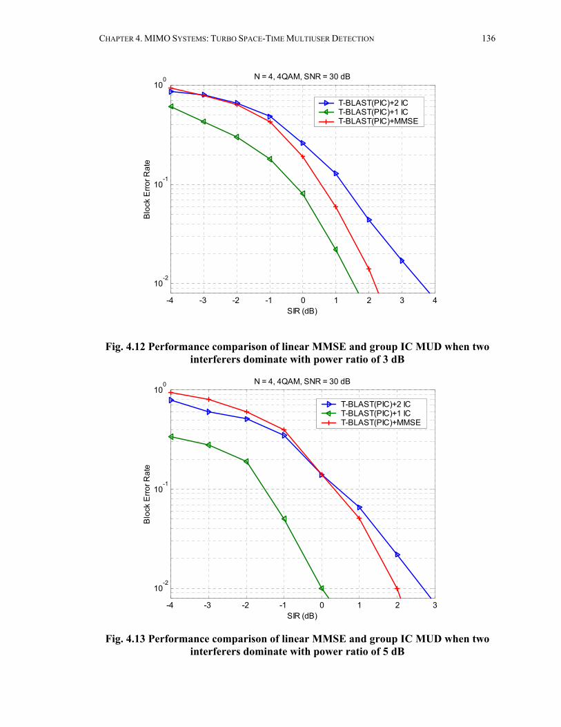
CHAPTER 4. MIMO SYSTEMS: TURBO SPACE-TIME MULTIUSER DETECTION 136
-4 -3 -2 -1 0 1 2 3 4
10-2
10-1
100 N = 4, 4QAM, SNR = 30 dB
SIR (dB)
Blo
ck E
rror R
ate
T-BLAST(PIC)+2 ICT-BLAST(PIC)+1 ICT-BLAST(PIC)+MMSE
Fig. 4.12 Performance comparison of linear MMSE and group IC MUD when two interferers dominate with power ratio of 3 dB
-4 -3 -2 -1 0 1 2 3
10-2
10-1
100 N = 4, 4QAM, SNR = 30 dB
SIR (dB)
Blo
ck E
rror R
ate
T-BLAST(PIC)+2 ICT-BLAST(PIC)+1 ICT-BLAST(PIC)+MMSE
Fig. 4.13 Performance comparison of linear MMSE and group IC MUD when two
interferers dominate with power ratio of 5 dB

CHAPTER 4. MIMO SYSTEMS: TURBO SPACE-TIME MULTIUSER DETECTION 137
The results are given for five situations: interference-free, SIR = 20, 10, 5 and 0 dB.
We see that in the noise-dominating scenario (interference-free, SIR = 20 dB), the MUD
capacity is excellent, even better than the Foschini approximation (Turbo-BLAST usually
yields better performance than D-BLAST). Even when the SIR = 10 dB, the MUD
capacity is quite close to the Foschini approximation, which is only 2-3 dB away from the
exact interference-free capacity. However, when the interference gets stronger, the MUD
capacity gets worse, and eventually saturates, which indicates the limitations of this
method in strong interference environments and leaves ample room for possible
improvement through other techniques. Note that the error floor values of Fig. 4.14 and
Fig. 4.15 when SIR = 0 dB agree well with Fig. 4.10 and Fig. 4.8.
-5 0 5 10 15 20 25 30
10-2
10-1
100 N = 4, 4QAM
SNR (dB)
Blo
ck E
rror R
ate
T-BLAST(PIC)+1 IC SIR=0dB T-BLAST(PIC)+1 IC SIR=5dB T-BLAST(PIC)+1 IC SIR=10dBT-BLAST(PIC)+1 IC SIR=20dBT-BLAST(PIC)+1 IC No Int. single link Capacity LB single link Capacity
Fig. 4.14 Downlink capacity of interference-limited MIMO when one interferer
dominates

CHAPTER 4. MIMO SYSTEMS: TURBO SPACE-TIME MULTIUSER DETECTION 138
-5 0 5 10 15 20 25 30
10-2
10-1
100 N = 4, 4QAM
SNR (dB)
Blo
ck E
rror R
ate
T-BLAST(PIC)+MMSE SIR=0dB T-BLAST(PIC)+MMSE SIR=5dB T-BLAST(PIC)+MMSE SIR=10dBT-BLAST(PIC)+MMSE SIR=20dBT-BLAST(PIC)+MMSE No Int. single link Capacity LB single link Capacity
Fig. 4.15 Downlink capacity of interference-limited MIMO when two interferers
dominate
-5 0 5 10 15 20 25 30
10-2
10-1
100 N = 4, 4QAM
SNR (dB)
Blo
ck E
rror R
ate
SIR=0dB SIM SIR=0dB UB SIR=5dB SIM SIR=5dB UB SIR=10dB SIMSIR=10dB UB SIR=20dB SIMSIR=20dB UB
Fig. 4.16 Comparison of theoretical and simulated results of the capacity of
interference-limited MIMO Systems with linear MMSE front end

CHAPTER 4. MIMO SYSTEMS: TURBO SPACE-TIME MULTIUSER DETECTION 139
In 5.3.3, it is proved that asymptotically (in the large dimensional system sense), the
capacity of interference-limited MIMO systems with the linear MMSE preprocessing is
given by
1logdet[ ( ) ]ifiH HM mmse ifi ifi
i
P NCP ρ
−− = + +∑I HH H H I . (4.37)
In Fig. 4.16, theoretical results of (4.37) are compared with the simulated results for the
two-equal-power-dominant-interferer case (c.f. Fig. 4.15). We see that the simulated
results are only 2 to 3 dB away from the capacity bound for SIR = 20~5 dB at 1% BLER,
and both results exhibit the interference-limited behavior for SIR = 0 dB. The possible
reasons for the gap include: 1) Our simulated system is not a large system ( 44 × MIMO
system); 2) Our Turbo-BLAST structure with the practical convolutional coding already
suffers 1 to 2 dB loss in the interference-free scenario (c.f. Fig. 4.14 and Fig. 4.15).
Therefore, the validity of our simulation results is verified.
4.5.3 Large-Scale Simulation Results So far, the performance evaluations have been done in the framework of (4.8), where we
deliberately set the SNR, SIR, and power distributions among the interferers to fixed
values that represent some typical cases. In this subsection, we test the performance in the
more complete model of (4.7). The receivers of interest are 1) Coded V-BLAST treating
intercell interference as noise (V-BLAST), which serves as a baseline reference; 2)
Turbo-BLAST with a parallel interference cancellation demodulation stage, with linear
MMSE MUD (T-BLAST (PIC)+MMSE); 3) Turbo-BLAST with a parallel interference
cancellation demodulation stage, with adaptive MUD detection (T-BLAST

CHAPTER 4. MIMO SYSTEMS: TURBO SPACE-TIME MULTIUSER DETECTION 140
(PIC)+ADPT); 4) Turbo-BLAST with a parallel interference cancellation demodulation
stage, with the better between linear MMSE and Group IC MUD detection (T-BLAST
(PIC)+IDEAL).
We again assume a 4QAM-modulated 4 4× MIMO system, with the mobile user
randomly located within the cell of interest with the uniform distribution. The figure of
merit is the CDF of the BLER performance for these four receivers. We collect 1000
points for this CDF profile.
4.5.3.1 NLOS Scenario
10-2
10-1
100
30
40
50
60
70
80
90
100CDF of BLER
Block Error Rate
F(x)
V-BLAST T-BLAST(PIC)+MMSE T-BLAST(PIC)+IDEALT-BLAST(PIC)+ADPT
Fig. 4.17 CDF of block error rate for different receivers experienced by a mobile in
Rayleigh fading
The parameters are set as in 4.5.1. The simulation results are shown in Fig. 4.17, from
which we can see that 1) advanced signal processing and coding techniques substantially

CHAPTER 4. MIMO SYSTEMS: TURBO SPACE-TIME MULTIUSER DETECTION 141
improve the performance over the well-known V-BLAST technique with coding (roughly
30% more at 1% outage for the linear MMSE); 2) the adaptive scheme affords further
gain over linear MMSE MUD (roughly 9% more at 1% outage for the ideal case); 3) the
adaptive detection scheme illustrated in 4.5.1 approaches the ideal performance at the low
BER range, which is of practical interest. Note that the threshold values of the adaptive
detection scheme could be refined to get better performance in practice.
4.5.3.2 LOS Scenario A user is randomly located as before, and the probability for LOS decreases linearly with
its distance to a base station, until a "cutoff point", which is set at 300m [103]. If the
signal from some base station is NLOS, the same parameters as 4.5.1 is used. Otherwise,
we set the Ricean factor to
13 0.03K d= − dB, (4.38)
where d is the distance to some base station, and the pathloss exponent to 2. Slightly
different from model (4.6), we assume no shadowing for the LOS component.
Furthermore, we assume that the transmitter and receiver are positioned far apart from
each other compared with the antenna spacing, so we get a rank 1 system matrix for the
LOS component with energy equally distributed between real and imaginary parts [33].
The simulation results are shown in Fig. 4.18. Compared with Fig. 4.17, we see that
the performance of the V-BLAST technique with coding significantly increases due to
less signal fading [63]. MUD techniques with the Turbo-BLAST structure still greatly
improve the system performance over the V-BLAST. But the advantage of the adaptive
scheme over the linear MMSE is negligible.

CHAPTER 4. MIMO SYSTEMS: TURBO SPACE-TIME MULTIUSER DETECTION 142
10-2
10-1
100
30
40
50
60
70
80
90
100CDF of BLER - Ricean
Block Error Rate
F(x)
V-BLAST T-BLAST(PIC)+MMSE T-BLAST(PIC)+IDEALT-BLAST(PIC)+ADPT
Fig. 4.18 CDF of block error rate for different receivers experienced by a mobile in
Ricean fading
4.6 Summary
This chapter has explored the downlink capacity of interference-limited MIMO cellular
fading systems in fading channels. In contrast to the single-cell MIMO system
considered in previous studies, where the intercell interference, when accounted for, is
added to ambient Gaussian noise, we take the approach of modeling the whole downlink
cellular system as a broadcast/interference channel [9], the capacity of which has long
been an open question. As block fading is assumed, we are interested in outage capacity
instead of the Shannon ergodic capacity. Upper bounds for this capacity are obtained
from the interference-free single-link theoretical formulas. We have primarily addressed
the issue of how closely we can approach those bounds without any base station
CHAPTER 4. MIMO SYSTEMS: TURBO SPACE-TIME MULTIUSER DETECTION 143
cooperation by implementation and simulation of advanced techniques. After discussing
the merit of the space-time layered architecture and turbo coding/processing techniques,
which come remarkably close to the ultimate capacity limits with the Gaussian ambient
noise, we have considered multiuser detection for combating intercell interference.
Among various multiuser detection techniques examined, linear MMSE MUD and
successive interference cancellation have been shown to be feasible and effective.
Successive cancellation plays a major role in network information theory from both
theoretical and practical points of view. As is known, decoding of the interfering users is
not always optimal except in the strong-interference case, nor is treating them as pure
ambient noise optimal, except in the very-weak interference case. Based on these
phenomena, we have proposed an adaptive detection idea that offers improved
performance.
The success of linear MMSE processing arises, in addition to its ability to suppress
interference, from its ability of producing Gaussian-like interference [80]. The
observations made in [65] indicate that a receiver that uses a Gaussian-based optimal
metric (which is true for our study) cannot surpass the Gaussian capacity region in the
case of an ergodic additive non-Gaussian channel when Gaussian distributed codewords
are selected. On the other hand, transforming the non-Gaussian interference into
Gaussian-like interference guarantees the excellent performance of efficient signaling
techniques well studied for AWGN channels [12], [39].
We have shown through simulation that advanced signal processing and coding
techniques substantially improve the interference-limited MIMO system performance
over the well-known V-BLAST techniques with coding (6-8 dB in SIR for the simplified

CHAPTER 4. MIMO SYSTEMS: TURBO SPACE-TIME MULTIUSER DETECTION 144
model, or 40% more in capacity for the cellular model, at 1% outage). We have also
shown that the obtained MUD capacity is excellent in high to medium SIR environments.
For the linear MMSE MUD preprocessing, our simulation results have been compared
with the theoretic asymptotic capacity and their validity is verified. Our proposed
techniques might be rather complex for the current systems, but will become more
practically relevant in the future, as computing power at the mobile increases according
to the Moore’s law. Furthermore, they are readily applicable to the base stations for
uplink processing.
Finally, numerical results indicate that, due to complexity constraints and adverse
environments, there is a significant performance gap between MUD capacity and
interference-free capacity, especially in environments with strong interference (SIR of 5
dB or less). This indicates a need to exploit more complex schemes, such as base station
cooperation (macrodiversity) for interference reduction, to enhance the system
throughput.

145
Chapter 5
Spectral Efficiency of Multicell MIMO Systems
5.1 Introduction Recall from Chapter 4 that a recent study by Catreux, Driessen and Greenstein [14]
indicated the ineffectiveness of a MIMO system in an interference-limited environment.
This seems to be related to an insufficient number of degrees of freedom (number of
receive antennas) of the MIMO system to suppress the co-channel interference in contrast
to the smart antenna system, where there is only one transmitted data stream in the
desired cell. On the other hand, this investigation assumed a certain system structure
(uncoded V-BLAST) taken from the noise-limited case, and did not try to optimize the
system for interference-limited environments. Motivated by this study, we restored much
of the performance of the MIMO system (to its promise in a single cell with Gaussian
ambient noise) in a multi-cell structure, through application of advanced signal
processing techniques. We employed a turbo space-time multiuser receiver structure for
intracell communication, which essentially approaches the Shannon limit (within 1-2 dB)
for an isolated cell. Furthermore, we employed another level of multiuser detection to
combat the intercell interference. Among various multiuser detection techniques

CHAPTER 5. SPECTRAL EFFICIENCY OF MULTICELL MIMO SYSTEMS 146
examined, group linear MMSE MUD and group MMSE successive cancellation were
shown to be feasible and effective. Based on these two multiuser detection schemes, each
of which may outperform the other for different settings, an adaptive multiuser detection
scheme was proposed. Simulation results indicated significant performance improvement
of our approach over the well-known V-BLAST techniques with coding.
In this chapter, we study the spectral efficiency (bits/s/Hz) of the above receiver
structures. We always assume optimal decoding (approximated by turbo space-time
multiuser detection) for intracell communication, so the receivers are differentiated by the
multiuser detection methods used to combat the intercell interference, i.e., a single-cell
detector, the joint optimum detector, a group linear MMSE detector, a group MMSE
successive cancellation detector, and an adaptive multiuser detector. We are especially
interested in the asymptotic study for a large dimensional network, which is facilitated by
the application of analytical results on the eigenvalue distributions of large random
matrices [99], [100]. That is, we consider the limiting region where both the number of
transmit antennas K and receive antennas N go to infinity, while their ratio remains
constant. Besides its analytical convenience, the study of large system performance also
has practical advantages: what revealed in the asymptotic limit is fundamental in nature,
which may be concealed in the finite case by random fluctuations and other transient
properties of the matrix entries; and the convergence to the asymptotic limit is rather fast
with the system size.
This chapter is organized as follows. Section 5.2 presents the system model and
empirical eigenvalue distributions of some large random matrices that will be useful in
the sequel. In Section 5.3, formulas are derived for the optimum spectral efficiency of a

CHAPTER 5. SPECTRAL EFFICIENCY OF MULTICELL MIMO SYSTEMS 147
single-cell MIMO system, and spectral efficiencies of multicell MIMO systems with
several optimum and sub-optimum detectors. The asymptotic study is carried out in
Section 5.4. In Section 5.5, some analytical and numerical results based on these spectral
efficiencies are given. Section 5.6 summarizes the chapter.
5.2 System Model
5.2.1 Single-cell and Multi-cell Communication Model The system models we use follow those in 4.2. We simply list the mathematical models
here for ease of reference. The reader is referred to Chapter 4 for details. For the single-
cell model, we adopt the same mathematical model as in [105] and [42], which is given
by
= +y Hx n , (5.1)
where y is the received vector, x is the transmitted signal, H is a N K× channel matrix
that captures the channel characteristics between transmit and receive antenna arrays, and
n is the background noise. All through the paper, we assume N K≥ , and define
K Nβ = as the system load. In the literature [129], [96], multi-cell systems are often
addressed with the attractive infinite linear array model – Wyner’s model:
α α− − + += + + +y Hx H x H x n , (5.2)

CHAPTER 5. SPECTRAL EFFICIENCY OF MULTICELL MIMO SYSTEMS 148
where only the adjacent-cell interference is taken into account, characterized by a single
attenuation factor 0 1α≤ ≤ . In this chapter, we adopt the more realistic planar multi-cell
model given as follows:
1
L
i ifi ifii
α=
= + +∑y Hx H x n , (5.3)
where we assume without loss of generality 10 1Lα α≤ ≤ ≤ ≤ with L the number of
effective interfering cells. In the sequel, we sometimes assign the desired cell index 0
with the understanding of 0 1α = for convenience. The signal-to-noise ratio is given by
2Pρ σ= as before, and the signal-to-interference ratio (SIR) is given by 21
ii
µ α= ∑ .
We focus mainly on the case where all the cells are identical, and all the users within
each cell operate at the same rate.
5.2.2 Empirical Distribution of a Random Eigenvalue Suppose A is p p× matrix with only real eigenvalues, the empirical distribution function
of the eigenvalues of A is defined as
1( ) #( )F x xp
λ= ≤AA ,
which refers to the proportion of eigenvalues of A that lie below x. Equivalently, it can be
viewed as the cumulative distribution function of a uniformly randomly selected
eigenvalue of A. The following theorem is what we need to calculate the asymptotic
spectral efficiency of MIMO systems. This theorem requires the definition of Stieltjes
transform for any distribution function G, given as

CHAPTER 5. SPECTRAL EFFICIENCY OF MULTICELL MIMO SYSTEMS 149
1( ) ( )Gm z dGz
λλ
=−∫ (5.4)
for : Im 0z C z C z+∈ ∈ > .
Theorem 5.2.1 [99]: Let X be a N n× matrix containing independent and identically
distributed (i.i.d.) complex entries with unit variance, and T a n n× diagonal matrix,
independent of X. Assume, almost surely, as n →∞ , F T converges to a distribution
function H, and the ratio 0n N c→ > . Then, almost surely, (1 ) HNF XTX converges to a
nonrandom distribution function G. The Stieltjes transform ( )Gm z of G is a unique
solution to
1( )( )
1 ( )
m zz c dH
m zτ ττ
=− +
+∫, (5.5)
for every z C+∈ .
For the special case of 1 H
NHH , according to Theorem 5.2.1, the Stieltjes transform
of the limiting distribution is given by
2( 1 ) 4 (1 ) 1 1 1( ) ( , )
2 4Gz z z
m zz z z
β ββ
− + − + − + + −= = − − −F , (5.6)
where
2 2 2( , ) ( (1 )) 1 (1 )) 1)x z x z x z+ + − − +F . (5.7)
Interestingly, the limiting distribution admits a close form expression in this case, whose
probability density function is given by

CHAPTER 5. SPECTRAL EFFICIENCY OF MULTICELL MIMO SYSTEMS 150
[ ( )] [ ( ) ]
( ) [1 ] ( )2G
x a b xf x x
xβ β
β δπ
+ ++ − −
= − + , (5.8)
where ( )xδ is a unit point mass at 0, [ ] max ,0x x+ = , and 2( ) (1 )a x x= − ,
2( ) (1 )b x x= + . Note that (5.8) is related to the well-known fact that (1/ ) HKF H H
converges to the distribution function of [60], [120]
1
1 1[ ( )] [ ( ) ]( ) [1 ] ( ) 12 ( )
x a b xf x x
xβ
β ββ δ
π β
+ +
+− −
= − + . (5.9)
5.3 Spectral Efficiency of MIMO Systems For the single-cell (interference-free) model (5.1) and the associated assumptions, the
optimum spectral efficiency is given by [42], [105]
2
2log det[ ] log det[ ]H
HS opt
PKC
K
σ ρσ−
+= = +
I HHI HH
I. (5.10)
Clearly, this is an upper bound for multi-cell MIMO systems. In the following, we give
the spectral efficiencies of the multi-cell MIMO systems with several detectors of
interest.
5.3.1 Single-Cell Detector This detector treats the intercell interference as white and Gaussian background noise,
and does the “optimum” decoding for intracell communication. The observations in [65]
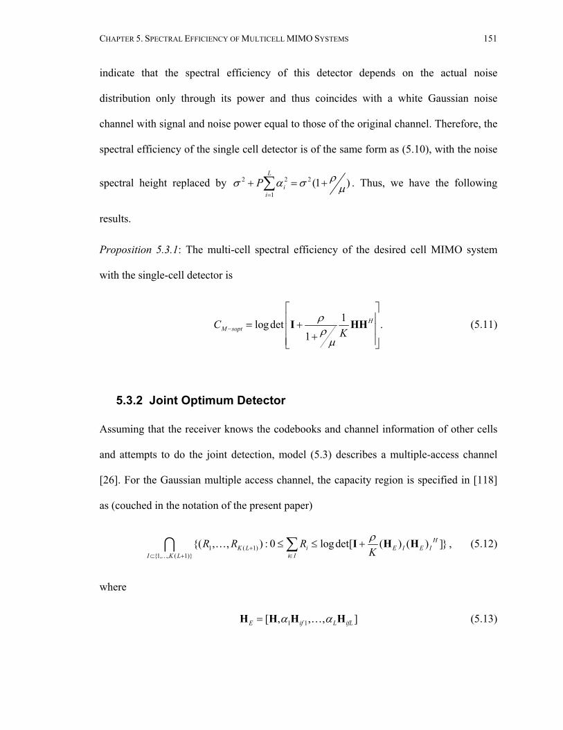
CHAPTER 5. SPECTRAL EFFICIENCY OF MULTICELL MIMO SYSTEMS 151
indicate that the spectral efficiency of this detector depends on the actual noise
distribution only through its power and thus coincides with a white Gaussian noise
channel with signal and noise power equal to those of the original channel. Therefore, the
spectral efficiency of the single cell detector is of the same form as (5.10), with the noise
spectral height replaced by 2 2 2
1(1 )
L
ii
P ρσ α σ µ=
+ = +∑ . Thus, we have the following
results.
Proposition 5.3.1: The multi-cell spectral efficiency of the desired cell MIMO system
with the single-cell detector is
1logdet .1
HM soptC
Kρρµ
−
= + +
I HH (5.11)
5.3.2 Joint Optimum Detector Assuming that the receiver knows the codebooks and channel information of other cells
and attempts to do the joint detection, model (5.3) describes a multiple-access channel
[26]. For the Gaussian multiple access channel, the capacity region is specified in [118]
as (couched in the notation of the present paper)
1 ( 1)1, , ( 1)
( , , ) : 0 logdet[ ( ) ( ) ]HK L i E I E I
i II K L
R R RKρ
+∈⊂ +
≤ ≤ +∑ I H H…
…∩ , (5.12)
where
1 1[ , , , ]E if L ifLα α=H H H H… (5.13)

CHAPTER 5. SPECTRAL EFFICIENCY OF MULTICELL MIMO SYSTEMS 152
and ( )E IH means the | |N I× submatrix of EH obtained by striking out the columns
whose indices do not belong to I, with | |I the cardinality of I. Here 1 ~ KR R denotes the
data rates of the MIMO system in the desired cell, 1 2~K KR R+ refers to that of the first
interfering cell with attenuation factor 1α , and so on. The following proposition is a
specific application of (5.12).
Proposition 5.3.2: The partial sum spectral efficiency of the multi-cell MIMO systems
with the joint optimum detector is
( ) log det[ ( ) ( ) ]J HM opt E J E JSR
Kρ
− = +I H H , (5.14)
where 0,1, , J L⊂ … denotes the set of cells of interest (cell 0 is the desired cell), and
( )E JH means the | |N J K× submatrix of EH obtained by striking out the channel
matrices of the interfering cells whose indices do not belong to J.
Corollary 5.3.1: The multi-cell spectral efficiency of the desired cell MIMO system with
the joint optimum detector is the same as that of the single-cell MIMO systems,
0M opt M opt S optC SR C− − −= = . (5.15)
Comments: Note that by employing a joint maximum likelihood detector at the receiver
of the desired cell, even though the data from the interfering cells may not be detected
correctly (the data rate of interfering cells exceeds the link capacity viewed at the receiver
of the desired cell), the data of the desired cell will be detected with high fidelity, as long
as the data rate of the desired cell is below its single-cell capacity.

CHAPTER 5. SPECTRAL EFFICIENCY OF MULTICELL MIMO SYSTEMS 153
5.3.3 Group Linear MMSE Detector As we mentioned in Chapter 4, joint maximum likelihood detection for multi-cell MIMO
is impractical for most current applications due to its complexity. With no intention to
detect the data from the interfering cells, group linear MMSE MUD is one of the most
favorable techniques to suppress the intercell interference. The detection process is to
first apply the weight matrix
1
2H Hi ifi ifi
i
Kαρ
−
= + +
∑W HH H H I H (5.16)
to the received signal (5.3) to combat the intercell interference, and then to optimally
detect the data of the desired cell .
When there is no attempt to detect the data from the interfering cells, model (5.3)
should be understood as a non-Gaussian interference channel in general. Even though the
non-Gaussian channel capacity is higher than that of the Gaussian channel with the same
input power constraint, it can hardly be approached due to the following reasons. First,
the noise characteristics are either not known exactly (e.g., in the interference channel) or
are too expensive to exploit. Second, capacity-approaching signaling for non-Gaussian
channels is far less well understood than that for the Gaussian channel. Therefore, the
Gaussian-based optimal metric is widely used in receiver design. It is shown in [65] and
[64] that, in the case of an ergodic additive non-Gaussian channel, when Gaussian
codebooks are used, a receiver that exploits a Gaussian-based optimal metric can not
surpass the Gaussian capacity, defined as follows.
Definition 5.3.1: The Gaussian capacity of an additive non-Gaussian channel is the
capacity of an additive Gaussian channel with the same noise covariance matrix.
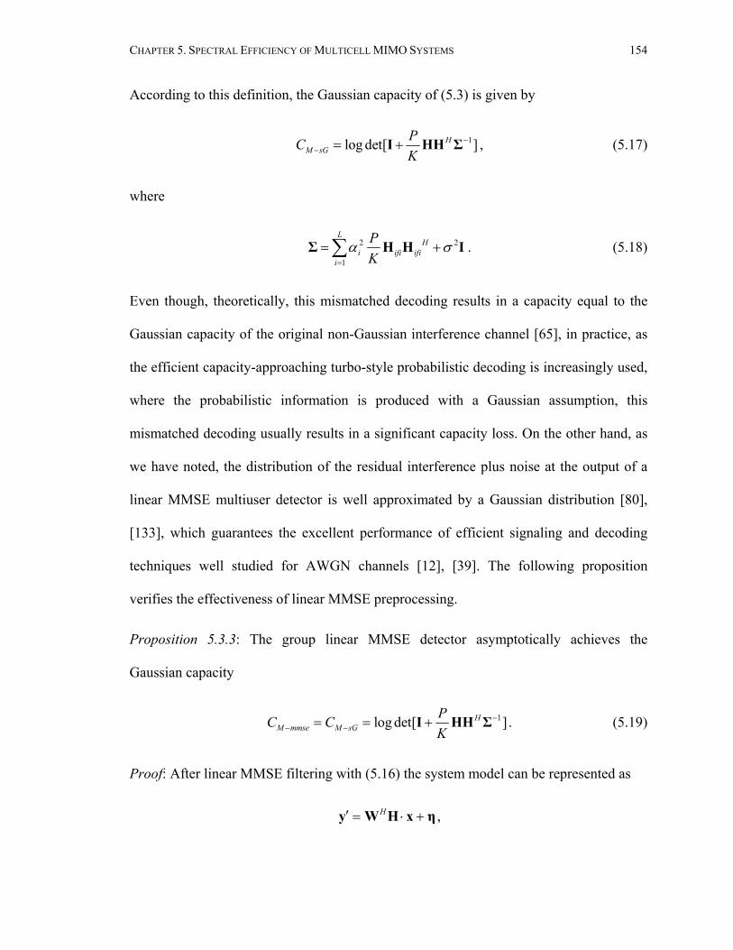
CHAPTER 5. SPECTRAL EFFICIENCY OF MULTICELL MIMO SYSTEMS 154
According to this definition, the Gaussian capacity of (5.3) is given by
1log det[ ]HM sG
PCK
−− = +I HH Σ , (5.17)
where
2 2
1
LH
i ifi ifii
PK
α σ=
= +∑Σ H H I . (5.18)
Even though, theoretically, this mismatched decoding results in a capacity equal to the
Gaussian capacity of the original non-Gaussian interference channel [65], in practice, as
the efficient capacity-approaching turbo-style probabilistic decoding is increasingly used,
where the probabilistic information is produced with a Gaussian assumption, this
mismatched decoding usually results in a significant capacity loss. On the other hand, as
we have noted, the distribution of the residual interference plus noise at the output of a
linear MMSE multiuser detector is well approximated by a Gaussian distribution [80],
[133], which guarantees the excellent performance of efficient signaling and decoding
techniques well studied for AWGN channels [12], [39]. The following proposition
verifies the effectiveness of linear MMSE preprocessing.
Proposition 5.3.3: The group linear MMSE detector asymptotically achieves the
Gaussian capacity
1log det[ ]HM mmse M sG
PC CK
−− −= = +I HH Σ . (5.19)
Proof: After linear MMSE filtering with (5.16) the system model can be represented as
H′ = ⋅ +y W H x η ,

CHAPTER 5. SPECTRAL EFFICIENCY OF MULTICELL MIMO SYSTEMS 155
where η is Gaussian distributed with covariance matrix of HW ΣW . This is verified in
[133] as N →∞ . The spectral efficiency of this model is given by
1log det[ ( ) ]H H HM MMSE
PCK
−− = +I W HH W W ΣW . (5.20)
With (5.16) and (5.18), it is easy to verify that
( )H H HPK
= −W ΣW I W H W H .
Assume K N≤ throughout, and define 1HPK
−=Q H Σ H , it is shown that the probability
that Q is non-singular goes to 1 as N →∞ [120]. Then
1
1 1 1 1
( )
( ( ) ( )) ,
H H H
H H
KP
P P PK K K
−
− − − −
= +
= −
W H H HH Σ H
H Σ Σ H∆ H Σ H
with 1( )H PK
−= + = +∆ I H Σ H I Q , by the matrix inverse formula. It then follows that
1 1( ) ( )H − −= − + = +W H Q Q I Q Q I Q Q , and 1 1( ) ( )H − −− = − + = +I W H I I Q Q I Q , both
of which are invertible asymptotically.
Therefore (note H H=W H H W )
1
1
1 1
log det[ ( ) ]
log det[( ) ]log det[( ( ) ) ]log det[ ] .
H HM mmse
H
M sG
C
C
−−
−
− −
−
= + −
= −
= − += + =
I W H I W H
I W HI I Q Q
I Q
(5.21)
QED.

CHAPTER 5. SPECTRAL EFFICIENCY OF MULTICELL MIMO SYSTEMS 156
By Proposition 5.3.3, we have the following consequence.
Corollary 5.3.2: The multi-cell spectral efficiency of the desired MIMO system with the
linear MMSE detector is
0,1, , 1, , L LM mmse M opt M optC SR SR− − −= −… … . (5.22)
Proof: By (5.18),
2 2
1
2( ) .
LH
i ifi ifii
H HE E
PK
PK
α σ
σ
=
= +
= − +
∑Σ H H I
H H HH I
So
2
1( )H HE EK
ρσ
− = −H H HH Σ I
and
2
1H HE EK K
ρ ρσ
= + −H H HH Σ I
Therefore,
1
( )
HE E
H
H HE E
P KK
K
ρ
ρ−
++ =
+ −
I H HI HH Σ
I H H HH. (5.23)
Compare (5.14) and (5.19), (5.22) follows.
QED.

CHAPTER 5. SPECTRAL EFFICIENCY OF MULTICELL MIMO SYSTEMS 157
In general, if we partition the cells in two groups, applying the linear MMSE
decoding to one of them while treating the other as interfering cells, the sum spectral
efficiency is exactly analogous to (5.22). Thus, we have the following.
Corollary 5.3.3: The partial sum spectral efficiency of multi-cell MIMO systems with the
generalized group linear MMSE detector is
0,1, , ( ) ( )LJ JM mmse M opt M optSR SR SR− − −= −… , (5.24)
where 0,1, , J L⊂ … denotes the set of cells of interest (cell 0 is the desired cell), and
J is the complement of J in 0,1, , L… .
Comments: Note that 0M mmse M mmseSR C− −= , while 0,1, , 0,1, , L L
M mmse M optSR SR− −=… … . Within the set of
cells of interest J, while treating the interference from other cells as Gaussian background
noise (due to MMSE processing), we can similarly define a multiple access capacity
region as Proposition 5.3.2. Denote a set K J⊂ , then the partial sum spectral efficiency
of this set is given by
( , ) 1log det ( ) ( )J K HM mmse E K E K J
PSRK
−−
= + I H H Σ , (5.25)
where 2 2Hi ifi ifiJ
i J
PK
α σ∈
= +∑Σ H H I . Similarly (5.25) can be represented by
( , ) ( ) ( ) .J K K J JM mmse M opt M optSR SR SR∪− − −= − (5.26)

CHAPTER 5. SPECTRAL EFFICIENCY OF MULTICELL MIMO SYSTEMS 158
5.3.4 Group MMSE Successive Cancellation Detector As noted previously, since joint maximum likelihood detection for multi-cell MIMO is
highly complex, while linear MMSE MUD is limited in its interference cancellation
capability, especially when 1β ≥ [120], non-linear multiuser detection often provides a
favorable tradeoff between performance and complexity. Group MMSE successive
cancellation is one such technique, in which information bits are detected by group linear
MMSE detection cell by cell, with the interference from previously detected cells already
being subtracted. Although successive cancellation does not result in maximum-
likelihood decisions, it becomes asymptotically optimal as the error probability of
intermediate decisions vanishes with code block length [116]. With the assumption of
perfect cancellation, the following lemma shows the optimality of group MMSE
successive interference cancellation.
Lemma 5.3.1: Multi-cell MIMO systems with the group MMSE successive cancellation
detector applied to the set of cells of interest 0,1, , J L⊂ … achieves some vertices of
the capacity region given by (5.25) and (5.26).
Proof: Suppose 1 | | , , JJ i i= … . Without loss of generality, suppose also that the cells are
decoded in that order. Following Corollary 5.3.2, and assuming perfect cancellation of
the interference from the detected cells, we have
0,1, , \ 0,1, , 1 1( ) L iLiM sic M opt M optC SR SR− − −= − ……
0,1, , \ 0,1, , \ , 2 1 1 2( ) L i L i iiM sic M opt M optC SR SR− − −= −… …

CHAPTER 5. SPECTRAL EFFICIENCY OF MULTICELL MIMO SYSTEMS 159
0,1, , \ , , 0,1, , \| | 1 | | 1( ) L i i L JJ JiM sic M opt M optC SR SR−
− − −= −… … … . (5.27)
Equivalently, the above | |J equalities can be reformulated as
| | | | | |( , ) ( ) ( )i JJ J JJ i i JM sic M sic M opt M optSR C SR SR∪
− − − −= = −
, | | 1 | | | | 1 | | | | 1 | |( , , ) ( ) ( ) ( )i i JJ J J J J JJ i i i i JM sic M sic M sic M opt M optSR C C SR SR∪− − −
− − − − −= + = −
0,1, , | | 1 | |1 ( ) ( )( )( ) ( )LJ Ji iiJ JM sic M sic M sic M sic M opt M optSR C C C SR SR−
− − − − − −= + + + = −… . (5.28)
On comparing (5.28) with (5.26), we see that one of the vertices of the Gaussian multiple
access capacity region is achieved.
As the MMSE successive interference cancellation detector has | | !J different orders
of detection, | | !J vertices of the capacity region in the | |JR domain can be achieved. As
the capacity region of the multiple-access channel is convex, by timesharing, the MMSE
successive interference cancellation detector can thus achieve the capacity region
spanned by these vertices.
QED.
Corollary 5.3.4:
0,1, , ( ) ( ) ( ) ( )LJ i J JM sic M sic M opt M opt M mmse
i JSR C SR SR SR− − − − −
∈
= = − =∑ … . (5.29)
0 0M sic M mmse M mmseSR SR C− − −= = . (5.30)
0,1, , 0,1, , 0,1, , L L LM sic M mmse M optSR SR SR− − −= =… … … . (5.31)

CHAPTER 5. SPECTRAL EFFICIENCY OF MULTICELL MIMO SYSTEMS 160
To achieve some vertex of the capacity region of the Gaussian multiple access
channel that corresponds to the maximum rate for the desired cell (single cell capacity),
Lemma 5.3.1 suggests a detection order that puts the detection of the desired cell last. For
example, suppose the cells are detected in the order of , 1, ,0L L − … , the achieved
capacity vertex is given by
( ) (1) (0)( , , , )LM sic M sic M sicR R R− − −… , (5.32)
with
0,1, , 0,1, , 1( ) , 0,1, ,l llM sic M opt M optR SR SR l L−
− − −= − =… … … . (5.33)
Clearly,
0(0)M sic M opt S optR SR C− − −= = . (5.34)
Note that in practice, the success of interference cancellation relies highly on the
correct detection of interference. In adverse environments where we cannot get good
estimates of interference, successive interference cancellation schemes will worsen the
performance instead of improving it. Therefore, to achieve the optimum capacity of
(5.34), the MMSE successive interference cancellation detector implicitly requires that
the data rates of other interfering cells satisfy (5.33). This is impractical, as it requires not
only joint signaling but also puts the desired cell in a superior position. What is of
practical interest is that all cells are autonomous with identical data rates. This identical
rate tuple can in general be achieved by timesharing. With this restriction, the following
proposition shows the limitation of the MMSE successive interference cancellation
detector.

CHAPTER 5. SPECTRAL EFFICIENCY OF MULTICELL MIMO SYSTEMS 161
Proposition 5.3.4: Assuming that the same data rate is employed in each cell, and that
10 1Lα α≤ ≤ ≤ ≤ , the multi-cell spectral efficiency of the desired cell MIMO system
with the group MMSE successive cancellation detector applied to the cells 0,1, , J l= …
is
1, , 1, ,
( )
1, , 1min , 0,1, ,
l k L l LM opt M optl
M sic k l
SR SRC l L
k
− + +
− −− = +
−= =
… …
…… . (5.35)
Proof: As the same data rate is employed in each cell, we have
( , ) ( )J K lM sic M sicSR K C− −= . (5.36)
We know from Lemma 5.3.1 that the achievable rate-tuples are constrained by (5.26).
Due to the condition 10 1Lα α≤ ≤ ≤ ≤ , we can rule out most of the constraints. For
single rate, we have
( ) 1, , ( ) 1, ,
, , 1, ,
min
.
ji l Ll l LM sic M opt M optj J
l L l LM opt M opt
C SR SR
SR SR
∪ + +− − −⊂
+− −
≤ −
= −
… …
… … (5.37)
Similarly, for sum rates of two cells, we have
( ) , 1, , ( ) 1, ,
,
1, , 1, ,
2 min
.
j ki i l Ll l LM sic M opt M optj k J
l L l LM opt M opt
C SR SR
SR SR
∪ + +− − −⊂
− +− −
≤ −
= −
… …
… … (5.38)
So,
1, , 1, ,
( ) ( ).2
l L l LM opt M optl
M sic
SR SRC
− +
− −−
−≤
… …
(5.39)
By a similar argument, (5.35) follows readily.
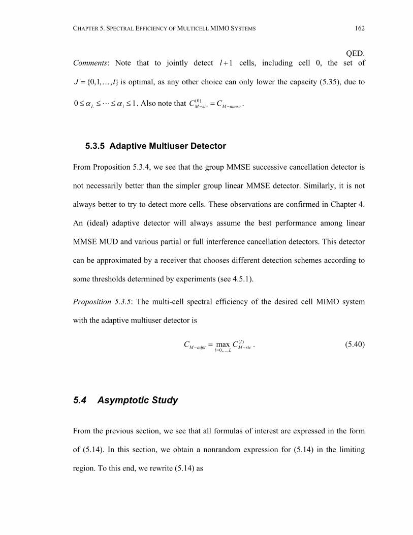
CHAPTER 5. SPECTRAL EFFICIENCY OF MULTICELL MIMO SYSTEMS 162
QED. Comments: Note that to jointly detect 1l + cells, including cell 0, the set of
0,1, , J l= … is optimal, as any other choice can only lower the capacity (5.35), due to
10 1Lα α≤ ≤ ≤ ≤ . Also note that (0)M sic M mmseC C− −= .
5.3.5 Adaptive Multiuser Detector From Proposition 5.3.4, we see that the group MMSE successive cancellation detector is
not necessarily better than the simpler group linear MMSE detector. Similarly, it is not
always better to try to detect more cells. These observations are confirmed in Chapter 4.
An (ideal) adaptive detector will always assume the best performance among linear
MMSE MUD and various partial or full interference cancellation detectors. This detector
can be approximated by a receiver that chooses different detection schemes according to
some thresholds determined by experiments (see 4.5.1).
Proposition 5.3.5: The multi-cell spectral efficiency of the desired cell MIMO system
with the adaptive multiuser detector is
( )
0, ,max l
M adpt M sicl LC C− −=
=…
. (5.40)
5.4 Asymptotic Study From the previous section, we see that all formulas of interest are expressed in the form
of (5.14). In this section, we obtain a nonrandom expression for (5.14) in the limiting
region. To this end, we rewrite (5.14) as

CHAPTER 5. SPECTRAL EFFICIENCY OF MULTICELL MIMO SYSTEMS 163
( )
1
lim lim log det ( ) ( )
1lim log det ( ) ( )
1lim log 1
log 1 ,
J HM opt E J E JN N
HE J E JN
N
iN i
SRK
N
NN
NE
ρ
ρβ
ρ λβ
ρ λβ
−→∞ →∞
→∞
→∞ =
= +
= +
= +
= +
∑
I H H
I H H
(5.41)
where iλ are the eigenvalues of
1
1 | | 1 | |
| |
2
2
1 1( ) ( ) [ , , ] [ , , ]J J
J
i
H HE J E J i i i i
i
N N
α
α
=
H H H H H H… … . (5.42)
To calculate (5.41), notice that
( ) log(1 )Eγ γλ= +C (5.43)
is an increasing function of γ with (0) 0=C , so we can express (5.43) as
0
0
( ) ( )
.1
d x dxdx
E dxx
γ
γ
γ
λλ
=
= +
∫
∫
C C (5.44)
Further notice that (5.42) conforms with the conditions of Theorem 5.2.1, so the
empirical eigenvalue distribution of 1 ( ) ( ) HE J E JN
H H converges in distribution to a
nonrandom distribution function Q, whose Stieltjes transform ( )Qm z is a unique solution
to

CHAPTER 5. SPECTRAL EFFICIENCY OF MULTICELL MIMO SYSTEMS 164
2| |
21 .
1( )| | ( )
1 ( )
1
1 ( )j
j
Q
Q
Ji
j i Q
m zz J dH
m z
zm z
τβ ττ
αβ
α=
=− +
+
=
− ++
∫
∑
(5.45)
By (5.4), we have
1( )Qm z Ezλ
= − . (5.46)
So,
2
1( )
1
Qx mxE
x xλλ
− − = + . (5.47)
Therefore,
( )/
20
1
lim JQ
M optN
x mxSR N dx
xρ β
−→∞
− − = ∫ , (5.48)
where ( )Qm x is an implicit solution of (5.45).
The optimum spectral efficiency of single-cell MIMO systems (5.10) can be
calculated in the same way as above. However, due to the expression of (5.9), a closed-
form expression can be derived as follows. In the limiting region, we can express (5.10)
as
1
1lim lim log(1 )
log(1 ).
N
S opt iN N i
C NN
NE
ρλ
ρλ
−→∞ →∞=
= +
= +
∑ (5.49)

CHAPTER 5. SPECTRAL EFFICIENCY OF MULTICELL MIMO SYSTEMS 165
where iλ are the eigenvalues of 1 H
KHH , whose limiting probability density function
is given by (5.9). Using the same differentiation-integration strategy, we have
0
0
lim1
1 11 .1
S optNC N E dx
x
N E dxx x
ρ
ρ
λλ
λ
−→∞
= + = − +
∫
∫ (5.50)
Fortunately, 11
Exλ
+
can be calculated explicitly:
1
1( )
1( )
( )
( )
1 1 ( )1 1
1 1[ ( )][ ( ) ]1(1 ) 11 2 ( )
[ ( )][ ( ) ]1(1 )21
1(1 ) 1 ( , )4
1 ( , ),4
b
a
b
a
E f dx x
a bd
x
a bdx
xx
xx
β
β
β
β
β
λ λλ λ
λ λβ ββ λ
λ π λβ
ω β β ωβ β ω
πβωωβ
β β ββ
β ββ
= + +
− −= − +
+
− −= − +
+
= − + −
= −
∫
∫
∫
F
F
(5.51)
where the second-to-last definite integral is derived in [49], [120], and the function
( , )x zF is given in (5.7). Finally,
20
/
20
lim ( , )4
1 ( , )4
( , ),
S optNxC N dx
x
N y dyy
N
ρ
ρ β
β ββ
β
ρ ββ
−→∞=
=
=
∫
∫
F
F
G
(5.52)

CHAPTER 5. SPECTRAL EFFICIENCY OF MULTICELL MIMO SYSTEMS 166
where
1 14 4
log( , ) log(1 ( , )) log(1 ( , )) ( , )4
ex z z x x z xz x z x zx
= + − + + − −G F F F . (5.53)
Similarly, we have
lim ( , ).(1 / )M soptNC N ρ βρ µ β−→∞
= +G (5.54)
5.5 Some Analytical and Numerical Results In this section, some analytical and numerical results are given as applications of the
above derived formulas, from which we can get some insights into the behavior of multi-
cell MIMO systems. Unless otherwise specified, we assume such a multicell model
having four interferers in two groups of two, in which one group is 6 dB stronger than the
other while the users within each group have the same power. This roughly reflects the
essential reality as interference from the two farthest adjacent cells can typically be
ignored, and simulation results in Chapter 4 verify that the power of the two strongest
users usually dominates. Therefore, we assume the following parameters for (5.3): 4L =
and
2 11
1
22
1
2 23
2
24
2
1 ,1 1
1 1 ,1 1
1 1 ,1 1
1 1 1 ,1 1
γ βαµ γ β
γαµ γ β
βαµ γ β
αµ γ β
=+ +
=+ +
=+ +
=+ +
(5.55)

CHAPTER 5. SPECTRAL EFFICIENCY OF MULTICELL MIMO SYSTEMS 167
with 1 24, 1,and 1γ β β= = = . Recall that µ is the SIR. Further, as spectral efficiencies
of MIMO systems grow linearly with the number of receive antennas N, in our study we
are mainly interested in normalized spectral efficiencies per receive antenna. The reader
should keep this in mind when interpreting the overall MIMO capacity from the
following figures.
5.5.1 Approximate Formula The exact formula of (5.48) requires numerical fixed-point solutions of (5.45) and the
definite integral of (5.48), which is fairly complex. So, an approximating formula of
(5.14) is explored here. The key idea is to approximate ( ) ( ) HE J E JH H as
2
( ) ( ) ( )| |
iH Hi J
E J E J J
α⊂ ′ ′≈∑
H H H H , (5.56)
where ′H denotes an | |N K J× random matrix with i.i.d. normalized complex Gaussian
entries. In this way, a closed-form formula similar to (5.52) can be obtained. Note that
even though we assume 1β ≤ all through the chapter, we should discern here whether
1| |Jβ ≤ , which determines whether the empirical eigenvalue distribution of
2
1 ( ) ( ) HE J E J
ii J
K α⊂∑
H H has a mass point at 0 (see (5.9)). Following the same lines as
(5.52), we get the following approximate formula for (5.14), which coincides for all
values of β :

CHAPTER 5. SPECTRAL EFFICIENCY OF MULTICELL MIMO SYSTEMS 168
( ) 2
2
1lim | | , | |
, | | .| |
JM opt iN i J
ii J
SR N J J
N JJ
β ρ α β
ρ αβ
β
−→∞ ⊂
⊂
≈
=
∑
∑
G
G (5.57)
We will see in the following that (5.57) gives a good enough approximation for a wide
range of parameter settings. It tends to overestimate when β is small or there is great
discrepancy within the set of iα of interest. Even in this case, (5.57) roughly exhibits
the same behavior as (5.48), and thus is still useful for theoretical analysis.
5.5.2 Interference-Limited Behavior Clearly, the single-cell detector is interference limited, which can be verified by (5.54):
lim ( , ) ( , )(1 / )ρ
ρ µβ βρ µ β β→∞=+G G . (5.58)
Even though for 1β = , the group linear MMSE detector is also interference limited (see
Chapter 4), we noted that it is due to the lack of sufficient degrees of freedom at the
receiver to suppress the co-channel interference. We believe that if β is sufficiently
small, the group linear MMSE detector is not interference limited. This is verified in Figs
5.1 (a)-(c). Here the SIR is set to be 0 dB, indicating a strong interference environment. It
is observed in these figures that the spectral efficiency of the single cell upper bound (see
(5.52)) and that of the single-cell detector (see (5.54)) decrease as the system load β
decreases. The single-cell detector is interference-limited, with the limiting value being
given by (5.58). The spectral efficiency of the group linear MMSE detector, both the
exact (see (5.24) and (5.48)) and the approximate (see (5.24) and (5.57)), however,

CHAPTER 5. SPECTRAL EFFICIENCY OF MULTICELL MIMO SYSTEMS 169
increases as β decreases, when the SNR is sufficiently large. Furthermore, when the
system load decreases to 1/5, the group linear MMSE detector is not interference limited.
Comparing Figs 5.1 (a), (c) with (d), where a more favorable SIR = 5 dB is experienced,
we can see that all the multicell spectral efficiencies increase as SIR increases. However,
due to the interference-limited nature, the spectral efficiency of the group linear MMSE
detector with system load 1 is outperformed by the same detector with system load of 1/5
at a much worse SIR, when the SNR is sufficiently large. This observation is helpful for
multicell MIMO system design. Finally, we observe that the approximate formula well
matches the exact one, thus providing a valuable tool for analysis.
Let us turn to the normalized approximate formula, given as
(1 1/ ) (1/ )lim / ( , , ) , ( 1) ,( 1)M mmseN
C N L LL L
ρ µ ρ µρ µ β β ββ β−→∞
+≈ + − +
R G G , (5.59)
to study the interference-limited behavior of the group linear MMSE detector. In the
Appendix I, we show that
1lim ( , , ) log(1 ) (1 ( 1)) log 1( 1) 1when >
L1( 1) log 1
LL
LL
ρρ µ β µ β
ββ
ββ
→∞
= + + − + − +
+ − −
R
, (5.60)
and
1lim ( , , ) whenL+1ρ
ρ µ β β→∞
= ∞ ≤R . (5.61)

CHAPTER 5. SPECTRAL EFFICIENCY OF MULTICELL MIMO SYSTEMS 170
The analytical results of (5.60) and (5.61) agree with the numerical results of Fig. 5.1
very well. The “magic” number 1/5 is not found by luck but rather is determined by the
system behavior.
0 5 10 15 20 25 300
0.5
1
1.5
2
2.5
3SIR = 0dB, System Load = 1
SNR (dB)
Nor
mal
ized
Spe
ctra
l Effi
cien
cy (b
its/s
/Hz/
ante
nna)
Single cell upper bound Group linear MMSE-approx.Group linear MMSE Single-cell decoder
(a)

CHAPTER 5. SPECTRAL EFFICIENCY OF MULTICELL MIMO SYSTEMS 171
0 5 10 15 20 25 300
0.5
1
1.5
2
2.5
3SIR = 0 dB, System Load = 1/2
SNR (dB)
Nor
mal
ized
Spe
ctra
l Effi
cien
cy (b
its/s
/Hz/
ante
nna) Single cell upper bound
Group linear MMSE-approx.Group linear MMSE Single-cell decoder
(b)
0 5 10 15 20 25 30 350
0.5
1
1.5
2
2.5
3SIR = 0 dB, System Load = 1/5
SNR (dB)
Nor
mai
lzed
Spe
ctra
l Effi
cien
cy (b
its/s
/Hz/
ante
nna)
Single cell upper bound Group linear MMSE-approx.Group linear MMSE Single-cell decoder
(c)

CHAPTER 5. SPECTRAL EFFICIENCY OF MULTICELL MIMO SYSTEMS 172
0 5 10 15 20 25 300
0.5
1
1.5
2
2.5
3SIR = 5 dB, System load = 1
SNR (dB)
Nor
mal
ized
Spe
ctra
l Effi
cien
cy (b
its/s
/Hz/
ante
nna)
Single cell upper bound Group linear MMSE-approx.Group linear MMSE Single-cell decoder
(d)
Fig. 5.1 Study of interference-limited behavior of various multicell MIMO spectral efficiencies
5.5.3 Adaptive Detection We continue to study the behavior of the group MMSE successive cancellation detector
(see (5.35)) and the adaptive multiuser detector (see (5.40)). The asymptotic spectral
efficiencies given in this subsection are calculated with the exact formula (5.48). In the
following figures, we use “Group MMSE SC-l” to denote the multi-cell spectral
efficiency of the desired MIMO system with the group MMSE successive cancellation
detector applied to the cells 0,1, , J l= … . The group linear MMSE detector corresponds
to “Group MMSE SC-1”, and the adaptive detector achieves the best among these
detectors.

CHAPTER 5. SPECTRAL EFFICIENCY OF MULTICELL MIMO SYSTEMS 173
From Figs 5.2 (a) and (b) we see that, for a fairly high SIR, the simpler group linear
MMSE detector is the best; but in a strong interference environment, group MMSE
successive cancellation proves to be useful. This verifies the well-known fact that,
detection of the interfering users is only optimal in the strong-interference case; for weak
interference, it is better to simply treat them as ambient noise. It is also observed that, in
the sufficiently high SNR scenario, the group MMSE successive cancellation detector
applied to all the cells eventually stands out; but for other cases, trying to detect more
cells actually lowers the possible achieved capacity. This is more evident in Fig. 5.2 (c),
where a one-dominant-interferer scenario with 1 23.5, 6, 1γ β β= = = (the power of the
strongest interferer is 3 dB higher than the power sum of the rest interferers) is assumed.
We find that for low to medium SNR, detection of only the strongest interferer is the best,
while full MMSE successive cancellation is the best in the high SNR regime.
In Fig. 5.3 (a), we show the spectral efficiency of the ideal adaptive detector for
different SNR and SIR scenarios. We assume the model of (5.55) with
1 24, 1, 1γ β β= = = , and with system load 1. We also show the single cell upper bound
and that of the single-cell detector for reference. We see that multiuser detection across

CHAPTER 5. SPECTRAL EFFICIENCY OF MULTICELL MIMO SYSTEMS 174
0 5 10 15 20 25 300
0.5
1
1.5
2
2.5
SNR (dB)
Nor
mal
ized
Spe
ctra
l Effi
cien
cy (b
its/s
/Hz/
ante
nna)
SIR = 5 dB, System Load = 1
Group linear MMSEGroup MMSE SC-2 Group MMSE SC-3 Group MMSE SC-4 Group MMSE SC-5 Adaptive decoder
(a)
0 5 10 15 20 25 300
0.5
1
1.5
2
2.5
SNR (dB)
Nor
mal
ized
Spe
tral E
ffici
ency
(bits
/s/H
z/an
tenn
a)
SIR = 0 dB, System Load = 1
Group linear MMSEGroup MMSE SC-2 Group MMSE SC-3 Group MMSE SC-4 Group MMSE SC-5 Adaptive decoder
(b)

CHAPTER 5. SPECTRAL EFFICIENCY OF MULTICELL MIMO SYSTEMS 175
0 5 10 15 20 25 300
0.5
1
1.5
2
2.5
SNR (dB)
Nor
mal
ized
Spe
ctra
l Effi
cien
cy (b
its/s
/Hz/
ante
nna)
SIR = 0 dB, System Load =1, One dominant Interferer
Group linear MMSEGroup MMSE SC-2 Group MMSE SC-3 Group MMSE SC-4 Group MMSE SC-5 Adaptive decoder
(c)
Fig. 5.2 Spectral efficiency comparison of group linear MMSE detector, group MMSE successive cancellation detector, and adaptive detector
0 5 10 15 20 25 300
1
2
3
4
5
6
7
8
9
SNR (dB)
Nor
mal
ized
Spe
ctra
l Effi
cien
cy (b
its/s
/Hz/
ante
nna)
System Load = 1
Single cell upper bound Adaptive decoder-20dB Single-cell decoder-20dBAdaptive decoder-10dB Single-cell decoder-10dBAdaptive decoder-5dB Single-cell decoder-5dB Adaptive decoder-0dB Single-cell decoder-0dB
(a)

CHAPTER 5. SPECTRAL EFFICIENCY OF MULTICELL MIMO SYSTEMS 176
0 5 10 15 20 25 300
0.5
1
1.5
2
2.5
SNR (dB)
Nor
mal
ized
Spe
ctra
l Effi
cien
cy (b
its/s
/Hz/
ante
nna)
System Load = 1/5
Single cell upper bound Adaptive decoder-20dB Single-cell decoder-20dBAdaptive decoder-10dB Single-cell decoder-10dBAdaptive decoder-5dB Single-cell decoder-5dB Adaptive decoder-0dB Single-cell decoder-0dB
(b)
Fig. 5.3 Multicell MIMO capacity for different SNRs and SIRs the cell is most useful in the strong interference environment. Its advantage over the
single-cell detector diminishes as SIR increases. However, note that in practice, while the
group linear MMSE capacity (which is also the adaptive detector capacity in high SIR,
see Fig. 5.2 (a)) can be closely approached, there is no effective way to approach the
single-cell detector capacity due to the non-Gaussian nature of the channel. Also note that
a small difference in the spectral efficiency per receive antenna may become substantial
in large systems. In the strong interference environment, even though multiuser detection
across the cell brings substantial gain over single-cell detection, there is a substantial gap
between the achievable capacity and the single cell upper bound. This is not the case for
sufficiently low system load, as is shown in Fig. 5.3 (b). However, as the system load is
reduced, the achievable capacity is also reduced. In the strong interference environment,
it is possible to improve the system performance by reducing the system load and

CHAPTER 5. SPECTRAL EFFICIENCY OF MULTICELL MIMO SYSTEMS 177
increasing the signal power, though this may be costly. In the low interference
environment, however, it is better to have a high system load and a group linear MMSE
receiver.
5.6 Summary In this chapter, the spectral efficiency of multicell MIMO systems with several MUD
detectors has been studied, among which are a single-cell detector, the joint optimum
detector, a group linear MMSE detector, a group MMSE successive cancellation detector,
and an adaptive multiuser detector. The large-system asymptotic (non-random)
expressions for these spectral efficiencies have also been explored.
As applications of these theoretical bounds, we have verified the following
observations from Chapter 4 about multicell MIMO systems. Group linear MMSE
detection and group MMSE successive cancellation are two effective techniques to
combat the co-channel interference, each of which may outperform the other for different
settings. Based on this observation, an adaptive detector was developed to attempt to
achieve the better of the two. For full system load, multiuser detection across the cell is
most useful in strong interference environments, offering substantial gain over traditional
single-cell detection. However, there is still a remarkable gap between the achievable
capacity and the single cell upper bound in this case.
Further, conditions for non-interference-limited behavior of the group linear MMSE
detector have been found. Based on this result, it is suggested that with sufficiently low

CHAPTER 5. SPECTRAL EFFICIENCY OF MULTICELL MIMO SYSTEMS 178
system load 11L
β ≤+
, where L is the number of effective interfering cells, better
performance than that of the fully loaded system may be attained in the strong
interference environment with sufficiently large signal power. If the interference is weak,
then a high-load system with fairly simple group linear MMSE detection has the
advantage.
Appendix I
First let us examine the limiting behavior of the three parts of ( , )x zG in (5.53):
( , )lim min( ,1)4x
x z zx→∞
=F , (5.62)
14
1 1lim1 ( , ) lim ( , ) min( ,1)1 14x x
x x z x z zzx z
→∞ →∞+ − = =
− −F
F, (5.63)
14
1 1lim1 ( , ) lim ( , ) 1 min( ,1)1 4x x
xz x z x z zx
→∞ →∞+ − = =
−−F
F. (5.64)
We see that when 1z ≤ , (5.63) goes to infinity, and when 1z ≥ , (5.64) goes to infinity.
Expanding (5.59), we have
1 2 3( , , ) ( , , ) ( , , ) ( , , )ρ µ β ρ µ β ρ µ β ρ µ β= + +R R R R , (5.65)
where
1 1 2 21
1 2
( , ) ( , )( , , ) log4 4x z x zex x
ρ µ β
= − −
F FR , (5.66)
1 12 1 1 1 1 2 2 2 24 4( , , ) log(1 ( , )) log(1 ( , ))z x x z z x x zρ µ β = + − − + −R F F , (5.67)

CHAPTER 5. SPECTRAL EFFICIENCY OF MULTICELL MIMO SYSTEMS 179
1 13 1 1 1 1 2 2 2 24 4( , , ) log(1 ( , )) log(1 ( , ))x z x z x z x zρ µ β = + − − + −R F F , (5.68)
with 1(1 1/ )
( 1)x
Lρ µβ+
=+
, 1 ( 1)z Lβ= + , 2(1/ )x
Lρ µβ
= , and 2z Lβ= .
If 1L
β > , then 1 1z > , and 2 1z > . By (5.62) we have
1lim ( , , ) 0ρ
ρ µ β→∞
=R . (5.69)
By (5.63) we have
21 1lim ( , , ) ( 1) log log1 11 1( 1)
xL L
L Lρ µ β β β
β β→∞
= + −− −+
R . (5.70)
3lim ( , , )ρ
ρ µ β→∞
R is in the form of log ∞∞
. By L'Hopital's rule, we have
11 1 1 141
1 1 1 141
12 2 2 242 2 2 24
11
22
(1 ( , ))1 ( , )lim lim1 ( , ) (1 ( , ))
(1 1/ ) ( 1),1/ ( 1)
x z x zx z x zx z x z x z x z
zz
zz
ρ ρ
ρ
ρµ
µ
→∞ →∞
∂ + −+ − ∂=
∂+ − + −∂
+−
=−
FFF F
(5.71)
where we use the fact that
1
11 1 1 1 14
1
lim (1 ( , )) 1x
x z x z zx→∞
∂+ − = −
∂F (5.72)
when 1 1z > . Equation (5.60) follows after simple calculation.
If 11L
β ≤+
, then 1 1z ≤ , and 2 1z < . We have

CHAPTER 5. SPECTRAL EFFICIENCY OF MULTICELL MIMO SYSTEMS 180
1
1 1 1412 1 2 1 1 1 24 1
2 2 24
1 ( , )lim ( , , ) ( ) log(1 ( , )) log( )1 ( , )
x x zz z x x z zx x zρ
ρ µ β→∞
+ −= − + − +
+ −F
R FF
. (5.73)
Similarly,
11 1 141
1 1 141
12 2 242 2 24
11
22
(1 ( , ))1 ( , )lim lim1 ( , ) (1 ( , ))
(1 1/ ) (1 ),1/ (1 )
x x zx x zx x z x x z
zz
zz
ρ ρ
ρ
ρµ
µ
→∞ →∞
∂ + −+ − ∂=
∂+ − + −∂
+−
=−
FFF F
(5.74)
where we use the fact that
1
11 1 1 14
1
lim (1 ( , )) 1x
x x z zx→∞
∂+ − = −
∂F (5.75)
when 1 1z ≤ . As 1 2z z> , by (5.63) we have
2lim ( , , )ρ
ρ µ β→∞
= ∞R , (5.76)
and (5.61) follows.

181
Chapter 6
Turbo Multiuser Detection for DSL Communications
6.1 Introduction In this chapter, we apply some of the receiver techniques discussed in the preceding
chapters to wireline communications. In particular, the turbo multiuser detection
techniques are applied to digital subscriber line (DSL) wireline communications to
effectively combat crosstalk, with the influence of impulse noise taken into consideration.
DSL technology provides transport of high-bit-rate digital information over telephone
subscriber lines. Various DSL techniques (Basic Rate integrated service digital network
(ISDN), high-rate DSL (HDSL), asymmetric DSL (ADSL), and very-high-rate DSL
(VDSL)) involving sophisticated digital transmission schemes and extensive signal
processing have recently become practical due to advances in microelectronics. The latest
in DSL technology is VDSL, which provides tens of megabits per second to those
customers who desire broadband entertainment or data services. At such high rates,
signals on twisted pairs can be reliably transmitted at most to a few thousand feet. Thus,
VDSL will primarily be used for loops fed from an optical network unit (ONU) or a
central office (CO) to a customer premises, i.e., it addresses the so-called “last mile”
problem. The modulation scheme for VDSL can either be multicarrier-based or single

CHAPTER 6. TURBO MULTIUSER DETECTION FOR DSL COMMUNICATIONS 182
carrier-based, typically discrete multitone (DMT) and carrierless amplitude/phase
modulation (CAP)/quadrature amplitude modulation (QAM). The duplexing methods can
be either time-division duplex (TDD) or frequency-division duplex (FDD) [23], [102].
Intersymbol interference (ISI) is one of the major obstacles to high-data-rate,
bandwidth-efficient communications. Multicarrier modulation (MCM), following
Shannon’s optimum transmission suggestion, achieves the highest performance in
channels with ISI. DMT is a particular form of MCM that has been found to be well
suited for DSL application and is adopted in ANSI T1.413 ADSL standards. With this
approach, a channel is divided into many independent ISI-free subchannels in the
frequency domain, and power and bits are allocated adaptively according to the channel
characteristics [22], [102]. The advantages of using DMT for VDSL include optimality
for data transmission, adaptivity to changing environments and flexibility in bandwidth
management.
Typical phone lines that carry VDSL signals are 24- or 26-gauge unshielded twisted
pairs (UTP). Multiple telephone pairs may share the same cable. Normally VDSL signals
occupy from 300 kHz to 30 MHz of the twisted-pair bandwidth and are separated from
plain old telephone system (POTS)/ISDN signals by splitter devices. Noise on phone
lines normally occurs because of imperfect balance of the twisted pair. There are many
types of noises that couple through imperfect balance into phone lines, the most common
of which are crosstalk noise, radio noise and impulse noise. Crosstalk is caused by
electromagnetic radiation of other phone lines in close proximity, in practice within the
same cable. Such coupling increases with frequency and can be caused by signals
traveling in the opposite direction, called near-end crosstalk (NEXT), and by signals

CHAPTER 6. TURBO MULTIUSER DETECTION FOR DSL COMMUNICATIONS 183
traveling in the same direction, called far-end crosstalk (FEXT). Radio noise is the
remnant of wireless transmission signals coupling into phone lines, particularly AM radio
broadcasts and amateur (HAM) operator transmissions. Impulse noise is a nonstationary
crosstalk from temporary electromagnetic events (such as the ringing of phones on lines
sharing the same binder, and atmospheric electrical surges) that can be narrowband or
wideband and that occurs randomly. Impulse noises can be tens of millivolts in amplitude
and can last as long as hundreds of microseconds.
This chapter is organized as follows. In Section 6.2 the DSL communication system
model is presented. In Section 6.3 multiuser detection techniques are applied on the DSL
system to combat the crosstalk. Robust multiuser detection techniques to jointly mitigate
the crosstalk and the impulse noise are also discussed. In Section 6.4 Turbo multiuser
detection for coded DSL system is presented. Numerical results are given in Section 6.5.
Section 6.6 summarizes the chapter.
6.2 DSL System Model We consider a (possibly encoded) DMT system with crosstalk as shown in Fig. 6.1. The
information bits d are first encoded into coded bits b with a standard binary convolutional
encoder with code rate R. A code-bit interleaver is used to decorrelate the noise on the
coded bits at the input of the channel decoder. The interleaved bits are optimally
allocated to N subchannels and mapped to QAM signals of various constellation sizes.
Then the conjugate-symmetric vector of length 2N N= is transformed using the inverse

CHAPTER 6. TURBO MULTIUSER DETECTION FOR DSL COMMUNICATIONS 184
1X 1x 2X 2x
NX Nx (a)
VDSL Line Channel H)(tx
Crosstalk Coupling Function F2
)(2 tc
)(tn
)(tr
Crosstalk Coupling Function FM
)(tcM
.
.
.
.
.
.Crosstalk signals
DMT VDSL signal
(b)
(b)
A/D&
S/PFFT.
.
.
demod.&
decoder
.
.
.NN 2=
)(tr
1y
2y
Ny
1Y
2Y
NY
Detected data
(c)
Fig. 6.1 VDSL DMT System Configuration: (a) Transmitter; (b) Channel; (c) Receiver
Convolutional
Encoder Interleaver
QAM MOD
IFFT
.
.
.
P/S & D/A
NN 2=x(t)
d b . . .

CHAPTER 6. TURBO MULTIUSER DETECTION FOR DSL COMMUNICATIONS 185
fast Fourier transform (IFFT) to get a real time-domain vector. After parallel-to-serial
and digital-to-analog conversion, the DMT VDSL signal ( )x t is transmitted into the
channel, where it is corrupted by additive coupled crosstalk signals and background
noise. At the receiver end, after analog-to-digital and serial-to-parallel conversion, the
received signal ( )r t is transformed back to the frequency domain using an FFT, where it
can be written as
, ,2
, 1,..., ,M
i i i i m i m im
Y H X F C E i N=
= ⋅ + ⋅ + =∑ (6.1)
where for the ith subchannel, iH is the channel gain, iX is the transmitted (complex)
DMT symbol, ,i mC is the mth crosstalk signal, 2 , ,m M= … , ,i mF is the
corresponding crosstalk coupling function, and iE is the background noise. Output
values of the FFT are fed into the demodulator and decoder for further processing. Note
that when the VDSL signal and crosstalk signals are asynchronous (almost always the
case), the crosstalk coupling functions can vary in time. However, our model considers
only one DMT block at a time so we omit the time index for simplicity. In practice, the
crosstalk coupling functions can be estimated for each block to allow the application of
our models.
Impulse noise is a severe impairment to DSL transmission, especially after long loop
attenuation (at a residential location) and in high frequencies (where the DSL signal is
more severely attenuated). However, the area of impulse noise modeling remains
unsettled. Cook presented an analytical model in [24]. The ADSL standard, however,
uses stored representative impulse waveforms, which are measured empirically. Valenti

CHAPTER 6. TURBO MULTIUSER DETECTION FOR DSL COMMUNICATIONS 186
et al. collected impulse noise and background noise data on ADSL loops at New Jersey
residences and conducted analysis on the data in three ways: as power and energy
spectral densities, as probability density functions (pdf) of the time waveform voltage
amplitudes, and as impulse arrival and inter-arrival time statistics [62], [109], [110]. So
far there are no such models for impulse noise in VDSL, but similar results are
anticipated [111]. Our key observation from these analyses is: there are significant
impulse spikes in the PSD of the measured wideband noise, which is otherwise
essentially flat. To model this behavior of the impulse noise we use a two-term Gaussian
mixture model in the frequency domain. The first-order probability density function of
this noise model has the form
2 2(1 ) (0, ) (0, )ε σ ε κσ− +N N , (6.2)
with 0σ > , 0 1ε≤ ≤ , and 1κ ≥ . Here, the 2(0, )σN term represents the nominal
background noise (Gaussian with zero mean and variance 2σ ), and the 2(0, )κσN term
represents an impulse component (Gaussian with zero mean and variance 2κσ ), with ε
representing the probability that impulses occur [124]. It is assumed that noise samples in
disjoint frequency bins are independent.
6.3 Multiuser Detection for DSL While the radio noise problem can be solved or at least alleviated by restricting the
VDSL transmission in radio bands, crosstalk and impulse noise are two principal sources
of degradation in VDSL transmission systems. The traditional single-user detector (SUD)

CHAPTER 6. TURBO MULTIUSER DETECTION FOR DSL COMMUNICATIONS 187
for such systems merges crosstalk into the background noise, which is assumed to be
white and Gaussian. Actually, crosstalk is the result of the sum of several filtered discrete
data signals. Its distribution deviates from Gaussian, and its power spectral density (PSD)
is also significantly greater than that of background added white Gaussian noise
(AWGN). Recent research has explored the nature of crosstalk signals and has shown the
potential benefits of multiuser detection for VDSL signals with strong crosstalkers [16],
[17], [21], [140]. In DSL transmission impulse noise is typically combated with
interleaved forward error correction (FEC). However, recent survey data indicates that a
significant minority of impulse noise events are longer than the maximum error
correcting capacities of the default interleaved FEC provided within current ANSI
standards [28], [29]. Thus, it is of interest to consider signal processing methods that can
jointly mitigate crosstalk and impulsive noise.
Note that the crosstalk signals in DSL transmission are of various types and cannot be
represented under a uniform framework, to the best of the author’s knowledge. In our
application of MUD to signal detection in DSL systems, we deal mainly with NEXT of
other types (in contrast to the self NEXT coming from the phone lines carrying the same
VDSL service) for the following reason. FEXT experiences the same line attenuation as
the desired signal while NEXT does not, which makes NEXT the most detrimental type
of interference, especially at high frequencies. Self NEXT can be largely alleviated by
duplexing methods that separate the upstream and downstream data in time or frequency.
Therefore, the other-type NEXT provides the best opportunity for performance gain.
Nevertheless, although we consider the other-type NEXT, multiuser detection is a valid

CHAPTER 6. TURBO MULTIUSER DETECTION FOR DSL COMMUNICATIONS 188
technique for mitigation of crosstalk of all types, albeit modifications of the techniques
proposed here may be necessary for each specific situation.
6.3.1 Maximum Likelihood Multiuser Detection Let us first consider the detection problem for the data model given in (6.1) for the case
of Gaussian ambient noise. The traditional single user detector demodulates QAM
symbols tone-by-tone independently. On the other hand, joint maximum-likelihood
detection (ML-MUD) of both VDSL and crosstalk signals selects a set of N inputs iX
and the crosstalk sequences ( ) ( ) ( ) ( )1, 2, ,, ,...,l l l l
m m m N mC C C=C , 2 , ,m M= … , to satisfy
( )
,
2( )
, , , 1 2
arg min , 1,..., ,l
i i m
N Ml
i i i i i m i mX C i m
X Y H X F C i N= =
= − ⋅ − ⋅ =∑ ∑ (6.3)
where the minimization is taken over the DMT signal alphabet iX and all possible
crosstalk sequences ( ), , 1,..., , 2, , ,l
i m mC l m M= = C … that can occur within the VDSL
symbol period of interest. The size , 2, , ,m m M=C … of the set of all possible crosstalk
sequences can be large but is always finite when all the crosstalkers are digital signals or
are derived from digital signals.
6.3.2 Interference Cancellation Multiuser Detection Just as its counterpart in wireless CDMA does, the maximum-likelihood multiuser
detector achieves optimum performance but suffers from very high complexity. A full
search in the input domain requires approximately N |C||M| squared-error computations,

CHAPTER 6. TURBO MULTIUSER DETECTION FOR DSL COMMUNICATIONS 189
where N is the number of subchannels, 2
| | | |M
mm=
=∏C C is the number of possible
crosstalk sequences, and |M| is the average size of the transmitted alphabet. In practice
N and especially |C| can be very large, introducing prohibitive computational
complexity. The large number of possible crosstalk sequences also means an
exponentially greater number of states, making dynamic programming inappropriate.
Therefore, we need to consider a simplified receiver structure that maintains satisfactory
performance while requiring far less computational complexity.
One lower-complexity approach to MUD is to employ a linear multiuser detection
technique, such as decorrelating (zero forcing) or MMSE multiuser detection. However,
unlike CDMA or space-division multiple-access (SDMA) where linear detection has been
effective, there is no identifying signature such as the spreading code for CDMA or the
steering vector for SDMA, to aid linear detection in VDSL. Moreover, the desired signals
and crosstalk signals are often of different data format. An alternative approach that is
better suited to this situation is to employ interference cancellation (IC), i.e., to attempt
excision of the crosstalk from the received signal before applying traditional DMT VDSL
signal detection.
Our interference cancellation multiuser detection (IC-MUD) scheme is described as
follows (The type we examine here is the dominant near-end QAM-like crosstalk (e. g.
[17])):
(1). A hard decision is made on the VDSL signal in the frequency domain. This
decision can be obtained through the received signal 1( , , )TNY Y=Y … directly or

CHAPTER 6. TURBO MULTIUSER DETECTION FOR DSL COMMUNICATIONS 190
through soft log-likelihood ratio (LLR) values from a soft-input soft-output
(SISO) decoder (see 6.4).
(2). The VDSL signal 1ˆ ( , , )T
NX X=X … are reconstructed based on these detected
bits.
(3). The VDSL signal is subtracted and the known crosstalk coupling function is
applied to get a frequency domain estimate of the entire crosstalk sequence
1, ,( , , )Tm m N mC C=C … via
1 ˆˆ( )m m i ii m
−
<
= − −∑C F Y H X F C , (6.4)
where 1( , , )TNH H=H … , 1, ,( , , )T
m m N mF F=F … , 11, ,(1/ , ,1/ )T
m m N mF F− =F … , ˆiC
are formerly detected and recreated crosstalk signals, and “ ” denotes
Kronecker (elementwise) product.
(4). A time-domain sequence is obtained through the IFFT, IFFT( )m m=c C , after
which hard decisions are made on the crosstalk symbols and the crosstalk signal is
recreated and transformed to the frequency domain to get 1, ,ˆ ˆ ˆ( , , ) .T
m m N mC C=C …
(5). The above process is repeated until all crosstalk signals ˆ ˆ , 2,...,m m M = = C C
are estimated and reconstructed.
(6). Finally, SUD is used for DMT signal detection, i.e.,
2
, , 2
ˆargmin , 1,..., .i
M
i i i i i m i mX mX Y H X F C i N
=
= − ⋅ − ⋅ =∑ (6.5)

CHAPTER 6. TURBO MULTIUSER DETECTION FOR DSL COMMUNICATIONS 191
6.3.3 Robust Multiuser Detection with Impulse Noise For white Gaussian noise, maximum likelihood detection is the same as least-squares
(LS) curve fitting, as can be seen from (6.3). It is well known from the classic work of
Tukey [108] that least-squares estimates are very sensitive to the tail behavior of the
probability density of measurement errors (represented here by the additive noise). Its
performance depends significantly on the Gaussian assumption, and even a slight
deviation of the noise density from the Gaussian distribution can, in principle, cause a
substantial degradation of the LS estimate. The LS estimate corresponding to (6.3) can be
robustified by using the class of M-estimators proposed by Huber [58]. Instead of
minimizing over a sum of squared residuals, Huber proposed to use a less rapidly
increasing penalty function ρ so as to alleviate the effect of the impulses.
( )
,
( ), , , 1 2
arg min ( ), 1,...,l
i i m
N Ml
i i i i i m i mX C i m
X Y H X F C i Nρ= =
= − ⋅ − ⋅ =∑ ∑ . (6.6)
The usual requirements for the penalty function and its derivative ψ ρ′= are:
(1). ρ is sub-quadratic function for large values of residuals, in order to de-emphasize
the error caused by noise "outliers" (in this case caused by impulse noise);
(2). ψ is bounded and continuous;
(3). ( )x kxψ ≈ for small x , so as to achieve high efficiency in the Gaussian case;
(4). ( ) 0jE Nψ = to get a consistent estimate; and for symmetric noise densities ψ
is usually odd symmetric.
A good choice for Gaussian mixture noise is the Huber penalty function ρ shown in Fig.
6.2 together with its derivative ψ . These functions are given explicitly by

CHAPTER 6. TURBO MULTIUSER DETECTION FOR DSL COMMUNICATIONS 192
22
2
2 22
| |2( )
| | | |2
x x kx
kk x x k
σσρ
σ σ
≤=
− >
(6.7)
and
2
2 | |( )
sgn( ) | | ,
x x kx
k x x k
σψ σ
σ
≤= >
(6.8)
where k , σ , and ε (see (6.2)) are related by
( ) ( )2(1 )
k Q kk
φ σ εσσ ε
− =−
, (6.9)
with 2
21( )2
xx eφ
π− and
2
21( )2
x
tQ t e dx
π∞ −
∫ (see [58]).
Fig. 6.2 Huber penalty function and its derivative for the Gaussian mixture model
0.1ε = , 100κ = , 2 1σ = , 1.14k =

CHAPTER 6. TURBO MULTIUSER DETECTION FOR DSL COMMUNICATIONS 193
Although we only talk about the robustification of ML MUD here, the idea can be
straightforwardly applied to other sub-optimal MUD schemes such as IC MUD. The
resulting DMT VDSL detector will be called the robust maximum likelihood multiuser
detection receiver (ML-MUD-R) and the robust interference cancellation multiuser
detector (IC-MUD-R), respectively.
6.3.4 Importance Sampling Techniques for Intensive Simulations In the DSL environment, BER values as low as 10-7 are often required. For Monte Carlo
(MC) simulation, approximately 10 / eP simulation trials are required to have a 95 percent
confidence interval of [2 / 5, 8 / 5]e eP P [76]. To alieviate this computational burden,
importance sampling (IS) techniques are adopted [76], [77], [92]. The basic idea of
importance sampling is to bias the probability density function from which the data are
generated so that errors of detection are more likely to happen, then weight each error
such that an unbiased BER estimate is obtained. Assume an error occurs when the
received data R falls within some region Z. Then the BER is given by
1 ( ) ( )e Z RP r f r dr= ∫ , (6.10)
where 1 ( )Z ⋅ is the indicator function over Z and ( )Rf ⋅ is the pdf of R.
The MC estimator of eP is given by
1
1ˆ 1 ( )M
MC Z ii
P RM =
= ∑ , (6.11)

CHAPTER 6. TURBO MULTIUSER DETECTION FOR DSL COMMUNICATIONS 194
where M is the number of trials of the simulation and the iR ’s denote data samples. When
the data samples are i.i.d., MCP is an unbiased estimator with variance
(1 )ˆvar( ) e eMC
P PPM−
= . (6.12)
The IS estimator of eP is given by
* *
1
1ˆ 1 ( ) ( )M
IS Z i ii
P R W RM =
= ∑ (6.13)
with
*
( )( )( )
R
R
f rW rf r
= , (6.14)
where *iR is the ith data sample from biased density * ( )
Rf ⋅ and ( )W ⋅ is the weight
function. If the newly generated data are i.i.d., ISP is an unbiased estimator with variance
2
ˆvar( ) eIS
W PPM−
= , (6.15)
where W is defined as
( ) ( )RZ
W W r f r dr= ∫ . (6.16)
When * ( )R
f ⋅ is appropriately selected, the variance of the IS estimator will be far less
than that of the MC estimator. Thus the number of trials needed for a given estimator
variance is greatly reduced for the IS estimator compared to the MC estimator. The
optimal bias distribution is given by

CHAPTER 6. TURBO MULTIUSER DETECTION FOR DSL COMMUNICATIONS 195
*
1 ( ) ( )( )opt
Z RR
e
r f rf rP
= , (6.17)
which achieves zero estimation variance but is degenerate since it requires the knowledge
of eP . A widely used method of designing suboptimal * ( )R
f ⋅ is mean translation (MT).
This class of biased density functions is of the form
** *( ) ( )RR
f r f r T= − , (6.18)
where T is chosen to be the mode (at which maximum value of a pdf is achieved) of
* ( )optR
f ⋅ .
For the multiuser communication system of (6.1), let ,2 ,( , , , )i i i i MX C C=ρ … ,
impose the restriction * ( ) ( )ii
f f⋅ = ⋅ρρand conditionally shift the mean of the noise
* ** * * * * *
, ,|2
( ) ( ( )) ( )i ii i
M
i E i i E i i i i m i mEm
f E f E m f E H X F C=
= + = + ⋅ + ⋅∑ρρ , (6.19)
the IS estimator of BER is then given by
* *
** * * * * *
*1 1 |
( )1 1ˆ ˆ ˆ(| |) ( , ) (| |)( )
i
i i
M ME i
IS i i i i i ii i iE
f EP X X W E X X
M M f E= =
= Ι − = Ι −∑ ∑ρ
ρ , (6.20)
where we assume the independence of iρ and iE ; *ˆiX is the detected data of *
iX with the
original decision rule, and
1 0
( )0 0.
xx
x>
Ι = ≤ (6.21)
When the near-far problem occurs, i.e.,
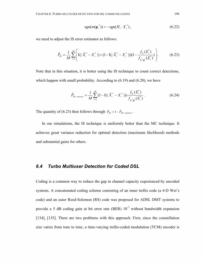
CHAPTER 6. TURBO MULTIUSER DETECTION FOR DSL COMMUNICATIONS 196
* *sgn( ( )) sgn( )i i im H X= − ⋅ρ , (6.22)
we need to adjust the IS error estimator as follows:
* *
** * * *
*1 |
( )1ˆ ˆ ˆ(| |) (1 (| |))(1 )( )
i
i i
ME i
IS i i i ii iE
f EP X X X X
M f E=
= Ι − + − Ι − −
∑ρ
. (6.23)
Note that in this situation, it is better using the IS technique to count correct detections,
which happen with small probability. According to (6.19) and (6.20), we have
* *
** *
*1 |
( )1ˆ ˆ(1 (| |))( )
i
i i
ME i
IS correct i ii iE
f EP X X
M f E−=
= − Ι −∑ρ
. (6.24)
The quantity of (6.23) then follows through correctISIS PP −−= ˆ1ˆ .
In our simulations, the IS technique is uniformly better than the MC technique. It
achieves great variance reduction for optimal detection (maximum likelihood) methods
and substantial gains for others.
6.4 Turbo Multiuser Detection for Coded DSL Coding is a common way to reduce the gap in channel capacity experienced by uncoded
systems. A concatenated coding scheme consisting of an inner trellis code (a 4-D Wei’s
code) and an outer Reed-Solomon (RS) code was proposed for ADSL DMT systems to
provide a 5 dB coding gain at bit error rate (BER) 10-7 without bandwidth expansion
[134], [135]. There are two problems with this approach. First, since the constellation
size varies from tone to tone, a time-varying trellis-coded modulation (TCM) encoder is

CHAPTER 6. TURBO MULTIUSER DETECTION FOR DSL COMMUNICATIONS 197
required. Second, further improvement is very difficult from a practical implementation
perspective because of the complexity of Viterbi decoding for multidimensional TCM.
Recently powerful turbo coding has been proposed for DMT systems [8], [47], [66],
[122]. One typical turbo code is used to code across all subchannels. The coded bits are
then interleaved and allocated to various tones for quadrature amplitude modulation.
Thus, a single standard binary decoder can be employed at the receiver and further
improvement in turbo coding is easily incorporated. A coding gain of 6.0 dB for
bandwidth efficiency of 2 bits/s/Hz and 4.1 dB for 3 bits/s/Hz was reported for a channel
with severe ISI at BER 10-5 [66].
Here we consider the application of turbo multiuser detection in a coded DMT VDSL
system to combat crosstalk and to obtain substantial coding gain. We also consider the
effects of impulse noise, which has been found to greatly impact the performance of our
proposed receiver, and an erasure decoding technique is proposed as a remedy.
De-INT
SISODEC
INT
+
+
−
−
)( ,1 ikbΛ
)(2 jbΛ
)( ,1 ikbλ
)(2 jbλ
Soft Metric Calc.
1 ( )pjbλ
2 ,( )pk ibλ
De-INT
SISODEC
INT
+
+
−
−
)( ,1 ikbΛ
)(2 jbΛ
)( ,1 ikbλ
)(2 jbλ
Soft Metric Calc.
De-INT
SISODEC
INT
+
+
−
−
)( ,1 ikbΛ
)(2 jbΛ
)( ,1 ikbλ
)(2 jbλ
Soft Metric Calc.
1 ( )pjbλ
2 ,( )pk ibλ
Fig. 6.3 Turbo structure for iterative demodulation and decoding
Figure 6.3 shows the turbo structure for iterative demodulation and decoding. It consists
of two stages: a soft metric calculator (the demodulation stage) and a SISO channel
decoder (the decoding stage). The two stages are separated by an interleaver and a de-

CHAPTER 6. TURBO MULTIUSER DETECTION FOR DSL COMMUNICATIONS 198
interleaver. The crosstalk signals are first detected via a multiuser detection technique,
discussed in the last subsection. Then a channel log-likelihood ratio for the kth bit carried
by the ith subchannel symbol is calculated as follows:
,1 ,
,
( 1| ( ))( ) log
( 1| ( ))k i
k ik i
P b r tb
P b r t=
Λ == −
, (6.25)
where r(t) is the received waveform as shown in Fig. 6.1(c). Using Bayes’ formula and
discarding the common term ( ( ))p r t , (6.25) can be written as
1 , 2 ,
, ,1 ,
, ,
( ) ( )
( ( ) | 1) ( 1)( ) log log
( ( ) | 1) ( 1)p
k i k i
k i k ik i
k i k i
b b
p r t b P bb
p r t b P bλ λ
= =Λ = +
= − = −, (6.26)
where the second term 2 ,( )pk ibλ represents the a priori LLR delivered from the decoding
stage in the previous iteration. For the first iteration, this term is set to zero if we assume
equally likely coded bits. The first term 1 ,( )k ibλ , denoting the extrinsic information
obtained from the demodulation stage about the bit ,k ib , is then de-interleaved and sent to
the channel decoder as its a priori information. Similarly, the SISO channel decoder
computes the a posteriori LLR of each code bit and then excludes the influence of a
priori knowledge to get extrinsic information from the decoding stage about the bit
jb (the de-interleaved version of ,k ib , alternatively the coded bits before the interleaver in
Fig. 6.1(a)) as follows:
2 2 1 1
( 1| decoding)( ) ( ) ( ) log ( )
( 1| decoding)jp p
j j j jj
P bb b b b
P bλ λ λ
== Λ − = −
= −. (6.27)

CHAPTER 6. TURBO MULTIUSER DETECTION FOR DSL COMMUNICATIONS 199
Again, this extrinsic information is interleaved and fed back to the demodulation stage as
a priori knowledge for the next iteration. At the last iteration, the SISO decoder also
computes the a posteriori LLRs for information bits, which are used to make final
decisions. More details on this turbo decoding process is given in the following.
6.4.1 Turbo Decoding for Coded DMT System In contrast to trellis-coded modulation where coding and modulation are considered
jointly to obtain an optimal signal constellation in the sense of maximum Euclidean
distance in the signal space, the iterative decoding process we propose separates
demodulation and channel decoding stages for ease of implementation. The greatest
benefits of this turbo process are the very large increase in code memory due to the
interleaver, and almost no loss of optimality due to the iterative exchange of extrinsic soft
information.
Assuming the independence of the background noise between subchannels and
between the two dimensions of each subchannel, the soft metric delivered by the
demodulation stage (see (6.26)) can be expressed as
,1 ,
,
,
,
, ,
, ,
( ( ) | 1)( ) log
( ( ) | 1)( | 1)
log( | 1)( , 1) ( 1)
log( , 1) ( 1)
k ik i
k i
i k i
i k i
i k i k i
i k i k i
p r t bb
p r t bp Y b
p Y bp Y b P bp Y b P b
λ=
== −
==
= −
= = −=
= − =

CHAPTER 6. TURBO MULTIUSER DETECTION FOR DSL COMMUNICATIONS 200
,
,
,
,
,
,: 1
,: 1
,: 1
,: 1
, 2 ,. : 1
, 2
( , ) ( 1)log
( , ) ( 1)
( | ) ( ) ( 1)log
( | ) ( ) ( 1)
ˆ( | , ) ( )log ˆ( | , )
i k i
i k i
i k i
i k i
i k i
i i k ib
i i k ib
i i i k ib
i i i k ib
Mi i i m m l i
X b l k
Mi i i m m
p Y P b
p Y P b
p Y P P b
p Y P P b
p Y X C P b
p Y X C
=
=−
=
=−
== ≠
=
⋅ = −
=⋅ =
⋅ = −
=⋅ =
=
∑
∑
∑
∑
∑ ∏
b
b
b
b
b
b
b b
b b
,
,: 1
.( )
i k i
l iX b l k
P b=− ≠
∑ ∏
(6.28)
Here the second equality holds as 1( , , )TNY Y=Y … is a sufficient statistic for ( )r t and
has independent components. The third equality comes from Bayes’ formula. The iL
different bits 1, , , , ii i L ib b=b assigned to a symbol iX can be modeled as being
independent due to the interleaving effect, which leads to the last equality, where the
summations are over all possible DMT symbol realizations with the indicated conditions.
Note that, to be exact, the marginal distribution for the crosstalk signals should be
incorporated in the last equality of (6.28). But this unrealistic approach would hinder the
implementation of the proposed algorithm in practice. Instead, we use the MUD schemes
discussed in 6.3 to detect the crosstalk signals first and subtract them from the received
signal. For ML-MUD, the crosstalk signals are detected and subtracted from the received
signal before iteration begins. As we can see, ML-MUD makes a thorough search over
the product space spanned by the desired VDSL DMT signal and the crosstalk signals, so
the refined estimates from the decoding stage for the data bits would not help here.
However, for IC-MUD, after each iteration, the LLRs from the SISO decoder are used to
help better detect the crosstalk signals, and ultimately obtain a better estimate of the code

CHAPTER 6. TURBO MULTIUSER DETECTION FOR DSL COMMUNICATIONS 201
bits at the soft metric calculator (see step 1 of the IC-MUD scheme in 6.3.2). For the last
expression in (6.28), we have the formula
, , 2 ,1( ) [1 tanh( ( ))]2
pk i k i k iP b b bλ= + , (6.29)
where 2 ,( )pk ibλ represents the corresponding a priori LLR delivered from the channel
decoding stage in the previous iteration. Invoking the Gaussian assumption on the
background noise, we can also write
2
, ,22
ˆ
2, 2 2
1ˆ( | , )2
M
i i i i m i mm
Y H X F C
Mi i i m mp Y X C e σ
πσ
=
− ⋅ − ⋅
−
=
∑
= , (6.30)
where 2σ is the noise variance per dimension. Due to the independence of the in-phase
and quadrature data, the above formulas (6.28) through (6.30) can be treated for each
dimension separately.
For the channel decoding stage, algorithms discussed in 4.3.2 can be used and details
are ignored here.
6.5 Numerical Results
6.5.1 Robust Multiuser Detection with Impulse Noise In this subsection we examine the behavior and the performance of the proposed
multiuser detection receivers for DMT-VDSL signals with crosstalk and impulse noise

CHAPTER 6. TURBO MULTIUSER DETECTION FOR DSL COMMUNICATIONS 202
via computer simulations. Bit-error-rate (BER) is adopted as the performance measure
with respect to the average signal-to-noise ratio (SNR), which is defined as
2
1
2
1
.
N
i ii
N
ii
H X
E
=
=
⋅=∑
∑SNR (6.31)
In the simulation, the DMT VDSL signal is assumed to occupy 0-25.6 MHz with 256
subchannels in an frequency-division multiplexed (FDM) design. The symbol rate for
each VDSL subchannel is 100 kHz. In each subchannel, 2 bits are assigned so the signals
are 4-QAM. No bit allocation algorithms are used here, although extension to this case is
straightforward. The transfer function of the DMT VDSL signal is simulated by
2
32
2 4 2( ) 100.965 1.50 0.539
j jj
j j
e eH ee e
ω ωω
ω ω
− −−
− −
− −= ×
− +. (6.32)
We assume one NEXT crosstalk signal with a known coupling function given as
3/ 4( )jF e Kω ω= ⋅ , (6.33)
where K is a constant used to adjust the PSD of the crosstalk signal. These settings are
made to roughly approach the PSD shapes indicated in [10]. We assume that these
transfer functions stay fixed for the whole simulation interval, which is reasonable for
wireline communications environments. The crosstalk signal is BPSK modulated on 8
MHz carrier frequency with a 1M symbol-per-second rate. Such a situation would arise,
for example, due to the coexistence of home-phone LANs and asymmetric DMT VDSL
signals in the same cable in the customer premises [16], [17], [18]. Thus, there are 210
possible crosstalk sequences in one VDSL symbol. This number is chosen for simulation
simplicity. In reality, this number could be much larger. The impulse noise is assumed to

CHAPTER 6. TURBO MULTIUSER DETECTION FOR DSL COMMUNICATIONS 203
have parameters 0.1ε = and 100κ = , which means the impulse spike is 20 dB higher
than the background noise floor. The average PSD levels of the crosstalk signal and
background noise floor are fixed while that of the desired signal is varied, corresponding
to different line lengths (the signal attenuation is increasing with the line length). In our
simulation, the average PSD of the crosstalk is 27 dB higher than that of the background
noise floor and the peak PSD of the crosstalk is 40 dB higher. These settings seem to
agree roughly with empirical measurements.
12 13 14 15 16 17 18 19 20 21 22 2310
-7
10-6
10-5
10-4
10-3
10-2
10-1
SNR
BE
R
Fig. 6.4 Bit error rate (BER) versus signal-to-noise ratio (SNR) for different detectors (x-mark: SUD, circle: IC-MUD, diamond: ML-MUD, dashed: single user lower bound)
Figure 6.4 shows the performance of various detectors for DMT VDSL systems with
one crosstalker and impulse noise. As we can see, there is a significant gap between the
performance of the traditional single user detector and the single user lower bound
(corresponding to a crosstalk-free channel), indicating the ineffectiveness of the single-
user detector. While the maximum likelihood multiuser detector essentially achieves the

CHAPTER 6. TURBO MULTIUSER DETECTION FOR DSL COMMUNICATIONS 204
single user lower bound, it suffers from prohibitive complexity. The interference
cancellation multiuser detector offers a favorable performance and complexity tradeoff
compared with the single-user and ML multiuser detectors.
12 13 14 15 16 17 18 19 20 21 22 2310
-7
10-6
10-5
10-4
10-3
10-2
10-1
SNR
BE
R
Fig. 6.5 Bit error rate (BER) versus signal-to-noise ratio (SNR) for different detectors (x-mark: SUD, circle: IC-MUD, plus: IC-MUD-R, diamond: ML-MUD, star: ML-MUD-R, dashed: single user lower bound). Figure 6.5 shows the performance of the M-estimator-based robust detectors in the
crosstalk and impulse noise environment. While there is not much difference between the
ML multiuser detector and its robust version, both of which approximate the single user
lower bound, there is significant improvement for the robust interference cancellation
multiuser detection compared with its Gaussian-based counterpart. The crosstalk
detection errors are 43.42 10−× for IC-MUD, 56.10 10−× for IC-MUD-R and almost 0 for
ML-MUD and ML-MUD-R. It should be noted that the expected improvement from
using M-estimators is due to better estimation of the crosstalk signals in the DMT VDSL

CHAPTER 6. TURBO MULTIUSER DETECTION FOR DSL COMMUNICATIONS 205
case. The desired DMT VDSL signals in different subchannels are independent while the
crosstalk signals are correlated in the frequency domain, which means that M-estimators
are especially applicable to impulse-noise-contaminated DMT VDSL systems with
crosstalk signals strongly correlated in the frequency domain.
6.5.2 Turbo Multiuser Detection In this subsection we examine the behavior and the performance of the proposed turbo
multiuser detection receivers for coded DMT-VDSL signals with crosstalk via computer
simulations. The main results are with an AWGN channel, although impulse noise issues
are also addressed briefly. BER is adopted as the performance measure with respect to
the geometric SNR, which is defined as
1/
1
SNRSNR (1 ) 1 ,NN
igeo
i=
= Γ ⋅ + − Γ ∏ (6.34)
where SNR i is the SNR on the ith subchannel, and Γ is the SNR gap to capacity [22]
which is defined as
2min
23 ,4dσ
⋅Γ = (6.35)
where as before 2σ is the ambient noise variance per dimension, which is assumed the
same for all subchannels, and mind is the minimum Euclidean distance of the received
signals, which is also assumed to be the same for all used subchannels. The rationale for
achieving the same gap for all used subchannels is that the aggregate performance is
approximately maximized if the BERs in all used subchannels are equal. Note that

CHAPTER 6. TURBO MULTIUSER DETECTION FOR DSL COMMUNICATIONS 206
2 2 2min | | , 1i id d H i N= ≤ ≤ , (6.36)
where id is constellation point distance for the ith subchannel. Assuming that the ith
subchannel carries ic bits of information using 2 icM = QAM modulation, we have
2SNRlog 1 .i
ic = + Γ (6.37)
Then the total number of bits transmitted in one DMT symbol is given by
2 2SNRlog 1 log 1 .geoi
ii i
SNRc c N = = + = ⋅ + Γ Γ ∑ ∑ (6.38)
Thus, the geometric SNR allows a direct comparison of performance for all single and
multicarrier systems with the same bit rate cN
. The SNRs used in this simulation are
measured as 0
bEN
, the energy per information bit divided by the one-sided noise power
spectral density ( 20 2N σ= ).
In the simulations, the DMT VDSL signal is assumed to occupy 0-25.6 MHz with
256 subchannels in a FDM design. The symbol rate for each VDSL subchannel is 100
kHz. A rate-1/2 convolutional code with constraint length 5 and generator polynomials
[23, 35]8 is used for channel coding. The number of coded bits per data frame is set as
1024, indicating an average bit rate of 512 bits per DMT block or 2 bits/s/Hz. A random
interleaver of length 1024 is used for interleaving and de-interleaving. The coded DMT
system is applied to a channel with severe ISI, the transfer function of which is taken
from [66] to be
( ) 1 0.9cos( )H Tω ω= + . (6.39)

CHAPTER 6. TURBO MULTIUSER DETECTION FOR DSL COMMUNICATIONS 207
This channel is not necessarily typical of a VDSL line transfer function, however it
serves as a useful example for illustration purposes. Campello’s margin-adaptive bit-
loading algorithm [14] is used to allocate bits to DMT subchannels. We assume a square
QAM constellation for simplicity, so the granularity of bit loading equals 2. Also the first
two tones (up to 200 KHz) are not used for compatibility with POTS/ISDN service.
Figure 6.6 gives the bit allocation used for our simulation. We see that typical
constellations are 64-, 16- and 4-QAM. Subchannels not able to transmit 2 bits reliably
are not used.
50 100 150 200 2500
1
2
3Bit allocation
Subchannel i
bits
per
dim
ensi
on
Fig. 6.6 Bit allocation for DMT subchannels
We assume one NEXT crosstalk signal with a known coupling function. The
crosstalk signal is binary phase-shift keying (BPSK) modulated, carried on a 12.8 MHz
central frequency with a 0.8M symbol-per-second rate. The average PSD of the crosstalk

CHAPTER 6. TURBO MULTIUSER DETECTION FOR DSL COMMUNICATIONS 208
1 2 3 4 5 6 7 810
-7
10-6
10-5
10-4
10-3
10-2
10-1
100 ML-MAP
Geometric SNR (dB)
Bit
Erro
r Rat
e
1st iteration2nd iteration3rd iteration4th iteration5th iteration
Fig. 6.7 Performance of the ML-MAP turbo multiuser receiver
1 2 3 4 5 6 7 810
-7
10-6
10-5
10-4
10-3
10-2
10-1
100 IC-MAP
Geometric SNR (dB)
Bit
Erro
r Rat
e
1st iteration2nd iteration3rd iteration4th iteration5th iteration
Fig. 6.8 Performance of the IC-MAP turbo multiuser receiver

CHAPTER 6. TURBO MULTIUSER DETECTION FOR DSL COMMUNICATIONS 209
1 2 3 4 5 6 7 810
-7
10-6
10-5
10-4
10-3
10-2
10-1
100 ML-SOVA
Geometric SNR (dB)
Bit
Erro
r Rat
e
1st iteration 2nd iteration3rd iteration4th iteration5th iteration
Fig. 6.9 Performance of the ML-SOVA turbo multiuser receiver
1 2 3 4 5 6 7 810
-7
10-6
10-5
10-4
10-3
10-2
10-1
100 IC-SOVA
Geometric SNR (dB)
Bit
Erro
r Rat
e
1st iteration 2nd iteration3rd iteration4th iteration5th iteration
Fig. 6.10 Performance of the IC-SOVA turbo multiuser receiver

CHAPTER 6. TURBO MULTIUSER DETECTION FOR DSL COMMUNICATIONS 210
is 30 dB higher than that of the background noise floor, and the peak PSD of the crosstalk
is 48 dB higher.
Figures 6.7 to 6.10 give, respectively, the performance for the first five iterations for
four different receivers exploiting either ML or IC for MUD detection, and MAP or
SOVA for channel decoding. These receivers are called ML-MAP, IC-MAP, ML-SOVA
and IC-SOVA. From these figures, we see that turbo processing monotonically improves
the system performance, with large gain obtained in a few iterations. We also observe
that the IC-MUD scheme, incorporated into the turbo process, performs as well as the
ML-MUD scheme does with much lower computational requirements. However, IC-
MUD is sub-optimal when used to combat crosstalk signals alone, which we will see
shortly. Finally, SOVA decoding performs almost as well as MAP, with only a few tenths
of a dB loss, but with the advantage of much lower complexity.
To get an overall idea of how much gain is obtained through turbo multiuser detection
of a coded DMT system, we compare the performance of the proposed schemes with
their SUD, uncoded and non-iterative counterparts in Fig. 6.11. Here, SUD means
application of traditional demodulation to the uncoded DMT system, while IC-MUD and
ML-MUD mean application of the corresponding multiuser detection scheme on an
uncoded system. Clearly, MUD greatly outperforms SUD. For BER greater than 310− ,
IC-MUD performs identically with ML-MUD. But when the desired signal level
increases, the performance of IC diminishes. (It is well known that IC performs worst
when the powers of the different users are equal or comparable.) IC-MUD+VA and ML-
MUD+VA refer to detection of a coded DMT VDSL signal in a non-iterative way: after
multiuser detection, hard decisions are made on coded bits, then the Viterbi algorithm is

CHAPTER 6. TURBO MULTIUSER DETECTION FOR DSL COMMUNICATIONS 211
used for decoding. The coded DMT system has a smaller mind compared with its
uncoded counterpart for the same 0
bEN
, but the coding gain more than offsets this
disadvantage. We see that at BER 710− , ML-MUD+VA provides 2.5 dB gain over ML-
MUD. Again, the IC-MUD+VA scheme deteriorates for higher DMT signal levels. The
ML-MUD+MAP and IC-MUD+SOVA denote the performance of our turbo iterative
algorithms, ML-MAP and IC-SOVA, at the fifth iteration. At BER 710− , we see that an
additional 4.5 dB gain is achieved over ML-MUD+VA.
0 1 2 3 4 5 6 7 8 9 10 11 12 13 14 1510
-7
10-6
10-5
10-4
10-3
10-2
10-1
100 Performance Comparison
Geometric SNR (dB)
Bit
Erro
r Rat
e
SUD IC-MUD ML-MUD IC-MUD+VA ML-MUD+VA ML-MUD+MAP IC-MUD+SOVASUD+MAP
Fig. 6.11 Performance comparison of various DMT VDSL receivers
For completeness, we include the performance of SUD+MAP, which means the turbo
iterative decoder (with MAP algorithm for channel decoding) without the MUD
processing step (either ML-MUD or IC-MUD), at the fifth iteration. It can be seen from
the figure that, without multiuser detection, the received signal is crosstalk-dominated

CHAPTER 6. TURBO MULTIUSER DETECTION FOR DSL COMMUNICATIONS 212
and the turbo decoding process is useless. We have also examined the performance of the
turbo iterative receiver when the IC-MUD is executed only once at the first iteration and
found the performance is identical with our proposed receiver which incorporates the IC-
MUD in the iterative process. In other words, in our settings one-time IC-MUD is
enough. That is because in the BER range of interest, the power level of the desired
VDSL signal is so small compared to that of the dominant NEXT, so the IC scheme has
excellent performance here. Nonetheless, we incorporate the IC-MUD in the turbo
process in our proposed scheme for generality and believe it will help in other situations.
In the following, we further address two related issues for our proposed iterative
DMT receiver. For simplicity, we do not include crosstalk signals (thus no need for MUD
in the SISO demodulation stage) and MAP is used in the SISO decoder. Usually in
multilevel QAM symbol mapping, Gray coding is used so that a symbol detection error
results in only one bit error. For our proposed iterative decoding process, we found that
natural coding actually outperforms Gray coding. Figures 6.12 and 6.13 give the
performance of the iterative DMT receiver with Gray coding and natural coding for first
five iterations. It is shown that with Gray coding, the receiver is saturated after two
iterations with performance worse than natural coding.
This phenomenon can be attributed to the reduced minimum Euclidian distance
associated with Gray symbol mapping. Consider, for example, a one-dimension signal
level of 16-QAM. Figures 6.14 and 6.15 show Gray coding and natural coding for a 4-
PAM constellation. In our proposed scheme, the demodulation stage yields a soft metric
for each coded bit based on the received noise-contaminated signal and a priori
information of all other bits of the same DMT symbol from the decoding stage. Let us

CHAPTER 6. TURBO MULTIUSER DETECTION FOR DSL COMMUNICATIONS 213
1 2 3 4 5 6 7 810
-7
10-6
10-5
10-4
10-3
10-2
10-1 Gray Coding
Geometric SNR (dB)
Bit
Erro
r Rat
e
1st iteration2nd iteration3rd iteration4th iteration5th iteration
Fig. 6.12 Performance of the iterative DMT receiver with Gray coding
1 2 3 4 5 6 7 810
-7
10-6
10-5
10-4
10-3
10-2
10-1
100 Natural Coding
Geometric SNR (dB)
Bit
Erro
r Rat
e
1st iteration2nd iteration3rd iteration4th iteration5th iteration
Fig. 6.13 Performance of the iterative DMT receiver with natural coding
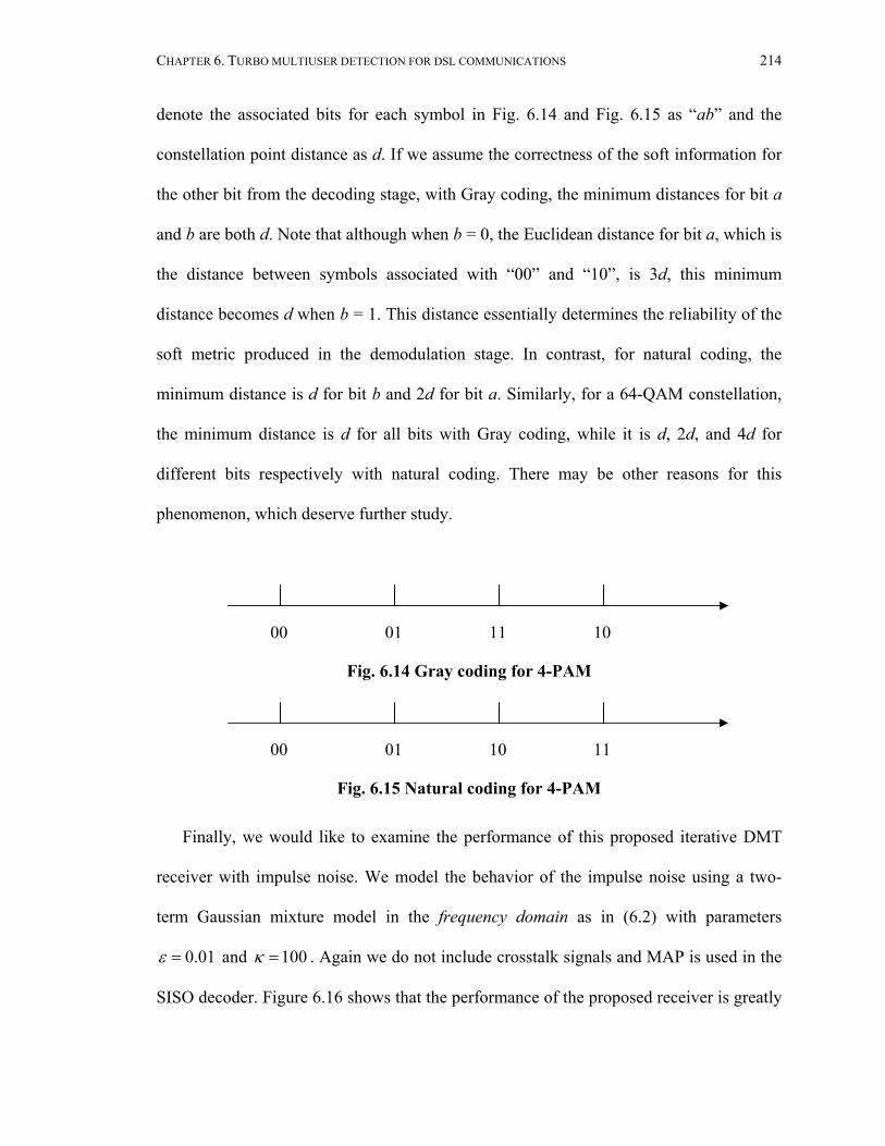
CHAPTER 6. TURBO MULTIUSER DETECTION FOR DSL COMMUNICATIONS 214
denote the associated bits for each symbol in Fig. 6.14 and Fig. 6.15 as “ab” and the
constellation point distance as d. If we assume the correctness of the soft information for
the other bit from the decoding stage, with Gray coding, the minimum distances for bit a
and b are both d. Note that although when b = 0, the Euclidean distance for bit a, which is
the distance between symbols associated with “00” and “10”, is 3d, this minimum
distance becomes d when b = 1. This distance essentially determines the reliability of the
soft metric produced in the demodulation stage. In contrast, for natural coding, the
minimum distance is d for bit b and 2d for bit a. Similarly, for a 64-QAM constellation,
the minimum distance is d for all bits with Gray coding, while it is d, 2d, and 4d for
different bits respectively with natural coding. There may be other reasons for this
phenomenon, which deserve further study.
Fig. 6.14 Gray coding for 4-PAM
Fig. 6.15 Natural coding for 4-PAM
Finally, we would like to examine the performance of this proposed iterative DMT
receiver with impulse noise. We model the behavior of the impulse noise using a two-
term Gaussian mixture model in the frequency domain as in (6.2) with parameters
0.01ε = and 100κ = . Again we do not include crosstalk signals and MAP is used in the
SISO decoder. Figure 6.16 shows that the performance of the proposed receiver is greatly
00 01 11 10
00 01 10 11

CHAPTER 6. TURBO MULTIUSER DETECTION FOR DSL COMMUNICATIONS 215
degraded with impulse noise. The use of erasure decoding can remedy this. In the
demodulation stage, for those bits associated with impulse-contaminated symbols, instead
of calculating soft metrics for them, the a priori information is used as a substitute, i.e.,
1 , 2 ,( ) ( )pk i k ib bλ λ= . (For the first iteration, these are set to zeros.) In DMT systems, the
erasure positions where impulse spikes appear can possibly be detected in advance
through pilot tones. In Fig. 6.17, we see that the performance of the proposed receiver
experiences almost no performance loss with impulse noise with the aid of erasure
decoding.
1 2 3 4 5 6 7 810
-7
10-6
10-5
10-4
10-3
10-2
10-1
100 Impulse Noise
Geometric SNR (dB)
Bit
Erro
r Rat
e
1st iteration2nd iteration3rd iteration4th iteration5th iteration
Fig. 6.16 Performance of the iterative DMT receiver with impulse noise

CHAPTER 6. TURBO MULTIUSER DETECTION FOR DSL COMMUNICATIONS 216
1 2 3 4 5 6 7 810
-7
10-6
10-5
10-4
10-3
10-2
10-1
100 Impulse Noise with Erasure Decoding
Geometric SNR (dB)
Bit
Erro
r Rat
e
1st iteration2nd iteration3rd iteration4th iteration5th iteration
Fig. 6.17 Performance of the iterative DMT receiver with erasure decoding with
impulse noise
6.6 Summary In this chapter we have shown the potential benefits of multiuser detection for crosstalk
mitigation in DMT VDSL systems subject to impulse noise. We see that ML-MUD can
essentially eliminate crosstalk signals in DMT systems at a cost of high complexity. As a
tradeoff, IC-MUD can significantly outperform SUD, with lower complexity than ML-
MUD. We have also shown the effectiveness of the M-estimator in combating the
impulse noise.
Further, a new coded DMT VDSL receiver structure using turbo multiuser detection
has been proposed and has been shown to achieve an overall 7.0 dB gain over the
uncoded optimum (maximum likelihood) receiver at BER 710− for a channel with severe
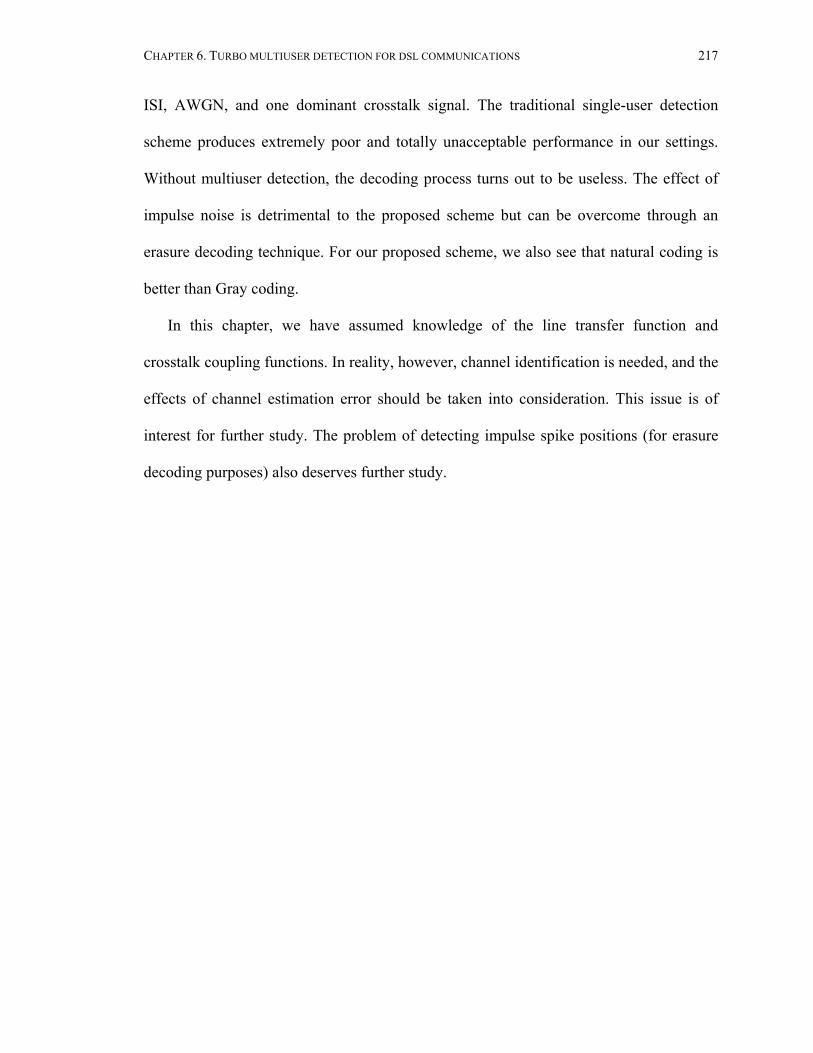
CHAPTER 6. TURBO MULTIUSER DETECTION FOR DSL COMMUNICATIONS 217
ISI, AWGN, and one dominant crosstalk signal. The traditional single-user detection
scheme produces extremely poor and totally unacceptable performance in our settings.
Without multiuser detection, the decoding process turns out to be useless. The effect of
impulse noise is detrimental to the proposed scheme but can be overcome through an
erasure decoding technique. For our proposed scheme, we also see that natural coding is
better than Gray coding.
In this chapter, we have assumed knowledge of the line transfer function and
crosstalk coupling functions. In reality, however, channel identification is needed, and the
effects of channel estimation error should be taken into consideration. This issue is of
interest for further study. The problem of detecting impulse spike positions (for erasure
decoding purposes) also deserves further study.

218
Chapter 7
Conclusions and Perspectives In this dissertation, both signal processing and information theoretic aspects of wireless
cellular communications with antenna arrays have been studied. Specifically, we have
investigated various transmit diversity and downlink beamforming techniques with power
control for wireless cellular communications with transmit arrays, and iterative space-
time multiuser detection techniques with receive arrays. Further, turbo space-time
multiuser detection has been employed for wireless cellular MIMO communications.
Then, for the multicell MIMO systems where co-channel interference is the dominating
detrimental factor, various multiuser receivers have been proposed to dramatically
improve the system performance. Spectral efficiencies of these receivers have been
analyzed, together with their large-system asymptotic (non-random) expressions. The
turbo multiuser detection techniques have also been applied to the DSL wireline
communications to effectively combat the crosstalk, with the influence of impulse noise
taken into consideration.
The contributions of this dissertation are summarized in the following.
Chapter 2: It has been shown that traffic type impacts algorithm choice. For circuit-
switched downlink CDMA systems, Max SNR beamforming is the best choice
(accommodates 12 to 42 more users than transmit diversity). For packet-switched
CONCLUSIONS AND PERSPECTIVES 219
systems, Max SINR Beamforming has the best performance in terms of peak rate (10-14
dB more than transmit diversity); Max SNR beamforming is almost the best in terms of
mean rate (3-4 dB more than transmit diversity), but beam steering and transmit diversity
with sectorization are also good choices. It has also been found that sectorization greatly
improves the system performance, both for the circuit and for the packet case. For
transmit diversity, the gain through exploiting more antennas diminishes, while this is not
the case for beamforming techniques, especially with feedback channel parameters.
Chapter 3: For batch iterative methods, it has been shown that fully exploiting
diversities through space-time processing and multiuser detection offers substantial
improvement over alternative processing methods, and that iterative implementation of
these linear and nonlinear multiuser receivers realizes this substantial gain and
approaches the optimum performance with reasonable complexity. Among these iterative
implementations the SAGE space-time multiuser receiver outperforms the others. The
complexity of the new SAGE detector with the traditional structure is no higher than the
existing methods but with better performance and smoother convergence. The SAGE
detector with a new structure retains its excellent performance but with greater
adaptability, and its complexity is comparable to the existing methods. For sample-by-
sample adaptive methods, it is shown that the data aided adaptive space-time multiuser
receivers combine the functions of adaptive beamforming, RAKE combining and
multiuser detection with no side information needed other than the timing and training
sequences of the desired user. The alternative blind adaptive space-time multiuser
receiver is based on the LCMV criterion and min-max parameter estimation. This
detector is robustified against signature waveform mismatch with norm-constrained

CONCLUSIONS AND PERSPECTIVES 220
techniques. LMS implementations of all of these adaptive ST MUD receivers have been
given, and the convergence and excess-MSE issues have been discussed.
Chapter 4: Turbo space-time multiuser detection has been introduced for intracell
wireless MIMO communications. Among various multiuser detection techniques
examined to combat the intercell interference, linear MMSE MUD and successive
interference cancellation have been shown to be feasible and effective. Based on these
two multiuser detection schemes, one of which may outperform the other for different
settings, an adaptive detection scheme has been developed, which together with a Turbo-
BLAST structure offers substantial performance gain over the well known V-BLAST
techniques with coding in this interference-limited cellular environment. The obtained
multiuser capacity is excellent in high to medium SIR scenario. Nonetheless, numerical
results also indicate that a further increase in system complexity, using base-station
cooperation, could lead to further significant increases of the system capacity.
Chapter 5: The spectral efficiency of the multicell MIMO systems with several
MUD detectors has been studied, among which are single-cell detectors, joint optimum
detectors, group linear MMSE detectors, group MMSE successive cancellation detectors,
and adaptive multiuser detectors. The large-system asymptotic (non-random) expressions
for these spectral efficiencies are also explored. As applications of these theoretical
bounds, we have verified the following observations of Chapter 4 about multicell MIMO
systems. Group linear MMSE detection and group MMSE successive cancellation are
two effective techniques to combat the co-channel interference, each of which may
outperform the other for different settings. For full system load, multiuser detection
across the cell is most useful in strong interference environments, offering substantial

CONCLUSIONS AND PERSPECTIVES 221
gain over traditional single-cell detectors. However, there is still a substantial gap
between the achievable capacity and the single cell upper bound in this case. Further, the
conditions for non-interference-limited behavior of the group linear MMSE detector have
been found. Based on this result, it is suggested that with sufficiently low system load
11L
β ≤+
, where L is the number of effective interfering cells, a better performance than
the fully loaded system may be attained in the strong interference environment with
sufficiently large signal power. If the interference is weak, then a high-load system with
fairly simple group linear MMSE detection has the advantage.
Chapter 6: The potential benefits of multiuser detection for crosstalk mitigation in
DMT VDSL systems have been shown. ML-MUD can essentially eliminate crosstalk
signals in DMT systems at a cost of high complexity. As a tradeoff, IC-MUD can
significantly outperform single-user detection, with lower complexity than ML-MUD.
The effectiveness of the M-estimator in combating the impulse noise has also been
shown. Further, a new coded DMT VDSL receiver structure using turbo multiuser
detection has been proposed and has been shown to achieve an overall 7.0 dB gain over
the uncoded optimum (maximum likelihood) receiver at BER 710− for a channel with
severe ISI, AWGN, and one dominant crosstalk signal. The detrimental effect of impulse
noise can be overcome through an erasure decoding technique.
Several considerations for future work are now in order.
• As has been shown in Chapters 4 and 5, there is still a remarkable gap
between the achievable capacity and the single cell upper bound with strong co-
channel interference. Therefore, it is worth exploring the cooperation of base

CONCLUSIONS AND PERSPECTIVES 222
stations and the feedback of channel information to enhance the system capacity
in this case. Several promising techniques of interest are: joint transmission [6],
ranked known interference [97], and joint transmit and receive optimization [91].
• The capacity of the whole downlink cellular system, when modeled as a
broadcast/interference channel, has long been an open question. Work on
multiuser information theory in the context of multicell cellular communication
systems is also of interest.
• Besides the physical layer processing focused in this dissertation, the study of
MAC and network layers, and opportunities for cooperation between these layers
and the physical layer in the context of wireless LAN IEEE 802.11, is of interest.
So is the potential for interdisciplinary collaboration in fields such as vehicle
transportation, multimedia communications, and deep-space communications.

223
Bibliography [1] M. Abdulrahman, et al., “Decision feedback equalization for CDMA in indoor
wireless communications,” IEEE J. Select. Areas Commun., vol. 12, no. 4, pp. 698-707, May 1994.
[2] S. L. Ariyavisitakul, “Turbo space-time processing to improve wireless channel capacity,” IEEE Trans. Commun., vol. 48, no. 8, pp. 1347-1359, Aug. 2000.
[3] T. Aste et al, “Downlink beamforming avoiding DOA estimation for cellular mobile communications,” Proc. 1998 IEEE Int. Conf. Acoust. Speech, Sig. Process., pp. 3313-3316, Seattle, Washington, May 1998.
[4] P. D. Alexander, et al., “Iterative multiuser interference reduction: turbo CDMA,” IEEE Trans. Commun., vol. 47, no. 7, pp. 1008-1014, July 1999.
[5] L. R. Bahl et al., “Optimal decoding of linear codes for minimizing symbol error rate,” IEEE Trans. Inform. Theory, vol. IT-20, pp. 284-287, Mar. 1974.
[6] P. W. Baier, M. Meurer, T. Weber and H. Troeger, “Joint transmission (JT), an alternative rationale for the downlink of time division CDMA using multi-element transmit antennas,” Proc. 2000 IEEE 6th Int. Symp. Spread Spectrum Techniques, vol. 1, pp. 1-5, Parsippany, NJ, Sept. 2000.
[7] S. Beheshti and G. W. Wornell, “Joint intersymbol and multiple-access interference suppression algorithms for CDMA systems,” European Trans. Telecomm., vol. 9, no. 5, pp. 403-418, Sept.-Oct., 1998.
[8] C. Berrou et al., “Near shannon limit error-correction coding and decoding: Turbo codes,” Proc. 1993 IEEE International Conf. on Communications, pp. 1064-1070, Geneva, Switzerland, May 1993.
[9] E. Biglieri, J. Proakis, and S. Shamai, “Fading channels: information-theoretic and communications aspect,” IEEE Trans. Inform. Theory, vol. 44, no. 6, pp. 2619-2692, Oct. 1998.
[10] J. Bingham, “Synchronous DMT for low-complexity VDSL,” ANSI T1E1.4/96-081, 1996.
[11] A. Boariu and R. E. Ziemer, “Cholesky-iterative detector: a new multiuser detector for synchronous CDMA systems,” IEEE Commun. Lett., vol. 4, no. 3, Mar. 2000.

BIBLIOGRAPHY 224
[12] R. S. Blum, J. H. Winters, and N. Sollenberger, “On the capacity of cellular systems with MIMO,” Proc. 2001 Fall IEEE Vehicular Technology Conf., CDROM, Atlantic City, NJ, Oct. 2001.
[13] R. Calderbank, “The art of signaling: fifty years of coding theory,” IEEE Trans. Inform. Theory, vol. 44, no. 6, pp. 2561-2595, Oct. 1998.
[14] J. Campello, “Practical bit loading for DMT,” Proc. 1999 IEEE International Conf. on Communications, pp. 801-805, Vancouver, Canada, June 1999.
[15] S. Catreux, P. F. Driessen and L. J. Greenstein, “Simulation results for an interference-limited multiple-input multiple-output cellular system,” IEEE Comm. Lett., vol. 4, no. 11, pp. 334-336, Nov. 2000.
[16] K. W. Cheong and J. M. Cioffi, “Coexistence of 1 Mbps HPNA and DMT VDSL via multiuser detection and code division multiplexing,” ANSI T1E1.4/99-120,1999.
[17] K. W. Cheong and J. M. Cioffi, “Coexistence of 2-10 Mbps Home-Phone LANS and DMT VDSL via multiuser detection,” ANSI T1E1.4/99-333, 1999.
[18] K. W. Cheong et al., “Soft cancellation via iterative decoding to mitigate the effect of home-LANs on VDSL,” ANSI T1E1.4/99-333R1, 1999.
[19] Chkeif, et al., “Spatio-temporal blind adaptive multiuser detection,” IEEE Trans. Commun., vol. 48, no. 5, pp. 729-732, May 2000.
[20] W. J. Choi, R. Negi and J. M. Cioffi, “Combined ML and DFE decoding for the V-BLAST System,” Proc. 2000 IEEE International Conf. on Communications, pp. 1243 –1248, New Orleans, LA, June 2000.
[21] J. M. Cioffi, K. Cheong, J. Lauer, and A. Salvekar, “Mitigation of DSL crosstalk via multiuser detection and code-division multiple access,” ANSI T1E1.4/98-253, 1998.
[22] J. M. Cioffi, “A multicarrier primer,” unpublished notes, Stanford University.
[23] J. M. Cioffi, et al., “Very-high –speed digital subscriber lines,” IEEE Commun. Mag., pp. 72-79, Apr. 1999.
[24] J. W. Cook, “Wideband impulse noise survey of the access network,” BT Technical Journal, Vol. 11, No. 3, pp. 155-162, July 1993.
[25] D. J. Costello, Jr., J. Hagenauer, H. Imai and S. B. Wicker, “Application of error control coding,” IEEE Trans. Inform. Theory, vol. 44, no. 6, pp. 2531-2560, Oct. 1998.
BIBLIOGRAPHY 225
[26] T. M. Cover and J. A. Thomas, Elements of Information Theory, New York: Wiley, 1991.
[27] A. Czylwik and T. Matsumoto, “Downlink beamforming for frequency-duplex systems in frequency-selective fading”, Proc. 2000 Spring IEEE Vehicular Technology Conf., pp. 695-699, Tokyo, Japan, May 2000.
[28] S. Davies, et al., “Impulse noise events of relatively long duration,” ANSI T1E1.4/94-120, 1994.
[29] S. Davies, et al., “Australia wideband impulse noise survey data,” ANSI T1E1.4/95-125, 1995.
[30] P. Dempster, et al., “Maximum likelihood from incomplete data via the EM algorithm,” J. Royal Statistical Soc., Ser. B, vol. 39, no. 1, pp. 1-38, 1977.
[31] D. Divsalar, et al., “Improved parallel interference cancellation for CDMA,” IEEE Trans. Commun., vol. 46, no. 2, pp. 258-268, Feb. 1998.
[32] C. Douillard et al., “Iterative correction of intersymbol interference: Turbo-equalization,” European Trans. Telecommun., vol. 6, no. 5, pp. 507-511, Sept.-Oct. 1995.
[33] D. F. Driessen and G. J. Foschini, “On the capacity formula for multiple input-multiple output wireless channels: a geometric interpretation,” IEEE Trans. Commun., vol. 47, no. 2, pp. 173-176, Feb. 1999.
[34] A. Duel-Hallen, “A family of multiuser decision-feedback detectors for asynchronous code-division multiple access channels,” IEEE Trans. Commun., vol. 43, no. 2/3/4, pp. 421-434, Feb./Mar./Apr. 1995.
[35] H. Elders-Boll, et al., “Efficient implementation of linear multiuser detectors for asynchronous CDMA systems by linear interference cancellation,” European Trans. Telecomm., vol. 9, no. 5, pp. 427-437, Sept.-Oct., 1998.
[36] F. R. Farrokhi, G. J. Foschini, A. Lozano and R. A. Valenzuela, “Link-optimal space-time processing with multiple transmit and receive antennas,” IEEE Comm. Lett., vol. 5, no. 3, pp. 85-87, Mar. 2001.
[37] C. Farsakh and J. Nossek, “Spatial covariance based downlink beamforming in an SDMA mobile radio system,” IEEE Trans. Commun., vol. 46, no. 11, pp. 1497-1506, Nov. 1998.
[38] J. A. Fessler and A. O. Hero, “Space-alternating generalized EM algorithm,” IEEE Trans. Signal Processing, vol. 42, no. 10, pp. 2664-2677, Oct. 1994.
[39] G. D. Forney and G. Ungerboeck, “Modulation and coding for linear Gaussian channels,” IEEE Trans. Inform. Theory, vol. 44, no. 6, pp. 2384-2415, Oct. 1998.

BIBLIOGRAPHY 226
[40] G. J. Foschini, “A simplified distributed autonomous power control algorithm and its convergence,” IEEE Trans. Veh. Technol., vol. 42, no. 4, pp. 641-646, Nov. 1993.
[41] G. J. Foschini, “Layered space-time architecture for wireless communication in a fading environment when using multi-element antennas,” Bell Labs Tech. J., vol. 2, no. 2, pp. 41-59, Autumn 1996.
[42] G. J. Foschini and M. J. Gans, “On limits of wireless communications in a fading environment when using multiple antennas,” Wireless Personal Communications, vol. 6, no. 3, pp. 311-335, Mar. 1998.
[43] G. J. Foschini, G. D. Golden, R. A. Valenzuela and P. W. Wolniansky, “Simplified processing for high spectral efficiency wireless communication employing multi-element arrays,” IEEE J. Selected Areas Comm., vol. 17, pp. 1841-1852, 1999.
[44] M. P. C. Fossorier et al., “On the equivalence between SOVA and Max-Log-MAP decodings,” IEEE Commun. Lett., vol. 2, no. 5, May 1998.
[45] R. Gejji, “Forward-link-power control in CDMA cellular systems,” IEEE Trans. Veh. Technol., vol. 41, no. 4, pp. 532-536, Nov. 1992.
[46] S. Grandhi et al, “Centralized power control in cellular radio systems,” IEEE Trans. Veh. Technol., vol. 42, no. 4, pp. 466-468, Nov. 1993.
[47] S. L. Goff et al., “Turbo codes and high spectral efficiency modulation,” Proc.1994 IEEE International Conf. on Communications, pp.645-649, New Orleans, LA, May 1994.
[48] G. H. Golub and C. F. Van Loan, Matrix Computation, The John Hopkins University Press, Baltimore, MD, 1996
[49] J. Grant and P. D. Alexander, “Random sequence multisets for synchronous code-division multiple-access channels,” IEEE Trans. Inform. Theory, vol. 44, no. 7, pp.2832-2836, Nov. 1998.
[50] J. Hagenauer and P. Hoeher, “A Viterbi algorithm with soft-decision outputs and its applications,” Proc. 1989 IEEE Global Telecommunications Conf., pp. 47. 1.1-47. 1.7, Dallas, TX, Nov. 1989.
[51] J. Hagenauer et al., “Iterative decoding of binary block and convolutional codes,” IEEE Trans. Inform. Theory, vol. 42, no. 2, pp. 429-445, Mar. 1996.
[52] S. Hanly and D. Tse, “Power control and capacity of spread spectrum wireless networks,” Automatica 35, pp. 1987-2012, 1999.

BIBLIOGRAPHY 227
[53] S. Haykin, Adaptive Filter Theory, third edition, Englewood Cliffs, NJ: Prentice-Hall, 1996.
[54] B. Hochwald, T. Marzetta and C. Papadias, “A transmitter diversity scheme for CDMA systems based on space-time spreading,” Bell Labs Technical Memorandum, May 1999.
[55] B. Hochwald and T. Marzetta, “Adapting a downlink array from uplink measurements,” Bell Labs Technical Memorandum, Feb. 1999.
[56] M. Honig, U. Madhow and S. Verdú, “Blind adaptive multiuser detection,” IEEE Trans. Inform. Theory, vol. IT-41, pp. 944-960, July 1995.
[57] H. Huang, “Increasing IS-95 downlink capacity with transmit and receive diversity,” Bell Labs Technical Memorandum, Nov. 1997.
[58] P. J. Huber, Robust Statistics, New York: Wiley, 1981.
[59] K. Hugl et al., “Downlink beamforming for frequency division duplex systems,” Proc. 1999 IEEE Global Telecommunications Conf., pp. 2097-2101, Rio de Janeiro, Brazil, Dec. 1999.
[60] D. Jonsson, “Some limit theorems for the eigenvalues of a sample covariance matrix,” J. Multivariate Anal., vol. 12, pp. 1-38, 1982.
[61] M. Juntti, et al., “Iterative implementation of linear multiuser detection for dynamic asynchronous CDMA systems,” IEEE Trans. Commun., vol. 46, no. 4, pp. 503-508, Apr. 1998.
[62] K. J. Kerpez and C. F. Valenti, “Impulse noise testing for ADSL transceivers,” ANSI T1E1.4/93-034, 1993.
[63] M. A. Khalighi et al., “On capacity of Ricean MIMO channels,” Proc. 2001 IEEE 12th International Symposium on Personal, Indoor and Mobile Radio Communications, pp. A150-A154, San Diego, CA, Sep 30-Oct 3. 2001.
[64] A. Lapidoph, “Mismatched decoding and the multiple-access channel,” IEEE Trans. Inform. Theory, vol. 42, no. 6, pp. 1439-1452, Sept. 1996.
[65] A. Lapidoph, “Nearest neighbor decoding for additive non-Gaussian channels,” IEEE Trans. Inform. Theory, vol. 42, pp. 1520-1529, Sept. 1996.
[66] J. P. Lauer and J. M. Cioffi, “Turbo coding for discrete multitone transmission,” Proc. 1998 IEEE Global Telecommunications Conf., pp. 3256-3260, Sydney, Australia, Nov. 1998.
[67] H. Liu and M. D. Zoltowski, “Blind equalization in antenna array CDMA systems,” IEEE Trans. Signal Processing, vol. 45, no. 1, pp. 161-172, Jan. 1997.

BIBLIOGRAPHY 228
[68] P. Luukkanen and P. Zhang, “Comparison of optimum and sub-optimum turbo decoding schemes in 3rd generation cdma200 mobile system,” Proc. 1999 IEEE Wireless Communications and Networking Conf., pp. 437-441, New Orleans, LA, Sept. 1999.
[69] U. Madhow, “Blind adaptive interference suppression for direct-sequence CDMA,” Proceedings of the IEEE, vol. 86, no. 10, pp. 2049-2069, Oct. 1998.
[70] I. Medvedev and V. Tarokh, “A channel-shortening multiuser detector for DS-CDMA systems," Proc. 2001 Spring IEEE Vehicular Technology Conf., pp. 1834-1838, Rhodes, Greece, May 2001.
[71] G. Montalbano et al., “Spatial-temporal array processing for FDD/CDMA/SDMA downlink transmission,” Proc. 1999 Spring IEEE Vehicular Technology Conf., pp. 1910-1914, Amsterdam, Netherlands, Sept. 1999.
[72] S. Miller and S. C. Schwartz, “Integrated spatial-temporal detectors for asynchronous Gaussian multiple access channels,” IEEE Trans. Commun., vol. 43, no. 2/3/4, pp. 396-411, Feb./Mar./Apr. 1995.
[73] S. L. Miller, “Training analysis of adaptive interference suppression for direct-sequence code-division multiple access systems,” IEEE Trans. Commun., vol. 44, no. 4, pp. 488-495, Apr. 1996.
[74] F. Molisch, “Capacity of the uplink of interference-limited MIMO systems”, AT&T Technical Memorandum, in preparation.
[75] L. B. Nelson and H. V. Poor, “Iterative multiuser receivers for CDMA channels: An EM-based approach,” IEEE Trans. Commun., vol. 44, no. 12, pp. 1700-1710, Dec. 1996.
[76] G. Orsak and B. Aazhang, “On the theory of importance sampling applied to the analysis of detection systems,” IEEE Trans. Commun., vol. 37, no. 4, pp. 332-339, Apr. 1989.
[77] G. Orsak and B. Aazhang, “Efficient importance sampling techniques for simulation of multiuser communication systems,” IEEE Trans. Commun., vol. 40, no. 6, pp. 1111-1118, June. 1992.
[78] J. Paulraj and C. B. Papadias, “Space-time processing for wireless communications,” IEEE Signal Processing Mag., pp. 49-82, Nov. 1997.
[79] H. V. Poor, “Turbo multiuser detection: A primer,” Journal of Communications and Networks, vol. 3, no. 3, pp. 196-201, Sept. 2001.
[80] H. V. Poor and S. Verdú, “Probability of error in MMSE multiuser detection,” IEEE Trans. Inform. Theory, vol. 43, pp. 858-871, 1997.

BIBLIOGRAPHY 229
[81] G. Proakis, Digital Communications, McGraw-Hill, New York, 1995.
[82] G. Raleigh et al., “A blind adaptive transmit antenna algorithm for wireless communications,” Proc.1995 IEEE International Conf. on Communications, pp. 1494-1499, Seattle, WA, June 1995.
[83] G. G. Raleigh and J. M. Cioffi, “Spatio-temporal coding for wireless communication,” IEEE Trans. Commun., vol. 46, no. 3, pp. 357-366, Mar.1998.
[84] P. B. Rapajic and B. S. Vucetic, “Adaptive receiver structures for asynchronous CDMA systems,” IEEE J. Select. Areas Commun., vol. 12, no. 4, pp. 685-697, May 1994.
[85] P. B. Rapajic and D. Popescu, “Information capacity of a random signature multiple-input multiple output channel,” IEEE Trans. Commun., vol. 48, no. 8, pp.1245-1248, Aug. 2000.
[86] T. S. Rappaport, Wireless Communications: Principles and Practice, Prentice-Hall PTR, NJ, 1996.
[87] F. Rashid-Farrokhi et al., “Joint optimal power control and beamforming in wireless networks using antenna arrays,” IEEE Trans. Commun., Vol. 46, no. 10, pp. 1313-1324, Oct. 1998.
[88] F. Rashid-Farrokhi et al., “Transmit beamforming and power control for cellular wireless systems,” IEEE Select. Areas Commun., vol. 16, no. 8, pp. 1437-1449, Oct. 1998
[89] K. Rasmussen, T. J. Lim, and A. Johansson, “A matrix-algebraic approach to successive interference cancellation in CDMA,” IEEE Trans. Commun., Vol. 48, pp. 145-151, Jan. 2000.
[90] P. Roberson et al., “A comparison of optimal and sub-optimal MAP decoding algorithms operating in the log domain,” Proc. 1995 IEEE International Conf. on Communications, pp. 1009-1013, Seattle, WA, June 1995.
[91] H. Sampath and A. J. Paulraj, "Joint transmit and receive optimization for high data rate wireless communication using multiple antennas," Proc. 1999 Asilomar Conf. Signals Systems Comp., pp. 215-219, Pacific Grove, CA, Oct. 1999.
[92] P. J. Smith, M. Shafi and H. Gao, “Quick simulation: A review of importance sampling techniques in communications systems,” IEEE J. Select. Areas Commun., vol. 15, no. 4, pp. 597-613, May 1997.
[93] J. B. Schodorf and D. B. Williams, “A constrained optimization approach to multiuser detection,” IEEE Trans. Commun., vol. 45, no. 1, pp. 258-262, Jan. 1997.

BIBLIOGRAPHY 230
[94] J. B. Schodorf and D. B. Williams, “Array processing techniques for multiuser detection,” IEEE Trans. Commun., vol. 45, no. 11, pp. 1375-1378, Nov. 1997.
[95] S. Shamai (Shitz) and S. Verdu, “The impact of frequency-flat fading on the spectral efficiency of CDMA,” IEEE Trans. Inform. Theory, vol. 47, no. 3, pp.1302-1327, May 2001.
[96] S. Shamai and A. Wyner, “Information theoretic considerations for symmetric, cellular multiple-access fading channels – part I and part II,” IEEE Trans. Inform. Theory, vol. 43, no. 6, pp. 1877-1911, Nov. 1997.
[97] S. Shamai and B. M. Zaidel, “Enhancing the cellular downlink capacity via co-processing at the transmission end,” Proc. 2001 Spring IEEE Vehicular Technology Conf., pp. 1745-1749, Rhodes, Greece, May 2001.
[98] M. Sellathurai and S. Haykin, “Further results on diagonal-layered space-time architecture,” Proc. 2001 Spring IEEE Vehicular Technology Conf., pp. 1958-1962, Rhodes, Greece, May 2001.
[99] J. W. Silverstein and Z. D. Bai, “On the empirical distribution of eigenvalues of a class of large dimensional random matrices,” J. Multivariate Anal., vol. 54, no. 2, pp. 175-192, 1995.
[100] J. W. Silverstein, “Strong convergence of the empirical distribution of eigenvalues of large dimensional random matrices,” J. Multivariate Anal., vol. 55, pp. 331-339, 1995.
[101] J. E. Smee and S. C. Schwartz, “Adaptive space-time feedforward/feedback detection for CDMA,” Proc. 1999 IEEE Workshop on Signal Processing Advances in Wireless Communications, pp. 29-33, Annapolis, Maryland, May 1999.
[102] T. Starr, J. M. Cioffi and P. J. Siverman, Understanding Digital Subscriber Line Technology, Prentice Hall, Upper Saddle River, NJ, 1999.
[103] M. Steinbauer and A. F. Molisch (eds.), “Directional channel modeling,” in L. Correia (ed.), Flexible Personalized Wireless Communications, New York: Wiley, 2001.
[104] V. Tarokh et al., “Space-time codes for high data rate wireless communications: performance criterion and code construction,” IEEE Trans. Inform. Theory, vol. 44, no. 2, pp. 744-765, Mar. 1998.
[105] E. Telatar, “Capacity of multi-antenna Gaussian channels,” European Trans. Telecomm., vol. 10, no. 6, pp. 585-595, Nov.-Dec. 1999.
[106] K. Tsatsanis and Z. Xu, “Performance analysis of minimum variance CDMA receivers,” IEEE Trans. Commun., vol. 46, no. 11, pp. 3014-3022, Nov. 1998.
BIBLIOGRAPHY 231
[107] D. Tse and S. Hanly, “Linear multiuser receivers: effective interference, effective bandwidth and user capacity,” IEEE Trans. Inform. Theory, vol. 45, no. 2, pp.641-657, Mar. 1999.
[108] J. W. Tukey, “A survey of sampling from contaminated distributions,” in Contributions to Probability and Statistics (Harold Hotelling Volume), I. Olkin, et al., eds. Stanford University Press: Stanford, CA, 1960.
[109] F. Valenti, K. J. Kerpez and B. Blake, “Analysis of loop and inside wire background noise measured at two New Jersey residential locations,” ANSI T1E1.4/92-227, 1992.
[110] F. Valenti and K. J. Kerpez, “Analysis of wideband noise measurements and implications for signal processing in ADSL systems”, Proc. 1994 IEEE International Conf. on Communications, pp. 826-832, New Orleans, CA, May 1994.
[111] F. Valenti, “Survey plan for characterization of impulse noise and background noise at VDSL frequencies,” ANSI T1E1.4/97-295, 1997.
[112] J. van der Veen, et al., “A subspace approach to blind space-time signal processing for wireless communication systems,” IEEE Trans. Signal Processing, vol. 45, no. 1, pp. 173-190, Jan. 1997.
[113] B. D. Van Veen and K. M. Buckley, “Beamforming: a versatile approach to spatial filtering,” IEEE ASSP Mag., vol. 5, pp. 4-24, Apr. 1988.
[114] A. Van Zelst, R. Van Nee and G. A. Awater, “Turbo-BLAST and its performance,” Proc. 2001 Spring IEEE Vehicular Technology Conf., pp. 1282-1286, Rhodes, Greece, May 2001.
[115] Varanasi and B. Aazhang, “Multistage detection in asynchronous code-division multiple access communications,” IEEE Trans. Commun., vol. 38, no. 4, pp. 509-519, Apr. 1990.
[116] M. K. Varanasi and T. Guess, “Optimum decision feedback multiuser equalization with successive decoding achieves the total capacity of the Gaussian multiple-access channel,” Proc. 31th Asilomar Conf. Signals, Systems, Computers, vol.2, pp. 1405-1409, Pacific Grove, CA, Nov. 1997.
[117] M. Varanasi, “Decision feedback multiuser detection: a systematic approach,” IEEE Trans. Inform. Theory, vol. 45, No.1, pp. 219-240, Jan. 1999.
[118] S. Verdú, “Capacity region of Gaussian CDMA channels: the symbol-synchronous case,” Proc. 24th Allerton Conf. Commun., Contr. and Comput., pp. 1025-1034, Allerton, IL, Oct. 1986.

BIBLIOGRAPHY 232
[119] S. Verdú, Multiuser Detection, Cambridge, UK: Cambridge University Press, 1998.
[120] S. Verdú and S. Shamai (Shitz), “Spectral efficiency of CDMA with random spreading,” IEEE Trans. Inform. Theory, vol. 45, no. 2, pp.622-640, Mar. 1999.
[121] E. Visotsky and U. Madhow, “Optimal Beamforming Using Transmit Antenna Arrays,” Proc. 1999 Spring IEEE Vehicular Technology Conf., pp. 851-856, Houston, TX, May 1999.
[122] J. Viterbi et al., “A pragmatic approach to trellis-coded modulation,” IEEE Commun. Mag., vol. 27, No. 7, pp. 11-19, July 1989.
[123] J. Viterbi, “An intuitive justification and simplified implementation of the MAP decoder for convolutional codes,” IEEE J. Select. Areas Commun., vol. 16, no. 2, pp. 260-264, Feb. 1998.
[124] S. Wang and I. Wang, “Effects of soft handoff, frequency reuse and non-ideal sectorization on CDMA system capacity,” Proc. 1993 Spring IEEE Vehicular Technology Conf., pp. 850-854, Secaucus, NJ, May 1993.
[125] X. Wang and H. V. Poor, “Robust multiuser detection in non-Gaussian channels,” IEEE Trans. Commun., vol. 47, no. 2, pp. 289-305, Feb. 1999.
[126] X. Wang and H. V. Poor, “Iterative (Turbo) soft interference cancellation and decoding for coded CDMA”, IEEE Trans. Commun., vol. 47, no. 7, pp. 1046-1061, July 1999.
[127] X. Wang and H. V. Poor, “Space-time multiuser detection in multipath CDMA channels,” IEEE Trans. Signal Processing, vol. 47, no. 9, pp. 2356-2374, Sept. 1999.
[128] L. Wei and L. K. Rasmussen, “A near ideal noise whitening filter for an asynchronous time-varying CDMA systems,” IEEE Trans. Commun., vol. 44, no. 10, pp. 1355-1361, Oct. 1996.
[129] A. Wyner, “Shannon-theoretic approach to a Gaussian cellular multiple-access channel,” IEEE Trans. Inform. Theory, vol. 40, no. 6, pp.1713-1727, Nov. 1994.
[130] W. Yang and G. Xu, “Optimal Downlink Power Assignment for Smart Antenna Systems,” Proc. 1998 IEEE Int. Conf. Acoust. Speech, Sig. Process., pp. 3337-3340, Seattle, Washington, May 1998.
[131] M. Zaidel, S. Shamai (Shitz) and S. Verdu, “Multicell uplink spectral efficiency of coded DS-CDMA with random signatures,” IEEE J. Selected Areas Comm., vol. 19, no.8, pp. 1556-1569, Aug. 2001.

BIBLIOGRAPHY 233
[132] Zetterberg and B. Ottersten, “The Spectrum Efficiency of a Base Station Antenna Array System for Spatially Selective Transmission,” IEEE Trans. Veh. Technol., vol. 44, no. 3, pp. 651-660, Aug. 1995.
[133] J. Zhang, E. K. P. Chong and D. Tse, “Output MAI distributions of linear MMSE multiuser receivers in CDMA systems,” IEEE Trans. Inform. Theory, vol. 47, no. 3, pp.1128-1144, May 2001.
[134] T. N. Zogakis et al., “Analysis of a concatenated coding scheme for a discrete multitone modulation system,” Proc. 1994 IEEE Military Communications Conf., pp.433-437, Long Branch, NJ, Oct. 1994.
[135] T. N. Zogakis et al., “A coded and shaped discrete multitone system,” IEEE Trans. Commun., vol. 43, no. 12, pp. 2941-2949, Dec. 1995.
[136] M. Zorzi, “Performance of a MAC protocol with smart antennas in a multicellular environment,” Proc. 2000 IEEE International Conf. on Communications, pp. 402 -407, New Orleans, LA, June 2000.
[Huaiyu Dai’s publications]
[137] H. Dai, A. F. Molisch, and H. V. Poor: "Downlink Multiuser Capacity of
Interference-Limited MIMO Systems," to appear in Proc. 2002 IEEE 13th International Symposium on Personal, Indoor and Mobile Radio Communications, Lisboa, Portugal, Sept. 2002.
[138] H. Dai and H. V. Poor: "Iterative Space-Time Processing for Multiuser Detection in Multipath CDMA Channels", to appear in IEEE Trans. Signal Processing.
[139] H. Dai and H. V. Poor: “Turbo Multiuser Detection for Coded DMT VDSL Systems,” IEEE J. Select. Areas Commun., vol. 20, no.2, pp. 351-362, Feb. 2002.
[140] H. Dai and H. V. Poor: “Crosstalk Mitigation in DMT VDSL with Impulse Noise,” IEEE Trans. Circuits and Systems I: Fundamental Theory and Applications, vol. 48, no. 10, pp. 1205-1213, Oct. 2001.
[141] H. Dai and A. F. Molisch: "Multiuser Detection for Interference-Limited MIMO Systems," Proc. 2002 Spring IEEE Vehicular Technology Conf., CDROM, Birmingham, AB, May 2002.
[142] H. Dai and H. V. Poor: "Sample-by-sample Adaptive Space-Time Processing for Multiuser Detection in Multipath CDMA Systems," Proc. 2001 Fall IEEE Vehicular Technology Conf., CDROM, Atlantic City, NJ, Oct., 2001.

BIBLIOGRAPHY 234
[143] H. Dai and H. V. Poor: “Iterative Space-Time Processing for Multiuser Detection in CDMA Systems,” Proc. 2000 IEEE Sixth International Symposium on Spread Spectrum Techniques and Applications, vol.2, pp. 343-347, Parsippany, NJ, Sept., 2000.
[144] H. Dai and H. V. Poor: "Iterative Multiuser Detection and Decoding for DMT VDSL Systems," Proc. 2001 Conference on Information Sciences and Systems, The Johns Hopkins University, Baltimore, MA, Mar., 2001.
[145] H. Dai and H. V. Poor: “On Crosstalk mitigation in DMT VDSL with Impulse Noise”, IEEE CAS-COM Workshop on High-Speed Data over Local Loops and Cable, Princeton University, Princeton, NJ, July 1999.
[146] H. Dai and L. Mailaender: “Performance Comparison of CDMA Downlink Transmission Techniques with Power Control,” Bell Labs Technical Memorandum, Lucent Technologies, Sept. 2000.