winter 2011 gis institute geocoding & spatial analysis winter gis institute

Winter GIS Institute

Winter 2011 GIS Institute

Geocoding&

Spatial Analysis

Rachel Franklin

Spatial data are special

• Modifiable Area Unit Problem (MAUP)• Boundary problems• Spatial sampling procedures• Spatial Autocorrelation• Ecological fallacy

Rachel Franklin

Modifiable Area Unit Problem (MAUP)

• Our choice of spatial units (or zones) has a large influence on our analytical results– For example, median household income

by county versus state

• Two sides of the MAUP to be aware of:– Placement of boundaries for units of a

given size– Choice of size of units

Rachel Franklin

Boundary problems• It’s important to keep in mind that

activity just outside the boundary of our study area may also affect the study area– For example, studying shopping behavior in

Rhode Island

• Size and shape of spatial units can affect our analysis and results– Example: Tennessee and migration

• Possible solution in some cases: buffers

Rachel Franklin

Spatial sampling procedures• How do we ensure that we sample in such a way

that we have a representative and unbiased sample for the spatial units we’re interested in?– In other words, we want an accurate representation of

the earth’s surface without sampling each and every point

• Random spatial sample – choosing x and y coordinates and random (or from a range)

• Stratified spatial sample – random sampling within each strata

• Systematic spatial sample – applying the spatial configuration of random sample in one stratum to all other strata in the study area

Rachel Franklin

Spatial autocorrelation

• Tobler’s First Law of Geography: “Everything is related to everything else, but near things are more related than distant things.”– A variable’s values are related to each other space –

they’re correlated– This means that observations are often not

independent of each other– For example, house values. If I tell you how much a

particular house is worth, does it affect your prediction of the neighboring house’s value?

• We distinguish between two types of autocorrelation: positive and negative

Rachel Franklin

Ecological fallacy• Assuming that individuals in a group possess

the average characteristics of the entire group– We risk doing this when we use aggregate data

for spatial units to make inferences about individuals(e.g. median income and education levels)

• For example, in recent presidential elections, wealthier states have tended to vote Democratic and poorer states, Republican– But at the individual level, it’s the opposite

Rachel Franklin

Geoprocessing – manipulating GIS data

• This is what GIS is all about – analyzing the spatial relationships between and within features

• Map overlay – combine layers to create single output– Two categories:• Tools that do not combine layer attributes

(clip & erase)• Those that do (intersect & union)

Rachel Franklin

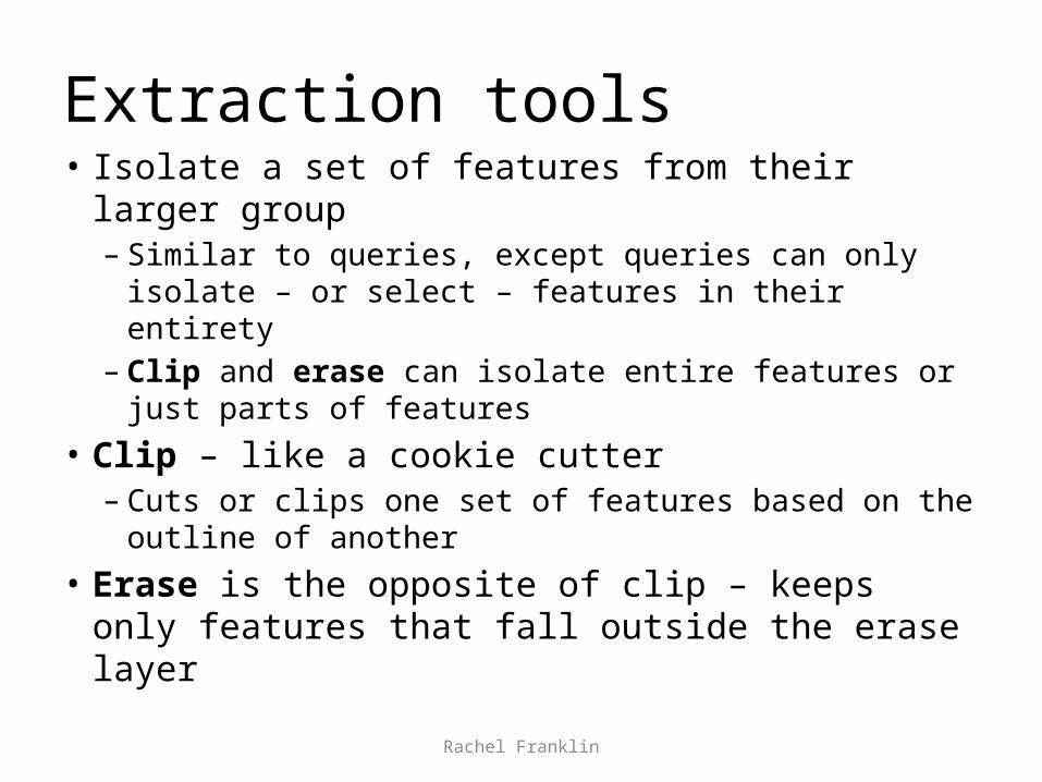
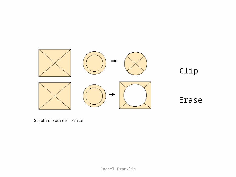
Extraction tools• Isolate a set of features from their larger

group– Similar to queries, except queries can only

isolate – or select – features in their entirety– Clip and erase can isolate entire features or

just parts of features

• Clip – like a cookie cutter– Cuts or clips one set of features based on the

outline of another

• Erase is the opposite of clip – keeps only features that fall outside the erase layer

Rachel Franklin

Clip

Erase

Graphic source: Price

Rachel Franklin

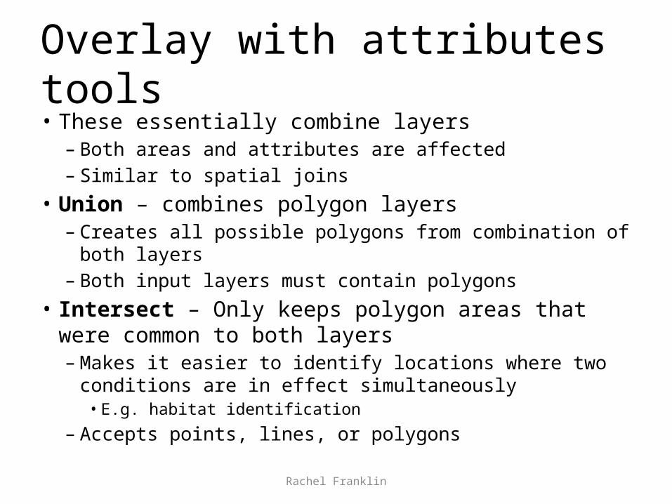
Overlay with attributes tools• These essentially combine layers

– Both areas and attributes are affected– Similar to spatial joins

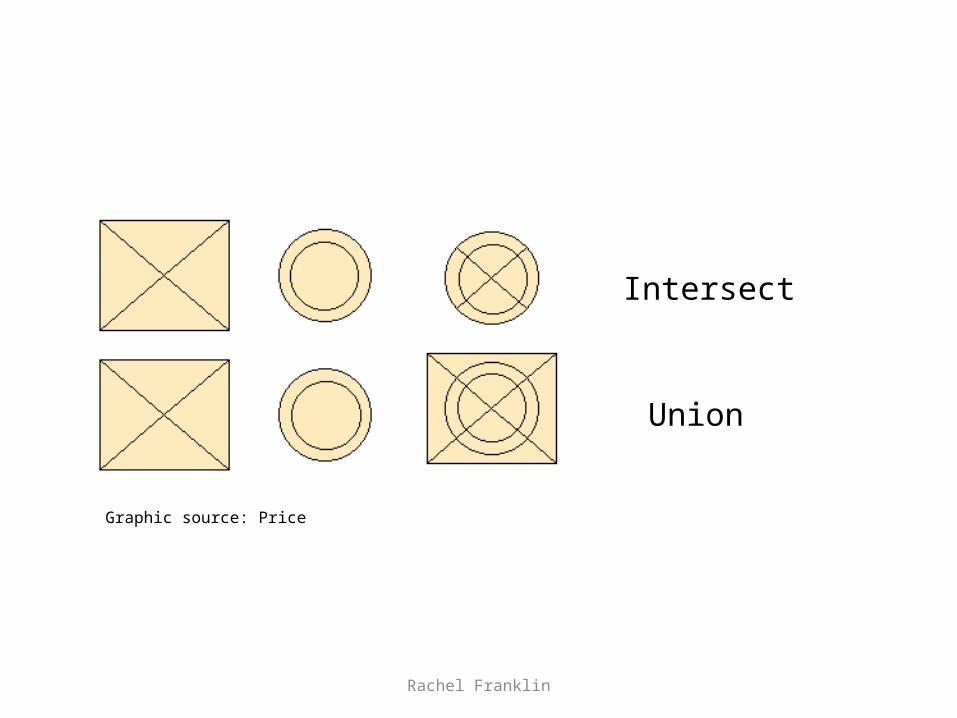
• Union – combines polygon layers– Creates all possible polygons from combination of both

layers– Both input layers must contain polygons

• Intersect – Only keeps polygon areas that were common to both layers– Makes it easier to identify locations where two

conditions are in effect simultaneously• E.g. habitat identification

– Accepts points, lines, or polygons

Rachel Franklin

Intersect

Union

Graphic source: Price

Rachel Franklin

Other common tools (found in ArcToolbox)

• Dissolve – groups features together, based on a common attribute

• Buffer – identifies areas that fall within a certain distance of a set of features

• Append and Merge – combine features from two or more layers– Layers must be the same feature type– And have the same coordinate system

Rachel Franklin

Geoprocessing with ArcGIS• Geoprocessing tools are accessible

via:– ArcToolbox–Menus and tool bars– Command line

• ModelBuilder and scripts• Pay special attention to:– Coordinate systems and projections– Areas and lengths


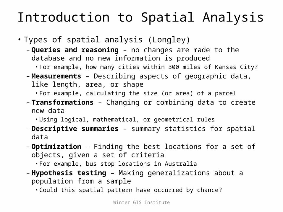
Introduction to Spatial Analysis• Types of spatial analysis (Longley)

– Queries and reasoning – no changes are made to the database and no new information is produced• For example, how many cities within 300 miles of Kansas City?

– Measurements – Describing aspects of geographic data, like length, area, or shape• For example, calculating the size (or area) of a parcel

– Transformations – Changing or combining data to create new data• Using logical, mathematical, or geometrical rules

– Descriptive summaries – summary statistics for spatial data

– Optimization – Finding the best locations for a set of objects, given a set of criteria• For example, bus stop locations in Australia

– Hypothesis testing – Making generalizations about a population from a sample• Could this spatial pattern have occurred by chance?


Queries and Reasoning• We can query our spatial data lots of

ways:– Through perusing the “catalog” or file view–Map view– Table view– Histogram or scatterplot view– Database queries, using SQL

• Remember, “computers are generally uncomfortable with vagueness.” (Longley)


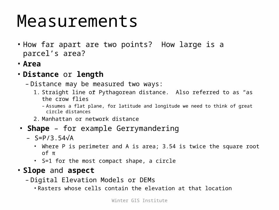
Measurements• How far apart are two points? How large is a parcel’s area?• Area• Distance or length

– Distance may be measured two ways:1. Straight line or Pythagorean distance. Also referred to as “as the

crow flies”– Assumes a flat plane, for latitude and longitude we need to think of great circle

distances

2. Manhattan or network distance

• Shape – for example Gerrymandering– S=P/3.54√A

• Where P is perimeter and A is area; 3.54 is twice the square root of π• S=1 for the most compact shape, a circle

• Slope and aspect– Digital Elevation Models or DEMs

• Rasters whose cells contain the elevation at that location


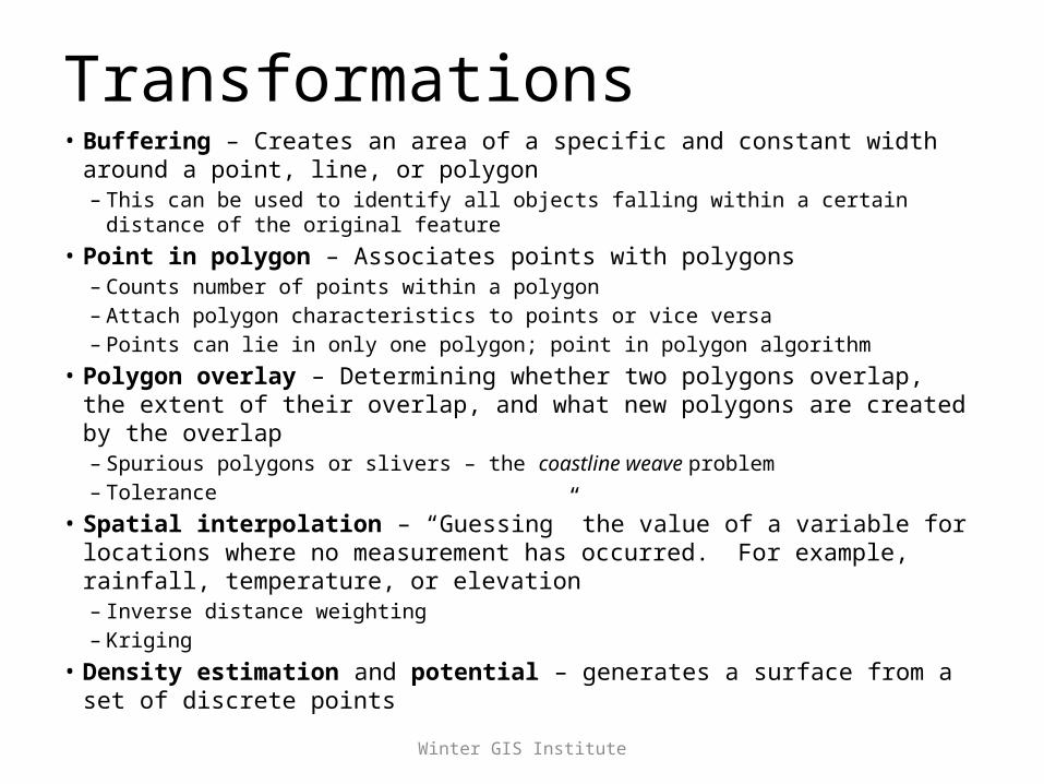
Transformations• Buffering – Creates an area of a specific and constant width around a

point, line, or polygon– This can be used to identify all objects falling within a certain distance of the

original feature

• Point in polygon – Associates points with polygons– Counts number of points within a polygon– Attach polygon characteristics to points or vice versa– Points can lie in only one polygon; point in polygon algorithm

• Polygon overlay – Determining whether two polygons overlap, the extent of their overlap, and what new polygons are created by the overlap– Spurious polygons or slivers – the coastline weave problem– Tolerance

• Spatial interpolation – “Guessing” the value of a variable for locations where no measurement has occurred. For example, rainfall, temperature, or elevation– Inverse distance weighting– Kriging

• Density estimation and potential – generates a surface from a set of discrete points


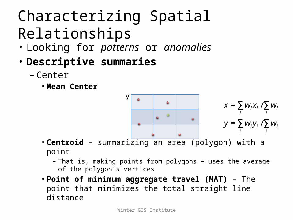
Characterizing Spatial Relationships• Looking for patterns or anomalies• Descriptive summaries– Center

• Mean Center

• Centroid – summarizing an area (polygon) with a point– That is, making points from polygons – uses the average of

the polygon’s vertices

• Point of minimum aggregate travel (MAT) – The point that minimizes the total straight line distance

€

x =iΣwix i /

iΣwi

y =iΣwiy i /

iΣwi

y


– Dispersion• Mean distance from the centroid

– Spatial Dependence• We can think of global and local measures of spatial

dependence• The scale we use will determine, in large part,

whether we find spatial dependence across a set of objects

– Fragmentation – how broken up is the landscape into difference pieces?• Are these pieces large or small? Compact or spread

out?• One measure is simply the number of patches that

exist• Or we can use the shape measure discussed a few

minutes ago: S=P/3.54√A


Optimization• Best location for a set of points– “p-median problem” – seeking the best

location for a set of p facilities, such that distance from each point to the closest facility is minimized• School location, e.g.

– “Coverage problem” – seeking to minimize the furthest distance traveled• Fire station location, e.g.

– “Location-Allocation” – We’re not only trying to locate facilities, but also allocate demand for each facility


Optimization, continued• Routing on a network

– “Shortest path” – The best path through a network that minimizes distance or travel time• Google Maps direction, e.g.

– “Traveling Salesman Problem” (TSP) – Seeks the best ordering of a set of stops to minimize total distance traveled• My milkman, e.g.• If there are n places to be visited including home base,

then there are (n-1)! possible tours to choose from– Or, really, (n-1)!/2, since it doesn’t matter if a given tour is

done forwards or backwards.

• Large n problem and the use of heuristics


Optimization, continued• Optimum paths - best paths in continuous

space– Locating highways or power lines, for example– Routing airplane flights

• These are often solved using a raster, where each cell contains a friction value – cost or time associated with crossing the cell– GIS then finds the least-cost path

• We can differentiate between optimal locations with a network or just in continuous space


Quantifying Spatial Relationships

• Point patterns– Is the distribution of points random?

Uniform? Can we identify clusters?

• Measures of spatial association– Global – Do we see positive or negative

autocorrelation across our study area• Very dependent on scale

– Local – Are values correlated with local neighbors?• House values• Crime


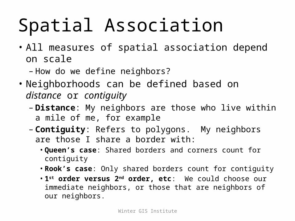
Spatial Association• All measures of spatial association depend on

scale– How do we define neighbors?

• Neighborhoods can be defined based on distance or contiguity– Distance: My neighbors are those who live within a

mile of me, for example– Contiguity: Refers to polygons. My neighbors are

those I share a border with:• Queen’s case: Shared borders and corners count for

contiguity• Rook’s case: Only shared borders count for contiguity• 1st order versus 2nd order, etc: We could choose our

immediate neighbors, or those that are neighbors of our neighbors.


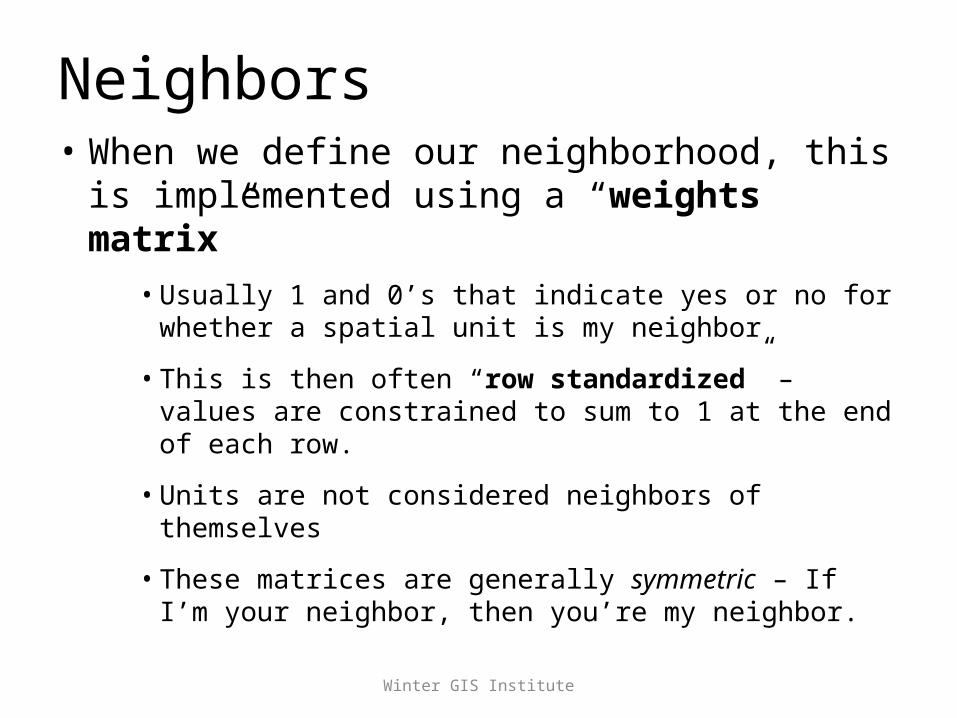
Neighbors• When we define our neighborhood, this

is implemented using a “weights matrix”

• Usually 1 and 0’s that indicate yes or no for whether a spatial unit is my neighbor

• This is then often “row standardized” – values are constrained to sum to 1 at the end of each row.

• Units are not considered neighbors of themselves

• These matrices are generally symmetric – If I’m your neighbor, then you’re my neighbor.


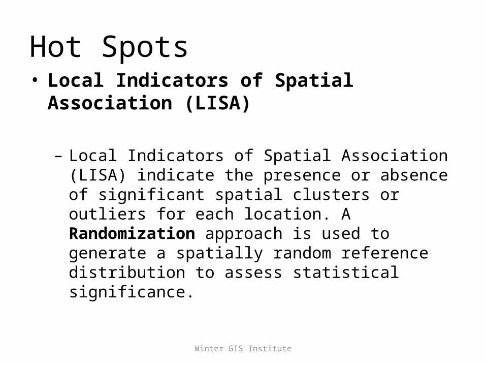
Hot Spots• Local Indicators of Spatial Association

(LISA)

– Local Indicators of Spatial Association (LISA) indicate the presence or absence of significant spatial clusters or outliers for each location. A Randomization approach is used to generate a spatially random reference distribution to assess statistical significance.


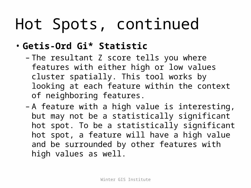
Hot Spots, continued• Getis-Ord Gi* Statistic– The resultant Z score tells you where

features with either high or low values cluster spatially. This tool works by looking at each feature within the context of neighboring features.

– A feature with a high value is interesting, but may not be a statistically significant hot spot. To be a statistically significant hot spot, a feature will have a high value and be surrounded by other features with high values as well.


Getting Data into a GIS

• A few options:– Best case scenario: data are already in

shapefile format, or similar• Or you join e.g. excel data to shapefile data

– You collect or create your data yourself– ArcGIS converts X,Y (lat, long)

coordinates into point data– Or, very commonly, we geocode


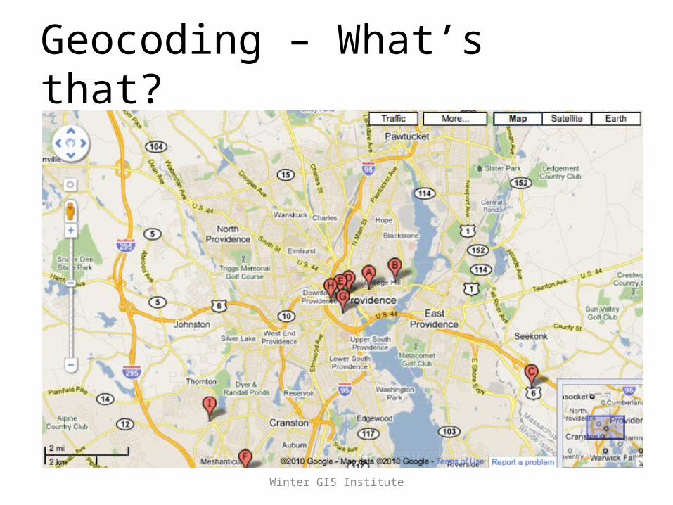
Geocoding – What’s that?

• Along with mapping, geocoding is one of the most commonly-used GIS applications

• When we geocode, we attach location information to tabular geographic information– Addresses of all grocery stores in Providence– Locations of all capital cities in the world

• We can think of a location-specificity continuum from general (e.g. cities) to specific (e.g. exact addresses)


Geocoding – What’s that?


• The more specific we are in terms of location, the more geographic information we need– Also, depending on use of geocoded

information, exact location may be very important – for example, 911 calls

– Locating cities requires a reference file with city locations

– Location addresses in Providence requires street name and street number, at a minimum

• Locations can be attached to polygons or points, but the most challenging is attaching to addresses, or lines


What’s it used for?

• Emergency services• GPS• Driving directions• Google maps• Crime analysis• Marketing


How does it work?

• Tabular data are compared to a spatial Reference layer– This is what ArcMap uses to match addresses

• This happens in a few steps– To work best, addresses need to be recognizable to the

computer, or standardized– Then standardized addresses in our table of locations (say, J.

Crew stores) are compared to our reference layer

• To understand this, think about the standard components of a street address– Prefix direction– Street name– Street type– Number– Suffix direction


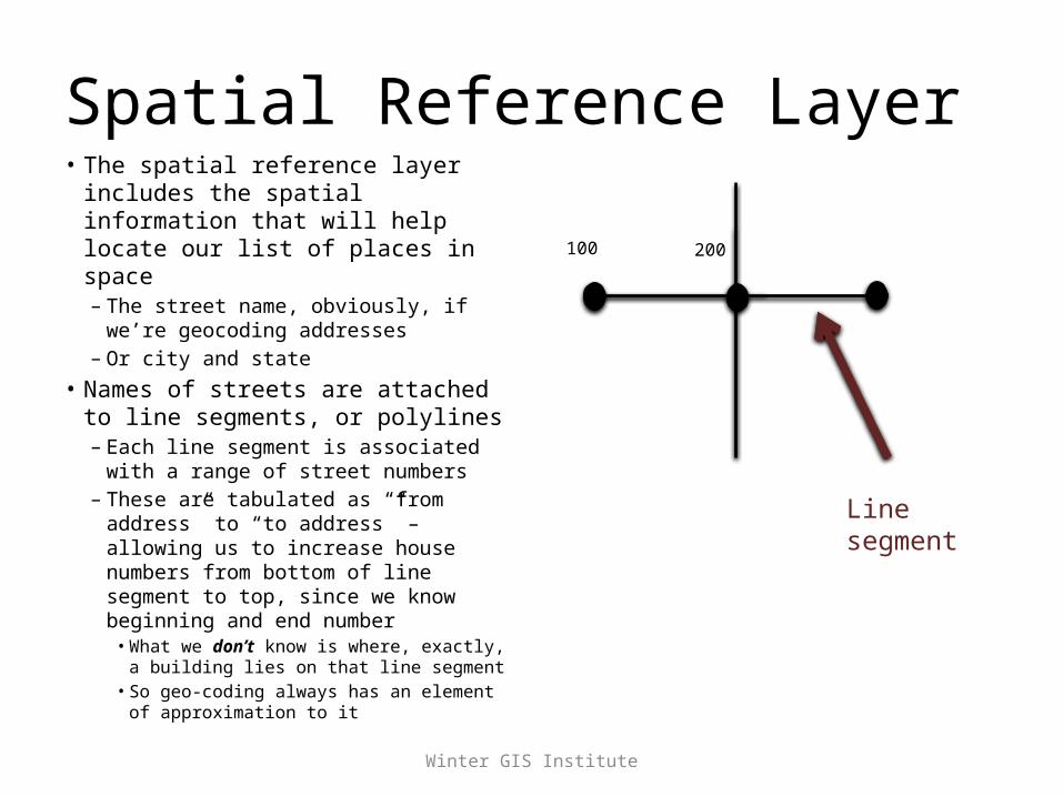
Spatial Reference Layer• The spatial reference layer

includes the spatial information that will help locate our list of places in space– The street name, obviously, if

we’re geocoding addresses– Or city and state

• Names of streets are attached to line segments, or polylines– Each line segment is associated

with a range of street numbers– These are tabulated as “from

address” to “to address” – allowing us to increase house numbers from bottom of line segment to top, since we know beginning and end number• What we don’t know is where,

exactly, a building lies on that line segment

• So geo-coding always has an element of approximation to it

Line segment

100 200


Address Geocoding• One range method: A single address range for

each chunk of street• Two range method: An address range for each side

of the street– Obviously more desirable, but not always possible since

this information needs to be coded into the reference layer

– ArcMap allows us to include an “offset” in this case

• In both cases, addresses are assigned to a place on the line in proportion to the starting and ending address on the line itself.– So if the polyline starts at 100 Main St. and ends at 200

Main St., an address of 150 Main St. goes right in the middle


Types of geocoding styles• Single field – Zip code, state name, power stations

• Alphanumeric Ranges – Helps narrow the search range for address identification, since ArcMap only has to look in that quadrant

• US Cities and states – Locates cities, given city and state names• US One Address – Matches addresses to points or polygons

• US One Range – Matches addresses to one range of street values

• US Streets – Matches addresses to a range of street values for both sides of the street

• World City and country – Locates cities within countries on a world map

• Zip code – Matches zip codes to a point or polygon reference layer

• Zone option – Additional pieces of information (zip, state, city) that allow us to match over larger areas


Why it’s important to know your study location

• Quirky address styles:– Queens, NY– Washington, DC– Phoenix, AZ

• Quickly growing locations• Spelling quirks– Saint and St. / Sainte and Ste.

• Value of “Alias Tables”– Maxcy Hall v. 112 George Street


How geocoding works in ArcGIS• First, load your address table and reference layer

into ArcMap• Then we need to set up an address locator

– Done in ArcCatalog– This assembles the pieces of information we need in

order to geocode• What is our reference layer?• What are the key fields we’ll use to locate addresses?• A “snapshot” of the reference layer is taken at this time –

important to remember

• Geocoding can be done interactively or in batch mode– Usually we do a combination of both

• The output is a new shapefile or feature class

winter 2011 gis institute geocoding & spatial analysis winter gis institute

Documents

spatial data

spatial relationships

choice of spatial units

units rachel franklin

shape of spatial units

spatial sample random

opposite rachel franklin

point random spatial