winner takes all? tech clusters, population centers, and
TRANSCRIPT

Winner Takes All? Tech Clusters, Population Centers, and the Spatial Transformation of U.S. Invention Brad Chattergoon William R. Kerr
Working Paper 22-027

Working Paper 22-027
Copyright © 2021 by Brad Chattergoon and William R. Kerr.
Working papers are in draft form. This working paper is distributed for purposes of comment and discussion only. It may not be reproduced without permission of the copyright holder. Copies of working papers are available from the author.
Funding for this research was provided in part by from Harvard Business School.
Winner Takes All? Tech Clusters, Population Centers, and the Spatial Transformation of U.S. Invention
Brad Chattergoon Harvard University
William R. Kerr Harvard Business School
1
Winner Takes All? Tech Clusters, Population Centers, and
the Spatial Transformation of U.S. Invention
Authors: Brad Chattergoon1, William R. Kerr1,2*.
Affiliations:
1Harvard University, Boston MA.
2National Bureau of Economic Research, Cambridge MA.
*Correspondence to: [email protected].
Abstract: U.S. invention has become increasingly concentrated around major tech centers since
the 1970s, with implications for how much cities across the country share in concomitant local
benefits. Is invention becoming a winner-takes-all race? We explore the rising spatial
concentration of patents and identify an underlying stability in their distribution. Software
patents have exploded to account for about half of patents today, and these patents are highly
concentrated in tech centers. Tech centers also account for a growing share of non-software
patents, but the reallocation, by contrast, is entirely from the five largest population centers in
1980. Non-software patenting is stable for most cities, with anchor tenants like universities
playing important roles, suggesting the growing concentration of invention may be nearing its
end. Immigrant inventors and new businesses aided in the spatial transformation.
One Sentence Summary: The growing concentration of patenting in tech centers masks an
important stability in non-software patenting for most U.S. cities.
JEL Codes: O30, O31, O32, O33, O34, R11, R12, L86.
Keywords: invention, patents, innovation, software, artificial intelligence, clusters,
agglomeration.
Acknowledgments: We thank Bob Hunt, Adam Jaffe, Josh Lerner, Megan MacGarvie, Mike
Webb, seminar participants, and anonymous referees for helpful comments on this project. This
research was supported by Harvard Business School. Authors declare no competing interests.
Data and code are available with online supplement: https://doi.org/10.7910/DVN/GTVSIY.

2
Introduction
The spatial distribution of invention is important for science, business, and policy. Invention
builds upon itself, and knowledge spillovers are more localized than other forms of economic
interaction.1 Consequently, tight clusters of innovation form and shape the access of individuals
and institutions to important resources necessary for this work.2 The depths of these local
technology pools influence the likelihood of achieving breakthrough inventions that draw
frontier industries to a region and the capacity of regions to recombine prior work into novel
contributions.3 The distributional implications of the spatial location of invention are significant
and long-lasting, with one study showing children raised in areas lacking invention are less likely
to become future inventors (Bell et al., 2019).
U.S. patenting has become much more spatially concentrated around tech clusters like San
Francisco and Boston compared to the 1970s, making these places more productive for
researchers in terms of their patenting propensity, important for business organization, and
central to high-tech startups.4 Astoundingly, five of the six most valuable public companies in
the world in 2020 were tech companies headquartered in San Francisco or Seattle. In response,
local policy initiatives to boost innovation abound (Chatterji et al., 2014), and 238 U.S. cities bid
for Amazon’s HQ2. Is invention becoming a winner-takes-all race?
While the growing prominence of tech clusters is important, we show in this note that it is mostly
due to two forces: 1) the rise of software patents, which are very concentrated in tech centers,
and 2) the reallocation of non-software patents to tech centers from a few big population centers.
These trends mask an important stability in the spatial distribution of non-software patents. We
trace part of this stability to dispersed anchor tenants like universities.
Our work is closely linked to Bettencourt et al. (2007) and Balland et al. (2020). Bettencourt et
al. (2007) show that patenting activity became increasingly concentrated in U.S. urban areas in
the latter decades of the 20th century and that patenting scales at a super-linear rate to city
population; Verspagen and Schoenmakers (2004) show similar spatial concentration in
multinational patenting in Europe. More recently, Balland et al. (2020) quantify that patenting
and related forms of innovation have become increasingly concentrated in larger cities.5 This
increase is linked to the capacity of big cities to conduct more complex processes; the spatial
concentration of invention has been growing since the 1850s.
We contribute to this literature in several ways. Most studies focus on quantifying the macro
relationship of patenting to city size, using data spanning small cities like Casper, WY, and Enid,
OK to the giants of New York and Los Angeles. Case studies also contemplate competition
among tech clusters, such as Saxenian’s (1996) account of the migration of semiconductors from
Boston to San Francisco. Our contribution is to quantify how much of the rise of tech centers like
Boston, Seattle, and San Francisco since the 1970s is due to a shift of patenting from the biggest
population centers in 1980 like NYC and LA. The magnitudes are large: the 13.6% reduction
from the 1970s to 2015-2019 in the patent share accounted for by the five largest population
1 Audretsch and Feldman, 1996; Ganguli et al., 2020; Jaffe et al., 1993; Rosenthal and Strange, 2020. 2 Breschi and Lissoni, 2001; Buzard et al., 2017, 2020; Kerr and Kominers, 2015; Stuart and Sorenson, 2003. 3 Bloom et al., 2021; Duranton, 2007; Duranton and Puga, 2001; Fleming and Sorenson, 2001; Jacobs, 1970; Kerr, 2010; Lin,
2011; Youn et al., 2015. 4 Alcacer and Delgado, 2016; Guzman, 2020; Guzman and Stern, 2020; Moretti, 2019; Verspagen and Schoenmakers, 2004. 5 In a model of the form y ≈ population^β, the authors estimate β equals 1.54 for published papers, 1.26 for patents, 1.11 for
GDP, and 1.04 for employment. Related, they also note a scaling of 1.57 for patents in ‘computer hardware and software’.

3
centers in 1980 is comparable to the combined patenting of the 238 MSAs with the least
patenting in 2015-2019.
We also provide new evidence linking this increasing spatial concentration to software/digital
inventions, including artificial intelligence. We draw upon algorithms by Bessen and Hunt
(2007) and Graham and Vishnubhakat (2013), as well as our own extension of these using
machine learning techniques. We measure an enormous increase in the share of patenting that is
software related, to account for almost half of patenting today. This type of invention is
conducive to spatial concentration and responsible for much of the overall rise in the
concentration of inventions. In non-software domains, the distribution of patenting is more
stable, although the shift of activity away from large population centers is still evident.6
These two trends—the reallocation of patents from a few large population centers to tech clusters
and the explosion of software patents—are nuanced and masked in aggregate assessments. The
purpose of this research note is to quantify them and raise their profile. We close by exploring
their link to factors important for innovation (e.g., universities, immigration). These preliminary
explorations are atheoretical and not conclusive, but they hopefully spark interest in follow-on
assessments.
Patent Data
We study micro-records for all utility patents granted by the United States Patent and Trademark
Office (USPTO) from January 1976 to December 2020 (Hall et al., 2001; Li et al., 2014). We
consider patents with at least one inventor in the United States and locate the work to the modal
U.S. city of inventors listed on the patent. We date patents by their application year and consider
applications made during 1975 to 2019. Our Online Supplemental Materials describe data
preparation in detail.
Defining a tech cluster requires consideration of complementary inputs to patenting like venture
capital investment.7 We follow Kerr and Robert-Nicoud (2020) and Rosenthal and Strange
(2020) by using two criteria that reflect the scale and density of local tech activity: 1) the city
ranks among the top 15 cities for patents and venture capital investment (the scale of activity)
and 2) the city holds shares for patents, venture capital, employment in R&D-intensive sectors,
and employment in digital-connected occupations that exceed its population share (the density of
activity).
Six metropolitan statistical areas (MSAs8) satisfy these scale and density criteria: San Francisco,
Boston, Seattle, San Diego, Denver, and Austin. New York and Los Angeles are ambiguous, as
the cities hold large scale but fall short on several density requirements. If we relax some
requirements, three other candidates are Raleigh-Durham, Minneapolis-St. Paul, and Washington
DC, and our Online Supplement Materials discuss robustness of the patterns documented to tech
cluster definitions.
6 As we describe further below, the line between software patents and other digitally connected inventions is blurry. The spatial
transformation we depict in this note is robust under available definitions, including one for artificial intelligence, but we do not
claim that the clustering pattern would be necessarily absent in neighboring domains. 7 Samila and Sorenson, 2011; Sorenson and Stuart, 2001. 8 Throughout, we use consolidated MSAs such that San Francisco includes San Jose, Oakland, and so on.

4
In 1980, the ten most populated MSAs were New York City, Los Angeles, Chicago,
Philadelphia, Detroit, San Francisco, Washington DC, Dallas-Ft. Worth, Houston, and Boston.
San Francisco (#6) and Boston (#10) are two of the identified tech clusters, and the next largest
is San Diego at #17 in terms of the 1980 population ranking. Our analysis focuses on the
reallocation of patenting from the five largest MSAs in 1980 in terms of population that rank
ahead of San Francisco to tech centers.
We identify software patents using algorithms based upon key words in the patent.9 We build our
main results on the algorithm developed by Bessen and Hunt (2007), as it has been commonly
used, and we later discuss alternatives.
Bessen and Hunt (2007) state: “Our concept of software patent involves a logic algorithm for
processing data that is implemented via stored instructions; that is, the logic is not ‘hard-wired.’
These instructions could reside on a disk or other storage medium or they could be stored in
‘firmware,’ that is, a read-only memory, as is typical of embedded software. But we want to
exclude inventions that do not use software as part of the invention. For example, some patents
reference off-the-shelf software used to determine key parameters of the invention; such uses do
not make the patent a software patent.”
The Bessen-Hunt algorithm requires that a utility patent description includes either the string
“software” or the strings “computer” and “program”, but it must not contain “antigen” or
“antigenic” or “chromatography”. The patent title must also not contain “chip” or
“semiconductor” or “bus” or “circuit” or “circuitry”. The patent titles and grant year of three
examples: Apparatus for identifying the type of devices coupled to a data processing system
controller (4025906, 1977); Remotely initiated telemetry calling system (5327488, 1992); and
Intelligent power cycling of a wireless modem (7308611, 2007).
Software patents have exploded as a share of patenting. During 1975-1979, 2.5% of patents are
software related, and this share is 49.9% since 2015. This tremendous growth is due to
technological changes making software widespread and legal changes allowing more intellectual
property protection.10
The Spatial Transformation of U.S. Patenting
Figure 1 shows annual rates of U.S. patenting for tech clusters and large population centers.
Beyond these two groups, we aggregate the remaining 270 MSAs and prepare a fourth group for
rural areas. The thatched portion of each series is software-related, and the solid portion is non-
software-related. Patents are dated by their application years, and the final period of 2015-2019
is not shown due to incomplete series with respect to patent counts given future grants will
occur. The share-based metrics that we focus on for most of this paper are less sensitive to this
incomplete process.
The rise of the six tech centers is very stark, and Figure 2 presents these data in terms of shares.
The six tech centers account for 11.3% of patents from 1975-1979, but surge to 34.2% for 2015-
2019. San Francisco’s growth is from 4.6% to 18.4%. While other groups decline in share, the
magnitudes and economic importance are different. The five largest population centers show the
9 Bessen and Hunt, 2007; Graham and Vishnubhakat, 2013; Hall and MacGarvie, 2010; Layne-Farrar, 2005; Webb, 2019; Webb
et al., 2018. 10 Graham and Vishnubhakat, 2013; Hunt, 2010; Lerner and Seru, 2017.

5
largest drop, from 32.2% to 18.6%. By contrast, the aggregate decline for the other 270 cities,
from 45.5% to 41.0%, is much less. Non-urban areas also decline from 11.0% to 6.1%.
This reallocation is remarkable and has not been documented in prior work. Indeed, because the
reallocation is among big cities, this movement of well more than 10% of patents is almost
completely orthogonal to the standard elasticity measured across the full city size distribution. In
a model of the form patents ≈ population^β, we estimate β=1.313 (0.037) for 1975-1979 and
β=1.397 (0.047) for 2015-2019, like prior work. Yet, if we take the patenting that occurs in tech
centers and the large population centers for 2015-2019 and re-apportion according to the relative
patent shares that were present in 1975-1979, our estimate remains almost identical at β=1.397
(0.042). In other words, the β coefficient is a big vs small city comparison and less sensitive to
shifts among bigger cities.11
By contrast, an Ellison-Glaeser (EG) metric (Ellison and Glaeser, 1997) calculates the sum of
squared deviations between the patenting shares of MSAs compared to their population shares
(with a normalization factor). The index is defined as:
𝐸𝐺 =∑ (𝑠𝑖 − 𝑝𝑖)
2𝑖
1 − ∑ 𝑝𝑖2
𝑖
where 𝑠𝑖 is the share of patenting in city i and 𝑝𝑖 is the population share. The EG index is well
suited for capturing reallocation of activity at the top end of the city size distribution. The EG
index has a value of zero if innovation is spread out the same as population; positive values
indicate concentration that differs from what one would expect based upon population.
An EG index shows a much stronger response. From a starting value of 0.003 in 1975-1979, the
EG increases ten-fold to 0.033 in 2015-2019. This increase is substantial, and if we instead re-
re-apportion recent patenting within tech clusters and large population centers according to their
relative rates in 1975-1979, our EG index only grows to 0.011. Thus, more than 70% of the rise
in the EG index is due to movements among these larger cities.
Software vs Non-Software Patenting
Figures 1 and 2 suggest that software patenting is important for our understanding of spatial
clustering and tech clusters. Software patents are a significant share of invention in all cities, but
they account for well more than half of patents in tech clusters. Panel B in Figure 2 shows that
the tech centers account for 45.4% of software patents after 2015, more than double their starting
share of 20.2%. San Francisco again features prominently with 25.8% of software patents filed
after 2015. This reallocation pulled from all regions.
Panel B of Figure 2 shows that tech clusters are also important for non-software patents (solid
lines), growing from 11.0% to 23.1% across the period. San Francisco is 11.1%. However, the
share for the 270 MSAs grows slightly from 45.5% to 48.1%. The shift is instead from the five
largest cities in 1980, which fall from 32.3% to 20.0%. These cities have remained mostly
prosperous and often hold leading positions in important sectors (e.g., media in Los Angeles,
finance in New York). But, while patents continue to increase in a super-linear relationship to
city population, invention has become less coupled to the largest cities.12
11 We exclude rural areas from this exercise and the upcoming Ellison-Glaeser calculations. 12 Carlino et al., 2007; Fritsch and Wyrwich, 2020; Lerner et al., 2020; Moretti, 2012.

6
We next separate industrial and university assignees to study agglomeration behavior. Industrial
firms have discretion over locations, such as the choice by IBM of how much of its R&D work
to conduct in its Yorktown Heights and Albany, NY, labs versus those in Cambridge, MA and
San Jose, CA. The creative destruction process also pits new entrants in tech centers against
spatially distant incumbents. By contrast, universities are local anchor tenants across the country
and mostly constrained from agglomerating.13 Research universities also rarely go out of
business.
Panel A of Figure 3 displays the EG metric for software and non-software patenting by industrial
assignees. Software patenting is more concentrated than non-software patenting, and it has
become extremely agglomerated among industrial assignees. As industrial firms account for
most patents (85.7% after 201514), their concentration principally shapes the overall
concentration of US patenting.
Panel B of Figure 3 provides a stark contrast with university patenting. While software
represents 31.5% of university patents after 2015, their spatial concentration has declined.
Concentration levels among non-software patents have also declined.
This recent role of universities in promoting the geographic stability of invention stands in
contrast to how universities contributed disproportionately in the 1970s and 1980s for the
emergence of software patents in tech centers, especially Boston and San Francisco. After this
concentrated start, however, university contributions have been more widespread. The compound
annual growth rate of university patenting from 1975 to 2015 is highest in the Other 270 Cities.
The Spread of Software Patents
In 2011, prominent venture investor Marc Andreessen famously proclaimed “software is eating
the world” (Andreessen, 2011). Indeed, Figure 4 shows that software patenting has expanded
beyond its traditional NBER technology categories of computers/communications and
electrical/electronics. For example, software patents are 15.8% of patents in chemicals and
drugs/medicines. In total for 2012, software patents represent more than a quarter of patents in
24.6% of the 410 United States Patent Classes (USPCs) that are continually present from 1975 to
2012, and more than two-thirds of classes have a greater than 5% software share by 2012.
We can decompose software’s growth using the USPC patent class system (which ends in 2012)
using the identity:
Δ𝑆𝑊𝑡 = ∑𝑐𝑖,𝑡−1Δ𝑆𝑊𝑖,𝑡 + ∑(𝑆𝑊𝑖,𝑡−1 − 𝑆𝑊𝑡−1)Δ𝑐𝑖,𝑡 + ∑Δ𝑐𝑖,𝑡Δ𝑆𝑊𝑖,𝑡
where Δ𝑆𝑊𝑡 is the change in the share of software patents between 2012 (t) and 1976 (t-1) and
𝑐𝑖,𝑡 is USPC class i’s share of patents in year t. The first term captures the within-class effect
(i.e., software becoming more prevalent as technology classes looked in 1976), the second
captures a between-class effect (i.e., classes that were software intensive in 1976 growing more
quickly), and the third term represents a cross component (i.e., classes that are becoming more
software intensive also growing more quickly).
13 Agrawal and Cockburn, 2003; Agrawal et al., 2014; Berkes and Nencka, 2019; Feldman, 2003; Hausman, 2012; Kantor and
Whalley, 2014. 14 During 1975-1979, approximately 70.2% of patents were made by industrial assignees, 1.1% by universities, 2.8% by
government, and 26.0% unassigned. For 2015-2019, these shares were 85.7%, 4.2%, 0.7%, and 9.5%, respectively. Shares can
total to more than 100% due to joint assignment of patents across institutions.

7
We calculate that 38.3% of the software patenting growth is from an increased software share
holding the 1976 distribution of patent classes constant (the within term), 36.9% from an
increase in the class shares holding constant the 1976 software intensity (the between term), and
24.7% from faster growth of classes also correlating with faster software penetration (the cross
term). These elements are visible in Figure 4 as well.
Extensions
We discuss here supporting evidence contained in the Online Supplemental Materials.
We defined tech clusters with attention to non-patenting factors (e.g., venture investment). An
alternative approach isolates absolute changes in realized patenting growth, which proves
informative.15 The four MSAs that attracted the biggest absolute change in patent counts from
1975 to 2020 are four of our tech clusters (in order): San Francisco, Seattle, Boston, and San
Diego. The next three cities in terms of the biggest absolute change in patent counts over the
period are Los Angeles, New York City, and Detroit, three of our five large 1980 population
centers. Thus, these cities still attracted more patents, as hinted at in Figure 1, but they lost
substantial relative grounds. Indeed, we can replicate our findings with just a focus on the four
tech clusters identified with this approach.
Additionally, there is a substantial stagnation and decline in the economic might of the Rust Belt
during this period. While the major Rust Belt cities (such as Buffalo, Cleveland, and Pittsburgh)
also lose a substantial share of patenting since the 1970s, this process is distinct. Among our
large 1980 population centers, Detroit and, to a lesser extent, Chicago, feature among the Rust
Belt, but they play a relatively small role in the trends we focus on.
Turning to software definition, a first question focuses on the quality of software patents.
Perhaps the explosion in patents in tech centers has been associated with deteriorations in their
quality. Using techniques like forward citations16, we do not observe any declines in patent
quality (software and non-software) for tech centers compared to other locations.
The Bessen and Hunt (BH) technique uses keywords, and a prominent technique by Graham and
Vishnubhakat (GV) defines software via patent classes. To evaluate the performance of these
approaches, we randomly sampled 1600 patents from NBER Category 2 stratified across eight
periods from 1976-79 to 2010-14. Within each period, we sampled 100 BH, 50 GV, and 50 other
patents. One patent was sampled twice, and several could not be reliably assigned, resulting in a
final sample of 1559 patents. We manually defined 788 (50.5%) of these as software patents.
Both techniques performed reasonably well and had understandable challenges. BH identified
91% of the patents that we classified as software (recall), but only 79% of BH identified patents
were ones we identified as software (precision). The parsimonious set of keywords in the BH
algorithm performs well in identifying likely software patents, and the algorithm’s weakness are
the false positives that evade the few negatively selected terms.
The GV algorithm identified 98% of the patents that we classified as software (recall), but only
68% of GV patents identified as software were manually classified as software (precision). The
15 We thank a referee for this suggestion. In the Online Supplemental Materials, we also discuss the small scope for expanding
out the tech cluster definition to include more cities like Raleigh-Durham and Minneapolis-St. Paul. 16 Harhoff et al., 1999; Hall et al., 2005.

8
patent class approach achieves a lot by identifying the classes with the most software patents,
although 98% will overstate performance if extending sample beyond NBER Category 2. GV’s
straightforward challenge is that these classes are not exclusive to software patents.
The Online Supplemental Materials show that performance of BH and GV algorithms is best
after 1995, increasing on both precision and recall from the 1970s until that point.
Using these 1559 hand-coded patents, we developed a third approach by training a machine
learning algorithm. Conceptually, this is an extension of both techniques, giving up the
transparency of BH’s keywords for a computational approach that particularly bolsters negative
selection. The training on many patents in GV classes also benefits from the technology
perspectives developed during the examination process. The algorithm is stingier in assignment
(88% recall) but has fewer false positives (85% precision).
Figure 5 shows our key findings with the three techniques. We further incorporate a definition of
AI-related patents developed by Giczy et al. (2021). The spatial reallocation of patents that this
paper emphasizes are robust across these definitions. There is important scope for further honing
patent technology divisions with computation techniques, with this robustness check perhaps
being a seed.
Future Research
This note has documented a remarkable spatial transformation of patenting due to 1) the rise of
software patents, which are very concentrated in tech centers, and 2) the reallocation of non-
software patents to tech centers from a few big population centers.
Future research should explore why software patenting rose so much in its spatial concentration.
Its higher initial concentration than patenting in traditional technologies (e.g., chemicals,
agriculture) is not too surprising, but the subsequent growth in agglomeration deserves attention.
Candidate ideas include growing technology complexity (Sorenson et al., 2006; Balland et al.,
2020), greater need to participate in tacit knowledge about technology and market trends to be
competitive, greater role of venture investment in new software startups, and greater desire for
top talent in these fields to be in certain cities.
How this concentration happened is also interesting. In the Online Supplemental Materials, we
provide preliminary evidence that software patenting growth in tech centers is facilitated through
new businesses coming to the forefront, such as Apple and Microsoft, and less due to shifts in
locations of incumbents, such as IBM. We also quantify how the increased US reliance on
immigrant inventors17 aided the speed of the spatial transition. These two early cuts suggest that
the dynamism of the U.S. innovation system, in terms of new firm formation and access to global
talent, shaped the spatial transformation.
Hidden behind these trends is an important stability in the spatial distribution of non-software
patents. Indeed, to some degree, the spatial transformation of patenting may be ending, except
for a mechanical effect, should software grow as a share of patenting. Figure 1’s trends taper off
over the last two decades, and the underlying patenting shares of cities are becoming calcified.18
17 Bernstein et al., 2019; Hunt and Gauthier-Loiselle, 2010; Kerr and Lincoln, 2010; Peri et al., 2015; Stephan and Levin, 2001. 18 To illustrate, a vector of non-software patenting shares for cities in 2015-2019 displays a 0.970 correlation to a similar vector
for 1995-1999, whereas the correlation between the vectors for 1995-1999 and 1975-1979 is lower at 0.877.

9
Despite software’s growth across technologies, non-traditional sectors have yet to experience a
substantial agglomeration around tech clusters like what transpired in
computers/communications and electrical/electronics.
The pandemic raises many ongoing debates about future spatial concentration and tech clusters.
Yet, even without the pandemic’s emergence, this paper shows that the underlying stability of
non-software patenting is likely to continue and ensure a broader spatial distribution of
innovation. Regional advantages for being a premier location for invention will likely remain the
subject of intense local competition19, but these spatial dynamics suggest the remarkable recent
increases in the concentration of local invention are unlikely to segue into a winner-takes-all
race.
References:
Agrawal, A. & I. Cockburn. (2003). The anchor tenant hypothesis: exploring the role of large,
local, R&D-intensive firms in regional innovation systems. International Journal of Industrial
Organization 21(9), 1217-1253.
Agrawal, A., I. Cockburn, A. Galasso & A. Oettl. (2014). Why are some regions more innovative
than others? the role of small firms in the presence of large labs. Journal of Urban Economics
81(1), 149-165.
Alcacer, J. & M. Delgado. (2016). Spatial organization of firms and location choices through the
value chain. Management Science 62(11), 3213-3234.
Andreessen, M. (2011). Why software is eating the world. Wall Street Journal.
https://www.wsj.com/articles/SB10001424053111903480904576512250915629460
Audretsch, D.B. & M.P. Feldman. (1996). R&D spillovers and the geography of innovation and
production. American Economic Review 86(3), 630-640.
Balland, P.A., C. Jara-Figueroa, S.G. Petralia, M.P.A. Steijn, D.L. Rigby & C.A. Hidalgo. (2020).
Complex economic activities concentrate in large cities. Nature Human Behavior 4, 248-254
https://doi.org/10.1038/s41562-019-0803-3.
Bell, A., R. Chetty, X. Jaravel, N. Petkova & J. Van Reenen. (2019). Who becomes an inventor in
America? The importance of exposure to innovation. Quarterly Journal of Economics 134(2), 647-
713.
Berkes, E. & P. Nencka. (2019). ‘Novel’ ideas: the effects of Carnegie libraries on innovative
activities. Working Paper.
Bernstein, S., R. Diamond, T. McQuade & B. Pousada. (2019). The contribution of high-skilled
immigrants to innovation in the United States. Working Paper.
Bessen, J. & R.M. Hunt. (2007). An empirical look at software patents. Journal of Economics and
Management Strategy 16(1), 157-189.
19 Chatterji et al., 2014; Gruber and Johnson, 2019; Moretti, 2012; Saxenian, 1996.

10
Bettencourt, L., J. Lobo & D. Strumsky. (2007). Invention in the city: increasing returns to
patenting as a scaling function of metropolitan size. Research Policy 36, 107-120.
10.1016/j.respol.2006.09.026.
Bloom, N., T.A. Hassan, A. Kalyani, J. Lerner, and A. Tahoun. (2021). The diffusion of disruptive
technologies. NBER Working Paper 28999.
Breschi, S. & F. Lissoni. (2001). Knowledge spillovers and local innovation systems: a critical
survey. Industrial and Corporate Change 10(4), 975-1005.
Buzard, K., G. Carlino, R.M. Hunt, J. Carr & T. Smith. (2017). The agglomeration of American
R&D labs. Journal of Urban Economics 101, 14-26.
Buzard, K., G. Carlino, R.M. Hunt, J. Carr & T. Smith. (2020). Localized knowledge spillovers:
evidence from the spatial clustering of R&D labs and patent citations. Regional Science and Urban
Economics 81, 103490.
Carlino, G.A., S. Chatterjee & R.M. Hunt. (2007). Urban density and the rate of invention. Journal
of Urban Economics 61(3), 389-419.
Chatterji, A., E. Glaeser & W. Kerr. (2014). Clusters of entrepreneurship and innovation.
Innovation Policy and the Economy 14, 129-166.
Duranton, G. 2007. Urban evolutions: the fast, the slow, and the still. American Economic Review
97(1), 197-221.
Duranton, G. & D. Puga. (2001). Nursery cities: urban diversity, process innovation, and the life
cycle of products. American Economic Review 91(5), 1454-1477.
Ellison, G. & E. Glaeser. (1997). Geographic concentration in U.S. manufacturing industries: a
dartboard approach. Journal of Political Economy 105(5), 889-927.
Feldman, M. (2003). The locational dynamics of the US biotech industry: knowledge externalities
and the anchor hypothesis. Industry and Innovation 10(3), 311-329.
Fleming, L. & O. Sorenson. (2001). Technology as a complex adaptive system: evidence from
patent data. Research Policy 30(7), 1019-1039.
Fritsch, M. & M. Wyrwich. (2020). Is innovation (increasingly) concentrated in large cities? an
international comparison. Working paper.
Ganguli, I., J. Lin & N. Reynolds. (2020). The paper trail of knowledge spillovers: evidence from
patent interferences. American Economic Journal: Applied Economics 12(2), 278-302.
Giczy, A., N. Pairolero & A. Toole. (2021). Identifying artificial intelligence (AI) invention: A
novel AI patent dataset. USPTO Economic Working Paper No. 2021-2.
Graham, S. & S. Vishnubhakat. (2013). Of smart phone wars and software patents. Journal of
Economic Perspectives 27(1), 67-86.
Gruber, J. & S. Johnson. (2019). Jump-Starting America: How Breakthrough Science Can Revive
Economic Growth and the American Dream. New York: Public Affairs.
Guzman, J. (2020). Go west young firm: the value of entrepreneurial migration for startups and
their founders. Working Paper.

11
Guzman, J. & S. Stern. (2020). The state of American entrepreneurship: new estimates of the
quality and quantity of entrepreneurship for 32 US states, 1988–2014. American Economic
Journal: Economic Policy, forthcoming.
Hall, B., A. Jaffe & M. Trajtenberg. (2001). The NBER patent citation data file: lessons, insights
and methodological tools. NBER Working Paper 8498.
Hall, B.H., A. Jaffe & M. Trajtenberg. (2005). Market value and patent citations. RAND Journal
of Economics 36(1), 16-38.
Hall, B. & M. MacGarvie. (2010). The private value of software patents. Research Policy 39(7),
994-1009.
Harhoff, D., F. Narin, F.M. Scherer & K. Vopel. (1999). Citation frequency and the value of
patented inventions. Review of Economics and Statistics 81(3), 511-515.
Hausman, N. (2012). University innovation, local economic growth, and entrepreneurship. Center
for Economic Studies Paper 12-10.
Hunt, J. & M. Gauthier-Loiselle. (2010). How much does immigration boost innovation? American
Economic Journal: Macroeconomics 2(2), 31-56.
Hunt, R. (2010). Business method patents and U.S. financial services. Contemporary Economic
Policy 28, 322-352.
Jacobs, J. 1970. The Economy of Cities. New York: Vintage Books
Jaffe, A.B., M. Trajtenberg & R. Henderson. (1993). Geographic localization of knowledge
spillovers as evidenced by patent citations. Quarterly Journal of Economics 108(3), 577-598.
Kantor, S. & A. Whalley. (2014). Knowledge spillovers from research universities: evidence from
endowment value shocks. Review of Economics and Statistics 96(1), 171-188.
Kerr, W.R. (2010). Breakthrough inventions and migrating clusters of innovation. Journal of
Urban Economics 67(1), 46-60.
Kerr, W.R. & S.D. Kominers. (2015). Agglomerative forces and cluster shapes. Review of
Economics and Statistics 97(4), 877–899.
Kerr, W.R. & W. Lincoln. (2010). The supply side of innovation: H-1B visa reforms and U.S.
ethnic invention. Journal of Labor Economics 28(3), 473-508.
Kerr. W.R. & F. Robert-Nicoud. (2020). Tech clusters. Journal of Economic Perspectives 34(3),
50-76.
Layne-Farrar, A. (2005). Defining software patents: a research field guide. SSRN Electronic
Journal. DOI:10.2139/ssrn.1818025.
Lerner, J. & A. Seru. (2017). The use and misuse of patent data: issues for corporate finance and
beyond. NBER Working Paper 24053.
Lerner, J., A. Seru, N. Short & Y. Sun. (2020). Financial innovation in the 21st century: evidence
from U.S. patenting. Working Paper.
Li, G.C., R. Lai, A. D’Amour, D.M. Doolin, Y. Sun, V.I. Torvik, Z.Y. Amy, and L. Fleming.
(2014). Disambiguation and co-authorship networks of the US patent inventor database (1975–
2010). Research Policy 43(6), 941-955.
12
Lin, J. (2011). Technological adaptation, cities, and new work. Review of Economics and Statistics
93(2), 554-574.
Moretti, E. (2012). The New Geography of Jobs. New York: Houghton Mifflin Harcourt.
Moretti, E. (2019). The effect of high-tech clusters on the productivity of top inventors. NBER
Working Paper 26270.
Peri, G., K. Shih & C. Sparber. (2015). STEM workers, H-1B visas and productivity in U.S. cities.
Journal of Labor Economics 33(S1), S225-S255.
Rosenthal, S. & W. Strange. (2020). How close is close? the spatial reach of agglomeration
economies. Journal of Economic Perspectives 34(3), 27-49.
Samila, S. & O. Sorenson. (2011). Venture capital, entrepreneurship, and economic growth.
Review of Economics and Statistics 93(1), 338-349.
Saxenian, A.L. (1996). Regional Advantage: Culture and Competition in Silicon Valley and Route
128. Cambridge, MA: Harvard University Press.
Sorenson, O., J.W. Rivkin, & L. Fleming. (2006). Complexity, networks and knowledge flow.
Research Policy 35(7), 994-1017.
Sorenson, O. & T.E. Stuart. (2001). Syndication networks and the spatial distribution of venture
capital investments. American Journal of Sociology 106(6), 1546-1588.
Stephan, P. & S. Levin. (2001). Exceptional contributions to US science by the foreign-born and
foreign-educated. Population Research and Policy Review 20(1), 59-79.
Stuart, T. & O. Sorenson. (2003). The geography of opportunity: spatial heterogeneity in founding
rates and the performance of biotechnology firms. Research Policy 32(2), 229-253.
Verspagen, B. & W. Schoenmakers. (2004). The spatial dimension of patenting by multinational
firms in Europe. Journal of Economic Geography 4, 23-42.
Webb, M. (2019). The impact of artificial intelligence on the labor market. Working Paper.
Webb, M., N. Short, N. Bloom & J. Lerner. (2018). Some facts of high-tech patenting. NBER
Working Paper 24793.
Youn, H., D. Strumsky, L.M.A Bettencourt & J. Lobo. (2015). Invention as a combinatorial
process: evidence from US patents. Journal of the Royal Society Interface 12(106), 20150272.

13

14

15

16

17

Materials and Methods
1. Additional Information on Data
We utilize the patent records created and held by the United States Patent and Trademark Office (USPTO).
Our data source is the PatentsView.org web API. Established in 2012 by the Obama administration,
PatentsView provides a standardized database of patent records that “longitudinally links inventors, their
organizations, locations, and overall patenting activity.” (source: https://www.patentsview.org/web/).
PatentsView contains all patent records starting with patents granted in 1976, and our download from
spring 2021 contains records through December 31, 2020. This paper considers patent records with
application dates from the start of 1975 through the end of 2019. The use of application dates for patents
is better suited for the timing of innovation, as the USPTO’s review procedure can take multiple years and
varies across fields.
We downloaded the following fields (not all of which have employed in our study):
• Patent Data: Patent Number; Patent Date (Grant Date); Patent Abstract; Patent Kind (Patent Kind
code, e.g. B1, B2, S, P1); Patent Type (Functional category of Patent, e.g. Utility, Design, Plant);
Patent Title; Number of Claims in Patent; Application Date of Patent; List of Patent Numbers for
Cited Patents; List of Patent Numbers for Citing Patents
o United States Patent Classification Codes (USPC): USPC Mainclass ID; USPC Subclass ID;
Sequence (Order Priority of USPC code)
o NBER Category Codes: NBER Category ID; NBER Subcategory ID
o Cooperative Patent Classification (CPC) Codes: CPC Section ID; CPC Subsection ID; CPC
Group ID; CPC Subgroup ID; Sequence (Order Priority of CPC code)
• Inventor Data: Inventor ID (assigned by PatentsView); First Name; Last Name; City; State; State
FIPs; County FIPs; Country; Sequence (Order Priority of Inventor on Patent)
• Assignee Data: Assignee ID (assigned by PatentsView); Organization Name; First Name; Last
Name; City; State; State FIPs; County FIPs; Country; Assignee Type (discussed below); Sequence
(Order Priority of Assignee)
Notes about requested fields and their preparation:
• The USPC system was retired at the beginning of 2015 in favor of the CPC system, jointly
developed by the USPTO and the European Patent Office to code Utility patents. The USPC system
remains in place for other patent types, e.g. Design and Plant. For statistics in the paper, we use
the older USPC system (e.g., level of software penetration into non-traditional patent classes)
since it covered the full duration of our sample period excepting the last few years.
• We also use the NBER Category system that aggregates the USPC patent classes, as initially started
by Hall et al. (2001). To extend the NBER system to the end of our data, we developed a
probabilistic mapping of CPC codes to NBER categories and subcategories based upon the
transition period during which the USPTO assigned both CPC and USPC codes to granted patents.
• The Assignee Type refers to the organizational character of the assignee.

o PatentsView provides the following classifications for Assignee Type: US Company or
Corporation; Foreign Company or Corporation; US Individual; Foreign Individual; US
Government; Foreign Government; Country Government; and State Government (US).
We group these categories into “Industrial”, “Government”, and “Individual”.
▪ Note that an Individual assignee indicates a person has a claim to the property
rights of the patent. This is separate from the inventor designations below. Every
patent has listed inventors, but the assignment of patents to individuals is rare.
Most inventors working for a university, corporation, or government have agreed
to assign the rights of an invention over to their employer.
o We also construct a “University” classification to represent academic and research
institutions using automated and manual procedures:
▪ If an assignee’s name includes the strings “university”, “college”, “institute of
technology”, “research foundation”, “research institute”, or “polytechnic
institute”, we classify it as a “University” patent. We verified the accuracy on the
classification for the top 2000 patent assignees by number of patents.
▪ During this manual review, we also identified several academic organizations that
are best classified as a University but did not have the above the naming
conventions (e.g. Dana-Farber Cancer Institute, Inc.; Georgia Tech Research
Corporation).
▪ We remove the PatentsView-based designation (e.g. Industrial) when classifying
an assignee as a university. As such, the assignee types are mutually exclusive and
collectively exhaustive, but patents can have multiple assignees with different
assignee types.
• PatentsView provides geographic data identifying country and city, in addition to state and county
codes for US-based inventors and assignees. For most records, we map the provided county FIPs
codes into Metropolitan Statistical Areas (MSA). The county code is missing in a small share of US
cases, and, where possible, we use the city and state to repair the missing code.
o We require patents to have at least one inventor located in the United States, and we do
not further consider foreign inventors in our analysis.
o Patents can contain multiple inventors in different locations. If there is a unique most
common MSA, we use that as the spatial location of the patent. We use the highest rank
inventor’s location when a tie exists.
• To identify software patents, our main algorithm follows Bessen and Hunt (2007). Section 3 of this
Supplement discuss additional procedures for identifying software patents in detail. The Bessen
and Hunt (2007) approach that underlies most of our results:
o Patent must be a Utility Patent but not a Reissued Patent. We screen via limiting patents
to Patent Kinds “A”, “B1”, and “B2”.
o The patent description must include either the string “software” or the strings
“computer” and “program”, but must not contain “antigen” or “antigenic” or
“chromatography”.
o The patent title must not contain “chip” or “semiconductor” or “bus” or “circuit” or
“circuitry”.
• To identify inventor ethnicity, we follow a procedure that utilizes the names of inventors and
ethnic name algorithms: e.g., mapping the surnames “Patel” and “Gupta” to the Indian ethnicity
and those with “Rodriguez” and “Hernandez” to the Hispanic ethnicity. The algorithms combine
common name conventions with ethnic name databases first developed for marketing purposes.
o Ethnicity is assigned at the inventor level and then aggregated to the patent level by
averaging over inventors, thus giving equal weight to each patent in aggregate statistics.
o The procedure is laid out in detail in these papers:
▪ Kerr, W. & W. Lincoln. (2010). The Supply Side of Innovation: H-1B Visa Reforms
and U.S. Ethnic Invention. Journal of Labor Economics 28(3), 473–508.
▪ Kerr, W. (2007). The Ethnic Composition of U.S. Inventors. Harvard Business
School Working Paper 08-006.
Table S1 documents several measures for cities using data from around 2015-2018 that we employ to
define a tech cluster. (Table S1 and the next three paragraphs are taken from Kerr and Robert-Nicoud
(2020) with small modification.) The table contains the top 15 MSAs in terms of venture investment. This
table speaks best to the scale of tech activity across cities and, through a comparison to the population
share in Column 7, the implied density of tech efforts. The top 15 MSAs as ranked by venture capital
investment hold 94% of venture capital activity in Column 1 and 57% of patenting in Column 2, compared
to just 31% of population. If we instead rank on patents, Detroit, Portland, Dallas-Ft. Worth, and Houston
feature in the 15 largest centers, with Washington, Miami, Atlanta, and Raleigh-Durham dropping out.
Either way, patenting and especially venture capital investment are under-represented outside of leading
tech centers.
Columns 3 and 4 of Table S1 next provide two measures of local employment in leading industries for R&D
investment as measured by National Science Foundation (2017). We first show a restrictive definition,
where we identify college-educated workers earning more than $50,000 (short-hand labelled as “high-
skilled”) and working in a top 10 R&D-intensive sector—11.7% of such individuals work in the San
Francisco area, compared to 5.9% of them being outside metropolitan areas. The second measure
broadens to any full-time employee (no education or salary restriction) among the 20 most R&D-intensive
sectors. Column 5 similarly looks at high-skilled workers in occupations in computer- and digital-
connected work, and Column 6 expands to all full-time workers in a broader class of STEM-connected
occupations.
This table shows the potential and challenges of defining tech clusters using the scale and density of local
tech activity. Six cities appear to qualify under any aggregation scheme: San Francisco, Boston, Seattle,
San Diego, Denver, and Austin all rank among top 15 locations for venture capital and for patents (scale)
and hold shares for venture capital, patents, employment in R&D-intensive sectors, and employment in
digital-connected occupations that exceed their population shares (density). These six cities are our core
group for analysis. Washington, Minneapolis-St. Paul, and Raleigh-Durham would join the list if relaxing
the expectation that that share of venture investment exceed population share (which is hard due to the
very high concentration in San Francisco). These three borderline cases grow from 3.8% to 5.2% of US
patents during our sample period, and thus their inclusion would be consistent with our results but also
not greatly influence them.

New York and Los Angeles are more ambiguous: they hold large venture capital markets, but their patents
and employment shares in key industries and fields are somewhat less than their population shares. They
account for 7% of the patent share decline. At the other end of the city size distribution, it is hard to be a
robust-yet-small tech cluster on both venture investment and patent metrics due to the concentration of
innovation. If one only requires that a tech cluster achieve a venture capital and patent share that is 1.5x
the local population share, the one new city would be Provo, UT, with Denver dropping out.
The reallocation that we emphasize in this paper is separate from the declines in industrial activity for the
“Rust Belt” of America. As a representative calculation, the collective share of patenting in Buffalo NY,
Cincinnati OH, Cleveland OH, Columbus OH, Indianapolis IN, Milwaukee WI, Pittsburgh PA, and St. Louis
MO declined from 9.3% in 1975-1984 to 4.4% after 2015. Detroit is among the five major population
centers in 1980 but does not play a significant role its decline as its patenting share grows slightly during
the period. The dynamic is also not connected to a broad mean reversion phenomenon from 1980 stature:
exactly half of the 20 largest cities in 1980 grow their patenting share and half experience declines.
2. Supporting Data Analysis and Statistical Methods
Table S2 tabulates the data used in Figure 2 of the main text.
We use two common measures to capture the agglomeration of innovative activity as documented in our
patent dataset: the Herfindahl-Hirschman Index (HHI) and the Ellison-Glaeser (EG) Index. We apply these
two metrics at the Metropolitan Statistical Area (MSA) level.
Let si represent the share of patents in MSA i:
𝑠𝑖 =𝑁𝑢𝑚𝑏𝑒𝑟 𝑜𝑓 𝑃𝑎𝑡𝑒𝑛𝑡𝑠 𝑖𝑛 𝑀𝑆𝐴𝑖
𝑇𝑜𝑡𝑎𝑙 𝑁𝑢𝑚𝑏𝑒𝑟 𝑜𝑓 𝑃𝑎𝑡𝑒𝑛𝑡𝑠
The HHI is defined as the sum of the squared shares of patenting held by MSAs:
𝐻𝐻𝐼 = ∑ 𝑠𝑖2
𝑖
The EG (Ellison and Glaeser 1997) index incorporates more information than the HHI by including the
underlying population share of the geographic unit as a benchmark against which to compare innovation
shares. Define the MSA population share as pi.
𝑝𝑖 =𝑃𝑜𝑝𝑢𝑙𝑎𝑡𝑖𝑜𝑛 𝑜𝑓 𝑀𝑆𝐴𝑖
𝑇𝑜𝑡𝑎𝑙 𝑃𝑜𝑝𝑢𝑙𝑎𝑡𝑖𝑜𝑛
Then we define the EG index as follows:
𝐸𝐺𝐼 =∑ (𝑠𝑖 − 𝑝𝑖)2
𝑖
1 − ∑ 𝑝𝑖2
𝑖

The EG metric takes a value of zero if innovation is spread out the same as population. Positive values
indicate concentration that differs from what one would expect based upon population. This metric
captures better than an HHI metric the reallocation of patenting among large cities.
Table S3 documents the patent counts, software share, and HHI and EG concentration levels for all patents
and broken out into three major groups based upon the NBER categories: Computers and
Communications together with Electrical and Electronics, Chemical together with Drugs and Medical, and
Mechanical together with Miscellaneous/Others. This table shows the growth in software patenting in
multiple technology areas and the rising EG values for software. It is noticeable that concentration levels
are not rising substantially outside of software categories.
Figure S1 is a companion figure to Figure 4 in the main text. It shows the absolute patent counts used to
generate the patent shares made up by each combination of NBER category and software relevance. This
figure does not include the final period of 2015-2019 applications as the full level of patenting is not well
established for that period yet due to the grants still in progress; Figure 4’s composition is better assessed.
Figure S2 displays a correlation plot that models the stability of the spatial distribution of patenting across
MSAs for software and non-software patents. High correlations, indicated by dark shading, measure that
there has been very little change from one period to the other in patenting shares. This figure highlights
the significant shift through the 1990s from an earlier spatial stability to the current one. This aligns with
the significant shift in patent from the 1980 population centers into the tech clusters, with less subsequent
movement once most of the transition occurred. The spatial distribution of software shows a stronger
shift than non-software patenting.
Table S4 repeats Table S3 with breakouts by types of patent assignee: Industrial, University, Government,
or Unassigned. Industrial patents are the majority and grow to be 85.7% of patents during 2015-2019.
University patents are also a growing share, while government and unassigned patents are declining in
absolute count and share. The EG values by assignee type from this table are used in Figure 3.
Tables S5a-S5b compare metrics of patent quality for tech clusters versus elsewhere for software and
non-software patents, respectively. The first three metrics are directly from the patent data: number of
claims, number of backward citations, and number of forward citations. The fourth metric recalculates
forward citations excluding citations from the same assignee, and have also confirmed similar results
when excluding citations from the same MSA as any inventor on the focal patent. (Forward looking
measures have natural attrition in later periods as a shorter time horizon is used in their calculations.)
We also compute two metrics based upon Hall et al. (2001): Patent Originality and Patent Generality.
Originality measures how novel an innovation is through the technological diversity of the patents cited.
Let sij be the percentage of citations by patent i to patents in technology j; the originality metric is:
𝑂𝑟𝑖𝑔𝑖𝑛𝑎𝑙𝑖𝑡𝑦𝑖 = 1 − ∑ 𝑠𝑖𝑗2
𝑛𝑗
𝑗

Generality measures how broad future use of a patent is based on the technological diversity of the future
patents citing it. Let sij be the percentage of forward citations for patent i from patents in technology j.
Then we define the Generality of patent i as follows.
𝐺𝑒𝑛𝑒𝑟𝑎𝑙𝑖𝑡𝑦𝑖 = 1 − ∑ 𝑠𝑖𝑗2
𝑛𝑗
𝑗
In examining Tables S5a-S5b, there is no systematic evidence of patent quality being lower in tech clusters
as they have come to represent more of US patenting.
Figure S3 shows the distribution of patents by assignee cohort in our four groups. We identify the first
year that an assignee applies for a patent and keep that cohort assignment throughout the sample period.
Technology clusters show a weaker reliance on older incumbent assignees than other cities. In addition,
the assignees that emerged in the late 1990s and early 2000s show a large share of patenting in these
locations compared to other locations.
Immigration to the United States increased substantially since 1975 for science and engineering, and these
workers display greater spatial mobility for opportunities (see references in main text). Using ethnic name-
matching algorithms, we group inventors into those of Anglo-Saxon and European ethnicities vs ethnic
inventors showing Chinese, Hispanic, Indian, Japanese, Korean, Russian, and Vietnamese names. We
restrict the next analyses to those inventors present in US cities, excluding rural areas.
Figure S4 displays the change in patent share among ethnic inventors over time. Anglo-Saxon and
European ethnicity inventors decline from 90.6% of invention in 1975 to 66.0% for 2019. The growth of
ethnic invention to one-third of U.S. patenting is due in large part to Chinese and Indian invention surging
from collectively 3.4% of 1975 patenting to 22.3% for 2019. Tables S6a-S6c further catalogue the ethnic
composition of inventors by period and for software vs. non-software. Ethnic inventors are more
prevalent in fields Computers & Communications and Electrical & Electronic. Indian inventors are
especially prominent for software patenting.
Figure S5 documents that this shift in inventor composition aided the rapid spatial reallocation of
invention. Ethnic invention has been particularly important for the reallocation of patenting from the
largest cities to tech clusters.
The section closes with two analyses that do not utilize the tech cluster definition. Table S7 presents
trends based dividing cities by the four with the biggest absolute change in patent counts from 1975 to
2020 (San Francisco, Seattle, Boston, and San Diego) compared to the next three (Los Angeles, New York
City, and Detroit). Our trends carry through with this approach. Measures like Ellison and Glaeser
concentration indices are not affected as they are calculated across the full city distribution.
Table S8 returns to the super-linear model patents ≈ population^β described in the main text. We
estimate β=1.313 (0.037) for 1975-1979 and β=1.397 (0.047) for 2015-2019, like prior work. The first
column of Table S7 repeats for interim years. The second and third columns show break outs for software
and non-software. The final column shows the values when we reallocate patenting that occurs in tech

centers and the large population centers for a period according to the relative patent shares that were
present in 1975-1979.
3. Variations for Defining Software Patents
Our paper models the substantial rise in the geographic concentration of patenting activity for the United
States, and one of its core themes is that this is due to the increasing geographic concentration of software
patents combined with the increasingly large share of software patents as a share of patents overall.
This section reviews in greater detail approaches for defining software patents to show the robustness of
our spatial transformation under alternative algorithms.
Our main classification of “software patent” comes from Bessen and Hunt (2007, BH). As noted earlier,
the BH algorithm requires the utility patent description include either the string “software” or the strings
“computer” and “program”, but must not contain “antigen” or “antigenic” or “chromatography”. In
addition, the patent title must not contain “chip” or “semiconductor” or “bus” or “circuit” or “circuitry”.
In short, BH is a string-matching algorithm that looks for key words to select and negatively select patents.
BH describe their motivation and process as follows: “Griliches (1990) reviews the two main techniques
that researchers have used to assign patents to an industry or technology field: (1) using the patent
classification system developed by the patent office; and (2) reading and classifying individual patents. In
this paper, we use a modification of the second technique. We began by reading a random sample of
patents, classifying them according to our definition of software, and identifying some common features
of these patents. We used these to construct a search algorithm to identify patents that met our criteria.”
In their design of their algorithm, BH state: “Our concept of software patent involves a logic algorithm for
processing data that is implemented via stored instructions; that is, the logic is not ‘hard-wired.’ These
instructions could reside on a disk or other storage medium or they could be stored in ‘firmware,’ that is,
a read-only memory, as is typical of embedded software. But we want to exclude inventions that do not
use software as part of the invention. For example, some patents reference off-the-shelf software used
to determine key parameters of the invention; such uses do not make the patent a software patent.”
The BH approach has several strengths. Notably, it is straightforward to understand and can be applied to
all patents. A potential weakness, which we examine below, is the propensity to include non-software
patents that evade the negative selection terms.
BH evaluate their algorithm on a sample of 400 randomly selected patents in the period 1996-98. BH find
that 78% of patents which were identified as software by manual examination were captured by the
algorithm, while 84% of patents identified by the algorithm were actually software patents.
Graham and Vishnubhakat (2013, GV) take the other route noted by Griliches (1990) by defining software
patents through a selected set of USPC classes. GV work builds upon a similar approach taken by Graham

and Mowery (2003, GM).1 The GV approach again benefits from being straightforward to understand and
implement, and it captures insights from patent examiners during the classification process. A potential
weakness is that the chosen patent classes are not exclusive to software, allowing false positives, and that
some patents will show up in other classes too.2
Layne-Farrar (2005) explores how well BH and the earlier GM approaches identified software patents.
Layne-Farrar attempts to recreate the patent datasets generated by BH and GM for investigation. She
then samples 500 BH and 320 GM patents, asking software experts to answer the question, “Is the patent
clearly for a non-software innovation?” She reports that 6.3% of GM and 52.4% of BH patents were
rejected by experts. Layne-Farrar suggests the high rejection rate for BH is due to the algorithm picking
up instances that “mentioned software only in passing.” The most common types of these patents related
to “sensors/monitors, machinery, and transportation”, and these patents “typically did not qualify as
software because the software control portion of the sensor/machine generally used standard algorithms
and methods (“off-the-shelf” software in Bessen and Hunt’s parlance), with the novel part of the invention
entirely captured in the mechanical portion.” For some purposes, this expert scrutiny might be too strict.
We also investigate the performance of the BH and GV algorithms with our own sample of 1600 patents
from NBER Category 2: Computers & Communications. We focus on this category to center the exercise
(including the upcoming machine learning algorithm) in the NBER category where both techniques place
1 Graham S. & D. Mowery. (2003). Intellectual Property Protection in the U.S. Software Industry. In Patents in the Knowledge-Based Economy (W. Cohen & S. Merrill, eds.). 2 The class-subclass pairs are as follows. Class 29: Subclasses 026000-065000, 560000-566400, 650000- 650000; Class 73: Subclasses 455000-487000, 570000-669000; Class 84: Subclasses 600000-746000; Class 235; Class 236; Class 244: Subclasses 003100-003300, 014000; Class 250; Class 257; Class 307; Class 315; Class 318: Subclasses 700000-832000; Class 320; Class 323; Class 324; Class 326; Class 327; Class 330; Class 331; Class 340: Subclasses 850000-870440; Class 340: Subclasses 002100-010600, 825000-825980; Class 340: Subclasses 286010-693900, 901000-999000; Class 340: Subclasses 815400-815730, 815740- 815920; Class 341: Subclasses 020000-035000, 173000-192000; Class 341: Subclasses 001000-017000, 050000-172000, 200000-899000; Class 342: Subclasses 001000-465000; Class 343; Class 345: Subclasses 001100-215000, 418000-428000, 440000-472300, 473000-475000, 501000-517000, 518000-689000, 690000-698000, 699000; Class 348; Class 353; Class 355; Class 356: Subclasses 002000-003000, 004090- 004100, 006000-027000, 030000-139000, 140000, 142000-151000, 153000-900000; Class 358: Subclasses 001100-003320, 260000-517000, 518000-540000; Class 359: Subclasses 326000-332000; Class 361: Subclasses 001000-270000, 437000; Class 363; Class 365; Class 367: Subclasses 001000-008000, 009000, 010000-013000, 014000-080000, 081000-085000, 086000, 087000-092000, 093000-094000, 095000- 191000, 197000-199000, 900000-910000, 911000-912000; Class 368; Class 369: Subclasses 001000-032000, 043000-054000, 058000-062000, 064000, 069000-070000, 083000-095000, 097000, 100000-126000, 128000-152000, 174000-175000, 275100-276000, 300000; Class 370; Class 374; Class 375; Class 378: Subclasses 004000-020000, 210000-901000; Class 379: Subclasses 067100-088280, 188000-337000; Class 380; Class 381; Class 382; Class 385; Class 386; Class 396: Subclasses 028000, 048000-304000, 310000- 321000, 373000-386000, 406000-410000, 421000, 449000-501000, 505000-510000, 529000-533000, 563000; Class 398; Class 438: Subclasses 009000, 689000-698000, 704000-757000; Class 455; Class 463: Subclasses 001000-047000, 048000-069000; Class 473: Subclasses 065000, 070000, 136000, 140000- 141000, 151000-156000, 407000; Class 482: Subclasses 001000-009000, 051000-053000, 057000-065000, 069000-070000, 112000-113000; Class 600: Subclasses 001000-015000, 019000-041000, 300000-406000, 407000-480000, 481000-507000, 529000-595000, 920000-921000; Class 606: Subclasses 001000-052000, 163000-164000; Class 623: Subclasses 024000-026000; Class 700; Class 701; Class 702; Class 703: Subclasses 001000-010000, 011000-012000, 013000-999000; Class 704; Class 705; Class 706; Class 707; Class 708; Class 709; Class 710; Class 711; Class 712; Class 713; Class 714: Subclasses 001000-100000, 699000-824000; Class 715; Class 716; Class 717; Class 718; Class 719; Class 725; Class 726; Class 901; Class 902.

their most patents. We generate a stratified sample of patents evenly split over eight time periods: 1976-
79, 1980-84, … , 2010-14. This stratification ensures equal representation of technologies from different
periods and avoided oversampling later patent technologies due to increasing numbers of patents over
time. Within each strata, we randomly selected 100 BH patents, 50 GV patents, and 50 patents that
neither algorithm had selected as software related. We sampled more BH patents given that it was the
primary software definition used in the paper.
We manually evaluated the patent title, abstract, and description of these 1600 patents to classify
whether we deemed them software related. We followed the BH conceptual model of seeking to identify
software patents as separate from hard-wired instructions and to not simply capture “off-the-shelf”
software use. One patent was sampled twice, and some patents could not be confidently classified as
software or non-software. These patents were omitted from the sample, resulting in a final sample size
of 1559 unique patents. During manual review and classification, 788 patents were classified as software
and 771 patents were classified as non-software.
Table S9 shows diagnostics on software definitions. The BH algorithm identifies 91% of the patents which
were manually classified as software (recall), but only 79% of patents identified as software by the
algorithm were manually classified as software (precision). Our sample selection favored patents that are
more likely to be classified as software by BH algorithm, so this performance level may be an upper bound.
Compared to their stated goal and the parsimonious keyword structure, we conclude BH does a
reasonably good job. The algorithm is liable to over-select software patents, which is what we see in our
manual review. Patent 5252970: Ergonomic multi-axis controller is an example of a BH software patent
that we deemed in error. The abstract reads:
“A manually operated ergonomic multi-axis controller such as those used for controlling cursor position
along x and y axes and for entering x, y and/or z coordinate information into a computer or the like. The
housing includes a distal end portion angled with respect to the upper surface and the base of the housing
to conform to the natural curvature of the human hand. The primary actuator, such as a trackball or
joystick is positioned at the distal end portion. Secondary actuators are located along the sides of the
housing.”
This patent relates to a hardware invention that may have software elements for communicating with the
computer system to which it serves as an input device, but this software is not the focus of the invention.
The BH algorithm responds to the statement “types of controllers described below, are often used in
conjunction with computer graphics software” in the patent specification to classify it as software.
In our manual review, we adjust BH conceptual model to also focus more generally on patents where the
invention relies on using some type of computation or logical instructions to be run by a central processing
unit (CPU). Consider for instance Patent 4238746: Adaptive line enhancer. The abstract reads:
“An input signal X(j) is fed directly to the positive port of a summing function and is simultaneously fed
through a parallel channel in which it is delayed, and passed through an adaptive linear transversal filter,
the output being then subtracted from the instantaneous input signal X(j). The difference, X(j)-Y(j),
between these two signals is the error signal .epsilon.(j). .epsilon.(j) is multiplied by a gain .mu. and fed

back to the adaptive filter to readjust the weights of the filter. The weights of the filter are readjusted
until .epsilon.(j) is minimized according to the recursive algorithm: ##EQU1## where the arrow above a
term indicates that the term is a signal vector. Thus, when the means square error is minimized,
W.sub.(j+1) =W.sub.(j), and the filter is stabilized.”
The BH algorithm does not classify this as a software patent, but we do based upon the need to implement
the invention into software code to complete the computations outlined.
Table S9 also reports diagnostics on the GV algorithm. GV’s recall rate is 98% and its precision is 68%. As
with BH, we emphasize these results are specifically for NBER Category 2 patents and thus the recall rate
is likely to be lower when applied across the full patent database.
Patent 4238746: Adaptive line enhancer discussed above is an example of a patent that we deem software
but is not classified as software by the GV algorithm because its USPC classification, 333/166 Time Domain
Filters, is not used as a software class by the algorithm. Patent 6827508: Optical fiber fusion system is,
however, classified as a software patent via its USPC class 385/96 Fusion Splicing. Its abstract reads:
“An automated fusion system includes a draw assembly for holding optical fibers and for applying a
tension to the fibers. The fibers are held substantially parallel to each other in the draw assembly. The
system also includes a removal station that etches or strips buffer material from the fibers after the fibers
have been placed in the draw assembly, and a heater or torch assembly for heating the fibers as the draw
assembly applies a tension to the fibers in a manner that causes the fibers to fuse together to form a
coupler region. In addition, a packaging station is used to secure a substrate to the coupler region of the
fibers to form the optical coupler.” This patent is about a production process for optical fibers, rather than
anything to do with software invention.
Table S9 shows that performance of BH and GV algorithms is best after 1995, increasing on both precision
and recall from the 1970s until that point. The BH and GV algorithms show a 0.515 correlation.
Table S10a shows our concentration levels using the GV technique. The GV approach is based upon USPC
classes and cannot be reliably extended to the last period after the USPC system ends. The GV approach
shows a higher level of initial software patenting in Table S10a, with very similar trend growth. The key
findings for our four city groupings and the EG concentration metric are almost identical in Table S11a.
This consistency to the outcomes with the BH algorithm is very reassuring.
Using these 1559 hand-coded patents, we also developed a third approach by training a machine learning
(ML) algorithm. Conceptually, this is an extension of both techniques, giving up the transparency of BH’s
keywords for a computational approach that particularly bolsters negative selection. The training on many
patents in GV classes also benefits from perspectives developed during the examination process. We used
80% of the sample to train the algorithm and the remaining 20% for out-of-sample testing. The ML
algorithm is stingier in assignment (88% recall) but has fewer false positives (85% precision) on the out-
of-sample test. ML patents show a 0.584 and 0.444 correlation to the BH and GV definitions, respectively.3
3 Our procedure uses Natural Language Processing methods. We use a transformer model named Bidirectional Encoder Representations from Transformers (BERT, https://arxiv.org/abs/1810.04805) provided by the Hugging

Table S10b shows our concentration levels using the ML technique. The key findings for our four city
groupings and the EG concentration metric are again very similar in Table S11b.
Following common practice, we assigned a patent to be software related in the ML procedure if the
probability was greater than 50%. 57.2% of the sample had a probability of 10% or less, 17.5% of the
sample had a probability between 10% and 80%, and 25.3% of the sample had a probability of more than
80%. We observe even higher clustering (a 2015-2019 EG value of 0.071) when using the latter group only.
Finally, we incorporated the recently released work of Giczy et al. (2021) for designating AI-related
patents. In their Table A1, they report Precision, Recall, and F1 as 0.405, 0.375, and 0.390, respectively.
Their technique assigns AI-related to 12.7% of patents in 1975-2019 sample; by comparison, BH estimate
29.4% are software related across the same period. Most of their AI-related patents are also selected by
the software definitions: 84.1%, 92.7%, and 94.8% are also BH, GV, and ML patents, respectively. Table
10c and Table S11b show concentration levels are even higher among AI-related patents.
We close by emphasizing that the purpose of these comparisons and our machine learning exercise was
to demonstrate robustness to the core work developed in this paper using the BH algorithms. We hope in
future work to continue using these techniques more broadly over patent technologies.
Face (https://huggingface.co) community organization. The BERT model is made up of a complex deep neural network architecture, and Hugging Face provides pre-trained BERT models that can be fine-tuned through transfer learning (i.e., the process of training models on one corpus of documents and tuning it to a similar but different corpus of documents). For our use case, we make use of the SciBERT (https://arxiv.org/abs/1903.10676) model which is a BERT model trained to a corpus of scientific documents.
Step 1: Adapt the SciBERT Language model to the patent corpus. We want to train the SciBERT model to the patent corpus used for classification. We extract patents used to generate our sample, i.e. patents in NBER Category 2 and with grant years 1976-2014. We then randomly sample 1% of patents from this group for unsupervised training of the language model. This group is split into an 80-20 train-validation split for training the language model. We use a masked language model for training, where the train set is used by the model for unsupervised learning of the model weights and the validation set is used to evaluate how well the model is learning the weights through a prediction task for next token prediction with a 15% probability of token masking across the sequence.
Step 2: Train a classification layer added to the end of the adapted SciBERT model. With the masked language model training completed, we use the Hugging Face AutoModelForSequenceClassification class to load the trained model and append a classification head on top of it for use in our classification task. We split our manually generated supervised dataset of 1559 patents in an 80-20 train-test split for the classification task. We make use of active learning in the training process. Specifically, we split our train dataset into 50% subtrain and 50% validation, then we iteratively add the most impactful patents from the validation dataset back to the subtrain dataset with each training cycle. We determine the “most impactful patents” by evaluating the patents for which the model got the prediction wrong and where it was most erroneously confident in the prediction. For instance, an impactful patent would be one which has a ground truth of software, but the model predicted non-software with a probability of non-software more than 75%. The expanded subtrain dataset is then used for training in the next cycle of training. Each cycle of training consists of 3 epochs, and we use 3 cycles of active learning, moving at most 125 patents each cycle, for a total of 4 training cycles. In all cycles and epochs, we use the held-out test set to evaluate performance.

Fig. S1: US patents by technology category and software-related
Notes: Figure presents the average annualized U.S.-based patent grants by the six major NBER categories and whether software-related. The thatched portion of each series is software-related, the solid portion is non-software-related. The final period of 2015-2019 is not shown due to incomplete series.
6. Miscellaneous
4. Electrical & Electronics
3. Drugs
2. Computers & Communications
1. Chemicals
5. Mechanical
Software (thatched)
Non-Software (solid)

Fig. S2: Correlation plot of MSA patent shares across periods
Notes: Figure presents the correlation of the distribution of patenting activity from period to period in the sample and decomposes this patenting activity by software patents and non-software patents.

Fig. S3: Distribution of patents by assignee cohort
Notes: Figure groups applications by the application date of their first patent regardless of location.

Indian
Hispanic
Other Asian
Fig. S4: Ethnic composition of US invention
Notes: Figure presents the ethnic composition of US domestic inventors. Anglo-Saxon and European contributions (not shown) collectively decline from 90.6% in 1975 to 66.0% in 2019.
Chinese
Russian

Fig. S5: Ethnic patenting and spatial adjustments
Notes: See Figure S4. Figure presents the spatial distribution of patenting by the ethnicity of inventors for 1975-1979 compared to 2015-2019. Ethnicity is assigned through inventor names. Ethnic patenting includes those with Chinese, Hispanic, Indian, Japanese, Korean, Russian, and Vietnamese names.
A: Distribution of ethnic patenting
B: Distribution of Anglo-Saxon and European patenting
Other 270 cities6 tech clusters
5 largest cities in 1980
Rural areas

Consolidated metro area
Venture
capital
investment
Granted
patents
Employment
in top 10 R&D
industries,
high-skilled
Employment
in top 20 R&D
industries, all
workers
Employment
in computer-
and digital-
connected
occupations,
high-skilled
Employment
in STEM-
connected
occupations,
all workers Population
(1) (2) (3) (4) (5) (6) (7)
San Francisco 48.1% 18.4% 11.7% 4.9% 8.6% 5.5% 2.5%
New York 15.3% 6.0% 6.3% 5.1% 8.0% 6.0% 6.4%
Boston 10.5% 4.5% 5.5% 2.4% 3.4% 2.7% 1.6%
Los Angeles 6.5% 5.3% 5.6% 5.7% 3.9% 3.9% 5.8%
Seattle 2.1% 4.0% 4.2% 2.4% 3.5% 2.5% 1.2%
San Diego 1.9% 3.6% 3.2% 1.6% 1.5% 1.5% 1.0%
Chicago 1.7% 2.5% 3.2% 3.2% 3.9% 3.2% 2.9%
Washington DC 1.5% 1.7% 4.4% 1.8% 6.6% 4.6% 1.8%
Miami 1.5% 0.7% 0.9% 1.1% 1.0% 1.2% 1.4%
Denver 1.1% 1.5% 1.5% 0.9% 1.7% 1.5% 1.0%
Austin 1.0% 2.1% 1.8% 1.0% 1.5% 1.2% 0.6%
Philadelphia 0.8% 1.8% 3.3% 2.1% 2.4% 2.2% 2.0%
Atlanta 0.7% 1.5% 1.4% 1.6% 2.8% 2.3% 1.7%
Minneapolis-St. Paul 0.7% 2.0% 1.3% 1.7% 2.0% 1.9% 1.0%
Raleigh-Durham 0.5% 1.4% 1.7% 0.8% 1.2% 1.0% 0.5%
Share in top 15 VC MSAs 93.8% 57.0% 55.9% 36.0% 52.1% 41.2% 31.3%
Share in other MSAs 5.9% 37.3% 38.3% 49.3% 41.8% 47.9% 48.0%
Share in non-metro areas 0.3% 5.7% 5.9% 14.8% 6.1% 10.9% 20.7%
Table S1: Statistics on patenting and innovation in major U.S. cities
Notes: Table lists the top 15 (consolidated) MSAs in terms of venture capital investment in descending rank. Venture capital investments are for 2015-
2018 based upon location of new investments in ventures and are taken from Thomson One. Patents are for 2015-2018 based upon the most frequent
location of inventors and application date of utility patents and are taken from patents granted by the USPTO through end of 2019. Employment columns
are for 2014-2018 using the combined American Community Survey 1% files. ACS sample includes those aged 18-65 who are working and with positive
wage earnings, not in group quarters, with usual hours worked greater than 30 per week, and with usual weeks worked per year greater than 40. High-
skilled workers are those with college-degrees or higher in education and earning $50,000 or more. The 10 industries with the highest R&D per worker as
listed by NSF (2017) are Software publishers; Pharmaceuticals and medicines; Other computer and electronic products; Data processing, hosting, and
related services; Communications equipment; Semiconductor and other electronic components; Navigational, measuring, electromedical, and control
instruments; Pesticide, fertilizer, and other agricultural chemicals; Aerospace products and parts; Scientific research and development services. These
industries in some cases map into more than one NAICS industry in the ACS for employment data. Population data are 2015-2018 based upon counties
that comprise MSAs and are taken from the Census Bureau. There are 281 MSAs identified in the venture capital, patent, and population data and 261
identified in the ACS data. Population distributions in the ACS are very similar, with the one noticeable difference of LA being a 4.2% share. Table taken
from Kerr and Robert-Nicoud (2020).

Tech clusters Five largest Other 270 non-Urban
(6 cities) cities in 1980 cities areas
1975-1979 0.113 0.322 0.455 0.110
1980-1984 0.124 0.298 0.468 0.110
1985-1989 0.139 0.276 0.478 0.107
1990-1994 0.163 0.252 0.485 0.100
1995-1999 0.233 0.221 0.463 0.084
2000-2004 0.274 0.202 0.448 0.076
2005-2009 0.310 0.198 0.427 0.066
2010-2014 0.337 0.189 0.413 0.062
2015-2019 0.342 0.186 0.410 0.061
1975-1979 0.202 0.300 0.432 0.067
1980-1984 0.200 0.272 0.465 0.063
1985-1989 0.217 0.257 0.457 0.070
1990-1994 0.274 0.217 0.452 0.057
1995-1999 0.374 0.188 0.396 0.042
2000-2004 0.413 0.166 0.381 0.039
2005-2009 0.436 0.175 0.355 0.033
2010-2014 0.461 0.169 0.337 0.033
2015-2019 0.454 0.172 0.339 0.035
1975-1979 0.110 0.323 0.455 0.112
1980-1984 0.120 0.299 0.468 0.113
1985-1989 0.133 0.277 0.480 0.110
1990-1994 0.150 0.256 0.488 0.105
1995-1999 0.198 0.228 0.480 0.094
2000-2004 0.219 0.216 0.474 0.091
2005-2009 0.229 0.212 0.472 0.086
2010-2014 0.233 0.205 0.476 0.086
2015-2019 0.231 0.200 0.481 0.087
Table S2: Concentration levels
A. All patents
B. Software patents
C. non-Software patents
Notes: See Figure 2.

Software
Total Software share Total Software non-Software Total Software non-Software
1975-1979 197,897 4,968 2.5% 0.041 0.046 0.041 0.003 0.009 0.003
1980-1984 181,212 8,635 4.8% 0.037 0.039 0.037 0.003 0.007 0.003
1985-1989 214,539 15,172 7.1% 0.034 0.038 0.034 0.003 0.008 0.003
1990-1994 293,573 31,174 10.6% 0.032 0.044 0.031 0.005 0.017 0.004
1995-1999 443,669 87,172 19.6% 0.039 0.067 0.035 0.013 0.039 0.009
2000-2004 526,751 148,325 28.2% 0.045 0.071 0.038 0.020 0.046 0.013
2005-2009 515,688 201,201 39.0% 0.050 0.076 0.038 0.025 0.050 0.014
2009-2014 630,822 285,806 45.3% 0.057 0.092 0.038 0.032 0.065 0.014
2015-2019 494,057 246,593 49.9% 0.058 0.093 0.036 0.033 0.065 0.013
1975-1979 46,367 3,458 7.5% 0.046 0.049 0.045 0.007 0.012 0.007
1980-1984 46,652 6,063 13.0% 0.042 0.043 0.042 0.008 0.010 0.007
1985-1989 57,965 10,540 18.2% 0.040 0.041 0.040 0.010 0.011 0.010
1990-1994 87,764 22,327 25.4% 0.044 0.052 0.042 0.017 0.025 0.015
1995-1999 177,186 69,591 39.3% 0.064 0.077 0.058 0.038 0.049 0.032
2000-2004 251,806 121,025 48.1% 0.071 0.082 0.065 0.046 0.057 0.040
2005-2009 280,364 167,932 59.9% 0.075 0.087 0.062 0.049 0.060 0.037
2009-2014 340,067 233,063 68.5% 0.093 0.108 0.068 0.067 0.081 0.044
2015-2019 275,123 198,549 72.2% 0.093 0.108 0.062 0.066 0.080 0.038
1975-1979 53,724 334 0.6% 0.056 0.062 0.056 0.012 0.014 0.012
1980-1984 53,021 730 1.4% 0.051 0.045 0.051 0.011 0.009 0.011
1985-1989 61,737 1,523 2.5% 0.046 0.037 0.046 0.009 0.007 0.010
1990-1994 87,414 3,623 4.1% 0.040 0.042 0.040 0.008 0.012 0.009
1995-1999 124,661 8,255 6.6% 0.041 0.053 0.040 0.012 0.026 0.011
2000-2004 127,046 12,512 9.8% 0.044 0.055 0.043 0.016 0.030 0.015
2005-2009 113,673 15,255 13.4% 0.043 0.056 0.042 0.016 0.029 0.015
2009-2014 147,643 25,869 17.5% 0.043 0.052 0.042 0.016 0.026 0.015
2015-2019 102,251 21,216 20.7% 0.045 0.057 0.043 0.018 0.030 0.016
1975-1979 97,806 1,176 1.2% 0.035 0.040 0.035 0.003 0.006 0.003
1980-1984 81,539 1,842 2.3% 0.032 0.032 0.032 0.002 0.004 0.002
1985-1989 94,837 3,109 3.3% 0.029 0.035 0.029 0.002 0.004 0.002
1990-1994 118,395 5,224 4.4% 0.027 0.031 0.027 0.003 0.006 0.003
1995-1999 141,822 9,326 6.6% 0.027 0.033 0.026 0.003 0.006 0.003
2000-2004 147,899 14,788 10.0% 0.027 0.034 0.027 0.005 0.010 0.005
2005-2009 121,651 18,014 14.8% 0.028 0.037 0.027 0.006 0.012 0.007
2009-2014 143,112 26,874 18.8% 0.028 0.042 0.027 0.008 0.018 0.007
2015-2019 116,683 26,828 23.0% 0.029 0.044 0.026 0.009 0.022 0.007
Patent count Herfindahl-Hirschman Index Ellison-Glaeser Index
Notes: Metrics consider agglomeration of US domestic invention across 281 MSAs, with invention in rural areas excluded. Herfindahl-Hirschman Index measure the sum
of squared shares of activity for cities. Ellison and Glaeser metrics consider agglomeration of invention relative to MSA populations. Patents are grouped in Panels B-D
into the six major NBER technology categories; a small number of patents are not included in the break-outs due to lack of NBER tech code.
Table S3: Concentration ratios within technology divisions
A. All Patents
B. Computers/Communication + Electrical/Electronic
C. Chemicals + Drugs/Medicine
D. Mechanical + Miscellaneous

Software
Total Software share Total Software non-Software Total Software non-Software
1975-1979 138,940 3,983 2.87% 0.042 0.046 0.043 0.005 0.010 0.005
1980-1984 131,947 7,124 5.40% 0.039 0.039 0.039 0.005 0.008 0.005
1985-1989 152,800 12,268 8.03% 0.035 0.039 0.035 0.005 0.009 0.005
1990-1994 211,220 25,650 12.14% 0.034 0.046 0.033 0.007 0.020 0.006
1995-1999 343,117 76,899 22.41% 0.043 0.072 0.038 0.018 0.045 0.013
2000-2004 431,907 134,474 31.13% 0.050 0.076 0.043 0.026 0.052 0.018
2005-2009 438,643 185,587 42.31% 0.055 0.081 0.042 0.030 0.055 0.019
2009-2014 542,523 264,333 48.72% 0.064 0.098 0.042 0.039 0.071 0.018
2015-2019 425,980 228,270 53.59% 0.066 0.099 0.040 0.040 0.071 0.017
1975-1979 2,099 108 5.15% 0.054 0.078 0.053 0.032 0.052 0.032
1980-1984 3,185 220 6.91% 0.043 0.057 0.043 0.020 0.034 0.020
1985-1989 5,723 571 9.98% 0.046 0.055 0.045 0.021 0.029 0.020
1990-1994 11,362 1,352 11.90% 0.040 0.049 0.040 0.018 0.025 0.018
1995-1999 19,145 2,657 13.88% 0.041 0.043 0.041 0.016 0.018 0.016
2000-2004 21,340 3,938 18.45% 0.036 0.034 0.037 0.013 0.013 0.013
2005-2009 22,651 5,430 23.97% 0.034 0.035 0.034 0.011 0.009 0.012
2009-2014 29,585 8,318 28.12% 0.035 0.037 0.035 0.012 0.012 0.012
2015-2019 20,892 6,571 31.45% 0.034 0.036 0.034 0.013 0.014 0.013
1975-1979 5,461 179 3.28% 0.060 0.098 0.060 0.039 0.089 0.038
1980-1984 4,302 236 5.49% 0.076 0.072 0.077 0.054 0.055 0.054
1985-1989 3,108 249 8.01% 0.082 0.068 0.085 0.061 0.052 0.063
1990-1994 5,125 513 10.01% 0.110 0.082 0.114 0.091 0.065 0.095
1995-1999 4,740 661 13.95% 0.120 0.078 0.129 0.108 0.067 0.116
2000-2004 4,793 867 18.09% 0.121 0.113 0.124 0.108 0.099 0.111
2005-2009 4,235 931 21.98% 0.120 0.114 0.123 0.106 0.100 0.108
2009-2014 4,731 1,271 26.87% 0.123 0.099 0.135 0.109 0.089 0.121
2015-2019 3,386 996 29.42% 0.129 0.120 0.135 0.117 0.109 0.122
1975-1979 51,426 699 1.36% 0.044 0.071 0.044 0.005 0.019 0.005
1980-1984 41,838 1,055 2.52% 0.039 0.057 0.039 0.003 0.011 0.003
1985-1989 53,191 2,101 3.95% 0.036 0.046 0.036 0.003 0.007 0.003
1990-1994 66,880 3,755 5.61% 0.034 0.045 0.033 0.002 0.009 0.002
1995-1999 78,873 7,181 9.10% 0.034 0.046 0.034 0.003 0.011 0.002
2000-2004 70,980 9,371 13.20% 0.035 0.047 0.034 0.004 0.014 0.003
2005-2009 53,097 9,846 18.54% 0.035 0.051 0.033 0.004 0.018 0.003
2009-2014 58,164 12,932 22.23% 0.035 0.056 0.032 0.005 0.023 0.003
2015-2019 46,973 11,631 24.76% 0.035 0.056 0.031 0.005 0.021 0.003
C. Government assignees
D. Unassigned
Notes: See Table S3. Patents are grouped in Panels A-D by type of assignee. Patents can be assigned to two or more types of assignees.
Table S4: Concentration ratios by type of assignee
Patent count Herfindahl-Hirschman Index Ellison-Glaeser Index
A. Industrial assignees
B. University assignees

Patent Count Number of Backward Forward Forward Patent Patent
Claims Citations Citations Citations External Originality Generality
1975-1979 1,002 15.2 6.8 39.6 37.9 0.466 0.677
1980-1984 1,728 16.0 8.1 49.3 47.9 0.555 0.679
1985-1989 3,293 17.5 9.9 69.2 66.9 0.588 0.687
1990-1994 8,536 20.1 11.8 83.9 80.9 0.604 0.697
1995-1999 32,562 24.2 17.9 80.6 75.5 0.631 0.681
2000-2004 61,299 26.4 25.9 33.7 30.4 0.649 0.574
2005-2009 87,700 21.8 29.3 13.6 11.3 0.631 0.418
2009-2014 131,884 20.9 27.0 6.1 4.5 0.594 0.281
2015-2019 111,913 20.0 25.1 1.2 0.7 0.569 0.085
1975-1979 3,966 15.6 6.4 34.6 33.2 0.493 0.673
1980-1984 6,907 15.4 8.4 43.1 41.2 0.563 0.675
1985-1989 11,879 17.3 10.1 54.9 52.4 0.592 0.681
1990-1994 22,638 18.6 12.3 64.0 60.8 0.605 0.679
1995-1999 54,610 22.2 19.1 66.0 62.3 0.628 0.665
2000-2004 87,026 24.6 24.9 31.5 28.1 0.639 0.565
2005-2009 113,501 20.2 27.8 12.6 10.4 0.620 0.413
2009-2014 153,922 19.1 29.8 5.8 4.2 0.600 0.282
2015-2019 134,680 18.5 32.1 1.4 0.7 0.579 0.071
Notes: Table compares the patent traits for technology clusters compared to other regions. Number of claims, backward citations, and forward citations are derived from
the USPTO directly. Forward citations external excludes forward citations in the originating assignee. Originality and Generality indices follow Hall et al. (2001).
Table S5a: Patent quality comparison for software patents
A. Technology Clusters
B. All Other

Patent Count Number of Backward Forward Forward Patent Patent
Claims Citations Citations Citations External Originality Generality
1975-1979 21,300 11.1 5.6 19.7 18.8 0.428 0.588
1980-1984 20,745 12.0 6.9 24.2 23.0 0.492 0.603
1985-1989 26,573 14.2 8.5 33.5 31.9 0.536 0.614
1990-1994 39,461 15.8 10.5 42.3 40.0 0.557 0.617
1995-1999 70,646 19.0 14.7 41.8 38.8 0.580 0.603
2000-2004 82,923 21.3 23.7 26.7 23.6 0.598 0.526
2005-2009 72,063 18.7 36.4 12.7 10.0 0.604 0.400
2009-2014 80,455 17.9 36.8 5.8 3.8 0.594 0.278
2015-2019 57,152 17.9 35.3 1.2 0.6 0.576 0.054
1975-1979 171,629 10.5 5.7 16.5 15.7 0.415 0.578
1980-1984 151,832 11.5 7.4 20.2 19.0 0.470 0.582
1985-1989 172,794 13.1 8.9 24.7 23.2 0.511 0.588
1990-1994 222,938 14.2 10.9 29.4 27.4 0.540 0.588
1995-1999 285,851 16.8 14.4 28.4 26.0 0.564 0.571
2000-2004 295,503 19.6 20.6 19.1 16.7 0.583 0.502
2005-2009 242,424 17.1 26.8 10.8 8.8 0.584 0.378
2009-2014 264,561 16.7 30.9 5.2 3.8 0.573 0.236
2015-2019 190,312 16.4 32.6 1.1 0.5 0.553 0.050
Table S5b: Patent quality comparison for non-software patents
A. Technology Clusters
B. All Other
Notes: See Table S5a.

Anglo-Saxon Chinese European Hispanic Indian Japanese Korean Russian Vietnam.
1975-1979 74.6 2.0 15.5 3.0 1.9 0.5 0.3 2.0 0.1
1980-1984 73.2 2.8 15.1 3.0 2.5 0.7 0.5 2.1 0.1
1985-1989 72.1 3.3 14.7 3.3 2.8 0.8 0.5 2.2 0.2
1990-1994 70.1 4.4 14.1 3.5 3.5 0.9 0.6 2.4 0.3
1995-1999 66.3 6.5 13.6 3.6 5.1 1.0 0.7 2.7 0.5
2000-2004 62.4 8.7 13.0 3.9 6.3 1.1 0.9 3.1 0.6
2005-2009 59.1 10.3 12.3 4.1 7.9 1.2 1.2 3.3 0.6
2010-2014 57.1 11.2 11.7 4.6 9.1 1.0 1.3 3.4 0.6
2015-2019 55.4 11.6 11.5 5.1 10.0 1.0 1.4 3.4 0.6
Chemicals 63.6 8.3 13.9 3.7 5.5 1.0 0.9 2.9 0.4
Computers 55.2 11.2 11.7 4.2 11.4 1.1 1.1 3.4 0.6
Pharmaceuticals 61.5 8.6 14.0 4.6 5.7 1.0 1.0 3.1 0.5
Electrical 59.2 11.0 12.6 3.8 6.7 1.2 1.4 3.4 0.6
Mechanical 71.6 3.9 13.8 3.6 3.0 0.8 0.5 2.5 0.3
Miscellaneous 73.1 3.2 13.4 4.2 2.5 0.6 0.5 2.2 0.3
Table S6a: Ethnic composition of inventors residing in United States
Ethnicity of Inventor
Notes: Table presents descriptive statistics for inventors residing in the US at the time of patent application. Inventor ethnicities are estimated through inventors'
names using techniques described in the text. Patents are grouped by application years and major technology fields.

Anglo-Saxon Chinese European Hispanic Indian Japanese Korean Russian Vietnam.
1975-1979 76.5 2.1 14.1 2.7 1.7 0.4 0.2 2.2 0.1
1980-1984 74.5 2.3 14.6 3.0 2.4 0.7 0.3 2.2 0.1
1985-1989 73.5 2.9 13.9 3.0 3.0 0.7 0.4 2.2 0.2
1990-1994 69.9 4.9 14.1 3.1 3.9 0.9 0.5 2.4 0.4
1995-1999 64.7 7.0 13.4 3.2 6.7 1.1 0.5 2.8 0.6
2000-2004 60.5 8.7 12.7 3.8 8.7 1.1 0.7 3.3 0.6
2005-2009 56.2 10.6 11.9 4.1 10.8 1.2 1.1 3.5 0.6
2010-2014 53.4 12.0 11.3 4.5 12.3 0.9 1.3 3.6 0.5
2015-2019 51.4 12.5 11.0 5.0 13.3 0.9 1.6 3.7 0.6
Chemicals 61.2 9.4 12.6 3.9 6.4 1.2 1.2 3.5 0.5
Computers 54.3 11.1 11.4 4.3 12.8 1.0 1.1 3.4 0.6
Pharmaceuticals 59.9 8.9 13.7 4.6 6.5 0.8 1.4 3.7 0.5
Electrical 56.9 12.1 12.4 4.0 7.8 1.2 1.4 3.7 0.6
Mechanical 66.2 7.0 12.9 3.8 5.1 0.9 0.8 2.9 0.3
Miscellaneous 70.1 4.3 13.2 4.2 3.6 0.8 0.6 2.7 0.5
Table S6b: Ethnic composition of inventors residing in United States for software patents
Ethnicity of Inventor
Notes: See Table S6a.

Anglo-Saxon Chinese European Hispanic Indian Japanese Korean Russian Vietnam.
1975-1979 74.6 2.0 15.5 3.0 1.9 0.5 0.3 2.0 0.1
1980-1984 73.1 2.8 15.2 3.0 2.5 0.7 0.5 2.1 0.1
1985-1989 72.0 3.4 14.7 3.3 2.8 0.8 0.5 2.2 0.2
1990-1994 70.2 4.4 14.2 3.5 3.5 0.9 0.6 2.4 0.3
1995-1999 66.7 6.4 13.7 3.7 4.7 1.0 0.7 2.7 0.5
2000-2004 63.1 8.7 13.2 4.0 5.4 1.1 1.0 3.0 0.6
2005-2009 61.0 10.1 12.5 4.1 6.1 1.2 1.2 3.2 0.6
2010-2014 60.1 10.5 12.1 4.7 6.4 1.1 1.2 3.2 0.6
2015-2019 59.4 10.7 11.9 5.2 6.7 1.1 1.3 3.2 0.6
Chemicals 63.7 8.2 14.0 3.6 5.4 0.9 0.9 2.8 0.4
Computers 57.9 11.5 12.4 3.7 7.8 1.5 1.3 3.1 0.8
Pharmaceuticals 61.8 8.5 14.0 4.6 5.5 1.1 1.0 3.0 0.5
Electrical 59.9 10.7 12.7 3.8 6.4 1.3 1.3 3.3 0.6
Mechanical 72.3 3.5 13.9 3.6 2.7 0.8 0.5 2.4 0.2
Miscellaneous 73.4 3.1 13.4 4.2 2.4 0.6 0.5 2.1 0.3
Table S6c: Ethnic composition of inventors residing in United States for non-software patents
Ethnicity of Inventor
Notes: See Table S6a.

Top 4: SF, Next 3: LA, Other 274 non-Urban
SEA, BOS, SD NYC, DET cities areas
1975-1979 0.100 0.214 0.575 0.110
1980-1984 0.108 0.199 0.582 0.110
1985-1989 0.122 0.188 0.583 0.107
1990-1994 0.140 0.172 0.588 0.100
1995-1999 0.199 0.156 0.561 0.084
2000-2004 0.241 0.149 0.534 0.076
2005-2009 0.273 0.147 0.515 0.066
2010-2014 0.304 0.141 0.494 0.062
2015-2019 0.307 0.143 0.489 0.061
1975-1979 0.178 0.225 0.530 0.067
1980-1984 0.170 0.196 0.571 0.063
1985-1989 0.184 0.188 0.559 0.070
1990-1994 0.229 0.158 0.555 0.057
1995-1999 0.312 0.139 0.507 0.042
2000-2004 0.355 0.125 0.481 0.039
2005-2009 0.380 0.135 0.451 0.033
2010-2014 0.418 0.130 0.419 0.033
2015-2019 0.408 0.137 0.420 0.035
1975-1979 0.098 0.214 0.577 0.112
1980-1984 0.105 0.199 0.583 0.113
1985-1989 0.117 0.188 0.585 0.110
1990-1994 0.129 0.174 0.592 0.105
1995-1999 0.172 0.160 0.574 0.094
2000-2004 0.196 0.158 0.555 0.091
2005-2009 0.204 0.154 0.555 0.086
2010-2014 0.209 0.150 0.555 0.086
2015-2019 0.206 0.150 0.557 0.087
Notes: See Table S2.
Table S7: Table S2 based upon largest patenting changes
A. All patents
B. Software patents
C. non-Software patents
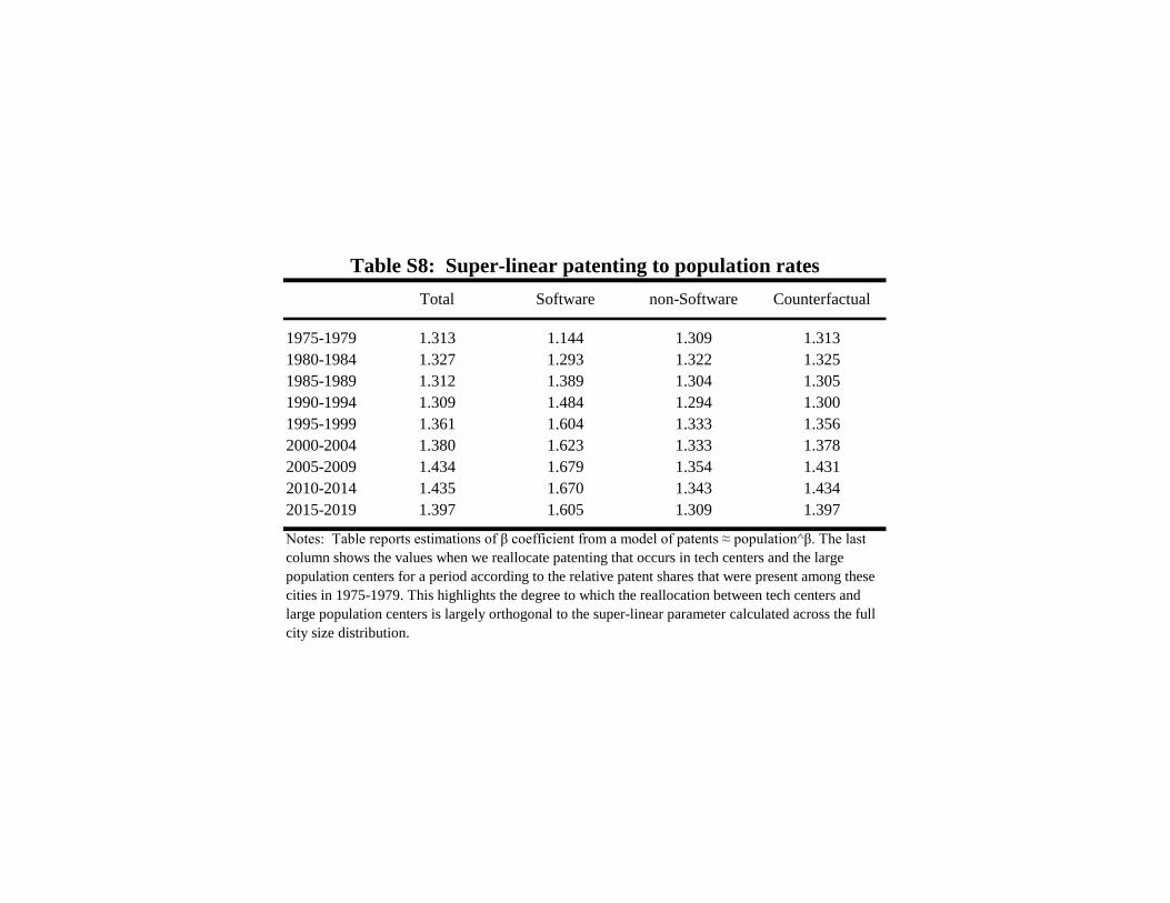
Total Software non-Software Counterfactual
1975-1979 1.313 1.144 1.309 1.313
1980-1984 1.327 1.293 1.322 1.325
1985-1989 1.312 1.389 1.304 1.305
1990-1994 1.309 1.484 1.294 1.300
1995-1999 1.361 1.604 1.333 1.356
2000-2004 1.380 1.623 1.333 1.378
2005-2009 1.434 1.679 1.354 1.431
2010-2014 1.435 1.670 1.343 1.434
2015-2019 1.397 1.605 1.309 1.397
Table S8: Super-linear patenting to population rates
Notes: Table reports estimations of β coefficient from a model of patents ≈ population^β. The last
column shows the values when we reallocate patenting that occurs in tech centers and the large
population centers for a period according to the relative patent shares that were present among these
cities in 1975-1979. This highlights the degree to which the reallocation between tech centers and
large population centers is largely orthogonal to the super-linear parameter calculated across the full
city size distribution.

F1 Precision Recall F1 Precision Recall F1 Precision Recall
Test Sample 0.861 0.846 0.877
Full Sample 0.843 0.788 0.906 0.801 0.679 0.976 0.894 0.874 0.915
1975-1979 0.682 0.600 0.789 0.667 0.514 0.948 0.832 0.798 0.870
1980-1984 0.753 0.638 0.918 0.661 0.497 0.986 0.824 0.722 0.959
1985-1989 0.806 0.750 0.871 0.784 0.655 0.978 0.881 0.929 0.839
1990-1994 0.842 0.802 0.885 0.786 0.667 0.958 0.885 0.885 0.885
1995-1999 0.935 0.953 0.918 0.851 0.763 0.964 0.872 0.911 0.836
2000-2004 0.902 0.855 0.955 0.862 0.768 0.982 0.931 0.893 0.973
2005-2009 0.846 0.792 0.908 0.856 0.759 0.982 0.930 0.891 0.972
2010-2014 0.912 0.870 0.958 0.898 0.815 1.000 0.950 0.935 0.966
Table S9: Diagnostics on software definitions
Notes: Table reports precision and recall estimates from an application of algorithms to a random sample of patents classified by authors as software related. We
randomly sampled 1600 patents from NBER Category 2 stratified across eight periods from 1976-79 to 2010-14. Within each period, we sampled 100 BH, 50 GV, and
50 other patents. One patent was sampled twice, and several could not be reliably assigned, resulting in a final sample of 1559 patents. A machine learning algorithm
was trained on 80% of data and then tested out-of-sample on the remaining 20%. F1=2*(precision*recall)/(precision+recall).
Bessen and Hunt (2007) Graham and Vishnubhakat (2013) Machine Learning Approach

Tech clusters Five largest Other 270 non-Urban
(6 cities) cities in 1980 cities areas
1975-1979 0.113 0.322 0.455 0.110
1980-1984 0.124 0.298 0.468 0.110
1985-1989 0.139 0.276 0.478 0.107
1990-1994 0.163 0.252 0.485 0.100
1995-1999 0.233 0.220 0.463 0.084
2000-2004 0.274 0.202 0.448 0.077
2005-2009 0.307 0.198 0.428 0.067
2010-2014 0.323 0.195 0.415 0.067
1975-1979 0.183 0.324 0.422 0.071
1980-1984 0.200 0.291 0.442 0.066
1985-1989 0.228 0.256 0.445 0.070
1990-1994 0.270 0.223 0.450 0.056
1995-1999 0.360 0.187 0.409 0.044
2000-2004 0.396 0.172 0.393 0.039
2005-2009 0.424 0.175 0.367 0.033
2010-2014 0.449 0.174 0.346 0.031
1975-1979 0.097 0.322 0.462 0.119
1980-1984 0.104 0.300 0.474 0.122
1985-1989 0.113 0.281 0.488 0.118
1990-1994 0.125 0.262 0.497 0.116
1995-1999 0.157 0.240 0.496 0.107
2000-2004 0.172 0.227 0.494 0.108
2005-2009 0.183 0.222 0.493 0.102
2010-2014 0.193 0.217 0.486 0.105
Table S10a: Concentration levels using GV definition
A. All patents
B. Software patents
C. non-Software patents
Notes: See Table S2. Software defined using Graham and Vishnubhakat (2013).

Tech clusters Five largest Other 270 non-Urban
(6 cities) cities in 1980 cities areas
1975-1979 0.113 0.322 0.455 0.110
1980-1984 0.124 0.298 0.468 0.110
1985-1989 0.139 0.276 0.478 0.107
1990-1994 0.163 0.252 0.485 0.100
1995-1999 0.233 0.221 0.463 0.084
2000-2004 0.274 0.202 0.448 0.076
2005-2009 0.310 0.198 0.427 0.066
2010-2014 0.337 0.189 0.413 0.062
2015-2019 0.342 0.186 0.410 0.061
1975-1979 0.160 0.348 0.424 0.068
1980-1984 0.195 0.315 0.432 0.057
1985-1989 0.231 0.293 0.413 0.063
1990-1994 0.278 0.260 0.411 0.052
1995-1999 0.364 0.217 0.378 0.041
2000-2004 0.400 0.195 0.368 0.037
2005-2009 0.425 0.190 0.349 0.036
2010-2014 0.459 0.179 0.327 0.035
2015-2019 0.461 0.176 0.328 0.036
1975-1979 0.109 0.320 0.457 0.114
1980-1984 0.117 0.296 0.471 0.116
1985-1989 0.128 0.274 0.486 0.112
1990-1994 0.141 0.250 0.499 0.110
1995-1999 0.182 0.222 0.496 0.100
2000-2004 0.209 0.205 0.489 0.097
2005-2009 0.227 0.203 0.482 0.087
2010-2014 0.238 0.197 0.482 0.083
2015-2019 0.242 0.195 0.480 0.083
Table S10b: Concentration levels using machine learning approach
A. All patents
B. Software patents
C. non-Software patents
Notes: See Table S2. Software defined using machine learning algorithm.

Tech clusters Five largest Other 270 non-Urban
(6 cities) cities in 1980 cities areas
1975-1979 0.113 0.322 0.455 0.110
1980-1984 0.124 0.298 0.468 0.110
1985-1989 0.139 0.276 0.478 0.107
1990-1994 0.163 0.252 0.485 0.100
1995-1999 0.233 0.221 0.463 0.084
2000-2004 0.274 0.202 0.448 0.076
2005-2009 0.310 0.198 0.427 0.066
2010-2014 0.337 0.189 0.413 0.062
2015-2019 0.342 0.186 0.410 0.061
1975-1979 0.183 0.317 0.425 0.076
1980-1984 0.211 0.288 0.442 0.058
1985-1989 0.263 0.254 0.420 0.063
1990-1994 0.319 0.217 0.411 0.053
1995-1999 0.426 0.192 0.349 0.033
2000-2004 0.452 0.174 0.344 0.031
2005-2009 0.471 0.178 0.326 0.025
2010-2014 0.505 0.173 0.297 0.024
2015-2019 0.502 0.172 0.301 0.026
1975-1979 0.112 0.322 0.455 0.111
1980-1984 0.123 0.298 0.468 0.111
1985-1989 0.136 0.276 0.480 0.108
1990-1994 0.156 0.254 0.488 0.102
1995-1999 0.213 0.223 0.475 0.089
2000-2004 0.247 0.206 0.464 0.083
2005-2009 0.275 0.202 0.448 0.074
2010-2014 0.296 0.193 0.440 0.071
2015-2019 0.302 0.190 0.438 0.070
Table S10c: Concentration levels using AI definition
A. All patents
B. AI-related patents
C. non-AI patents
Notes: See Table S2. AI-related patents defined using Giczy et al. (2021).

Software
Total Software share Total Software non-Software Total Software non-Software
1975-1979 197,897 4,968 2.51% 0.041 0.046 0.041 0.003 0.009 0.003
1980-1984 181,212 8,635 4.77% 0.037 0.039 0.037 0.003 0.007 0.003
1985-1989 214,539 15,172 7.07% 0.034 0.038 0.034 0.003 0.008 0.003
1990-1994 293,573 31,174 10.62% 0.032 0.044 0.031 0.005 0.017 0.004
1995-1999 443,669 87,172 19.65% 0.039 0.067 0.035 0.013 0.039 0.009
2000-2004 526,751 148,325 28.16% 0.045 0.071 0.038 0.020 0.046 0.013
2005-2009 515,688 201,201 39.02% 0.050 0.076 0.038 0.025 0.050 0.014
2009-2014 630,822 285,806 45.31% 0.057 0.092 0.038 0.032 0.065 0.014
2015-2019 494,057 246,593 49.91% 0.058 0.093 0.036 0.033 0.065 0.013
1975-1979 197,891 36,200 18.3% 0.041 0.050 0.039 0.003 0.009 0.003
1980-1984 181,181 37,687 20.8% 0.037 0.045 0.036 0.003 0.009 0.003
1985-1989 214,429 48,666 22.7% 0.034 0.044 0.033 0.003 0.011 0.003
1990-1994 293,466 77,971 26.6% 0.032 0.048 0.030 0.005 0.019 0.003
1995-1999 443,307 165,500 37.3% 0.039 0.071 0.030 0.013 0.042 0.005
2000-2004 525,416 238,531 45.4% 0.045 0.076 0.031 0.020 0.050 0.007
2005-2009 493,712 254,707 51.6% 0.049 0.079 0.031 0.024 0.052 0.008
2009-2014 303,394 154,871 51.0% 0.056 0.095 0.032 0.030 0.067 0.009
Notes: See Tables S3 and S10a.
Table S11a: Comparison of software and AI definitions
Patent count Herfindahl-Hirschman Index Ellison-Glaeser Index
A. Core results using Bessen and Hunt (2007) approach
B. Alternative definition from Graham and Vishnubhakat (2013)
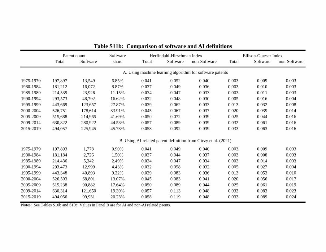
Software
Total Software share Total Software non-Software Total Software non-Software
1975-1979 197,897 13,549 6.85% 0.041 0.052 0.040 0.003 0.009 0.003
1980-1984 181,212 16,072 8.87% 0.037 0.049 0.036 0.003 0.010 0.003
1985-1989 214,539 23,926 11.15% 0.034 0.047 0.033 0.003 0.011 0.003
1990-1994 293,573 48,792 16.62% 0.032 0.048 0.030 0.005 0.016 0.004
1995-1999 443,669 123,657 27.87% 0.039 0.062 0.033 0.013 0.032 0.008
2000-2004 526,751 178,614 33.91% 0.045 0.067 0.037 0.020 0.039 0.014
2005-2009 515,688 214,965 41.69% 0.050 0.072 0.039 0.025 0.044 0.016
2009-2014 630,822 280,922 44.53% 0.057 0.089 0.039 0.032 0.061 0.016
2015-2019 494,057 225,945 45.73% 0.058 0.092 0.039 0.033 0.063 0.016
1975-1979 197,893 1,778 0.90% 0.041 0.049 0.040 0.003 0.009 0.003
1980-1984 181,184 2,726 1.50% 0.037 0.044 0.037 0.003 0.008 0.003
1985-1989 214,436 5,342 2.49% 0.034 0.047 0.034 0.003 0.014 0.003
1990-1994 293,473 12,999 4.43% 0.032 0.058 0.032 0.005 0.027 0.004
1995-1999 443,348 40,893 9.22% 0.039 0.083 0.036 0.013 0.053 0.010
2000-2004 526,503 68,801 13.07% 0.045 0.083 0.041 0.020 0.056 0.017
2005-2009 515,238 90,882 17.64% 0.050 0.089 0.044 0.025 0.061 0.019
2009-2014 630,314 121,650 19.30% 0.057 0.113 0.048 0.032 0.083 0.023
2015-2019 494,056 99,931 20.23% 0.058 0.119 0.048 0.033 0.089 0.024
Notes: See Tables S10b and S10c. Values in Panel B are for AI and non-AI related paents.
Table S11b: Comparison of software and AI definitions
Patent count Herfindahl-Hirschman Index Ellison-Glaeser Index
A. Using machine learning algorithm for software patents
B. Using AI-related patent definition from Giczy et al. (2021)