WILL THE MARSHALL LAWS OF DERIVED DEMAND STAND UP?

An Interpretation and Correction of Hicks� Elasticity Rules

bySalah El-Sheikh

Department of EconomicsSt. Francis Xavier University

Antigonish, NS B2G 2W5Canada

Phone: 902 867 3803Fax: 902 867 2448E-mail: selsheik@stfx.ca

ii

ABSTRACT

In his classic, The Theory of Wages, Hicks (1932) employed his innovative �elasticity of substitution� to

provide a mathematical �test� of Marshall�s four laws (rules) of derived demand, and concluded that all laws

(with a minor modification of the third) are �universally true�. Hicks� conclusion has since been granted

uncritical acceptance by researchers to date, and his formulation of the laws continues to be used in both

textbooks and empirical research.

The objective of this study is twofold: First, is to formulate a model that captures the essential features

of Hicks� Theory, then use it to demonstrate that his conclusions are a consequence of a flawed �testing�

method, and that none of his �rules� is �universally true�. Second is to develop a �testing� method rooted in

Marshallian comparative statics, and employ it to produce likely sets of sufficient conditions for Marshall�s four

�laws�.

The paper consists of six sections. Section B contains an interpretive version of the Hicksian model,

and an explication of his rule-testing method and results. In section C, a Marshallian testing method is

developed, then employed to examine rules II and III (in Section D) and rules I and IV (in Section E). Finally

the paper ends with concluding remarks in Section F.

[JEL D00 , D33 , J23]

1

A. INTRODUCTION

Modern theory of input demand goes back to the path-breaking work of Alfred Marshall, the co-founder

and architect of Neoclassical Economics.1 In his magnum opus, Principles of Economics, Marshall (1890)

coined the general term �derived demand�, invented the concept of (price) �elasticity�, and investigated the

determinants of the �elasticity of derived demand� to answer questions about the distribution of income among

factor owners. In Marshallesque style, he illustrated his theory by means of a socially important phenomenon,

�labour disputes� and �trade-union conflicts�,2 to examine �the conditions under which an enforced increase in

the wage rate� will favour �the real income of workpeople, and so of the poor�, as his renowned disciple and

expositor Pigou (1932: p. 681) put it.3 And to answer the question, he formulated his general model (of a

competitive industry), verbally in the text and mathematically in appendix note XIV, as it was typical of

Marshall, the expert mathematician.4

Marshall discovered four �conditions�, those being �the conditions that determine whether the demand

for the services of any assigned group of workpeople is likely to have a high elasticity or a low one�, again in

the words of Pigou (1932: pp. 682f) who formulated the canonical statement of Marshall�s elasticity

conditions:5

I. �the demand for anything is likely to be more elastic, the more readily substitutes for that thingcan be obtained�;

II. �the demand for anything is likely to be more elastic, the more elastic is the demand for anyfurther thing which it contributes to produce�;

III. �the demand for anything is likely to be less elastic, the less important is the part played by thecost of that thing in the total cost of some other thing, in the production of which it isemployed�;

IV. �the demand for anything is likely to be more elastic, the more elastic is the supply of co-operant agents of production.� [emphasis added]

Again, characteristic of Marshallian method, to demonstrate the validity of these conditions, he opted

for another example (knife-handles) that simplified the production process into one of fixed production

coefficients. The demonstration of conditions II � IV was carried out in footnotes, only graphically, and the

mathematical model was relegated to appendix note XV whereby his seminal elasticity formula was derived.6

2

Of the four conditions, only the third � presumably because of its paradoxical nature � intrigued many

economists including Henderson (1922: pp. 59f) who coined the phrase �the importance of being unimportant�

to capture its essence and � in the process � highlight a research �puzzle� à la Kuhn.7 In the footsteps of

Marshall (and Pigou), but forty-two years later, Hicks (1932: pp. 112-13) published The Theory of Wages and,

in Chapter VI, set out to investigate �one of the most venerable of economic problems�: �Is economic progress

likely to raise or lower the proportion of the National Dividend which goes to labour?�;8 and, like them, to

address this question, he examined the elasticity of derived demand. Yet, unlike Marshall (1920: p. 317)

analysis of a strike, �the period over which the disturbance extends being short� and the �coefficients of

production� may be assumed constant,9 the Hicksian question, being inherently about long-run equilibrium,

required a model like Marshall�s general model of appendix note XIV.

Hence, in the spirit of Marshall (1920: pp. 141n, 295-99) �principle of substitution�, Hicks deployed

the Marshallian general concept of (function) �elasticity� to measure the degree of technical substitutability

between labor and other inputs in his innovative σ, the �elasticity of substitution�,10 a fundamental property of a

production function explicitly introduced into his Marshallian model.11 And accepting the views of Walras and

Wicksell in favour of Wicksteed doctrine of product exhaustion, Hicks (1932: pp. 233f) assumed constant

returns to scale (for the industry) and adopted a linearly homogenous production function, an assumption that

was implicitly made by Marshall in his knife-handles model (by virtue of its Leontief technology).12

Mindful that �economists have generally been content to use Marshall�s rules, without making them the

subject of any further investigation�, Hicks (1932: p. 24) expressed concern that their being �used in formally

non-mathematical arguments� �is dangerous�; and �instead of merely accepting Marshall�s conclusions�

(including condition I, which was not demonstrated as yet), he employed his Marshallian model to �examine

their mathematical foundation� in the Appendix (of Chapter VI: pp. 241-46). Hicks� examination produced a

generalization of Marshall�s elasticity formula (that included σ) which he used to �test� Marshall�s �four rules�

(by means of partially differentiating the elasticity of derived demand, λ). Hicks� mathematical �testing� gave

three principal results and an overall conclusion: 1) a novel mathematical �demonstration� of rule I by means of

σ; 2) confirmation of rules II and IV in the presence of technical substitution; 3) rule III is valid if and only if

3

the elasticity of output demand η > σ: �It is �important to be unimportant� only when the consumer can

substitute more easily than the entrepreneur�.

Hicks� overall conclusion was that �The first, [second] and fourth rules are universally true. But the

[third] rule is not universally true� [emphasis added].13 Notice the subtle change in tone, one that appears to

have gone unnoticed by researchers afterwards. The previously stated Marshall/Pigou �conditions� are mere

synthetic (empirically likely) propositions, whereas the Marshall/Hicks �rules� are analytic propositions that are

�universally true� according to Hicks.14

The subtle change in the logical status of Marshall�s �conditions� � in effect a metamorphosis from

�likely determinants� into �universal rules� � was not noted by the eminent reviewer of The Theory of Wages,

Shove (1933: p. 261), who praised Hicks for �ingeniously . . . combining [σ] into a formula and, in one respect,

modifying the four rules laid down by Marshall�. 15 The tenor of his laudatory statement prevailed, and � with

the notable exception of Allen (1938)16 � systematic exploration of Marshall�s conditions ceased for thirty more

years until Bronfenbrenner (1961) broke the silence.17 In the meantime, the status of Marshall�s conditions was

again elevated from �rules� into �laws�, and the third-condition �puzzle� was reincarnated into a �Hicks�

paradox� that continued to intrigue researchers.18

Noting that �attention has . . . shifted� away because of �the possible impression that the problem was

solved�, Bronfenbrenner (1961: p. 254) signaled a �return to the historically prior and more obviously policy-

relevant problem of the market elasticities of derived demand�. He reviewed Marshall�s, Hicks� and Allen�s

�solutions� to the problem,19 used their respective elasticity formulas, and employed the Hicksian method of

�testing� to reexamine Marshall�s �four laws�.20 Bronfenbrenner (1961: pp. 257 f) �confirmed� all of Hicks�

findings regarding the �laws�, but pointed out that the �plausibility of the exceptions to Marshall�s third rule has

yet to be demonstrated convincingly or even completely in literary terms�.21 This last statement prompted a

�Comment� by Hicks (1961), primarily aiming at providing that �convincing literary demonstration�.22 No such

�literary demonstration� has ever been requested or provided for the other three rules.

The Bronfenbrenner/Hicks exchange and Hicks (1963) appear to have had spawned a spate of

theoretical studies on derived demand in general and its elasticity in particular. Notable for our purposes are the

works that reexamined the Marshall/Hicks laws � all used the Hicksian method of testing.23 Friedman (1962:

4

pp. 153f) employed Marshall�s knife-handles model to provide a geometric �demonstration� of the three last

laws. Muth (1964) used a similar model to that of Hicks, and derived elasticity formulas for input demand and

output supply.24 Bronfenbrenner (1971) expanded on his previous work and claimed that �Hicks� exception to

Marshall�s third rule . . . is a blind alley . . . [because it requires] that the share of an input be negative� (p. 149).

Ferguson (1971: pp. 235 f) derived Allen�s elasticity formula, and confirmed Hicks� findings.25 Sato and

Koizumi (1970) expanded the Allen (1938) multi-input model (endogenizing the prices of cooperant inputs) and

derived Hicks-like elasticity rules, again confirming all Hicksian findings.26 On the other hand, Maurice (1972)

developed the Allen multi-input model to endogenize the number of firms, and confirm Hicks� findings except

that � he found � �it is always �important to be unimportant� . . . [because] Hicks caveat does not apply� (p.

1272). Finally, the opposing results concerning the third rule were reconciled by Maurice (1975) who aptly

demonstrated that the dispute was a consequence of alternative specifications of the elasticity of substitution:

Hicks� direct elasticity caused his �caveat� to be confirmed, whereas Allen�s partial elasticity caused it to be

refuted. And with this reconciliation, theoretical research on Marshall�s elasticity conditions came to an end.27

It is noteworthy that, all along, Hicks� findings on Marshall�s first, second and fourth conditions have

never been called into question. And with the third-rule dispute resolved, the Marshall/Hicks �rules/laws� have

become �universally� accepted �truths� about derived demand, as Hicks intended them to be. Currently they

constitute the canon in textbook treatments and in empirical research, especially on labour demand.28

The objective of this study is twofold: First, is to formulate a model that captures the essential aspects

of Hicks� Theory, then use it to demonstrate that his conclusions are a consequence of a flawed �testing�

method, and that none of his �rules� is �universally true�. Second is to develop a �testing� method rooted in

Marshallian comparative statics, and employ it to produce �likely� sets of sufficient conditions for Marshall�s

four �laws�. And although the study is concerned with theory, the historical texts of principal contributors are

analyzed primarily to shed light on the current state of input-demand theory.

The paper consists of six sections. Section B contains an interpretive version of Hicks (1932) model,

and an explication of his rule-testing method and results. In section C, a Marshallian testing method is

developed, then employed to examine rules II and III (in Section D), and rules I and IV (in Section E). Finally

the paper ends with concluding remarks in Section F.

5

��

���

θδγβ=θδγβ=

θδγβ=θδγβ=θδγβ=

. ) , , , v(w; v; ) , , , P(w; P; ) , , , Q(w; Q ; ) , , , K(w; K ); , , , L(w; L

)7(**

***

B. HICKS MODEL AND RULE TESTING: AN INTERPRETATION

The following formulation captures the salient features of the Hicks (1932) industry model and utilizes

its underlying conceptual framework.29 The industry is characterized by the following C2, quasiconcave

production function:30

(1) Q = F(L, K; δ, θ) ; FL, FK > 0 ; FLL, FKK < 0,

where Q, L and K are flows of output, labor and capital services respectively; δ and θ are distribution and

substitution parameters representing � if changed � alternative types of Hicks� �autonomous invention� (later, to

be specified).31 F(.) is also homogeneous of degree one such that,

(2) F(.) ≡ FLL + FKK ; FLL = −(K/L)FLK ; FKK = −(L/K)FLK ;

(3) FLLL2 + FKK K2 + 2 FLK LK = 0 , σ = FLFK/QFLK > 0 ;

where σ is Hicks� elasticity of substitution.

Operating in competitive markets, the industry applies the following profit-maximizing rules in

determining its input demand:

(4) w = P FL(L, K; δ, θ); v = P FK(L, K; δ, θ);

where P, w and v are the output price, wage and rental rates respectively. And while w is exogenous, the

market-clearing conditions of capital services and the industry�s output are:

(5) K = Ks ; Ks = S(v; β) , S′ > 0 ;

(6) Q = QD ; QD = D(P; γ) , D′ < 0 ;

the supply and demand functions, S(.) and D(.), are C2, and the autonomous parameters β and γ determine their

respective price elasticities.

Model�s Comparative Statics and Hicks� Elasticity Formula:

Under model�s assumptions, the implicit function theorem ensures that the simultaneous-equation

system in (1), (4), (5) and (6) uniquely defines an equilibrium solution for the endogenous variables (L*, K*,

Q*, P*, v*) in terms of the exogenous variable w and parametric data (the autonomous β, γ, δ, θ) according to

the following set of implicit functions:

6

. 0 ) , , , e(w; K(.) / v(.)(.)S e and 0, ) , , , (w; Q(.) / P(.) (.)D >θδγβ=′=>θδγβη=′−=η

; /YY /Y,Y vK; Y wL, Y ,Y Y PQ Y KKLLKLKL ====+== αα

. 0 )] (e ) (eQ[Y e] [QY D KL2

KL2 >η+α+σ+ασ=+ηα+σασ=

; 0 )]} ( e) [( / )e] ( e) ({[ Den} /])e( e) ((L/w){[ Den} / )] e( (L/w){[ w)/L(

LLLw

KLKL*

<σ−ηα−+ησ−ηα++ησ−=ε⇔σ+ηα−η+σα−=σα+ηα+ησ−=∂∂

; 0 1 ; Den} / e) ({ Den} / e) ((P/w){ w)/P( (18) wpLwpL

* >ε>+σα=ε⇔+σα=∂∂

[ ] [ ][ ] [ ] [ ]�

��

θδ≡γβ≡θδ≡θδ≡

. , K(.); L(.), F P(.); D ; v(.); S K(.); , K(.); (.),L F P(.) (.) v; , K(.); L(.),F P(.) w

)8( KL

where; 0 0 /wLY

w/Pw/K

w/L

Q v weKQ YeY wKe

LQ vL Y (14)

*

*

*

L

K

���

�

�

���

�

� σ=

���

�

�

���

�

�

∂∂

∂∂

∂∂

���

�

�

���

�

�

ησσ−−σ−

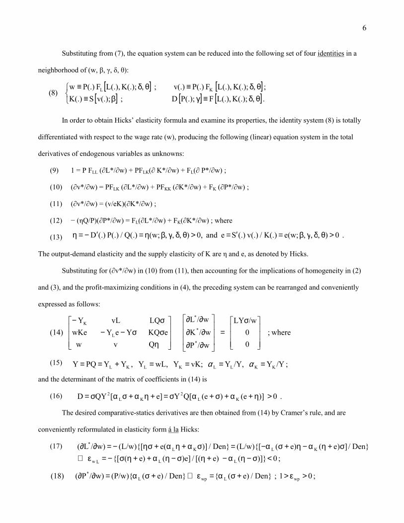
Substituting from (7), the equation system can be reduced into the following set of four identities in a

neighborhood of (w, β, γ, δ, θ):

In order to obtain Hicks� elasticity formula and examine its properties, the identity system (8) is totally

differentiated with respect to the wage rate (w), producing the following (linear) equation system in the total

derivatives of endogenous variables as unknowns:

(9) 1 = P FLL (∂L*/∂w) + PFLK(∂ K*/∂w) + FL(∂ P*/∂w) ;

(10) (∂v*/∂w) = PFLK (∂L*/∂w) + PFKK (∂K*/∂w) + FK (∂P*/∂w) ;

(11) (∂v*/∂w) = (v/eK)(∂K*/∂w) ;

(12) − (ηQ/P)(∂P*/∂w) = FL(∂L*/∂w) + FK(∂K*/∂w) ; where

(13)

The output-demand elasticity and the supply elasticity of K are η and e, as denoted by Hicks.

Substituting for (∂v*/∂w) in (10) from (11), then accounting for the implications of homogeneity in (2)

and (3), and the profit-maximizing conditions in (4), the preceding system can be rearranged and conveniently

expressed as follows:

(15)

and the determinant of the matrix of coefficients in (14) is

(16)

The desired comparative-statics derivatives are then obtained from (14) by Cramer�s rule, and are

conveniently reformulated in elasticity form á la Hicks:

(17)

7

.) , , , k(w; P(.)Q(.) / wL(.)k and ), , , , (w; (.)F(.)F / (.)F (.)F LKKL θδγβ==θδγβσ==σ

; iff 0 Den} / )e ({

Den} / ]e) ()e( (K/w){[ Den} / )e ((K/w){ w)/K( (19)

LwK

LLL*

η<>σ

<>η−σα=ε⇔

σ+ηα+η+σα−=η−σα=∂∂

;1 ; iff 0 Den} / ) ({ Den} / ) ((v/w){ w)/v( (20) wvLwvL* <εη

<>σ

<>η−σα=ε⇔η−σα=∂∂

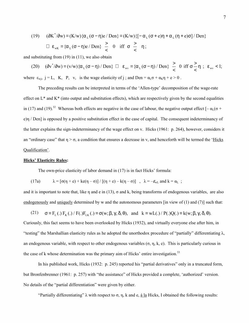
and substituting from (19) in (11), we also obtain

where εwj, j = L, K, P, v, is the wage elasticity of j ; and Den = αLσ + αKη + e > 0 .

The preceding results can be interpreted in terms of the �Allen-type� decomposition of the wage-rate

effect on L* and K* (into output and substitution effects), which are respectively given by the second equalities

in (17) and (19).32 Whereas both effects are negative in the case of labour, the negative output effect [� αL(σ +

e)η / Den] is opposed by a positive substitution effect in the case of capital. The consequent indeterminancy of

the latter explains the sign-indeterminancy of the wage effect on v. Hicks (1961: p. 264), however, considers it

an �ordinary case� that η > σ, a condition that ensures a decrease in v, and henceforth will be termed the �Hicks

Qualification�.

Hicks� Elasticity Rules:

The own-price elasticity of labor demand in (17) is in fact Hicks� formula:

(17a) λ = [σ(η + e) + ke(η � σ)] / [(η + e) � k(η � σ)] , λ = �εwL and k = αL ;

and it is important to note that, like η and e in (13), σ and k, being transforms of endogenous variables, are also

endogenously and uniquely determined by w and the autonomous parameters [in view of (1) and (7)] such that:

(21)

Curiously, this fact seems to have been overlooked by Hicks (1932), and virtually everyone else after him, in

�testing� the Marshallian elasticity rules as he adopted the unorthodox procedure of �partially� differentiating λ,

an endogenous variable, with respect to other endogenous variables (σ, η, k, e). This is particularly curious in

the case of k whose determination was the primary aim of Hicks� entire investigation.33

In his published work, Hicks (1932: p. 245) reported his �partial derivatives� only in a truncated form,

but Bronfenbrenner (1961: p. 257) with �the assistance� of Hicks provided a complete, �authorized� version.

No details of the �partial differentiation� were given by either.

�Partially differentiating� λ with respect to σ, η, k and e, á la Hicks, I obtained the following results:

8

where, Den = (η + e) � k(η � σ) .

In order to obtain the exact Hicks/Bronfenbrenner �partial derivatives�, two sets of conditions must be

met. First is the zero conditionals contained in (22)-(25) respectively; they seem to be assumed implicitly, but

were never justified vis á vis (13) and (21). These conditionals, however, are met if their respective elasticity

terms are assumed autonomous, an assumption that was not made by Hicks and others34. Second, the

derivatives (∂k/∂σ), (∂k/∂η), and (∂k/∂e) must also equal zero, an untenable assumption on Hicks� own terms,

given (21) and especially because, like λ itself, k is a transform of L*.35 If these two sets of conditions are

granted however, Marshall�s four �rules� will have become only conditionally validated, with the third rule in

(24) also requiring the Hicksian qualification (η>σ) and the fourth requiring that η ≠ σ as well. But this

conditional validity runs counter to both the spirit and letter of the model, and especially to the above-mentioned

claim by Hicks (1932: p. 245) that the �first, [second] and fourth of these expressions [22, 23, 25] are always

positive� so that the �first, [second] and fourth rules are universally true� (emphasis added).

In any event, only under the above-mentioned conditions that Hicks (1961: p. 262) can also make the

claim (for his �partial derivatives�) that: �There is, I think, no doubt that the mathematics were right; no one has

found anything wrong with them in nearly 30 years�.36 Otherwise, his unusual method of �partially

differentiating� the endogenously determined λ with respect to the other endogenous �variables� σ, η, k and e

cannot be mathematically justified by the implicit function theorem, the cornerstone of comparative statics37.

; 0 }Den / e)]k/e)( e)( )( ( ) k)( {[k(1 e)/(

then0, e)/( e)/( If (25) ; iff 0 }Den / k)]k/e)( e)( )( {[( k)/(

then0, k)e/( k)/( k)/( If (24)

, 0 }Den / )]k/e)( e)( )( ( ) {[k(e )/(

then0, )e/( )/( If (23)

; 0 }Den / )]k/e)( e)( )( ( e) k)( {[(1 )/(

then0, )e/( )/( If (22)

22

2

22

22

<>∂∂+σ+ησ−η+σ−η−=∂λ∂

=∂η∂=∂σ∂σ>η>∂∂+σ+ησ−η=∂λ∂

=∂∂=∂η∂=∂σ∂<>η∂∂+σ+ησ−η+σ+=η∂λ∂

=η∂∂=η∂σ∂<>σ∂∂+σ+ησ−η++η−=σ∂λ∂

=σ∂∂=σ∂η∂

9

C. HICKS� RULES TESTED: A MARSHALLIAN METHOD

In principle, the object of Hicks� testing procedure was to conduct Marshallian �hypothetical� �thought

experiments�, one for each elasticity rule.38 Yet the failure to explicitly classify variables into endogenous and

exogenous has resulted generally in a vague specification of the autonomous causes of change and their

correlative ceteris paribus assumptions, in an equilibrium context. The result has been a great deal of confusion,

paradox and controversy in the literature on rule III, and � I think � an unjustified and uncritical consensus on

the analytic validity and �universality� claimed by Hicks for the other three elasticity rules.39

It is important to recall that (17a), Hicks ingenious formula, is in the nature of an identity that represents

the unique equilibrium relation among its endogenously determined elements (λ, σ, η, k, e), given the model�s

explicit data (w, β, γ, δ, θ) and other parametric features of its structural equations:40

(17b) λ = � (∂L*/∂w)(w/L*) = λ(σ, η, k, e) .

�Partially� differentiating λ with respect to say σ (η, e, or k) á la Hicks is akin to �arm-twisting� the �organic

structure� of this unique relation, thus changing the �structural properties� of equilibrium; and this can

legitimately occur only if one (or some) of the model�s parameters is exogenously changed. Mathematically,

what happens in effect is tantamount to treating σ (η, e or k) �as if� exogenous, and implicitly �endogenizing�

one (or more) of the structural parameters to accommodate adjustment to a new equilibrium. The problem with

Hicks� �partial derivatives� is that it is not clear which parameter(s) is being �endogenized� because σ (η, e or k)

is determined by the same test conditions w, β, γ, δ, θ and other parametric data of model�s equations.

This problem is compounded by assuming also that ∂k/∂σ (∂k/∂η or ∂k/∂e) = 0, an assumption that can

be met in two alternative scenarios. The first is to opt for a special case such as a Cobb-Douglas technology

whereby k is constant (σ = 1). But this particular special case would be inadmissible to Hicks for two reasons:

1) it negates his �universality� claim; 2) being necessarily equal to unity, σ is structurally unchangeable and the

testing of Rule I, Hicks� primary contribution, is not possible. The second scenario is to design two-tier

experiments whereby the �exogenous� change in σ (η or e) is conjoined with measured structural change (some

other parametric shift) to �sterilize� the endogenously induced change in k, and produce a zero derivative. But

again this type of experiment is problematic, not only because there are as many experiments as the model�s

parameters and their possible combinations, but also because of the consequent difficulty in identifying an exact

10

and coherent cæteris paribus clause for �the experiment�, in view of the endogeneity of other elasticities (η and e

for instance). Hicks� way out of this difficulty, it seems, was his implicit assumption that η and e were

(exogenous) parameters (in case of Rule I for instance), and this again delimits Hicks� claimed �universality�.

It seems to me that the problem arises primarily from a conceptual flaw in Hicks� testing method:

treating k �as if� of the same nature as σ, η and e (in his �partial� differentiation). For although all are

endogenously determined in principle, k differs fundamentally from the rest. Unlike σ, η and e, which aim at

measuring the behavioral responses that inhere in their respective structural equations (and may be treated as test

conditions), k is a side construct, an after-thought in the architecture of neoclassical theory, motivated by a

social interest in income distribution. As such, in general , k does not �subsist� in any particular structural

equation, although it can be directly manipulated by exogenous changes in w, δ or Ks (because, k = wL/PQ = 1 �

vK/PQ).

The preceding conceptual difference calls for a distinction between the direct (autonomous) changes in

k and the indirect (endogenous) changes which are induced by autonomous changes in σ, η or e, among other

things. The latter is part of the adjustment process towards new equilibria, and cannot be arbitrarily

�suppressed� (as Hicks� �partial� differentiation does) without forcing on the model a kind of structural change

in some equation or the other.

The upshot of the preceding distinction is the exclusion of (indirect changes in) k from the cæteris

paribus assumptions involved in testing rules I, II and IV. After all, generally, k is not a �parameter� that can be

�partially� differentiated into zero, arbitrarily, given (21). To put it in the exceptionally apt language of

Marshall (1920: p. 304), k is not one of those �disturbing causes, whose wanderings happen to be

inconvenient�, and therefore it should not be �segregated� in the �pound of cæteris paribus”.41 In fact, a careful

reading of Marshall�s own geometric �demonstration� of his last three conditions points to this direction.42 I will

adopt this distinction in the design of my �test experiments� for all rules (including the third) within the spirit of

the Marshallian model and its Hicksian elaboration. In so doing, and in order to produce concrete analytical

results, I will also mostly adopt Hicks� practice of treating as (cæteris paribus) parameters all elasticities except

the rule�s object (viz. η and e in rule I). The implementation of this testing method is undertaken in two steps.

11

The first produces the Hicks-like derivatives of λ stated in (22)-(25) whereas, in the second, the derivatives of k

in these equations are computed, and the status of their corresponding Marshallian rules is examined.

In order to save space, the first step is briefly worked out here, but only for rule I as an illustration. That

is, for obtaining (22), we �engineer� a substitution-enhancing technological change, a Hicksian �autonomous

invention�, by means of θ, which is directly mediated into the system via σ.43 And to isloate the effect of σ on λ

in this �experiment�, we control the other �structural� determinants of both by: 1) assuming, like Hicks, that η

and e are given (as parameters), and 2) specifying θ so as to ensure its �structural neutrality� as regards income

distribution (Hicks neutrality). Then, differentiating λ(.) with respect to θ, Hicks� rational function in (17a)

gives:

(26) (∂λ/∂σ)(∂σ/∂θ) = {[Den.(∂Num/∂θ) � Num.(∂Den/∂θ)] / Den2} , where

(26a) (∂Num/∂θ) = (∂σ/∂θ){[(η + e) � ke] + e(η � σ)(∂k/∂σ)}, and

(26b) (∂Den/∂θ) = (∂σ/∂θ){k � (η � σ)(∂k/∂σ)}.

Substituting in (26) from (26a), (26b), and for the numerator (Num) and denominator (Den) of λ, then cancelling

(∂σ/∂θ) and rearranging, we obtain (22) above.

Similarly, (24) is obtained by means of another type of �autonomous� innovational activity, a labor-

biased but substitution-neutral change in δ, and (23) and (25) by η- and e- augmenting changes in γ and β

respectively. In the process, analogous �controls� are applied in each �experiment� to ensure an appropriate

ceteris-paribus clause for each rule. The formulation of these controls, which palys a critical role in

determining the derivatives of k, is pursued below on a rule-by-rule basis as part of the second step.

Before embarking on this task, the derivatives (∂λ/∂σ), (∂λ/∂η), (∂λ/∂k) and (∂λ/∂e) in (22)-(25) merit at

least four pertinent observations. First, all these derivatives are sign indeterminate. That is, even with the

somewhat restrictive assumptions made above, none of Marshall�s elasticity rules seems to be �universally

true�. Second, only (24), Hicks� result on rule III, remains intact, including the so-called Hicks� �caveat� or

�paradox�, which hinges on (η � σ). That is, the validity of rule III is still predicated on Hicks� Qualification (η

> σ) being a necessary and sufficient condition. Third, the source of indeterminancy, the expression (η � σ)(η +

e)(σ + e), reproduces itself in all equations as a coefficient of their respective k-derivatives; each derivative

measuring the effect of say a changed σ (η, k or e) on labour�s share (k) in average cost (or output price). As

12

such, the expression (σ � η)(η + e)(σ + e) determines (via modifying the output and substitution effects of w on

K*) both the direction and the extent to which the induced change in k modifies (v/w), which in turn modifies

the substitution effect of w on L.44 Fourth, because the indeterminancy in rules I, II and IV is compounded by

both the signs and magnitudes of the k-derivatives, ironically, the validity of Marshall�s third law, the subject of

much controversy in the past,45 appears to be the least problematic among his four laws, as regards the Hicksian

claim of �universality�. Hence, I deal with it first.

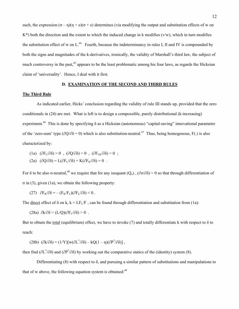
D. EXAMINATION OF THE SECOND AND THIRD RULES

The Third Rule

As indicated earlier, Hicks� conclusion regarding the validity of rule III stands up, provided that the zero

conditionals in (24) are met. What is left is to design a compossible, purely distributional (k-increasing)

experiment.46 This is done by specifying δ as a Hicksian (autonomous) �capital-saving� innovational parameter

of the �zero-sum� type (∂Q/∂δ = 0) which is also substitution-neutral.47 Thus, being homogenous, F(.) is also

characterized by:

(1a) (∂FL/∂δ) > 0 , (∂Q/∂δ) = 0 , (∂FLK/∂δ) = 0 ;

(2a) (∂Q/∂δ) = L(∂FL/∂δ) + K(∂FK/∂δ) = 0 .

For δ to be also σ-neutral,48 we require that for any isoquant (Qo) , (∂σ/∂δ) = 0 so that through differentiation of

σ in (3), given (1a), we obtain the following property:

(27) ∂FK/∂δ = � (FK/FL)(∂FL/∂δ) < 0 .

The direct effect of δ on k, k = LFL/F , can be found through differentiation and substitution from (1a):

(28a) ∂k/∂δ = (L/Q)(∂FL/∂δ) > 0 .

But to obtain the total (equilibrium) effect, we have to invoke (7) and totally differentiate k with respect to δ to

reach:

(28b) (∂k/∂δ) = (1/Y)[w(∂L*/∂δ) � kQ(1 � η)(∂P*/∂δ)] ,

then find (∂L*/∂δ) and (∂P*/∂δ) by working out the comparative statics of the (identity) system (8).

Differentiating (8) with respect to δ, and pursuing a similar pattern of substitutions and manipulations to

that of w above, the following equation system is obtained:49

13

. )Q/P(

)/F)(e/FKY ()/F)(/F(LY

/P/K

/L

Q v weKQ YeY wKe

LQ vL Y

Kk

LL

*

*

*

L

K

���

�

�

���

�

�

δ∂∂δ∂∂σ

δ∂∂σ−=

���

�

�

���

�

�

δ∂∂

δ∂∂

δ∂∂

���

�

�

���

�

�

ησσ−−σ−

; 0 )/F( e]} k) (1 [k / e) (){(L/F )/L( (30) LL* >δ∂∂+η−+σ+ησ=δ∂∂

(29)

Accounting for (1a) and (27) in the RHS column of (29), the following comparative-statics results can be found

(by Cramer�s rule):

Finally, substituting from (30) and (31) for (∂L*/∂δ) and (∂P*/∂δ) in (28b), the total effect on k is found:

And on the basis of the foregoing analysis, a conclusion is drawn in the following:

Theorem (1): Assuming σ, η and e are autonomous, and k is driven by δ, a Hicks �capital-saving� (zero sum) type of technological change that is also �substitution-neutral� such that (27)holds, then rule III applies (∂λ/∂k > 0) iff η > σ .

The Second Rule

Unlike the third rule, (23) suggests that Hicks qualification alone does not help determining the validity

of rule II unless (∂k/∂η) is known. Hence, an η-augmenting experiment is specified: an autonomous change in

output demand such that,50

(6a) (∂QD/∂γ) < 0 , (∂2QD/∂γ∂P) ≤ 0 .

That γ is structurally η-augmenting is ascertained by recalling (6) and (13), then recognizing that, at some initial

price (P),

(6b) η = �D′(P, γ) . P/D(P, γ) = η*(γ; P) ,

so that the direct effect on η, which can be found by partial differentiation, is

(32) (∂η/∂γ) = � (η/Q)(∂QD/∂γ) � (P/Q)(∂2QD/∂γ∂P) > 0 .

To compute the direct effect of the increased η on QD (at the initial price), having found η*(.) is

monotonically increasing by (32), we infer from (6b) and (6) that

. 0 )/Fe]}( k) (1 [k / k){F/P( )/P( )31( LL

* <δ∂∂+η−+σσ−=δ∂∂

. 0 )/Fe]}( k) (1 [k / k] k) (1 e){[/F(k )k/( )c28( LL >δ∂∂+η−+σ+η−+σ=δ∂∂

14

. )/QP(

0 0

/P/K

/L

Q v weKQ YeY wKe

LQ vL Y

D*

*

*

L

K

���

�

�

���

�

�

η∂∂

=���

�

�

���

�

�

η∂∂

η∂∂

η∂∂

���

�

�

���

�

�

ησσ−−σ−

; 0 e]} k) (1 [k / e) {( e]} k) (1 [k / e) ){((L/ )/L( )37( L* <+η−+σ+σ−=ε⇔+η−+σ+ση−=η∂∂ η

; 0 e]} k) (1 [(k / k) {(1 e]} k) (1 [k / k) ){(1(P/ )/P( )38( P* <+η−+σ−−=ε⇔+η−+σ−η−=η∂∂ η

. 1 iff 0 e k k) k)(k/k/( (35a)><σ

<>]}+η) − (1 +σ[ / σ− )(1 − {(1η = )η∂∂

(6c) η = η*(γ; P) ⇔ γ = γ(η; P) ; and that QD = D*(η; P) ,

then obtain the following identity:

(33) QD = D(γ; P) ≡ D*[η*(γ; P) ; P]

which gives (by differentiation):

(34) (∂QD/∂η) = (∂QD/∂γ) / (∂η/∂γ) < 0 .

In order to obtain concrete analytical results regarding rule II, I will employ a simplified, albeit

common, type of demand shift whereby (∂2QD/∂γ∂P) = 0,51 such that, by substitution from (32), (34) becomes:

(34a) (∂QD/∂η) = � (Q/η) < 0 .

Computation of (∂k/∂η): To find the (equilibrium) change in k due to increased η, k is differentiated with

respect to γ [invoking (7), (6b) and (32)]. Cancelling (∂η/∂γ), imposing (34a) and rearranging, we obtain:

(35) (∂k/∂η) = (1/Y)[w(∂L*/∂η) � kQ(1 � η)(∂P*/∂η)] + (k/η) .

The total derivatives (∂L*/∂η) and (∂P*/∂η) are then found from comparative statics of the model.

Again, totally differentiating (8) with respect to γ, cancelling (∂η/∂γ) from resulting equations, then

similarly substituting and rearranging (as with w above), we obtain:

(36)

Upon substitution for (∂QD/∂η) from (34a), the comparative-statics derivatives are found from (37) (by Cramer�s

rule) and reformulated as:

where, εηj , j = L, P, is the η-elasticity of j.

The total derivative of k and its sign are finally obtained by substitution in (35) for (∂L*/∂η) and

(∂P*/∂η) from (37) and (38), and rearranging:

Status of Rule II: In order to assess the validity of this rule, (35a) is used to substitute for (∂k/∂η) in

(23). Rearranged, the numerator of (23) becomes:

15

. 1 Ziff 0 Num iff 0 )/( (40)

positive, is (23) ofr denominato thebecause Therefore,

. k e k) (1k)e (1 k) 1(

e 1 Z, ] Z 1[) k(e Num )39(

22

222

2

><

<>

<>η∂λ∂

��

���

�

σ++η−−+η−

��

�

�

+σ−σ

���

�

�

ησ−η=−σ+=

Evidently, the Hicksian (determinate) derivative obtains if Z2 = 0 : σ = η or σ = 1 . Yet, because Z2

can assume any value, positive or negative, on the real line, I will consider three situations under which Z2 < 1,

thereby providing alternative sufficient conditions for the validity of Rule II:

(i) Hicks Qualification case: If η > σ, then (η � σ)/η is a positive fraction. And because the bracketed

expression of Z2 in (39) is invariably a positive fraction and [(σ � 1) / (σ + e)] < 1, it follows that Z2 < 1.

(ii) A General Case: Irrespective of Hicks Qualification, again because the bracketted expression of Z2 is

a positive fraction, and since by (40) (∂λ/∂η) ≤ 0 iff Z2 ≥ 1, then

(41) Z2 ≥ 1 � x > 1 , and x ≤ 1 � Z2 < 1 , x = (η � σ)(σ � 1) / η(σ + e) ; and

(42) {x ≤ 1 ⇔ e ≥ [σ(1 � σ) / η] � 1} � (∂λ/∂η) > 0 ;

a condition that is met for any (positive) value of e and η if σ ≥ 1 .

(iii) A Particular Case: Defining Y(σ) ≡ {[σ(1 � σ) /η] � 1} , then

(43) e ≥ {[σ(1 � σ) /η] � 1} if e ≥ Max Y(σ) ≡ Y(σ*) .

By standard maximization,52 σ* = ½ and Y(σ*) = [(¼ � η) /η] ; hence (42) and (43) give

(43a) (∂λ/∂η) > 0 if e ≥ (¼ � η) /η , e , η > 0 .

But this condition is met for any (positive) value of e if Y(σ*) ≤ 0 ; therefore,

(43b) (∂λ/∂η) > 0 if Y(σ*) ≤ 0 ⇔ η ≥ ¼ .

The preceding analysis constitutes a proof of the following:

Theorem (2): Assuming σ and e are autonomous, and that η is driven by γ, a (parallel) demandshift such that (34a) holds, then ∂λ/∂η > 0, rule II is valid, if: (i) η > σ , or

(ii) e ≥ [σ(1 � σ) /η] � 1 . Consequently, irrespective of the (positive) values of e and k.

(44) {(σ, η) : η > σ} ∪ {(σ, η): η ≥ ¼} ∪ {(σ, η): σ ≥ 1} � (∂λ/∂η) > 0 .

Rules II and III Compared:

The foregoing examination reveals that, although analytically indeterminate, both rules are �likely� to

pass the test: the second is more likely than the third. The Hicks qualification is still a necessary and sufficient

16

condition for rule III, given my experimental design. And although it is also asufficient condition for rule II,

Hicks qualification is not necessary for its validity. Besides the fact that Hicks� qualification is likely to apply,

according to accumulating econometric evidence,53 the sufficient condition (44) of rule II is substantially

permissive: it leaves uncovered only a tiny area, {η < ¼} ∩ {η ≤ σ} , within which rule II may still be valid

(e.g. if η = σ) .

It is notable that in Marshall�s knife-handles model, both rules become analytically valid because,

with σ = 0, Hicks qualification is met, and (23) and (24) respectively give,

(23a) (∂λ/∂η) = {[ke2/Den2] + [(1 � k)(η + e) / e Den3]} > 0 ; and

(24a) (∂λ/∂k) = {ηe(η + e) / Den2} > 0 ; Den = (1 � k)η + e .

E. EXAMINATION OF THE FIRST AND FOURTH RULES

The First Rule:

As in the case of rule II, (22) suggests that, besides Hicks qualification, the sign and magnitude of

(∂k/∂σ) are critical to the validity of rule I. And their determination requires a suitable experiment that isolates

the effect of changes in σ on k. This is performed by means of the parameter θ so as to represent a substitution-

enhancing innovational activity, that is also (autonomous and) distribution-neutral such that, given the assumed

homogeneity of F(.) ,

(1b) (∂FL/∂θ) > 0 , (∂FK/∂θ) > 0 , (∂FLK/∂θ) ≤ 0 ,

(2b) (∂Q/∂θ) = L(∂FL/∂θ) + K(∂FK/∂θ) > 0 , and

(3a) σ = FL(.)FK(.) / F(.)FLK(.) = σ*(θ; δ, L, K) .

For θ to be structurally σ-enhancing, (∂σ/∂θ), its direct effect, must be positive for any isoquant (Qo),

and this can be shown to be the case by the partial differentiation of (3a), given (1b):

(45) (∂σ/∂θ) = σ{[∂FL/∂θ) /FL] + [(∂FK/∂θ) /FK] � [(∂FLK/∂θ) /FLK]} > 0 .

Distribution neutrality, ∂k/∂θ = 0, can be shown to obtain if θ is Hicks-neutral [∂(FL/FK) /∂θ = 0] , given

the homogeneity of F(.).54 Furthermore, it can be shown that, with Hicks neutrality:

(46) (∂FL/∂θ) /FL = (∂FK/∂θ) /FK = (∂Q/∂θ) /Q .

17

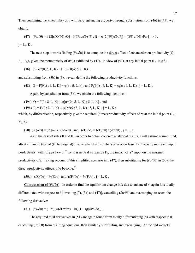
Then combining the k-neutrality of θ with its σ-enhancing property, through substitution from (46) in (45), we

obtain,

(47) (∂σ/∂θ) = σ{2[(∂Q/∂θ) /Q] � [(∂FLK/∂θ) /FLK]} = σ{2[(∂Fj/∂θ /Fj] � [(∂FLK/∂θ) /FLK]} > 0 ,

j = L, K .

The next step towards finding (∂k/∂σ) is to compute the direct effect of enhanced σ on productivity (Q,

FL , FK), given the monotonicity of σ*(.) exhibited by (47). In view of (47), at any initial point (Lo, Ko; δ),

(3b) σ = σ*(θ; δ, L, K) ⇔ θ = θ(σ; δ, L, K) ;

and substituting from (3b) in (1), we can define the following productivity functions:

(48) Q = F[θ(.) ; δ, L, K] ≡ φ(σ ; δ, L, k) ; and Fj[θ(.) ; δ, L, K] ≡ φj(σ ; δ, L, K) , j = L, K .

Again, by substitution from (3b), we obtain the following identities:

(49a) Q = F(θ ; δ, L, K) ≡ φ[σ*(θ ; δ, L, K) ; δ, L, K] , and

(49b) Fj = Fj(θ ; δ, L, K) ≡ φj[σ*(θ ; δ, L, K) ; δ, L, K] , j = L, K ;

which, by differentiation, respectively give the required (direct) productivity effects of σ, at the initial point (Lo,

Ko, δ):

(50) (∂Q/∂σ) = (∂Q/∂θ) / (∂σ/∂θ) , and (∂Fj/∂σ) = (∂Fj/∂θ) / (∂σ/∂θ) , j = L, K .

As in the case of rules II and III, in order to obtain concrete analytical results, I will assume a simplified,

albeit common, type of (technological) change whereby the enhanced σ is exclusively driven by increased input

porductivity, with (∂FLK/∂θ) = 0: 55 i.e. θ is neutral as regards Fij, the impact of ith input on the marginal

productivity of j. Taking account of this simplified scenario into (47), then substituting for (∂σ/∂θ) in (50), the

direct productivity effects of σ become,56

(50a) (∂Q/∂σ) = ½(Q/σ) and (∂Fj/∂σ) = ½(Fj/σ) , j = L, K .

Computation of (∂k/∂σ): In order to find the equilibrium change in k due to enhanced σ, again k is totally

differentiated with respect to θ [invoking (7), (3a) and (47)], cancelling (∂σ/∂θ) and rearranging, to reach the

following derivative:

(51) (∂k/∂σ) = (1/Y)[w(∂L*/∂σ) � kQ(1 � η)(∂P*/∂σ)] .

The required total derivatives in (51) are again found from totally differentiating (8) with respect to θ,

cancelling (∂σ/∂θ) from resulting equations, then similarly substituting and rearranging. At the end we get a

18

; 1 iff 0 e]} k) (1 [k / 1)] e)( ½{[(

ek) (1 [k / 1)] e)( ){[(½(L/ )/L( (52)

L

*

<>η

<>+η−+σ−η+σ=ε

⇔ ]} + η−+σ−η+σσ=σ∂∂

σ

. 0 e]} k) (1 [k / 1)] 1)( ]{[(/)k ½[k(1 )k/( )a51(<>+η−+σ−η−σσ−=σ∂∂

ly.respective , ) (or ) ( if ) (e or ) (e ]}k) (1 [k {e (54b)and ; 1 if )] ( [1 1) 1)( ( (54a)

such that , e] k) (1 e)[k (

e) 1)( 1)( ( ) k( Z, ] Z 2[e) k)( ½(1 Num )54( 112

1

σ<ησ>ηη+>σ+>η−+σ+>η+σση<η+σ−+ση=−η−σ

+η−+σ+η+σ−η−σ

ση−σ=−+η−=

. 2 Ziff 0 Num iff 0 )/( )55( 11 <>>σ∂λ∂

linear system identical to that in (29) except that δ is replaced by σ in the two columns.57 Substituting from

(50a) for (∂Fj/∂σ) and (∂Q/∂σ) in the RHS column, the required equilibrium derivatives can be found (by

Cramer�s rule) and rearranged into the following form:

where, εσj , j = L, P, is the σ-elasticity of j.

The total derivative of k is finally reached through substitution, from (52) and (53) in (51), and

rearranging:

Status of Rule I: Substituting from (51a) for (∂k/∂σ) in (22), its numerator can be reformulated as:

Evidently,from (22) and (54),

The determinate, Hicks/Bronfenbrenner formula obtains from (22) if Z1 = 0 : σ = 1 , η = 1 , or η = σ .

Yet the range of Z1 is comprised of the entire real line, and here, unlike rules II and III, the Hicks Qualification

is neither sufficient nor necessary for the validity of rule I because the sign and magnitude of Z1 hinge on the

tripartite expression (σ � η)(σ � 1)(η � 1) . However, it is useful to schematize the analysis into two scenarios,

depending on whether Hicks Qualification is effective.

(i) Hicks Qualification Scenario: Using (54a & b), Z1 in (54) can be decomposed into two terms (T1 +

T2, respectively) as follows:

(56a) Z1 = [kση(σ � η)(e + σ) / Den1] + [k(σ + η � 1)(η � σ)(e + σ) / Den1] , where

(56b) Den1 = σ(e + η)[e + kσ + (1 � k)η] > σ(e + η)(e + σ) > 0 , η > σ .

Because T1 < 0 , then Z1 < 2 if T2 ≤ 2 ; that is, if k(σ + η � 1) /σ ≤ 2, because, in view of (56b),

; 0 ]}k) (1 k [e / k)] (1 k ½{[e e]} k) (1 [k / k)] (1 k ){[e½(P/ )/P( )53(

P

*

<η−+σ+−+σ+−=ε⇔+η−+σ−+σ+σ−=σ∂∂

σ

19

. /e) 2( 1 if 0 )/( (60)

: (55) of in viewdrawn becan conclusion following theTherefore,

. ; e) (

e) (

e) ( e) (

e) ( ) k( Z)59(

2

2

2

221

η+η≤σ≤η<>σ∂λ∂

η≥σ+η

ησ<+η

+σση<+η

+σσησ

η−σ≤

(56c) T2 < [(η � σ) / (η + e)][k(σ + η �1) /σ] < k(σ + η � 1) /σ .

Therefore, by (55), the following conclusion can be reached:

(57) (∂λ/∂σ) > 0 if {σ < η ≤ [(2/k) � 1]σ + 1} .

It is noted that the preceding sufficient condition can be quite permissive not only because T1 is

negative but also because the fraction (η � σ) / (η + e) can become very small if e is large, or σ is close to η .

Alternatively, when Hicks Qualification is not in force (σ ≥ η), determining whether Z1 < 2 depends

critically on the sign configuration of (σ � 1)(η � 1), which gives rise to only three coherent (alternative)

variations to examine:

(ii) Only Technical Substitution Not Inelastic; σ ≥ η: In this case, because σ � η ≥ 0 and

(σ � 1)(η � 1) ≤ 0 , then, from (54), Z1 ≤ 0 < 2, and, in view of (55), we can conclude that,

(58) (∂λ/∂σ) > 0 if σ ≥ 1 ≥ η .

(iii) Both Substitution and Output Demand are Elastic; σ ≥ η: Hence, (σ � 1)(η � 1) > 1 , σ + η > 1 ,

and Z1 ≥ 0 such that Z1 < 2 if σ2 ≤ 2(η + e)2/η because, by (54), (54a) and (54b), we can infer that,

Again this condition can be quite permissive because of the succession of inequalities in (59) which lowers the

upper bound of σ in (60).

(iv) Both Substitution and Demand Not Elastic; σ ≥ η: In this case, because [1 > (σ � 1)(η � 1) ≥ 0] and

[1 > (σ � η) /σ ≥ 0] , we can deduce from (54) and (54b) that,

(61) Z1 ≤ (σ � 1)(η � 1)[(σ � η) /σ][k(σ + e) / (η + e)2] < [k(σ + e) / (η + e)2] .

Therefore, Z1 < 2 if [k(σ + e) / (η + e)2 ] ≤ 2 , and, again in view of (55), we conclude that,

(62) (∂λ/∂σ) > 0 if η ≤ σ ≤ [(2/k)(η + e)2 � e] and σ ≤ 1 .

Evidently, the upper bound of σ in (62) must have been curtailed in proportion to the fraction

[(σ � 1)(η � 1)(σ � η) /σ] in (61), among other factors.

The preceding analysis in (i) � (iv) is a proof of the following:

20

. 1 , e e) (2/k)( (iv) ; /e) 2( 1 (iii)

; 1 (ii) ; 1 1] [(2/k) )i(22 ≤σ−+η≤σ≤ηη+η≤σ≤η<

σ≤≤η+σ−≤η<σ

[ ] . 0) (1 iff 1 )/(lim ]k) (1 )[e (e

1) ke( Z)c54(0 1 >η>∞−→−ση

���

���

η−+η+−η=

→σ

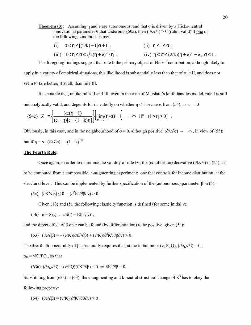
Theorem (3): Assuming η and e are autonomous, and that σ is driven by a Hicks-neutral innovational parameter θ that underpins (50a), then (∂λ/∂σ) > 0 (rule I valid) if one of the following conditions is met:

The foregoing findings suggest that rule I, the primary object of Hicks� contribution, although likely to

apply in a variety of empirical situations, this likelihood is substantially less than that of rule II, and does not

seem to fare better, if at all, than rule III.

It is notable that, unlike rules II and III, even in the case of Marshall�s knife-handles model, rule I is still

not analytically valid, and depends for its validity on whether η < 1 because, from (54), as σ → 0

Obviously, in this case, and in the neighbourhood of σ = 0, although positive, (∂λ/∂σ) → + ∞ , in view of (55);

but if η = σ , (∂λÚ∂σ) → (1 � k).58

The Fourth Rule:

Once again, in order to determine the validity of rule IV, the (equilibrium) derivative (∂k/∂e) in (25) has

to be computed from a compossible, e-augmenting experiment: one that controls for income distribution, at the

structural level. This can be implemented by further specification of the (autonomous) parameter β in (5):

(5a) (∂Ks/∂β) ≤ 0 , (∂2Ks/∂β∂v) > 0 .

Given (13) and (5), the following elasticity function is defined (for some initial v):

(5b) e = S′(.) . v/S(.) = E(β ; v) ;

and the direct effect of β on e can be found (by differentiation) to be positive, given (5a):

(63) (∂e/∂β) = � (e/K)(∂Ks/∂β) + (v/K)(∂2Ks/∂β∂v) > 0 .

The distribution neutrality of β structurally requires that, at the initial point (v, P, Q), (∂αK/∂β) = 0 ,

αK = vKs/PQ , so that

(63a) (∂αK/∂β) = (v/PQ)(∂Ks/∂β) = 0 � ∂Ks/∂β = 0 .

Substituting from (63a) in (63), the e-augmenting and k-neutral structural change of Ks has to obey the

following property:

(64) (∂e/∂β) = (v/K)(∂2Ks/∂β∂v) > 0 .

21

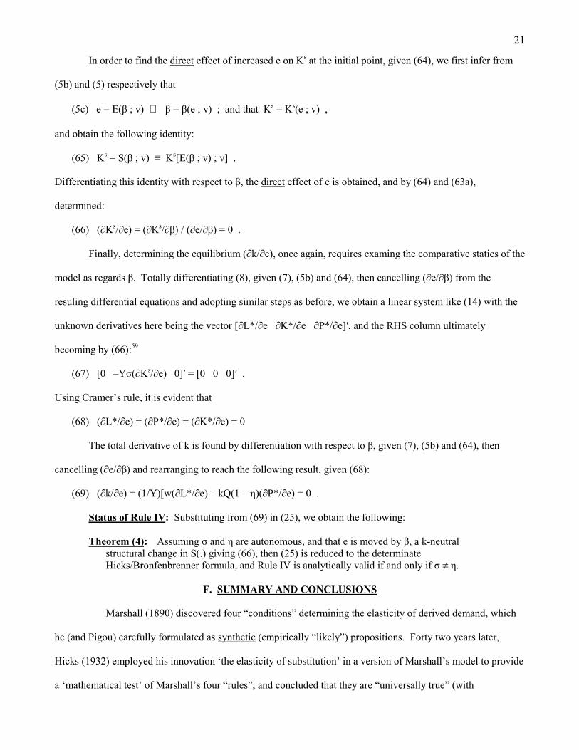
In order to find the direct effect of increased e on Ks at the initial point, given (64), we first infer from

(5b) and (5) respectively that

(5c) e = E(β ; v) ⇔ β = β(e ; v) ; and that Ks = Ks(e ; v) ,

and obtain the following identity:

(65) Ks = S(β ; v) ≡ Ks[E(β ; v) ; v] .

Differentiating this identity with respect to β, the direct effect of e is obtained, and by (64) and (63a),

determined:

(66) (∂Ks/∂e) = (∂Ks/∂β) / (∂e/∂β) = 0 .

Finally, determining the equilibrium (∂k/∂e), once again, requires examing the comparative statics of the

model as regards β. Totally differentiating (8), given (7), (5b) and (64), then cancelling (∂e/∂β) from the

resuling differential equations and adopting similar steps as before, we obtain a linear system like (14) with the

unknown derivatives here being the vector [∂L*/∂e ∂K*/∂e ∂P*/∂e]′, and the RHS column ultimately

becoming by (66):59

(67) [0 �Yσ(∂Ks/∂e) 0]′ = [0 0 0]′ .

Using Cramer�s rule, it is evident that

(68) (∂L*/∂e) = (∂P*/∂e) = (∂K*/∂e) = 0

The total derivative of k is found by differentiation with respect to β, given (7), (5b) and (64), then

cancelling (∂e/∂β) and rearranging to reach the following result, given (68):

(69) (∂k/∂e) = (1/Y)[w(∂L*/∂e) � kQ(1 � η)(∂P*/∂e) = 0 .

Status of Rule IV: Substituting from (69) in (25), we obtain the following:

Theorem (4): Assuming σ and η are autonomous, and that e is moved by β, a k-neutral structural change in S(.) giving (66), then (25) is reduced to the determinate Hicks/Bronfenbrenner formula, and Rule IV is analytically valid if and only if σ ≠ η.

F. SUMMARY AND CONCLUSIONS

Marshall (1890) discovered four �conditions� determining the elasticity of derived demand, which

he (and Pigou) carefully formulated as synthetic (empirically �likely�) propositions. Forty two years later,

Hicks (1932) employed his innovation �the elasticity of substitution� in a version of Marshall�s model to provide

a �mathematical test� of Marshall�s four �rules�, and concluded that they are �universally true� (with

22

only a minor Qualification to the third rule). And apart from a sporadic dispute about Hicks Qualification,

which was resolved by Maurice (1975), the Hicksian �testing method� has been uncritically accepted by

researchers, and his conclusions have been generally viewed as analytical (�universal�) laws in both textbooks

and empirical work, to date.

The primary aim of this study has been twofold: First, formulating a model that captures the salient

features of Hicks� Marshallian model, and employing it to demonstrate: 1) that none of Hicks� rules is

analytically determinate (let alone �universally true�), an indeterminancy that can be explained by invoking the

�Allen-type� decomposition; and 2) that his �universality� claim is a consequence of a flawed testing method,

implicitly involving improper assumptions (notably that k is fixed). Second, developing a �testing� method

rooted in Marshallian comparative statics, and deploying it in producing �likely� sets of sufficient conditions for

the validity of Marshall�s laws.

The four sets of sufficient conditions I obtained are summarized in theorems (1) to (4). Being a

consequence of the �experimental design� described above (and its stated assumptions), these conditions merit

the following remarks:

First, assuming the autonomousness of σ, η and e, Hicks� Qualification (η > σ) remains a necessary

and sufficient condition for the validity of Marshall�s third law. Ironically, the only controversial (until 1975)

Hicksian finding, turned out to be the least problematic among his conclusions regarding Marshall�s laws.

Second, besides the autonomousness of σ and e, Hicks� Qualification is also a sufficient condition for the

validity of rule II. The alternative sets of conditions developed above suggest that � by and large � substantially

less stringent conditions (than those of rule III) are sufficient for rule II.

Third, in contrast to rules II and III, Hicks Qualification is neither necessary nor sufficient for the

validity of rule I. Moreover, the alternative sets of sufficient conditions in theorem (3) are substantially more

restrictive than those of rule II and � to a lesser extent � rule III. This finding is particularly interesting, not only

because rule I is the only one for which Marshall�s Principles had not reported a demonstration, but also

because this demonstration was the primary object of Hicks� mathematical investigation.

Fourth, if σ and η are autonomous, we obtain the Hicksian result that Marshall�s fourth law is

analytically valid, albeit with the minor qualification that σ ≠ η. As such, this one, being the least invoked (of

23

the four laws) in textbooks and empirical work on derived demand, stands in sharp contrast to the most invoked

law, the first rule, whose sufficient conditions are found to be the most restrictive of all.60 Fifth, we also found

that with Marshall�s knife-handles model (and same experimental design), like IV, rules II and III become also

unequivocally valid, but � interestingly again � rule I continues to be indeterminate. It becomes valid, however,

if η < 1, and (∂λÚ∂σ) finite if η = σ .

Sixth, at the risk of being repetitive, it is important to emphasize that the preceding conclusions (and

their underlying analysis) are all about the logical validity � not universal truth � of Marshall�s �laws�. For the

Marshallian �laws� to be true � besides their logical validity � all their premises must be �true�: that is, all their

conditions and assumptions (including constant returns to scale, perfect competition, profit maximization, etc.)

must be true.61 The accumulating econometric evidence [surveyed in Hamermesh (1993)] provides a

compelling empirical basis in this regard (at least for labour demand).62 As such, it lends substantial support for

the plausibility of Marshall�s �laws� as being the �synthetic�, �empirical generalizations� Marshall, the great

British Empiricist of neoclassicism, intended them to be � I think63 � and this stands in sharp contrast to the

epistemological predilection of the author of The Theory of Wages.64 The preceding remarks also suggest that

this (empirical) plausibility varies: it progressively increases from the first law, to the third, then the second,

and reaches a climax in the fourth.

Finally, it is tempting to conclude that the preceding conclusions and underlying analysis may

constitute an explanation for the nuanced and qualified (by �likely�) formulation of the laws of derived demand

as originally cast by Marshall (and Pigou). And in this capacity, this study may lend additional support to the

belief � maintained by Hicks (1932: pp. 241 f) � that �marshall himself no doubt derived his rules from

Mathematics�,65 and � I should add � correctly at that. And yet, despite the strong evidence, this conclusion

cannot be archivally verified by this author and � alas � will have to remain in the realm of conjecture �

however compelling � as an open research question in the history of economic ideas and method. But if the

thesis advanced by this study is correct, the great Empiricist cofounder of Neoclassicism, the meticulous

promulgator of the laws of derived demand (towards the end of the nineteenth century), should be smiling �

hopefully not at us � from his ethereal vantage, on the eve of the twenty-first century.

24

ENDNOTES

1 Historians of thought argue about whether Marshall is �the father� of neoclassical economics, as Landreth and Colander(1994: pp. 285 f) put it. Others such as Ekelund and Hébert (1990) credit Walras with an equal contribution. Sincemodern neoclassicism descends from a marriage between the Continental Rationalist tradition that emphasizes systems(Walras) and British Empiricism that emphasizes the �parts� (Marshall), perhaps it is best to consider Marshall and Walrasas its �lawful parents�, and relegate their proverbial rivalry into a mere �dispute over custody�. Marshall (1890: p.v)himself thought of his �treatise� as being �an attempt to present a modern version of old doctrines with the aid of the newwork, and with reference to the new problems of our own age�. He modelled his method and work �in accordance withEnglish [Empiricist] traditions�, which was articulated by David Hume, elaborated and applied (in economics) by AdamSmith and J.S. Mill; on Marshall�s method and its geneology, see Bk. I and Appendices B, C and D. All Marshall pagereferences are to the English-Language-Book-Society edition (1969) of 8th edition. On these competing philosophicaltraditions in general, see Copleston (1985), especially Vols. IV-VI and VIII, and in economics, see Jaffé (1977) andPokornỳ (1978).2 Illustrating by �one class of labour�, �the plasterers�, Marshall (1920: p. 320) generalizes: �The relations betweenplasterers, bricklayers, etc., are representative of much that is both instructive and romantic in the history of alliances andconflicts between trade-unions in allied trades�.3 In characterizing the logical progression of applying his partial-equilibrium method, in the preface to the 8th edition (nearthe sunset of his long life) Marshall (1920: p. xiii) states that �the area covered by provisional statical assumptionsbecomes smaller; and at last is reached the great central problem of the Distribution of the National Dividend�. And, in hisintroductory chapter, Marshall (pp. 1f) expounds his doctrinal view that �The question whether poverty is necessary givesits highest interest to economics�. For a review of his socioeconomic doctrine, see Pigou (1953), Ch. 6 and Whitaker(1987: pp. 352-53).4 On his mathematical gifts, experience and method, see Pigou (1953), Ch. I, Whitaker (1987: pp. 350-51), and Landrethand Colander (1994: pp. 285-92).5 Pigou�s statement is rearranged to conform with Marshall�s original numbering of the conditions. There are subtledifferences between this and Marshall�s own formulation of the conditions which may prove significant to theirdemonstration; but Pigou�s is the statement quoted in Hicks (1932).6 He did not demonstrate condition I mathematically or graphically. Conditions II-IV were only stated mathematically; andreferring to these, Marshall stated that � in the case of variable production coefficients � a �more complex inquiry, leads tosubstantially the same results� (p. 702: emphasis added).7 The term �puzzle� is used relative to what Kuhn considers to be part of the conduct of �normal science� under the bannerof a victorious paradigm, viz. neoclassicism. See Kuhn (1970), chs. 3, 4.8 This is similar to the question Pigou (1924, 1932) investigated in part IV, chs. 4-5.9 The term �coefficients of production� is due to Walras who, like Marshall, assumed its variability; Hicks (1932: p. 117 n)related it to his elasticity of substitution. On this issue, see Stigler (1939) and note (11) below.10 Joan Robinson also developed the same concept, independently. See Helm (1987).11 Marshall introduced technical substitution through {mj}, a set of variable input coefficients, in the output supply equationof note XIV model. Hicks (1920: p. 237), unlike Marshall and Pigou, introduced a separate production function noting that�it is naturally given by technical considerations�, �once we grant the universality of substitution�. Curiously the term�production function� does not appear in Hicks (1939) Value and Capital.12 Like technical substitution, this aspect of production technology was not new, and was discussed in terms of whatJohnson (1913) called �the elasticity of production�; see Ferguson (1971: pp. 79 f). But research on this aspect ofproduction functions (both theoretical and empirical) escalated after Cobb and Douglas (1928) contribution.13 In the first edition, Hicks (1932) adopted a different rule-numbering than Marshall�s, but reverted to the latter in Hicks(1961) upon a suggestive remark by Bronfenbrenner (1961).14 Pigou�s previously stated formulation, which was used by Hicks (1932), captured the spirit of Marshall�s in this regard:Marshall qualified his conditions by a �may�. The terms �analytic� and �synthetic� are used in the sense given to them inKantian logic. Strictly speaking, Hicks seems to be confusing �logical validity� with the �universal truth� of propositions.Besides �validity�, universal �truth� requires that his �premises� (notably the assumptions of constant returns to scale, perfectcompetition and profit maximization) be (empirically) �true�.15 Shove, however, noted that �The rigid assumptions . . . made [by Hicks, e.g. constant returns to scale] deprive thetheoretical conclusions of generality . . . .� To the best of my knowledge this subtle change in the status of Marshall�s lawshas not been given due attention by anyone as yet.

25

16 Allen did not, however, �test� Marshall�s laws (by partial differentiation) like Hicks. Using a similar model, but with theprices of cooperant inputs exogenous, Allen (1938: pp. 369-74, 502-9) produced Marshall/Hicks formulas of price (ownand cross) elasticities for both the two- and multi-input cases. Allen also analyzed his formulas in terms of the output(scale) and substitution effects à la Slutsky, based on Allen and Hicks (1934).17 With the above-mentioned work of Allen (1938), and Mosak (1938), research work shifted to investigating the sensitivityanalysis of input demand in terms of the �fundamental equation of value theory�.18 The appellation �laws� goes back at least to Bronfenbrenner (1961).19 Bronfenbrenner (1961: p. 259), however, misinterpreted Allen�s model stating that �Allen developed a model ofindividual demand by a single competitive entrepreneur� [my emphasis]. In fact, Allen (1938: pp. 372 f) never said that,and in his elasticity formulas (which includes the elasticity of output demand) he explicitly assumed output price to beendogenous, but that the product �is sold on a competitive market at a price P . . .�20 He also recognized that the Marshall and Allen formulas are special cases of Hicks� when σ→0 and e→∞, respectively.21 Bronfenbrenner (1961: pp. 258 f) attempted unsuccessfully.22 In fact Hicks� �literary demonstration� is not so convincing because his argument (on p. 264) implicitly assumes thatλ < 1, and he also utilizes an extra-model, but supposedly �intelligible�, argument to explain the �paradox�.23 Other studies include Saving (1963), Munlak (1968), Diewert (1971), Sakai (1973) and Wisecarver (1974).24 Although he did not test Marshall�s laws, Muth (1964: p. 228) employed Hicks� method of �partial differentiation� togenerate analogous laws for output supply, and found that supply elasticity �is greater the greater the relative importance ofthe factor whose supply is the more elastic�.25 Other contributions on input demand include Ferguson (1966), Ferguson (1967) and Ferguson (1968), but much of thiswork was incorporated in Ferguson (1971).26 Diewert (1971) also derived an elasticity formula of the multi-input case, but did not attempt testing Marshall laws,stating only that his formula �could be used to compute numerically how the elasticity of derived demand . . . varies withrespect to admissible changes in the other elasticities� (p. 198).27 Maurice (1975: pp. 391 f) also demonstrated that the Bronfenbrenner (1971) �blind alley� claim was �in error because ofinternal contradictions�. On the direction research on input demand has taken in the area of labour, see Freeman (1987) andHamermesh (1993).28 This is especially true of the first three laws. Thus, Allen�s elasticity formula, which assumes an exogenous v, is heavilyused in empirical research as the recent survey by Hamermash (1993) indicates. Upon surveying a large number oftextbooks, I found that: First, the first three laws are typically stated in introductory and intermediate micro bookswhenever input demand is discussed, but mostly without reference to Marshall or to Hicks� qualification. Second, the lawsare rarely discussed in advanced micro textbooks: the latest systematic exposition was Layard and Walters (1978), andonly Gravelle and Rees (1992) and Nicholson (1998) derive Allen�s formula, but without �testing� the laws. Taken as one,the two findings are a measure of the �universal� acceptance of Marshall�s laws to the extent of becoming commonplace.29 The model is contained in Ch. VI and laid out in the Appendix. Subsequent contributions by Hicks did not introduce anysubstantive change to the model. These include Hicks (1935), Hicks (1936) and Hicks (1961) which were included in thesecond edition of the book, Hicks (1963); the latter also contained a �Commentary� on the first edition.30 In the interest of generality, Hicks presented his appendix model in terms of inputs a and b, but in the text of ch. VI (p.119) he dealt with labour and capital following Pigou, who categorized factors of production into labour and capital(�supposing that land can be neglected�) in his own investigation on income distribution.31 Usually represented in growth models by one parameter, it is appropriate for our purpose to think in terms of two distincttypes of technological change, represented by separate parameters, both �autonomous� à la Hicks. Agreeing with Pigouthat �inventions have a decided bias in the labour-saving direction, Hicks (1932 f.) classified inventions into �autonomous�and �induced�; only the latter is determined by relative input prices.32 In his decomposition, however, Allen (1938) assumed v exogenous as indicated above, and in his analysis Hicks (1961)employed the results of Allen�s special case. It is notable that the output effect is the same for both L and K because oftheir unitary output-elasticites, in view of the linear homogeneity of F(.).33 Similarly, in the case of σ because his distinction between �induced� and �autonomous� inventions was part of a longdiscussion on the determinants of σ (pp. 120-130). Following Hicks, Muth (1964), Bronfenbrenner (1961, 1971), Sato andKoizumi (1970), Ferguson (1971), and Maurice (1972) adopted the same practice, although only the last author recognizedits problematic nature in Maurice (1975) as he addressed the third-rule paradox.34 Hicks (1932: p. 233) states that �the chief value of such a Mathematical proof must lie in the disclosure of the exactassumptions and the precise limitations under which the propositions are true�. Yet, nowhere did he disclose that σ, η or eare autonomous parameters. On the contrary, his model and those of others make it clear that they are endogenous. OnlySato and Koizumi (1970: p. 112) assumed them �fixed� and only at the stage of testing the rules (by partial differentiation);they also extended this assumption to include their factor shares{αi}.

26

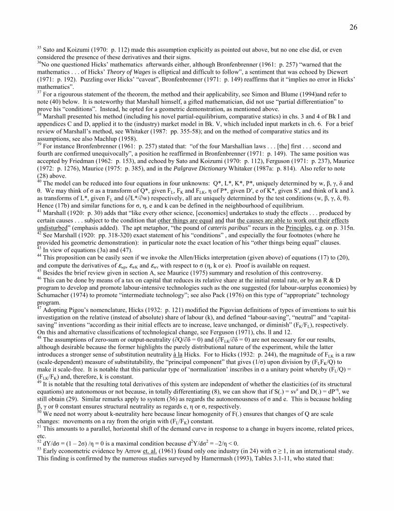
35 Sato and Koizumi (1970: p. 112) made this assumption explicitly as pointed out above, but no one else did, or evenconsidered the presence of these derivatives and their signs.36No one questioned Hicks� mathematics afterwards either, although Bronfenbrenner (1961: p. 257) �warned that themathematics . . . of Hicks� Theory of Wages is elliptical and difficult to follow�, a sentiment that was echoed by Diewert(1971: p. 192). Puzzling over Hicks� �caveat�, Bronfenbrenner (1971: p. 149) reaffirms that it �implies no error in Hicks�mathematics�.37 For a rigourous statement of the theorem, the method and their applicability, see Simon and Blume (1994)and refer tonote (40) below. It is noteworthy that Marshall himself, a gifted mathematician, did not use �partial differentiation� toprove his �conditions�. Instead, he opted for a geometric demonstration, as mentioned above.38 Marshall presented his method (including his novel partial-equilibrium, comparative statics) in chs. 3 and 4 of Bk I andappendices C and D, applied it to the (industry) market model in Bk. V, which included input markets in ch. 6. For a briefreview of Marshall�s method, see Whitaker (1987: pp. 355-58); and on the method of comparative statics and itsassumptions, see also Machlup (1958).39 For instance Bronfenbrenner (1961: p. 257) stated that: �of the four Marshallian laws . . . [the] first . . . second andfourth are confirmed unequivocally�, a position he reaffirmed in Bronfenbrenner (1971: p. 149). The same position wasaccepted by Friedman (1962: p. 153), and echoed by Sato and Koizumi (1970: p. 112), Ferguson (1971: p. 237), Maurice(1972: p. 1276), Maurice (1975: p. 385), and in the Palgrave Dictionary Whitaker (1987a: p. 814). Also refer to note(28) above.40 The model can be reduced into four equations in four unknowns: Q*, L*, K*, P*, uniquely determined by w, β, γ, δ andθ. We may think of σ as a transform of Q*, given FL, FK and FLK, η of P*, given D′, e of K*, given S′, and think of k and λas transforms of L*, given FL and (∂L*/∂w) respectively, all are uniquely determined by the test conditions (w, β, γ, δ, θ).Hence (17b) and similar functions for σ, η, e and k can be defined in the neighbourhood of equilibrium.41 Marshall (1920: p. 30) adds that �like every other science, [economics] undertakes to study the effects . . . produced bycertain causes . . . subject to the condition that other things are equal and that the causes are able to work out their effectsundisturbed� (emphasis added). The apt metaphor, �the pound of cæteris paribus� recurs in the Principles, e.g. on p. 315n.42 See Marshall (1920: pp. 318-320) exact statement of his �conditions� , and especially the four footnotes (where heprovided his geometric demonstration): in particular note the exact location of his �other things being equal� clauses.43 In view of equations (3a) and (47).44 This proposition can be easily seen if we invoke the Allen/Hicks interpretation (given above) of equations (17) to (20),and compute the derivatives of εwp, εwK and εwv with respect to σ (η, k or e). Proof is available on request.45 Besides the brief review given in section A, see Maurice (1975) summary and resolution of this controversy.46 This can be done by means of a tax on capital that reduces its relative share at the initial rental rate, or by an R & Dprogram to develop and promote labour-intensive technologies such as the one suggested (for labour-surplus economies) bySchumacher (1974) to promote �intermediate technology�; see also Pack (1976) on this type of �appropriate� technologyprogram.47 Adopting Pigou�s nomenclature, Hicks (1932: p. 121) modified the Pigovian definitions of types of inventions to suit hisinvestigation on the relative (instead of absolute) share of labour (k), and defined �labour-saving�, �neutral� and �capital-saving� inventions �according as their initial effects are to increase, leave unchanged, or diminish� (FK/FL), respectively.On this and alternative classifications of technological change, see Ferguson (1971), chs. ll and 12.48 The assumptions of zero-sum or output-neutrality (∂Q/∂δ = 0) and (∂FLK/∂δ = 0) are not necessary for our results,although desirable because the former highlights the purely distributional nature of the experiment, while the latterintroduces a stronger sense of substitution neutrality à la Hicks. For to Hicks (1932: p. 244), the magnitude of FLK is a raw(scale-dependent) measure of substitutability, the �principal component� that gives (1/σ) upon division by (FLFK/Q) tomake it scale-free. It is notable that this particular type of �normalization� inscribes in σ a unitary point whereby (FL/Q) =(FLK/FK) and, therefore, k is constant.49 It is notable that the resulting total derivatives of this system are independent of whether the elasticities (of its structuralequations) are autonomous or not because, in totally differentiating (8), we can show that if S(.) = sve and D(.) = dP-η, westill obtain (29). Similar remarks apply to system (36) as regards the autonomousness of σ and e. This is because holdingβ, γ or θ constant ensures structural neutrality as regards e, η or σ, respectively.50 We need not worry about k-neutrality here because linear homogenity of F(.) ensures that changes of Q are scalechanges: movements on a ray from the origin with (FL/FK) constant.51 This amounts to a parallel, horizontal shift of the demand curve in response to a change in buyers income, related prices,etc.52 dY/dσ = (1 � 2σ) /η = 0 is a maximal condition because d2Y/dσ2 = �2/η < 0.53 Early econometric evidence by Arrow et. al. (1961) found only one industry (in 24) with σ ≥ 1, in an international study.This finding is confirmed by the numerous studies surveyed by Hamermash (1993), Tables 3.1-11, who stated that:

27

�examining estimates based on microeconomic data does not alter the conclusion reached from aggregate data . . ., themean estimate of σ is somewhat lower, 0.49, [than 0.75, the mean estimate from aggregate data]� (pp. 103, 92).54 It can be easily shown that (∂k/∂θ) = LK(FK/Q)2[∂(FL/FK) / ∂θ].55 This assumption, which is not necessary for our general results, represents a stronger sense of neutrality as regardsrelative input porductivities because (∂FLK/∂θ) = ∂(∂FL/∂K) /∂θ, and because it implies that (∂FLL/∂θ) = (∂FKK/∂θ) = 0, inview of (2). This amounts to saying that θ does not affect the severity of the law of variable proportions.56 This result stems from the input-saving nature of θ: hence, given L and K, an increase in σ causes Q, FL and FK toincrease to the same extent in view of input neutrality.57 Again, the resulting total derivatives here are independent of whether η and e are autonomous, for the same reasons as innote (49).58 Evidently, Z1 → 0 if η = σ, by (54c); and (22) then gives (∂λ/∂σ) = ( 1 � k) > 0.59 The total derivatives of this system are also independent of whether η and σ are autonomous for reasons explained in note(49).60 Refer to note (28) above.61 Refer to notes (14) and (15) above.62 Refer to note (53) above.63 Refer to note (1) on Marshall�s empiricist orientation, and his incisive comment in note (2) which was occasioned by hischaracteristic zeal to illustrate the explanatory power of his laws by a variety of empirical instances.64 Reminiscing on his intellectual orientation at the time of writing the book, Hicks (1963: p. 306) states that �with all ofwhom [notably Walras] I was much more at home . . . than I was with Marshall and Pigou. (We were such �goodEuropeans� in London that it was Cambridge that seemed �foreign�.)�.65Hicks adds: �But he does not there give the full mathematical derivation; he confines himself to a simplified case . . . .�Marshall (1920: p. ix) himself states that only �A few specimens of those applications of mathematical language whichhave proved most useful for my own purposes have, however, been added in an Appendix�. Refer also to notes (4) and (6)above.

28

REFERENCES

Allen, R.G.D. (1938) Mathematical Analysis for Economists (London: Macmillan).

Arrow, K.J., Chenery, H.B., Minhas, B. and Solow, R.M. (1961) “Capital-Labour Substitution and EconomicEfficiency”, Review of Economics and Statistics, vol. 43, pp. 225-50.

Bronfenbrenner, M. (1961) “Notes on the Elasticity of Derived Demand”, Oxford Economic Papers, vol. 13, pp.254-61.

_____ (1971) Income Distribution Theory, (London: MacMillan), ch. 6.

Copleston, S.J., F. (1985) A History of Philosophy, books Two and Three, (New York: Image Books, Doubleday).

Cobb, C.W. and Douglas, P.H. (1928) “A Theory of Production”, American Economic Review, vol. 18, no. 1,suppl. pp. 139-65.

Diewert, W.E. (1971) “A Note on the Elasticity of Derived Demand in the n-factor Case.” Economica, vol. 38, pp.192-98.

Eatwell, J. et. al., editors (1987) The New Palgrave Dictionary of Economics (London: Macmillan).

Ekelund, JR., R.B. and Hébert, R.F. (1990) A History of Economic Theory and Method, 3rd edition (New York:McGraw-Hill).

Ferguson, C.E. (1966) “Production, Prices, and the Theory of Jointly-Dervied Input Demand Functions”,Economica, vol. 33, pp. 454-61.

_____ (1967) “The Theory of Input Demand and the Role of ‘Inferior factors’ in the Theory of Production”, Revued’Economie Politique, vol. 77, pp. 413-33.

_____ (1968) “‘Inferior Factors’ and the Theories of Production and Input Demand”, Economica, vol. 35, pp. 140-50.

_____ (1971) The Neoclassical Theory of Production and Distribution (Cambridge: Cambridge Univ. Press), ch.12.

Freeman, R.B. (1987) “Labour Economics”, Eatwell et. al. eds. (1987), New Palgrave, vol. 3, pp. 73-6.

Friedman, M. (1962) Price Theory: A Provisional Text (Chicago: Aldine), ch. 7.

Gravelle, H. and Rees, R. (1992) Microeconomics 2nd edition (London: Longman) ch. 14.

Hamermesh, D.S. (1993) Labor Demand (Princeton: Princeton University Press).

Helm, D.R. (1987) “Elasticity of Substitution”, Eatwell et. al. eds. (1987), New Palgrave, vol. 2, pp. 127-28)

Henderson, D.H. (1921) Supply and Demand. (Chicago: Nisbet and University of Chicago Press, 1963).

Hicks, J.R. and Allen, R.G.D. (1934) “Reconsideration of the Theory of Value”, Part I and II, Economica, vol. 1,pp. 52-75, 196-219.

29

Hicks, J.R. (1935) “Wages and Interest: The Dynamic Problem”, The Economic Journal, reprinted in Hicks(1963), pp. 268-85.

_____ (1936) “Distribution and Economic Progress: A Revised Version”, Review of Economic Studies, vol. 4,reprinted in Hicks (1963), pp. 286-303.

_____ (1939) Value and Capital (Oxford: Clarendon Press; second edition, 1946).

_____ (1961) “Marshall’s Third Rule: A Further Comment”, Oxford Economic Papers, vol. 13, pp. 262-65.

_____ (1932) Theory of Wages (London: Macmillan; 2nd edition, 1963).

Jaffé, W. (1977) “A Centenarian on a Bicentenarian: Léon Walras’ Elements, on Adam Smith’s Wealth ofNations”, Canadian Journal of Economics, vol. 10, no. 1, pp. 19-33.

Kuhn, T.S. (1970) The Structure of Scientific Revolutions, 2nd edition (Chicago: University of Chicago Press).

Landreth, H. and Colander, D.C. (1994) History of Economic Thought, 3rd edition (Boston: Houghton Mifflin).

Layard, P.R.G. and Walters, A.A. (1978) Microeconomic Theory (New York: McGraw-Hill), ch. 9.

Machlup, F. (1958) “Equilibrium and Disequilibrium: Misplaced Concreteness and Disguised Politics”, TheEconomic Journal, vol. 68, pp. 1-24.

Marshall, A. (1890, 1920) Principles of Economics, 8th edition (London: English Language Book Society andMacmillan, 1969).

Maurice, S.C. (1972) “Long-run Factor Demand in a Perfectly Competitive Industry”, Journal of PoliticalEconomy, vol. 80, pp. 1271-79.

_____ (1975) “On the Importance of Being Unimportant: An Analysis of the Paradox in Marshall’s Third Rule ofDerived Demand”, Economica, vol. 42, pp. 385-93.

Mosak, J.L. (1938) “Interrelations of Production, Price and Derived Demand”, Journal of Political Economy, vol.46, pp. 761-87.

Mundlak, Y. (1968) “Elasticities of Substitution and the Theory of Derived Demand”, Review of EconomicStudies, vol. 35, pp. 225-36.

Muth, R.F. (1964) “The Derived Demand Curve for a Productive Factor and the Industry Supply Curve”, vol. 16,Oxford Economic Papers, pp. 221-34.

Nicholson, W. (1998) Microeconomic Theory: Basic Principles and Extensions, 7th edition (Fort Worth Tx: TheDryden Press), ch. 21.

Pack, H. (1976) “Policies to Encourage the Use of Intermediate Technology”, Development Digest, vol 14, no. 4,pp. 94-108.

Pigou, A.C. (1924, 1932) Economics of Welfare, 2nd and 4th edition (London: MacMillan).

_____ (1953) Alfred Marshall and Current Thought (London: MacMillan).

30

Pokorný, D. (1978) “Smith and Walras: Two Theories of Science”, Canadian Journal of Economics, vol 11, no. 3,pp. 387-403.

Sakai, Y. (1973) “An Axiomatic Approach to Input Demand Theory”, International Economic Review, vol. 14, no.3, pp. 735-52.

Sato, R. and Koizumi, T. (1970) “Substitutability, Complementarity and the Theory of Derived Demand”, Reviewof Economic Studies, vol 37, pp. 107-18.

Saving, T.R. (1963) “Note on Factor Demand Elasticity: The Competitive Case”, Econometrica, vol 31, pp. 555-57.

Schumacher, E.F. (1974) Small is Beautiful: A Study of Economics as if People Mattered (London: ABACUS).

Shove, G.F. (1933) “Review of ‘The Theory of Wages’”, The Economic Journal, reprinted in Hicks (1963), pp.249-67.

Simon, C.P. and Blume, L. (1994) Mathematics for Economists (New York: W.W. Norton).

Stigler, G. (1939) “Production and Distribution in the Short Run”, Journal of Political Economy, reprinted in AEA,Readings in the Theory of Income Distribution, London, George Allen & Unwin Ltd., pp. 119-42.

Whitaker, J.K. (1987) “Marshall, Alfred”, Eatwell et. al. eds., (1987), New Palgrave, vol. 3, pp. 350-63.

_____ (1987a) “Derived Demand”, in Eatwell et. al. eds. (1987), New Palgrave, vol. 1, pp. 313-14.

Wisecarver, D. (1974) “The Social Costs of Input-market Distortions”, American Economic Review, vol. 64, pp.359-72.