widening participation in higher education: analysis … · widening participation in higher...
TRANSCRIPT

Widening Participation in Higher Education: Analysis using Linked Administrative Data
Haroon Chowdry Institute for Fiscal Studies
Claire Crawford Institute for Fiscal Studies
Lorraine Dearden Institute for Fiscal Studies; Institute of Education, University of London
Alissa Goodman Institute for Fiscal Studies
Anna Vignoles Institute of Education, University of London
Copy-edited by Judith Payne
The Institute for Fiscal Studies 7 Ridgmount Street London WC1E 7AE

Published by The Institute for Fiscal Studies
7 Ridgmount Street London WC1E 7AE
tel. +44 (0) 20 7291 4800 fax +44 (0) 20 7323 4780 email: [email protected]
http://www.ifs.org.uk
© The Institute for Fiscal Studies, July 2008 ISBN: 978-1-903274-55-2

Preface
We are grateful for funding from the Economic and Social Research Council (grant number RES-139-25-0234) via its Teaching and Learning Research Programme (TLRP). In addition, we would like to thank the Department for Children, Schools and Families – Anna Barker, Graham Knox and Ian Mitchell in particular – for facilitating access to the valuable data-set we have used. Without their work on linking the data and facilitating our access, this work could never have come to fruition. We are also grateful for comments from Stijn Broecke, Joe Hamed and John Micklewright and from participants at various seminars and conferences, particularly the British Education Research Association Annual Conference and those organised by TLRP. Responsibility for interpretation of the data, as well as for any errors, is the authors’ alone.

Contents Executive summary i 1. Background and motivation 1 1.1 Introduction 1 1.2 Background 2 1.3 Previous research 4 2. Data 6 2.1 The data-sets that we use 6 2.2 Control variables 9 2.3 Sample selection 11 3. Sample description 12 3.1 Who participates in higher education? 12 3.2 Which types of universities do they attend? 17 3.3 Which subjects do they study? 22 4. Methodology 28 5. Participation in higher education 31 5.1 Baseline estimates of differences in HE participation rates 31 5.2 The importance of prior attainment 38 5.3 Changes in attainment over time and HE participation rates 42 5.4 Conclusions 50 6. Status of HE institution attended 52 6.1 Baseline estimates of differences in status of HE institution attended 52 6.2 The role of prior attainment in the HE status gradient 59 6.3 Conclusions 64 7. Subject choice 65 7.1 STEM subjects 65 7.2 Law 73 7.3 Subject studied, by wage return 81 7.4 Conclusions 85 8. Conclusions 87 Appendix A. More descriptive statistics 90 Appendix B. Characteristics of HE participants who study Maths or 94 Medicine Appendix C. Comparison of HE participants across years 98 Appendix D. Gradients associated with studying Maths at university 100 Appendix E. Gradients associated with studying Medicine at university 108 References 114
i
Executive Summary
Higher education (HE) participation has expanded dramatically in England over the last half century. Yet although participation has been rising, ‘widening participation’ in HE remains a major policy issue. Of particular concern is whether expansion of HE has led to improvements in the representation of previously under-represented groups, such as students from lower socio-economic backgrounds and ethnic minority students.
This study has been motivated by empirical evidence that suggests that the gap in the HE participation rate between richer and poorer students actually widened in the mid- and late 1990s (Blanden and Machin, 2004; Machin and Vignoles, 2004; HEFCE, 2005), although this trend has since reversed somewhat (Raffe et al., 2006). Recent evidence from HEFCE indicates that the 20% most disadvantaged students are around six times less likely to participate in higher education than the 20% most advantaged pupils (HEFCE, 2005). Further, there are substantial differences in HE participation rates across different ethnic minority groups (Dearing, 1997; Tomlinson, 2001).
Concerns about who is accessing HE also increased following the introduction of tuition fees in 1998. Although the fees were means tested, there were fears that the prospect of fees would create another barrier to HE participation by poorer students (Callender, 2003). Recent policy developments may also affect future participation (for example, the 2004 Higher Education Act and recent reforms introduced for the cohort starting in 2007–08).
The aim of this report is to undertake a quantitative analysis of the determinants of HE participation decisions. We use a unique individual-level administrative data-set that provides information on a particular cohort of state school pupils as they progress through the education system – namely, pupils who were in Year 11 in 2001–02. These students could first enter HE in 2004–05, and we can observe whether they first participate in 2004–05 (aged 18) or 2005–06 (aged 19). Our data contain detailed information on pupils’ educational achievement in primary and secondary school, which enables us to focus on when gaps in educational achievement emerge for different types of student.
In the research, we address the following questions:
1. How does the likelihood of HE participation vary by gender, ethnicity, socio-economic background and parental education?
2. How much is this variation between groups driven by differences in schooling, special educational needs, month of birth and other individual characteristics?
3. When do differences in attainment that drive variation in the likelihood of attending and progressing in HE appear, and how do such differences vary by socio-economic background and ethnicity?
4. Does the status of the HE institution attended vary by gender, ethnicity, socio-economic background and parental education, and if so, how much is this variation driven by prior attainment and other individual characteristics?

Widening Participation in Higher Education
ii
5. Do individuals from different backgrounds study different subjects at university, and to what extent do any differences originate from differences in characteristics (in particular, prior attainment)?
The results from the analysis are as follows:
• Students from materially deprived backgrounds are much less likely to participate in higher education at age 18 or 19 than students from less deprived backgrounds. However, this socio-economic gap in HE participation does not emerge at the point of entry into higher education. Instead, it comes about because poorer pupils do not achieve as highly in secondary school as their more advantaged counterparts. In fact, the socio-economic gap that remains on entry into HE, after allowing for prior attainment, is very small indeed: just 1.0 percentage points for males and 2.1 percentage points for females (between those from the most and least deprived backgrounds).
• The implication of this finding is that focusing policy interventions on encouraging disadvantaged pupils in post-compulsory education to apply to university is unlikely to have a serious impact on reducing the raw socio-economic gap in HE participation. This is not to say that universities should not carry out outreach work to disadvantaged students who continue into post-compulsory education, but simply that it will not tackle the more major problem underlying the socio-economic gap in HE participation – namely, the underachievement of disadvantaged pupils in secondary school.
• Our analysis of the transitions made by students between Key Stage 2 and Key Stage 4 is in some respects quite reassuring, in that those deprived students who do catch up and perform well at Key Stage 4 have a similar probability of attending university to that of their more advantaged peers. Our work suggests that improving educational performance at Key Stage 4 is particularly important.
• This means that interventions up to and including Key Stage 4 that are designed to improve the performance of disadvantaged children are more likely to increase their participation in HE than interventions during post-compulsory education. What is also evident from our analysis is that improving the educational achievement of disadvantaged students is (unsurprisingly) likely to be quite challenging, given that there is far less upward mobility in their educational achievement throughout secondary school (compared with their more advantaged counterparts).
• At least part of the explanation for the relatively low achievement of disadvantaged children in secondary school is likely to be rooted in school quality. Although our analysis cannot establish a causal link between the quality of secondary schooling accessed by a pupil and his or her academic achievement, it is apparent from our work that different types of students are accessing schools of different quality and that this is likely to be part of the story behind the large socio-economic gaps in HE participation that we observe.
• It should be remembered, however, that students look forward when making decisions about what qualifications to attempt at ages 16 and 18, and indeed when deciding how much effort to put into school work. If disadvantaged

Executive Summary
iii
pupils feel that HE is ‘not for people like them’, then it may be that their achievement in school simply reflects anticipated barriers to participation in HE, rather than the other way around. This suggests that outreach activities will still be required to raise students’ aspirations about HE, but that they might perhaps be better targeted on younger children in secondary school.
• Ethnic minority students are significantly more likely to participate in HE than their White British peers. This confirms some success in the longstanding attempts to widen participation in HE to ethnic minority groups. Furthermore, not only do many ethnic minority students have higher HE participation rates, after allowing for prior achievement, but they also have more upward mobility in terms of their educational achievement throughout secondary school, compared with White British children.
• Another aspect of the Widening Participation agenda that we have explored in this report surrounds the type of HE experienced by the student. We find that there are large socio-economic and ethnic gaps in the likelihood of attending an HE institution with high status (as measured by research intensiveness).
• Once we take account of prior attainment, we find that the impact of material deprivation on the likelihood of attending a high-status university largely disappears. As for participation per se, this suggests that if we want to widen participation in high-status institutions amongst students from more deprived backgrounds, then we need to focus on improving their educational achievement in secondary school.
• In contrast to our findings for participation per se, we find that many ethnic minority groups are significantly less likely to attend a high-status university at age 18 or 19 than White British students. However, once we control for prior attainment, all ethnic minority groups have a similar or higher probability of attending a high-status university. This means that, as for students from materially deprived backgrounds, it is poor prior achievement that seems to be holding ethnic minority students back from attending high-status institutions – an issue of clear policy concern.
• Finally, we find that enrolment in particular subjects varies across different types of student. Ethnic minority and more deprived students are more likely to enrol in degrees that have high economic value, suggesting (but not proving) that these students may be more focused on the importance of careers and labour market opportunities (in terms of their subject choice) than White British and less deprived students respectively.

1
CHAPTER 1 Background and Motivation
1.1 Introduction
Higher education (HE) participation has expanded dramatically in England over the last half century. Yet although participation has been rising, ‘widening participation’ in HE remains a major policy issue (see, for example, Department for Education and Science (2003 and 2006)). Of particular concern is whether expansion of HE has led to improvements in the representation of previously under-represented groups, such as students from lower socio-economic backgrounds and ethnic minority students.
The aim of this report is to undertake a quantitative analysis of the determinants of HE participation decisions, using individual-level administrative data on pupils that contains information on their educational progression from age 11 onwards. We focus primarily on the role of socio-economic background, ethnicity and to a lesser extent gender in determining HE participation. In particular, we will investigate the extent to which socio-economic, ethnic and gender gaps in educational outcomes and progression originate early in life.
To undertake this analysis, we use a unique new data-set that combines large-scale, individual-level administrative data-sets on a particular cohort of state school pupils as they progress through the education system1 – namely, pupils who were in Year 11 in 2001–02 and who could therefore first enter HE in 2004–05. Unlike previous work using individual-level administrative data from HE records alone, our analysis is based on both participants and non-participants in HE, allowing robust conclusions to be drawn about the factors determining HE participation.
Specifically, our data contain detailed information on pupils’ educational achievement in primary (measured by Key Stage 2 score) and secondary school. This enables us to analyse whether the big disparities in HE participation rates between different groups of students are attributable to differences in choices made at ages 17 and 18, or whether differences in earlier educational achievement play a more significant role. Specifically, if young people with similar A-level scores are making similar HE choices regardless of their economic backgrounds, ethnicity and gender, then this would suggest that much of the inequality in HE participation is due to events prior to entry into HE. If prior educational achievement is at the root of inequalities in HE participation, then making more money available for poorer students at the point of entry into HE – for example, in the form of bursaries – might not be particularly effective at raising participation.
The report starts by describing the policy background to our research (Section 1.2) and giving an account of previous research in this area (Section 1.3). We then go on to describe the data used (Chapter 2) and provide details of our sample (Chapter 3). Our regression methodology is described in Chapter 4 and we present
1 See Chapter 2 for a detailed description of the data we use in this report.
Widening Participation in Higher Education
2
the results of our analysis in Chapters 5, 6 and 7. Chapter 5 focuses on the determinants of HE participation generally, addressing the following research questions:
1. How does the likelihood of HE participation vary by gender, ethnicity, socio-economic background and parental education?
2. How much is this variation between groups driven by differences in schooling, special educational needs, month of birth and other individual characteristics?
3. When do differences in attainment that drive variation in the likelihood of attending and progressing in HE appear, and how do such differences vary by socio-economic background and ethnicity?
Chapter 6 analyses the probability of participating in a particular type of higher education – namely, attendance at a higher-status institution (defined in Chapter 2). Previous research (reviewed in Section 1.3) has suggested that non-traditional students are concentrated in post-1992 institutions (Connor et al., 1999) and that the value of a degree varies by type of higher education institution attended (Chevalier and Conlon, 2003). Chapter 6 therefore addresses the following research question:
4. Does the status of the HE institution attended vary by gender, ethnicity, socio-economic background and parental education, and if so, how much is this variation driven by prior attainment and other individual characteristics?
Lastly, in Chapter 7, we consider the subjects taken by different groups of students. This topic is particularly important as the return to a degree varies considerably by subject (Walker and Zhu, 2005). Chapter 7 therefore addresses the following research question:
5. Do individuals from different backgrounds study different subjects at university, and to what extent do any differences stem from differences in characteristics (in particular, prior attainment)?
1.2 Background
There has been almost continually rising HE participation since the late 1960s and, currently, 43% of 17- to 30-year-olds participate in higher education.2 Further expansion to 50% participation is very likely, given that this is the government’s target. However, while participation in HE has been rising, under-representation of certain groups in HE remains a major policy concern (see, for example, Department for Education and Science (2003 and 2006)). This is reflected in the myriad initiatives designed to improve the participation rate of non-traditional students, such as the Higher Education Funding Council for England’s (HEFCE) Aimhigher scheme (as detailed at http://www.hefce.ac.uk/widen/aimhigh/).
Much of the Widening Participation policy agenda has been focused on the under-representation of socio-economically disadvantaged pupils in HE. This is 2 The Higher Education Initial Participation Rate (HEIPR) is calculated for ages 17–30 and can be found at http://www.dcsf.gov.uk/rsgateway/DB/SFR/s000716/SFR10_2007v1.pdf. Much of the focus in this report is on the participation rates amongst those aged 18 and 19, which in 2005–06 stood at 21.3% and 9.7% respectively (see table 2 of the above DCSF link).

Background and Motivation
3
partly because the empirical evidence suggests that the gap in the HE participation rate between richer and poorer students actually widened in the mid- and late 1990s (Blanden and Machin, 2004; Machin and Vignoles, 2004; HEFCE, 2005), although this trend has since reversed somewhat (Raffe et al., 2006). This means that although poorer students are certainly more likely to go on to higher education now than they were in the past, the likelihood of them doing so relative to their richer peers was actually lower in the late 1990s than in earlier decades. Recent evidence from HEFCE indicates that the 20% most disadvantaged students are around six times less likely to participate in higher education than the 20% most advantaged pupils (HEFCE, 2005). Other disparities in the HE participation of different types of student are also of concern. For example, HEFCE (2005) noted the rise in gender inequality, as higher female attainment in school continues on into higher education. Further, there are substantial differences in HE participation rates across different ethnic minority groups (Dearing, 1997; Tomlinson, 2001).
Figure 1.1 Long-term trend in UCAS applications for UK-domiciled applicants to English institutions
0
50,000
100,000
150,000
200,000
250,000
300,000
350,000
1963
-64
1966
-67
1969
-70
1972
-73
1975
-76
1978
-79
1981
-82
1984
-85
1987
-88
1990
-91
1993
-94
1996
-97
1999
-00
2002
-03
2005
-06
Academic year
Num
ber o
f app
licat
ions
Source: UCAS data constructed by Gill Wyness. Note that there is a structural break in the data in 1992 caused by the abolition of the ‘binary line’ between universities and polytechnics.
Concerns about who is accessing HE also increased following the introduction of tuition fees in 1998. Although the fees were means tested, there were fears that the prospect of fees would create another barrier to HE participation by poorer students (Callender, 2003). Whilst there is evidence that poorer students leave university with more debt and may be more debt averse in the first place (Pennell and West, 2005), there is no strong empirical evidence that the introduction of fees reduced the relative HE participation rate of poorer students (Universities UK, 2007). Certainly, as Figure 1.1 suggests, the introduction of fees in 1998 was not

Widening Participation in Higher Education
4
associated with any sustained overall fall in the number of students applying to English higher education institutions. Recent policy developments may, however, affect future participation. The 2004 Higher Education Act introduced further changes, with higher and variable tuition fees starting in 2006–07 (although they are no longer payable upfront) alongside increased support for students, particularly those from lower-income backgrounds. Further reforms to student support were also introduced for the cohort starting in 2007–08. This report analyses the participation decisions of a cohort that could have participated in HE from 2004–05 onwards, and therefore sets out a baseline analysis of HE participation rates amongst different types of students just before the main reforms to HE funding were put in place, with a view to assessing the impact of all these funding reforms over the longer term.
1.3 Previous research
Part of the motivation for this study is research that has suggested that inequality of access to HE, at least for socio-economically disadvantaged students, actually worsened in the UK during the 1980s and early 1990s (Blanden and Machin, 2004; Galindo-Rueda, Marcenaro-Gutierrez and Vignoles, 2004; Machin and Vignoles, 2004). Work by sociologists on the relationship between social class and HE participation finds similar results. For example, Glennerster (2001) found a strengthening of the relationship between social class and HE participation in the 1990s, although the social class gap in HE participation appears to have narrowed somewhat since then (Raffe et al., 2006).
In addition to the above studies that have looked at changes in patterns of HE participation over time, there is a related empirical literature that has examined the factors influencing educational achievement of different types of pupils. Much of this literature has focused on the role of parental characteristics specifically – including income, ethnicity, education and socio-economic status – in determining young people’s likelihood of attending HE (Blanden and Gregg, 2004; Carneiro and Heckman, 2002 and 2003; Gayle, Berridge and Davies, 2002; Meghir and Palme, 2005; Haveman and Wolfe, 1995). Such studies have generally found that an individual’s probability of participating in higher education is significantly determined by their parents’ characteristics, particularly their parents’ education level and/or socio-economic status.3
Of course, knowing that parental education and socio-economic status significantly affect the likelihood of a young person attending university is useful information, but it tells us very little about why this relationship exists and how policymakers can address the problem of inequality in higher education outcomes. For this, we need to understand when and why the gaps in educational achievement that lead to later HE inequalities emerge.
An important and intimately related literature has thus focused on the timing of the emergence of gaps in the cognitive development and educational achievement of 3 There is another literature that has focused on the difficulties in identifying the distinct effects of family and school environmental factors and the pupil’s genetic ability. There is growing recognition that gene–environment interactions are such that attempting to isolate the separate effects of genetic and environmental factors is fruitless (Rutter, Moffitt and Caspi, 2006). See also Cunha and Heckman (2007) for an overview of this area of research.

Background and Motivation
5
different groups of children (see, for example, CMPO (2006) and Feinstein (2003) for the UK and Cunha and Heckman (2007) and Cunha et al. (2006) for the US). This literature suggests that gaps in educational achievement emerge early in pre-school and primary school (Cunha and Heckman, 2007; Demack, Drew and Grimsley, 2000) and that, by contrast, potential barriers at the point of entry into HE, such as low parental income, do not play a large role in determining HE participation (Cunha et al., 2006; Carneiro and Heckman, 2002). This view is contested, however, and a recent paper by Belley and Lochner (2007) suggests that, in the US, credit constraints have started to play a potentially more important role in determining HE participation.
The evidence for the UK is tentative and mixed. Gayle, Berridge and Davies (2002) found that differences in HE participation across different socio-economic groups remained significant, even after allowing for educational achievement in secondary school, suggesting that choices at 18 (and potentially credit constraints) do play a role in explaining the inequalities in HE participation that we observe. Bekhradnia (2003), on the other hand, found that for a given level of educational achievement at age 18 (as measured by A-level point score), there is no significant difference by socio-economic background in HE participation rates. This implies that the reason students from poorer socio-economic backgrounds do not participate in HE is that they are much less likely to gain the A-level grades required to get into university. This would indicate that socio-economic differences in HE participation are actually related to the well-documented education inequality in primary and secondary schools in the UK (Sammons, 1995; Strand, 1999; Gorard, 2000).
Of course, even if prior achievement explains much of the difference in HE participation rates of different groups, there remain potential barriers to participation at the point of entry into HE.4 These factors include financial barriers, lack of careers advice, childcare and other forms of caring responsibilities, lack of time and difficulties students face trying to manage their time, attitudes and motivation of potential students, the ethos and culture of higher education institutions (HEIs), admissions procedures in HEIs, geographical distance to an HEI and lack of flexibility in delivery. Quantifying the relative importance of these factors has proved difficult. However, the qualitative and quantitative evidence on the role of these factors was reviewed in Dearing (1997) and has since been comprehensively surveyed for HEFCE by Gorard et al. (2006). Whilst the Gorard et al. review covered a whole range of potential influences on HE participation, the role of prior attainment was highlighted as being of particular importance, not least because of the philosophical issues it throws up. For example, the authors ask whether, if prior attainment does indeed signal merit and the ability to benefit from HE, making it easier for individuals without the necessary qualifications to enter HE is the right policy response. They also make the case (in their appendix A) for further careful quantitative analysis of HE participation using data that include information on participants and non-participants, and measures of prior educational achievement. This is precisely what we aim to do in this report.
4 The research literature has focused in particular on the barriers to participation in HE facing women (Burke, 2004; Heenan, 2002; Reay, 2003), minority ethnic students (Dearing, 1997; Connor et al., 2004), mature students (Osborne, Marks and Turner, 2004; Reay, 2003) and students from lower socio-economic groups (Connor et al., 2001; Forsyth and Furlong, 2003; Haggis and Pouget, 2002; Quinn, 2004).

6
CHAPTER 2 Data
We have been granted access to newly linked individual-level administrative data-sets that enable us to follow every state school student in England in Year 11 in 2001–02; this means that we cannot use these data to consider the HE participation decisions of private school students, nor of students who attend state schools in Scotland, Wales or Northern Ireland. So far, we are able to observe whether these English state school students continued into post-compulsory education in 2002–03 and/or 2003–04, and higher education in 2004–05 and/or 2005–06. This means that at present we are only able to consider the decision to participate in HE at either the earliest possible opportunity (age 18) or following a single gap year (age 19); we are not yet able to identify among non-participants at 18 or 19 those who may return to higher education later in life.5
2.1 The data-sets that we use
Our analysis uses data from the English National Pupil Database (NPD) and individual student records held by the Higher Education Statistics Agency (HESA). The former is an administrative data-set maintained by the Department for Children, Schools and Families (DCSF), comprising academic outcomes in the form of Key Stage test results for all children aged between 7 and 16 (and some at age 18) – i.e. it includes the person’s GCSE and A-level scores (where applicable) – and pupil characteristics from the Pupil Level Annual School Census (PLASC). The HESA data contain information on all students studying a first degree at higher education institutions (HEIs) in the UK. With these two sources of data linked together, we have longitudinal data on our cohort of students from Key Stage 2 through to potential age 18 or 19 HE participation. Additionally, these two data-sets are linked to a third data-set, the Individual Learner Record (ILR) provided by the Learning and Skills Council, which allows us to observe whether or not individuals in our sample enrolled in further education (FE) institutions. These data were kindly linked for us by what was the Department for Education and Skills. As there was, at that time, no unique pupil identification number that applied across schools, FE colleges and HEIs, the linking between the different data-sets was on the basis of fuzzy matching (using a variety of variables, particularly postcode, name and date of birth). We were not party to this linking process and therefore do not have descriptive data on the effectiveness of the matching. This is clearly an area for future research.
Our information on test and examination results is further enhanced by an additional derived data-set provided by DCSF, known as the ‘cumulative Key Stage
5 We do, however, consider mature students in other work for our ESRC-TLRP project (see Powdthavee and Vignoles (2008)).
Data
7
4 and Key Stage 5’ file. This provides an important addition to the NPD, as it records both vocational and academic qualifications that were achieved after the age of 16.
2.1.1 Key Stage tests (from the NPD) The Key Stage tests are national achievement tests sat by all children in state schools in England: Key Stage 1 is taken at age 7, Key Stage 2 at age 11, Key Stage 3 at age 14 and Key Stage 4 (GCSEs) at age 16. For individuals who choose to remain in the education system beyond statutory school-leaving age (16 in England), Key Stage 5 (A levels or equivalent) is sat generally at age 18. For the cohort used in this analysis, results are not available at Key Stage 1, as the individuals in question would have sat the exams before such data were recorded. However, we make use of the Key Stage 2 data from 1996–97, the Key Stage 3 data from 1999–2000, the Key Stage 4 data from 2001–02 and the Key Stage 5 data from 2002–03 and 2003–04.
To measure attainment at Key Stages 2 and 3, we make use of the ‘raw’ information available regarding the tier of each exam sat and the actual marks obtained in English, Maths and Science. Based on these data, we use an interpolation formula to calculate ‘exact’ attainment levels (measured on the same scale as the final levels awarded). To illustrate the advantage of this method, consider the following example: a pupil sitting the tier 4–6 Maths paper and scoring 114 marks out of 150, and a pupil sitting the tier 6–8 Maths paper and scoring 53 marks out of 150, would both be awarded an ‘exact’ attainment level of 6.4 using our method.
The advantage of our approach is that in producing a more continuous measure of attainment than the final level awarded (which takes integer values only), we are better able to rank pupils in terms of their achievement at each Key Stage. In our analysis, we use these continuous attainment levels in English, Maths and Science, and calculate the average across all three levels. We then order pupils in terms of their average level by placing them into five evenly sized ‘quintile groups’.
At Key Stage 4 (GCSEs and equivalent), we use the capped total point score, which gives the total number of points accumulated from the student’s eight highest GCSE grades.6 At Key Stage 5, we use the total (uncapped) point score, which provides us with the person’s achievement at A level. As with Key Stages 2 and 3, we divide the population into five evenly sized quintile groups ranked according to their score at Key Stage 4 and Key Stage 5 to capture attainment at these levels.
2.1.2 Cumulative Key Stage 4 and Key Stage 5 data-set A source of additional data on Key Stage 4 outcomes, and our only source of Key Stage 5 outcomes for those who do not take A levels, is a cumulative data-set that captures details of a pupil’s highest qualification by age 18. Here, we make use of information identifying whether individuals had achieved the National
6 We use a capped total point score to avoid conflating the quantity of GCSEs taken and the grades received. For example, receiving 10 Grade D GCSEs would be equivalent (in terms of total points scored) to receiving eight Grade C GCSEs (using the old tariff system), while we may not believe these are equivalent in terms of ability.

Widening Participation in Higher Education
8
Qualifications Framework (NQF) Level 3 threshold (equivalent to two A-level passes at grades A–E) via any route by age 18. Unfortunately, this data-set does not contain more detailed test results for non-A-level students. Therefore we can only use the indicator of attainment of the Level 3 threshold to provide attainment information for those individuals who do not sit any A levels. In other words, we have richer data on the achievement of A-level students (point score) than we have for students who achieved Level 3 via some other (generally vocational) route.
2.1.3 Pupil Level Annual School Census (PLASC) This census was first carried out in January 2002 and covers all pupils attending state schools in England. It records pupil-level information – such as date of birth, home postcode, ethnicity, special educational needs (SEN), entitlement to free school meals (FSM)7 and whether English is an additional language (EAL) – plus a school identifier.
2.1.4 HESA This data-set, collected by the Higher Education Statistics Agency, is used to identify all HE participants at age 18 or 19 in our cohort of interest. It includes administrative details of the student’s institution, subject studied, progression, mode of attendance, qualification aimed for and year of programme. For the purposes of this report, participation in HE is defined as attending any institution that appears in the HESA data-set.
Based on the institution identifier, we linked in institution-level average Research Assessment Exercise (RAE) scores from the 2001 exercise to analyse whether different types of students attend HE institutions of differing status. Our measure of HE status combines this indicator of the quality of each institution’s research with an indicator of whether or not the institution is a Russell Group university. Specifically, our definition of high status includes all 20 of the research-intensive Russell Group institutions, plus any UK HEI with an average 2001 RAE rating that exceeds the lowest average RAE found among Russell Group universities. This gives a total of 41 ‘high-status’ universities (listed in Table 2.1). Using this definition, 35% of HE participants attend a ‘high-status’ university in their first year, which equates to 10% of our sample as a whole (including participants and non-participants).
We recognise that such definitions of institution status are, by their very nature, contentious and to some extent arbitrary. In particular, different academic departments within HEIs will be of differing qualities and we ignore such subject differences. Additionally, we have defined status according to research quality and membership of the Russell Group. These indicators of status are not necessarily important in determining the quality of undergraduates’ HE experience. For example, students might focus more on teaching contact time or expenditure per pupil. However, in separate analysis for this project, we found that obtaining a degree from a Russell Group institution and attending an HEI that scored highly in
7 This can be thought of as a proxy for very low family income. Pupils are eligible for free school meals if their parents receive income support, income-based jobseeker’s allowance, or child tax credit with a gross household income of less than £14,495 (in 2007–08 prices).

Data
9
the RAE exercise led to a higher wage return (see Iftikhar, McNally and Telhaj (2008)). This confirms evidence from Chevalier and Conlon (2003) that the wage premium associated with having a degree tends to be greater from such high-status institutions. We would argue, therefore, that our indicator of HEI status is an important proxy for the nature of HE being accessed by a particular student.
Table 2.1 ‘High-status’ universities (on our definition) Russell Group universities 2001 RAE > RAE for lowest Russell Group
university University of Birmingham University of the Arts, London University of Bristol Aston University University of Cambridge University of Bath Cardiff University Birkbeck College University of Edinburgh Courtauld Institute of Art University of Glasgow University of Durham Imperial College London University of East Anglia King’s College London University of Essex University of Leeds University of Exeter University of Liverpool Homerton College London School of Economics & Political University of Lancaster Science University of London (institutes and activities) University of Manchester Queen Mary and Westfield College Newcastle University University of Reading University of Nottingham Royal Holloway and Bedford New College University of Oxford Royal Veterinary College Queen’s University Belfast School of Oriental and African Studies University of Sheffield School of Pharmacy University of Southampton University of Surrey University College London University of Sussex University of Warwick University of York
2.2 Control variables
2.2.1 Key variables of interest The three key characteristics that we consider with regard to the issue of widening participation in higher education (and widening access to high-status HE institutions and with regard to subject studied) are material deprivation, a neighbourhood-level proxy for parental education, and ethnicity, acknowledging that these factors also interact with gender.
Our material deprivation index is constructed by combining together (using principal component analysis) three different measures of deprivation: the pupil’s eligibility for free school meals (recorded at age 16), their Index of Multiple

Widening Participation in Higher Education
10
Deprivation (IMD) score8 (derived from Census data on the characteristics of individuals living in their neighbourhood) and their Income Deprivation Affecting Children Index (IDACI) score9 (again constructed on the basis of Census data on individuals living in their neighbourhood).10 The IMD and IDACI scores are mapped in using the pupil’s home postcode (recorded at age 16). The population is split into five quintiles on the basis of this index, of which we include the four least deprived quintiles in our models, with the base case being individuals in the most deprived quintile. Whilst these measures of family deprivation are not ideal (family income would be preferable, for example), taken together they provide a proxy indicator of the deprivation each pupil faces.
Previous literature has suggested that parental education may also be important in determining educational achievement. We do not observe individual parental education in any of our data-sets, so we instead make use of a local neighbourhood measure of educational attainment from the 2001 Census. This is recorded at Output Area (OA) level (approximately 150 households) and is mapped in using pupil’s home postcode at age 16. We calculate the proportion of individuals in each OA whose highest educational qualification is at NQF Level 3 or above (in other words, the proportion of individuals with post-compulsory-schooling qualifications). We then split the population into quintiles on the basis of this index, and include the top four (highest educated) quintiles in our models. Thus, where we refer to neighbourhood parental education in this report, we are referring to the mean education level of individuals living in the pupil’s neighbourhood.
PLASC contains a relatively disaggregated measure of pupil’s ethnicity, which we make use of in our models via dummy variables. Our omitted category contains students of White British ethnic origin, with the following other groups included: Other White, Black Caribbean, Black African, Other Black, Indian, Pakistani, Bangladeshi, Chinese, Other Asian, Mixed and Other ethnic origin.
2.2.2 Other controls In addition to material deprivation, neighbourhood parental education and ethnicity (described in Section 2.2.1), and Key Stage 2, Key Stage 3, Key Stage 4 and Key Stage 5 results (discussed in Sections 2.1.1 and 2.1.2), we also include secondary school fixed effects (in an attempt to control for school quality, peer effects and other unobserved differences between pupils),11 month of birth, whether English is an additional language for the student and whether they have statemented or non-statemented special educational needs (recorded at age 16).
8 This is available at Super Output Area (SOA) level (comprising approximately 700 households) and makes use of information from seven different domains: income; employment; health and disability; education, skills and training; barriers to housing and services; living environment; and crime. 9 IDACI is an additional supplementary element to the Index of Multiple Deprivation. 10 We opted for a deprivation index (rather than simply relying on FSM eligibility alone) because it provides a broader, more continuous measure of deprivation. Nonetheless, 72% of those who are eligible for free school meals appear in the bottom quintile of our deprivation index, and 96% appear in the bottom two quintiles. The first component of our deprivation index explains 72% of the variance in FSM eligibility, IMD score and IDACI score, with the component loadings (weights) being 0.4092 (FSM eligibility), 0.6642 (IMD) and 0.6462 (IDACI). 11 Including school fixed effects essentially means that we only compare students who attend the same school. See Chapter 4 for more details.
Data
11
2.3 Sample selection
The analysis of HE participation presented in this report is computed on our core estimation sample, which contains 262,516 males and 254,512 females. The analysis of the status of HEI attended and the subject studied is estimated for HE participants only, so the sample is restricted to 67,961 males and 85,260 females.12
We use several criteria to select the final estimation sample. First, it requires a non-missing deprivation index, so any pupil for whom FSM status, IMD score or IDACI score is missing is not included in the final sample. Second, it requires non-missing ethnicity13 and Census education data, which therefore excludes all individuals in our cohort with a missing or invalid home postcode. Finally, we restrict our analysis to those who are in the correct academic year given their age: for individuals in Year 11 in 2001–02, this means being born between 1 September 1985 and 31 August 1986 inclusive. We have multiple records of each pupil’s date of birth (potentially from PLASC and all Key Stage tests), which we combine to ensure that we make use of the most reliable information.
Around 1,000 individuals are excluded on the basis of missing FSM status, while a further 6,000 pupils have missing or invalid postcode information and therefore do not have IMD, IDACI or Census education data mapped in. We do not observe ethnicity for approximately 12,000 pupils, while we exclude an extra 12,500 pupils for not being born in the expected academic year. In total, therefore, our sample selection criteria exclude around 32,000 individuals (approximately 5.8% of the total PLASC Year 11 cohort).
12 When we consider subject studied according to the wage returns that each subject earns, this sample falls slightly further – to 66,048 males and 82,304 females – because we do not observe subject studied for 4869 HE participants. 13 Some pupils have their ethnicity recorded as ‘not obtained’, ‘not sought’ or ‘refused’. These values were treated as missing, so such individuals did not appear in the final sample.

12
CHAPTER 3 Sample Description
In this chapter, we paint a very broad picture of who participates in HE at age 18 or 19 (Section 3.1), the type of participant who attends a ‘high-status’ university (Section 3.2) and the type of participant who studies particular subjects of interest – namely, STEM (Science, Technology, Engineering, Maths) subjects and typically high-return subjects (notably Law) (Section 3.3). Further details can be found in Appendix A.
3.1 Who participates in higher education?
Table 3.1 presents personal characteristics of those who participate in HE at either 18 or 19 (first column, accounting for 29.6% of our sample population) and of those who do not (second column, accounting for 70.4% of our sample population), and the difference between these groups, including whether these differences are statistically significant (third column).14
Unsurprisingly, HE participants achieve more in school from Key Stage 2 (age 11) through Key Stage 4 (age 16) and on to Key Stage 5 (age 18). For example, 83% of those attending university achieve at least five good GCSEs (that is, at least five A*–C grades), whilst only 24% of those not participating in higher education reach this level. There are substantial differences between participants and non-participants in terms of post-compulsory-schooling attainment as well. For instance, 94% of those participating in HE at age 18 or 19 have reached the NQF Level 3 threshold by age 18, while only 21% of non-participants reach this level. Similarly, while 8% of HE participants receive at least three A grades at A level, only 0.1% of non-participants reach this level.
Apart from achieving more at school, those who go to university differ from those who do not in a number of other important ways as well. Boys are less likely to go to university than girls, with only 44% of HE participants at age 18 or 19 being men.15 Interestingly, students for whom English is an additional language are more likely to participate in HE than those for whom English is a first language, consistent with research that has shown that EAL students catch up (in secondary school) with their non-EAL counterparts (Wilson, Burgess and Briggs, 2005).
Much of the focus of this report is on socio-economic differences specifically. The raw socio-economic gap in HE participation is stark. Students who are eligible for free school meals at age 16 are much less likely to enter HE at age 18 or 19 than students who are not eligible for them: just over 6% of HE participants were FSM-eligible, compared with just under 18% of non-participants. Similarly, we see that
14 Note that even small differences in average personal characteristics between participants and non-participants are likely to be statistically significant, due to the very large sample sizes available. 15 See also the differences by gender shown in Figures 3.1 to 3.8.

Sample Description
13
students in the most deprived quintile are much less likely to participate in HE than those in less deprived quintiles: Table 3.1 shows that 10% of HE participants were in the most deprived quintile, compared with 24% of non-participants. (If deprivation played no role in determining HE participation, then we would expect both figures to be 20%.)
Table 3.1 Personal characteristics of HE participants and non-participants Characteristic HE
participants HE non-
participants Difference
Reached expected level at Key Stage 2 0.909 0.604 0.306*** Reached expected level at Key Stage 3 0.938 0.583 0.356*** Achieved 5 A*–C GCSE grades 0.827 0.236 0.591*** Achieved 3 A A-level grades 0.081 0.001 0.080*** Reached Level 3 threshold by 18 via any route
0.942 0.214 0.728***
Eligible for free school meals 0.064 0.177 –0.113*** Speaks English as an additional language 0.129 0.072 0.056*** Male 0.444 0.535 –0.091*** White British 0.801 0.875 –0.074*** Other White 0.029 0.024 0.005*** Black African 0.016 0.011 0.005*** Black Caribbean 0.012 0.015 –0.004*** Other Black 0.005 0.008 –0.002*** Indian 0.054 0.013 0.041*** Pakistani 0.031 0.023 0.008*** Bangladeshi 0.011 0.009 0.002*** Chinese 0.008 0.002 0.006*** Other Asian 0.006 0.001 0.005*** Mixed ethnicity 0.011 0.003 0.008*** Other ethnicity 0.017 0.016 0.001*** Least deprived quintile 0.313 0.150 0.162*** 2nd deprivation quintile 0.249 0.179 0.070*** 3rd deprivation quintile 0.196 0.201 –0.004*** 4th deprivation quintile 0.140 0.226 –0.086*** Most deprived quintile 0.102 0.244 –0.142*** Least educated quintile 0.078 0.254 –0.176*** 2nd OA education quintile 0.143 0.225 –0.083*** 3rd OA education quintile 0.199 0.201 –0.001 4th OA education quintile 0.256 0.176 0.080*** Most educated quintile 0.325 0.145 0.180*** Notes: The numbers presented in each column are the mean values of each characteristic for HE participants at age 18 or 19 (column 1) and non-participants (column 2), and the difference between these means (column 3). For all those characteristics taking values either 0 or 1, the mean values in columns 1 and 2 are interpretable as the proportion of participants or non-participants who take the value 1 for that characteristic. *** indicates significance at the 1% level, ** at the 5% level and * at the 10% level.

Widening Participation in Higher Education
14
Figure 3.1 Raw socio-economic gap in male and female HE participation rates at age 18/19
0 10 20 30 40% attending HE at 18/19
Females
0 10 20 30 40% attending HE at 18/19
Males
80% least deprived 20% most deprived
Note: The dashed lines indicate average HE participation rates for females and males respectively.
Figure 3.1 also accounts for gender differences, and compares the HE participation rates of the 20% most deprived state school students with the remaining 80% for boys and girls separately.16 In both cases, there is a large socio-economic gap in HE participation rates: only 12.7% of males in the most deprived quintile attend HE at age 18 or 19, compared with 29.2% of those in the other four quintiles – a gap of 16.5 percentage points. Similarly, only 17.2% of females in the most deprived quintile attend HE at age 18 or 19, compared with 37.7% of those in the other four quintiles – a gap of 20.5 percentage points.
Our data do not allow us to observe information on pupils’ parental education levels. However, as discussed in Chapter 2, we instead use an indicator of the average education level in the pupil’s neighbourhood. Table 3.1 highlights the importance of neighbourhood parental education in determining HE participation rates: for example, only 8% of HE participants come from neighbourhoods in the bottom education quintile (compared with 25% of non-participants), while 33% of HE participants come from neighbourhoods in the top education quintile (compared with 15% of non-participants).
16 This measure is based on FSM status at age 16 and two neighbourhood deprivation measures – see Chapter 2 for details. If we repeat this exercise using FSM eligibility only, a similar picture emerges.

Sample Description
15
Figure 3.2 Raw gap in male and female HE participation rates at age 18/19, by neighbourhood parental education levels
0 10 20 30 40% attending HE at 18/19
Females
0 10 20 30 40% attending HE at 18/19
Males
80% most educated 20% least educated
Note: The dashed lines indicate average HE participation rates for females and males respectively.
Figure 3.2 also takes gender into account, and compares the HE participation rates for boys and girls from the 20% of students with the lowest neighbourhood parental education levels and for boys and girls from the remaining 80%. The differences here are larger than those found using material deprivation status (Figure 3.1), being 20.8 percentage points for boys and 25 percentage points for girls.
Participation in HE also varies by ethnicity. Figure 3.3 shows HE participation rates for different ethnic groups by gender. These figures illustrate that White British, Black Caribbean and Other Black males and females have below average HE participation rates at age 18 or 19, while males and females of Indian, Chinese, Other Asian and Mixed ethnic origins have participation rates significantly above average. This is also confirmed by Table 3.1.
Thus far, we have focused on the individual characteristics of pupils or the characteristics of their neighbourhoods. From an education perspective, however, it is also important to consider whether the schools that HE participants attend are different from those that non-participants attend. This is considered in Table 3.2.
From these figures, it appears that HE participants are not only higher achievers themselves, but also attend schools with other higher-achieving pupils, as measured by their school’s average capped Key Stage 4 points. Similarly, HE participants tend to attend schools with a lower proportion of poor students (measured using

Widening Participation in Higher Education
16
Figure 3.3 Raw gap in male and female HE participation rates at age 18/19, by ethnicity
0 20 40 60 80% attending HE at 18/19
Other
Mixed
Other Asian
Chinese
Bangladeshi
Pakistani
Indian
Other Black
Black Caribbean
Black African
Other White
White British
Females
0 20 40 60 80% attending HE at 18/19
Other
Mixed
Other Asian
Chinese
Bangladeshi
Pakistani
Indian
Other Black
Black Caribbean
Black African
Other White
White British
Males
Note: The dashed lines indicate average HE participation rates for females and males respectively.
Table 3.2 Characteristics of schools attended by HE participants and non-participants Characteristic HE
participants HE non-
participants Difference
Proportion of FSM pupils 0.118 0.173 –0.055*** Proportion of EAL pupils 0.098 0.085 0.013*** Proportion of statemented SEN pupils 0.021 0.043 –0.022*** Proportion of non-statemented SEN pupils 0.159 0.215 –0.055*** School-level proportion of non-White pupils 0.156 0.133 0.024*** School average capped Key Stage 4 points 37.818 32.370 5.448*** Is a community school 0.576 0.674 –0.098*** Is a foundation school 0.190 0.146 0.044*** Is a voluntary aided school 0.181 0.121 0.061*** Is a voluntary controlled school 0.043 0.032 0.012*** Notes: See Notes to Table 3.1. *** indicates significance at the 1% level, ** at the 5% level and * at the 10% level.

Sample Description
17
FSM eligibility): participants attend schools where, on average, 12% of pupils are eligible for free school meals, while non-participants attend schools in which 17% of pupils are FSM-eligible. There are also significant differences in terms of the type of school attended: for example, HE participants are 9.8 percentage points less likely to attend a community school than non-participants.17 Taken together, these findings suggest that school characteristics may be important determinants of HE participation rates.
3.2 Which types of universities do they attend?
In this report, we also consider the nature of HE participation for different groups of students. Specifically, we consider the socio-economic, ethnic and neighbourhood parental education gradient in the status of university attended and the subject area studied. This section focuses on differences between the characteristics of HE participants split according to the status of HEI they attend, while Section 3.3 moves on to discuss differences by subject studied.
For the purposes of this report, our measure of HE status classifies as high-status those universities that are defined as prestigious on account of their membership of the Russell Group (Russell Group institutions) and those that are undertaking high-status research (as measured by their average RAE score) (see Chapter 2 for more details). Of course, it may be that particular types of student value other features of universities more highly – for example, teaching quality, pastoral care and practical factors such as the distance from their home. Therefore we should not assume that the gaps we observe in access to ‘high-status’ universities necessarily reflect barriers to entry as opposed to pupils’ choices.
Table 3.3 provides an indication of the characteristics of students attending high-status HE institutions (first column) compared with those who participate in HE but do not attend a high-status institution (second column). It is apparent that prior attainment and the likelihood of attending a high-status institution are intertwined: 95% of those attending a high-status HEI (on our definition) have at least five A*–C grades at GCSE, while 77% of participants at other universities reach the same level. Similarly, 23% of those attending a high-status institution have at least three A grades at A level, compared with only 1.2% of participants at other universities.
In the same way, certain types of student have only a very low probability of attending a high-status institution relative to their proportion in the HE population as a whole. In particular, students who are eligible for free school meals or who live in deprived neighbourhoods appear significantly less likely to attend high-status universities: only 3.6% of participants at high-status HEIs are FSM-eligible, compared with 7.7% at other universities; similarly, only 6.5% of students who live in the 20% most deprived neighbourhoods attend a high-status university, compared with 38.2% from the 20% least deprived areas.
17 Remember that we do not include private school students in our analysis, so this suggests that HE participants are more likely to attend other types of state schools (e.g. voluntary aided or foundation schools) than non-participants; this is borne out by the figures in Table 3.2.

Widening Participation in Higher Education
18
Table 3.3 Personal characteristics of HE participants who attend a high-status institution and HE participants who do not Characteristic Attend a
high-status institution
In HE but do not
attend a high-status
institution
Difference
Reached expected level at Key Stage 2 0.971 0.880 0.091*** Reached expected level at Key Stage 3 0.986 0.916 0.070*** Achieved 5 A*–C GCSE grades 0.954 0.767 0.187*** Achieved 3 A A-level grades 0.226 0.012 0.213*** Reached Level 3 threshold by 18 via any route 0.979 0.924 0.055*** Eligible for free school meals 0.036 0.077 –0.041*** Speaks English as an additional language 0.106 0.139 –0.033*** Male 0.448 0.442 0.006*** White British 0.823 0.791 0.031*** Other White 0.033 0.027 0.006*** Black African 0.011 0.018 –0.007*** Black Caribbean 0.006 0.015 –0.009*** Other Black 0.004 0.006 –0.003*** Indian 0.047 0.058 –0.011*** Pakistani 0.021 0.036 –0.016*** Bangladeshi 0.008 0.012 –0.004*** Chinese 0.011 0.006 0.005*** Other Asian 0.008 0.005 0.003*** Mixed ethnicity 0.014 0.009 0.004*** Other ethnicity 0.016 0.017 –0.001*** Least deprived quintile 0.382 0.280 0.103*** 2nd deprivation quintile 0.268 0.240 0.028*** 3rd deprivation quintile 0.180 0.204 –0.025*** 4th deprivation quintile 0.105 0.157 –0.052*** Most deprived quintile 0.065 0.120 –0.054*** Least educated quintile 0.046 0.093 –0.047*** 2nd OA education quintile 0.103 0.161 –0.059*** 3rd OA education quintile 0.171 0.213 –0.041*** 4th OA education quintile 0.260 0.254 0.006*** Most educated quintile 0.420 0.279 0.141*** Notes: The numbers presented in each column are the mean values of each characteristic for HE participants who attend a high-status institution (column 1) and HE participants who do not attend a high-status institution (column 2), and the difference between these means (column 3). For all those characteristics taking values either 0 or 1, the mean values in columns 1 and 2 are interpretable as the proportion of HE participants at high-status (respectively other) institutions who take the value 1 for that characteristic. *** indicates significance at the 1% level, ** at the 5% level and * at the 10% level.

Sample Description
19
Figure 3.4 Raw socio-economic gap in attendance at a high-status university at age 18/19, by gender
0 10 20 30 40% attending high status HEI at 18/19
Females
0 10 20 30 40% attending high status HEI at 18/19
Males
80% least deprived 20% most deprived
Note: The dashed lines indicate average population HE participation rates at high-status universities for females and males respectively.
Figure 3.4 further differentiates by gender, comparing the probability that males and females from amongst the 20% most deprived students will attend a high-status university at age 18 or 19 with the probability that males and females from amongst the 80% least deprived students will attend a high-status HEI at age 18 or 19 (conditional on HE participation). This figure shows that once we condition on HE participation, boys and girls are approximately equally likely to attend a high-status university. The socio-economic gradient in attendance at a high-status HEI is large, although somewhat smaller than for participation overall (see Figure 3.1): boys (girls) from the most deprived backgrounds are 13.3 (12.7) percentage points less likely to attend a high-status university than those from other backgrounds.
Table 3.3 also shows that neighbourhood parental education levels play a key role in the type of university attended: 42% of attendees at a high-status HEI come from the 20% most educated neighbourhoods, compared with only 4.6% from the 20% least educated neighbourhoods. This is illustrated graphically for males and females in Figure 3.5. As was the case for material deprivation, once we condition on participation, the relationship between neighbourhood parental education levels and the type of university attended is weaker than the relationship between neighbourhood parental education levels and attendance at university per se: 19.8% (18.4%) of male (female) HE participants from the most poorly educated neighbourhoods attend high-status universities, compared with 33.5% (33.2%) of

Widening Participation in Higher Education
20
male (female) HE participants from other neighbourhoods – a gap of 13.7 (14.8) percentage points.
Students from some ethnic minority groups – including individuals of Black,18 Indian, Pakistani and Bangladeshi ethnic origin – are also disproportionately less likely to attend a high-status institution, while students of Chinese, Other Asian and Mixed ethnic origin are disproportionately more likely to attend a high-status university. This is illustrated graphically for males and females in Figure 3.6. This finding suggests that while Indian students are disproportionately more likely to participate in HE, they do not appear to be accessing the high-status universities.
Table 3.4 moves on to compare the schools attended by HE participants who go to high-status universities with the schools attended by other HE participants. As might be expected, students going to high-status institutions are more likely to attend schools with other high-performing students. They also attend schools with a lower proportion of students who are eligible for free school meals at age 16 and are similarly less likely to have attended a community school.
Figure 3.5 Raw gap in attendance at a high-status university at age 18/19, by neighbourhood parental education level and gender
0 10 20 30 40% attending high status HEI at 18/19
Females
0 10 20 30 40% attending high status HEI at 18/19
Males
80% most educated 20% least educated
Note: The dashed lines indicate average HE participation rates at high-status universities for females and males respectively.
18 Throughout this report, we use the term ‘Black ethnic origin’ to refer collectively to individuals of Black Caribbean, Black African and Other Black ethnic origin.

Sample Description
21
Figure 3.6 Raw gap in attendance at a high-status university at age 18/19, by ethnicity and gender
0 10 20 30 40 50% attending high status HEI at 18/19
Other
Mixed
Other Asian
Chinese
Bangladeshi
Pakistani
Indian
Other Black
Black Caribbean
Black African
Other White
White British
Females
0 10 20 30 40 50% attending high status HEI at 18/19
Other
Mixed
Other Asian
Chinese
Bangladeshi
Pakistani
Indian
Other Black
Black Caribbean
Black African
Other White
White British
Males
Note: The dashed lines indicate average HE participation rates at high-status universities for females and males respectively.
Table 3.4 Characteristics of schools attended by HE participants who attend a high-status institution and HE participants who do not Characteristic Attend a
high-status institution
In HE but do not attend a high-status
institution
Difference
Proportion of FSM pupils 0.092 0.130 –0.037*** Proportion of EAL pupils 0.089 0.102 –0.013*** Proportion of statemented SEN pupils 0.017 0.022 –0.005*** Proportion of non-statemented SEN pupils 0.138 0.170 –0.032*** School-level proportion of non-White pupils 0.149 0.159 –0.010*** School average capped Key Stage 4 points 40.505 36.542 3.963*** Is a community school 0.522 0.602 –0.081*** Is a foundation school 0.215 0.178 0.038*** Is a voluntary aided school 0.204 0.171 0.034*** Is a voluntary controlled school 0.052 0.039 0.013*** Notes: See Notes to Table 3.3. *** indicates significance at the 1% level, ** at the 5% level and * at the 10% level.
Widening Participation in Higher Education
22
3.3 Which subjects do they study?
In this section, we consider whether different types of HE participants study different subjects at university (where subject studied is defined as that listed as the student’s first qualification aim in their first year of university). In particular, we contrast students who study STEM subjects (defined as Biological Sciences, Veterinary Sciences and Agriculture, Physical Sciences, Mathematical Sciences, Computer Sciences and Engineering) with those who do not. Of course, the STEM subject grouping is quite heterogeneous, containing degree subjects that have very different occupational profiles (for example). We therefore investigated a number of individual subject areas as well, including Mathematics, Medicine and Law. For illustrative purposes, we present results that compare HE participants who study Law with those who do not.19
3.3.1 STEM subjects Table 3.5 compares the average characteristics of HE participants who study STEM subjects (first column) with those of HE participants who do not take a STEM subject (second column).20 Compared with the differences in characteristics between HE participants who attend a high-status university and HE participants who do not (shown in Table 3.3), the differences by subject are – despite being statistically significant in almost all cases – generally small in absolute terms. For example, students who study STEM subjects are only 5.2 percentage points more likely to have achieved at least five A*–C grades at GCSE than non-STEM students, and a tiny 0.8 percentage points more likely to have at least three A grades at A level.21
The differences by socio-economic status are, if anything, even smaller: there is only a 0.5 percentage point difference between the proportions of HE participants studying a STEM subject (9.9%) and those not studying a STEM subject (10.3%) who come from amongst the 20% most deprived backgrounds, and only a 0.4 percentage point difference between the proportions who are eligible for free school meals.22 Gender is the only characteristic for which the difference by STEM status is large: men make up 59% of participants who study a STEM subject but only 38% of those who do not (a difference of 21 percentage points).
Mirroring the differences between average individual characteristics, the types of schools attended by STEM and non-STEM HE participants do not differ very much either (as shown in Table 3.6).
19 Results for Maths and Medicine can be found in Appendix B. 20 Note that, for each subject, we include HE participants for whom we do not observe subject studied (4869 individuals) in the comparison group. 21 Students who choose to study Maths or Medicine are, in contrast, considerably better qualified than those who choose not to (see Appendix B for details). 22 The difference between the socio-economic backgrounds of students who study Maths or Medicine compared with those who do not is somewhat larger than for STEM subjects, but still nowhere near as large as the socio-economic gap that is evident between HE participants and non-participants, or between participants who attend a high-status HEI and those who do not (see Appendix B for details).

Sample Description
23
Table 3.5 Personal characteristics of HE participants who study a STEM subject and HE participants who do not Characteristic Study a
STEM subject
In HE but do not
study a STEM
subject
Difference
Reached expected level at Key Stage 2 0.926 0.903 0.023*** Reached expected level at Key Stage 3 0.951 0.933 0.017*** Achieved 5 A*–C GCSE grades 0.864 0.812 0.052*** Achieved 3 A A-level grades 0.087 0.079 0.008*** Reached Level 3 threshold by 18 via any route 0.957 0.935 0.021*** Eligible for free school meals 0.061 0.065 –0.004*** Speaks English as an additional language 0.129 0.128 0.001 Male 0.594 0.383 0.210*** White British 0.809 0.798 0.011*** Other White 0.026 0.030 –0.004*** Black African 0.013 0.016 –0.003*** Black Caribbean 0.009 0.013 –0.004*** Other Black 0.005 0.006 –0.001*** Indian 0.054 0.055 –0.001 Pakistani 0.032 0.031 0.001 Bangladeshi 0.011 0.011 0.000 Chinese 0.010 0.007 0.003*** Other Asian 0.005 0.006 0.000 Mixed ethnicity 0.010 0.011 –0.001*** Other ethnicity 0.016 0.017 0.000 Least deprived quintile 0.315 0.312 0.003** 2nd deprivation quintile 0.255 0.246 0.009*** 3rd deprivation quintile 0.195 0.197 –0.003** 4th deprivation quintile 0.137 0.141 –0.004*** Most deprived quintile 0.099 0.103 –0.005*** Least educated quintile 0.076 0.078 –0.002* 2nd OA education quintile 0.143 0.142 0.001 3rd OA education quintile 0.202 0.198 0.003** 4th OA education quintile 0.261 0.254 0.008*** Most educated quintile 0.318 0.327 –0.010*** Notes: The numbers presented in each column are the mean values of each characteristic for HE participants who study a STEM subject (column 1) and HE participants who do not study a STEM subject (column 2), and the difference between these means (column 3). For all those characteristics taking values either 0 or 1, the mean values in columns 1 and 2 are interpretable as the proportion of HE participants studying a STEM subject or not studying a STEM subject who take the value 1 for that characteristic. *** indicates significance at the 1% level, ** at the 5% level and * at the 10% level.

Widening Participation in Higher Education
24
Table 3.6 Characteristics of schools attended by HE participants who study a STEM subject and HE participants who do not Characteristic Study a
STEM subject
In HE but do not study a
STEM subject
Difference
Proportion of FSM pupils 0.117 0.118 –0.001* Proportion of EAL pupils 0.096 0.098 –0.002*** Proportion of statemented SEN pupils 0.021 0.021 0.000 Proportion of non-statemented SEN pupils 0.159 0.159 0.000 School-level proportion of non-White pupils 0.153 0.157 –0.004*** School average capped Key Stage 4 points 37.758 37.843 –0.085*** Is a community school 0.585 0.573 0.012*** Is a foundation school 0.189 0.190 0.000 Is a voluntary aided school 0.172 0.185 –0.013*** Is a voluntary controlled school 0.044 0.043 0.001** Notes: See Notes to Table 3.5. *** indicates significance at the 1% level, ** at the 5% level and * at the 10% level.
3.3.2 Law Table 3.7 compares the personal characteristics of HE participants who study Law (first column) with those of HE participants who do not (second column). There are some interesting differences compared with the results for STEM subjects (discussed in Section 3.3.1). For example, males are under-represented in Law (while they were over-represented in STEM subjects): 35% of those studying Law are men compared with 45% of those studying other subjects.
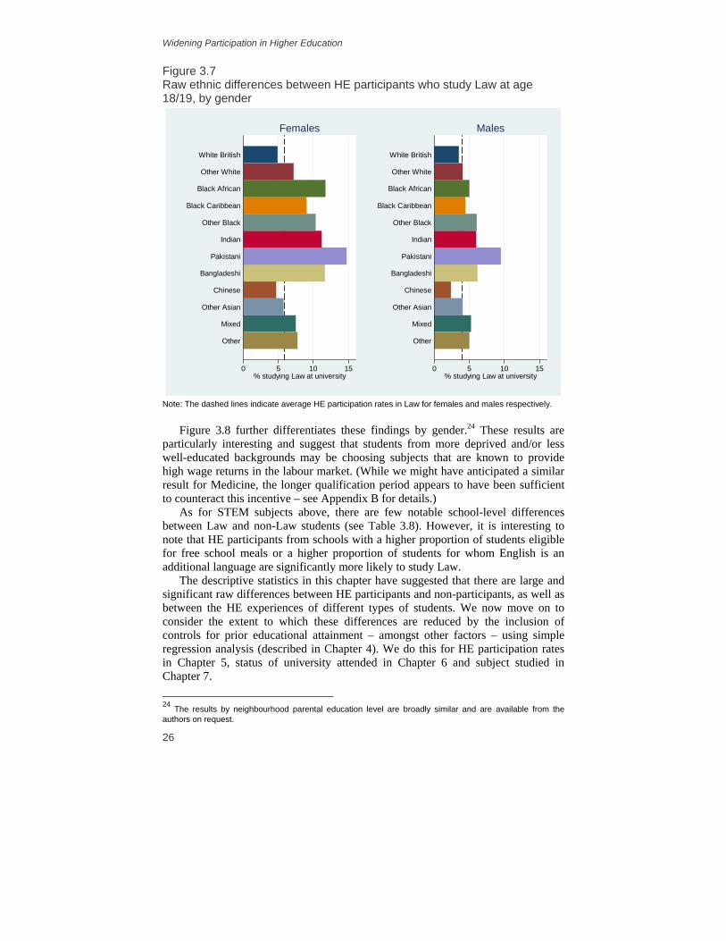
White British students are similarly under-represented: only 68% of Law students are White British compared with 81% in other subjects.23 Figure 3.7 illustrates these differences for males and females separately, and shows that – for female HE participants in particular – a number of ethnic minority groups are well represented in Law, including some groups (e.g. Black Caribbean and Other Black students) that remain under-represented in HE as a whole.
Perhaps more interesting are the differences according to socio-economic background and neighbourhood parental education level. We saw above that HE participants who chose STEM subjects were marginally less deprived and came from marginally better educated neighbourhoods than those who chose other subjects in their first year of university. (This is also true for Maths and Medicine students – see Appendix B.) Law students, on the other hand, are marginally more deprived and come from marginally less well-educated neighbourhoods than those who choose to take other subjects. For example, 10% of HE participants who study Law were eligible for free school meals at age 16 (and 15% were from the 20% most deprived neighbourhoods), compared with 6% (10%) of students who studied other subjects.
23 This is also true for Medicine and (to a lesser extent) for Maths (see Appendix B for details).

Sample Description
25
Table 3.7 Personal characteristics of HE participants who study Law and HE participants who do not Characteristic Study Law In HE but
do not study Law
Difference
Reached expected level at Key Stage 2 0.914 0.909 0.004*** Reached expected level at Key Stage 3 0.946 0.938 0.008*** Achieved 5 A*–C GCSE grades 0.866 0.825 0.041*** Achieved 3 A A-level grades 0.136 0.078 0.058*** Reached Level 3 threshold by 18 via any route 0.973 0.940 0.033*** Eligible for free school meals 0.098 0.062 0.036*** Speaks English as an additional language 0.225 0.123 0.102*** Male 0.348 0.449 –0.100*** White British 0.677 0.808 –0.130*** Other White 0.033 0.029 0.004*** Black African 0.028 0.015 0.013*** Black Caribbean 0.017 0.012 0.006*** Other Black 0.009 0.005 0.004*** Indian 0.094 0.052 0.042*** Pakistani 0.076 0.029 0.047*** Bangladeshi 0.019 0.010 0.009*** Chinese 0.006 0.008 –0.002*** Other Asian 0.005 0.006 0.000 Mixed ethnicity 0.014 0.011 0.003*** Other ethnicity 0.021 0.016 0.005*** Least deprived quintile 0.273 0.315 –0.042*** 2nd deprivation quintile 0.208 0.251 –0.043*** 3rd deprivation quintile 0.203 0.196 0.006*** 4th deprivation quintile 0.164 0.139 0.025*** Most deprived quintile 0.153 0.099 0.053*** Least educated quintile 0.089 0.077 0.012*** 2nd OA education quintile 0.158 0.142 0.016*** 3rd OA education quintile 0.201 0.199 0.002* 4th OA education quintile 0.249 0.256 –0.007*** Most educated quintile 0.303 0.326 –0.023*** Notes: The numbers presented in each column are the mean values of each characteristic for HE participants who study Law (column 1) and HE participants who do not study Law (column 2), and the difference between these means (column 3). For all those characteristics taking values either 0 or 1, the mean values in columns 1 and 2 are interpretable as the proportion of HE participants studying Law or not studying Law who take the value 1 for that characteristic. *** indicates significance at the 1% level, ** at the 5% level and * at the 10% level.
Widening Participation in Higher Education
26
Figure 3.7 Raw ethnic differences between HE participants who study Law at age 18/19, by gender
0 5 10 15% studying Law at university
Other
Mixed
Other Asian
Chinese
Bangladeshi
Pakistani
Indian
Other Black
Black Caribbean
Black African
Other White
White British
Females
0 5 10 15% studying Law at university
Other
Mixed
Other Asian
Chinese
Bangladeshi
Pakistani
Indian
Other Black
Black Caribbean
Black African
Other White
White British
Males
Note: The dashed lines indicate average HE participation rates in Law for females and males respectively.
Figure 3.8 further differentiates these findings by gender.24 These results are particularly interesting and suggest that students from more deprived and/or less well-educated backgrounds may be choosing subjects that are known to provide high wage returns in the labour market. (While we might have anticipated a similar result for Medicine, the longer qualification period appears to have been sufficient to counteract this incentive – see Appendix B for details.)
As for STEM subjects above, there are few notable school-level differences between Law and non-Law students (see Table 3.8). However, it is interesting to note that HE participants from schools with a higher proportion of students eligible for free school meals or a higher proportion of students for whom English is an additional language are significantly more likely to study Law.
The descriptive statistics in this chapter have suggested that there are large and significant raw differences between HE participants and non-participants, as well as between the HE experiences of different types of students. We now move on to consider the extent to which these differences are reduced by the inclusion of controls for prior educational attainment – amongst other factors – using simple regression analysis (described in Chapter 4). We do this for HE participation rates in Chapter 5, status of university attended in Chapter 6 and subject studied in Chapter 7. 24 The results by neighbourhood parental education level are broadly similar and are available from the authors on request.

Sample Description
27
Figure 3.8 Raw socio-economic gap between HE participants who study Law at age 18/19, by gender
0 2 4 6 8 10% studying Law at university
Females
0 2 4 6 8 10% studying Law at university
Males
80% least deprived 20% most deprived
Note: The dashed lines indicate average HE participation rates in Law for females and males respectively.
Table 3.8 Characteristics of schools attended by HE participants who study Law and HE participants who do not Characteristic Study Law In HE but do
not study Law
Difference
Proportion of FSM pupils 0.139 0.117 0.022*** Proportion of EAL pupils 0.135 0.096 0.039*** Proportion of statemented SEN pupils 0.021 0.021 –0.000*** Proportion of non-statemented SEN pupils 0.166 0.159 0.007*** School-level proportion of non-White pupils 0.199 0.154 0.045*** School average capped Key Stage 4 points 37.467 37.837 –0.369*** Is a community school 0.588 0.576 0.012*** Is a foundation school 0.188 0.190 –0.002* Is a voluntary aided school 0.180 0.182 –0.002 Is a voluntary controlled school 0.036 0.044 –0.008*** Notes: See Notes to Table 3.7. *** indicates significance at the 1% level, ** at the 5% level and * at the 10% level.

28
CHAPTER 4 Methodology
Our modelling approach is based on a linear probability regression model in which we explore the determinants of: first, HE participation generally; second, HE participation in a high-status institution; and third, HE participation in a particular subject or subject group.25 The dependent variables for our three sets of models are therefore binary, taking a value of 1 if the person participates and 0 otherwise.
The regression model is estimated using ordinary least squares (OLS) and is as follows:
1 2 3 4is i i s i i sHE SEG X S PAα β β β β µ η= + + + + + +
where SEG represents the characteristic of interest (either material deprivation, ethnicity or a neighbourhood-level proxy for parental education), X is a vector of other individual characteristics, S is a limited vector of characteristics of the individual’s school (at age 16), PA measures the individual’s prior achievement (from age 11 to age 18) and µi is a normally distributed error term. As discussed in Chapter 2, we include only limited school characteristics and do not measure school quality directly but rather include a dummy variable for each school in our sample, thereby focusing on differences in HE participation rates across different types of student within the same school at age 16 (as shown above, where ηs is a school fixed effect). We adopt this fixed effects methodology rather than a random effects approach (or multi-level model, as it is known in the education literature) because the explanatory variables included in the model are likely to be correlated with the school effects, thus rendering the random effects model inappropriate. However, we do allow for clustering within schools in our standard errors. Adopting a fixed effects rather than a random effects approach changes the value of the coefficients on explanatory variables of interest (thus justifying the fixed effects approach). However, further research exploring the different modelling approaches when using population administrative data is an important avenue for future education research that we are pursuing.
The model is estimated using OLS since we have a large number of school fixed effects to estimate and the model becomes unwieldy in STATA when we use a probit. However, to verify robustness, we have estimated some models using a probit, with very similar results (available on request).
We first estimate the model with no controls, to estimate the raw differences in HE participation at age 18 or 19 between groups of young people, classified according to material deprivation, neighbourhood parental education and ethnicity (described graphically in Chapter 3 – see Figures 3.1–3.3). We then examine the extent to which these gaps can be explained away by differences in other observable characteristics. 25 The only exception comes when we use an ordered logit model to investigate the effects of material deprivation, neighbourhood parental education and ethnicity on subject studied according to wage return in the labour market. We discuss this model in more detail in Section 7.3.

Methodology
29
The model is estimated sequentially. We start by including secondary school fixed effects, to investigate the extent to which differences in HE participation rates stem from differences in the quality of secondary schools to which different types of pupils have access; these form our baseline estimates. Controlling for school quality is important in our model because if, for example, pupils from more materially deprived backgrounds are more likely to attend poorly performing schools than those from less materially deprived backgrounds, then by comparing pupils across schools we are essentially conflating the impact of material deprivation with the impact of the quality of secondary school attended. In this case, we would expect the across-schools model to overstate the direct impact of material deprivation on HE participation rates. Of course, in interpreting these results we must be aware that fully identifying the effects of school quality on HE participation is a difficult task and one that is beyond the scope of this report. In particular, our methods do not allow us to separate the effects of school quality from either peer effects or the effects of any unobserved differences between pupils that are correlated with both their choice of school and their HE decision.26 Moreover, material deprivation is likely to affect the quality of secondary school attended and thus may be one route through which disadvantaged pupils end up with lower achievement.
We then move on to include variables describing the personal characteristics of the individual (in particular, month of birth, special educational needs status and whether the pupil has English as an additional language). Finally, we add in measures of prior attainment – Key Stage 2 results (age 11), Key Stage 3 results (age 14), Key Stage 4 results (age 16) and Key Stage 5 results (age 18).27 We do this in order to better understand whether material deprivation, neighbourhood parental education and ethnicity affect HE participation rates directly, or through their impact on prior attainment (which in turn affects the likelihood of attending university), or both.
We use the term ‘impact’ in this report to describe the statistical association between material deprivation, neighbourhood educational levels and ethnicity, and the probability of attending HE at the age of 18 or 19. We would obviously like to uncover the causal effects of material deprivation (and our other characteristics of interest) on HE attendance; however, in the absence of any experiment or quasi-experiment, the regression methodology we adopt has a potential weakness – namely, omitted variable bias. To determine the causal impact of material deprivation on the likelihood of HE participation, we need to be sure that we have controlled for the range of other factors that influence participation. For instance, we know that individuals from certain ethnic minority groups have higher levels of educational achievement. As ethnicity and socio-economic background are correlated, we must control for ethnicity in order to recover the causal effect of material deprivation on HE participation; otherwise, what appears to be an effect from socio-economic background may actually be an effect from ethnicity.28
26 For a fuller discussion of the difficulties in measuring the effects of school quality on pupil attainment and decisions, see Card and Krueger (1992). 27 Of course, we do not have Key Stage 5 results for all pupils, as some will have chosen not to stay on in education beyond age 16. For these individuals, we include a missing Key Stage 5 results dummy and ascribe them a Key Stage 5 score of zero. 28 See Haveman and Wolfe (1995) for a survey of literature that attempts to identify the causal effects of material deprivation on HE participation.
Widening Participation in Higher Education
30
To the extent that there are factors that influence HE participation that are unobserved in our data, we may not be uncovering a causal relationship. However, the strength of our analysis is that we have longitudinal data on educational performance and achievement. By controlling for prior achievement, we are better able to allow for unobservable factors that influence educational achievement, assuming that such unobserved factors are likely to influence earlier achievement as well as the HE participation decision.
Another issue we face in our analysis is that some individuals delay participation in HE beyond the age of 19. We do not have data on participation beyond age 19; thus our estimates of participation rates will understate HE participation for some students. To the extent that poorer or ethnic minority students are more (less) likely to delay participation, we will tend to over- (under-) state the gap in HE participation between richer and poorer students, and under- (over-) state the positive gap in HE participation between some ethnic minority students and White British students.
The final, but crucially important, caveat is that we only observe state school pupils. We know from other work that children who attend fee-paying (private or independent) schools are more likely to participate in higher education.29 Obviously, children who attend fee-paying schools also tend to come from more advantaged families. If we were to include such children in the analysis, it is almost certain that the raw socio-economic gap in HE participation would be larger still. If, as is likely, children at fee-paying schools also have higher HE participation rates for a given level of prior achievement, it will also be the case that the conditional socio-economic gap in HE participation would be larger if these children were included in our sample. Furthermore, children at fee-paying schools are disproportionately more likely to attend a high-status HEI, so our estimates of the socio-economic gap in HE participation in a high-status HEI (Chapter 6) may be particularly affected.30 Since we do not have sufficient information on private school children to include them in the analysis, we simply point out to the reader that our results pertain to state school children only.
29 In our data, individuals for whom we observe Key Stage 4 results (but not PLASC data) are likely to attend private schools. Interestingly, if we calculate the HE participation rate for individuals falling into this category, it does not differ very much from the HE participation rate observed amongst state school pupils, being 32.0% (compared with 29.6% for our sample of state school students). 30 Sutton Trust (2008) documents the extent to which a few highly socially and academically selective schools dominate admissions to the country’s leading research universities.

31
CHAPTER 5 Participation in Higher Education
In this chapter, we consider the associations between material deprivation, parental education and ethnicity, and participation in higher education at age 18 or 19. More specifically, we estimate the impact of being amongst the 20% most materially deprived secondary school pupils (compared with other quintiles), the impact of being amongst the 20% of secondary school pupils living in the least well-educated neighbourhoods (compared with other quintiles) and the impact of being of Other White, Black African, Black Caribbean, Other Black, Indian, Pakistani, Bangladeshi, Chinese, Other Asian, Mixed or Other ethnic origin (compared with White British ethnic origin).31 Due to the well-established differences in educational attainment by gender, we do this separately for males and females.
In Section 5.1, we report the raw differences in HE participation rates by material deprivation, neighbourhood parental education and ethnicity, and show how these gaps change once school quality and other individual-level characteristics are included in the model. In Section 5.2, we go on to illustrate how these estimates alter once we add in academic attainment from age 11 through to age 18. In Section 5.3, we examine the impact of prior attainment on HE participation rates in more detail, by considering how changes in attainment over time (specifically, between Key Stage 2 and Key Stage 4) affect the likelihood of going on to university at age 18 or 19. Section 5.4 offers some brief conclusions.
5.1 Baseline estimates of differences in HE participation rates
In this section, we discuss estimates of the impact of material deprivation,32 neighbourhood parental education and ethnicity on the likelihood of participating in higher education at age 18 or 19 for males (Section 5.1.1) and females (Section 5.1.2). For each factor, we present both raw differences (across schools) and estimates controlling for school quality (within schools).
5.1.1 Males Table 5.1 presents estimates of the impact of material deprivation, neighbourhood parental education and ethnicity on the likelihood of going to university at age 18 or 19 for males. It is clear from this table that both material deprivation and low neighbourhood parental education are associated with low HE participation rates
31 We use the term ‘impact’ in this chapter to describe the statistical association between material deprivation (and other factors) and the probability of attending HE at the age of 18 or 19. 32 Results using FSM status alone (rather than an index of material deprivation, of which FSM status is one component) are broadly similar to the main results discussed throughout this chapter. These results are available from the authors on request.

Widening Participation in Higher Education
32
amongst boys. For example, being among the 20% least materially deprived pupils (compared with the 20% most materially deprived pupils) more than trebles the likelihood of going to university, from 12.7% to 41.7% (a gap of 29.0 percentage points). Similarly, being among the 20% of pupils living in the best-educated neighbourhoods (compared with the 20% of pupils from the least well-educated neighbourhoods) more than quadruples the probability of HE participation, from 9.2% to 43.8% (a gap of 34.6 percentage points). Once we take school quality into account (by including secondary school fixed effects), these gaps fall to 24.1 percentage points and 25.6 percentage points respectively, suggesting that materially deprived pupils and pupils living in poorly educated neighbourhoods are more likely to attend poorly performing secondary schools than non-materially-deprived pupils and pupils in highly educated neighbourhoods.33 This means that increasing HE participation rates amongst these pupils may, at least partly, be achieved by providing greater access to better secondary schools.
The raw findings from Table 5.1 indicate that boys from most ethnic minority subgroups are significantly more likely to go to university at age 18 or 19 than White British boys. These differences are largest for pupils of Indian (34.2 percentage points), Chinese (38.4 percentage points), Other Asian (51.1 percentage points) and Mixed (34.9 percentage points) ethnic origin. Boys of Black Caribbean and Other Black ethnic origin are the only groups that are significantly less likely to participate in HE than White British boys, with gaps of 6.1 and 6.2 percentage points respectively. This finding is consistent with recent research that suggested that the educational achievement of some groups of ethnic minority students exceeds that of White British students (Wilson, Burgess and Briggs, 2005).
Once we compare pupils of different ethnic origins within the same schools, some interesting patterns emerge. It appears that boys of Black, Pakistani, Bangladeshi or Other ethnic origin are more likely to attend poorly performing schools than White British boys, while boys of Other White, Indian, Chinese, Other Asian or Mixed ethnic origin are more likely to attend high-performing schools than White British boys. We make these inferences on the basis that forcing comparisons within schools favourably affects the participation rates of boys of Black, Pakistani, Bangladeshi or Other ethnic origin relative to White British boys, but harms the participation rates of boys of Other White, Indian, Chinese, Other Asian or Mixed ethnic origin relative to White British boys. For example, while the raw results suggest that boys of Other Asian ethnic origin are 51.1 percentage points more likely to participate in HE at age 18 or 19 than White British boys, they are only 38.9 percentage points more likely to participate once we control for school quality.
33 These raw differences are considerably larger than those found for age 18 HE participation alone (see Chowdry et al. (2008)). In terms of material deprivation, this appears to be primarily the result of an increase in the base, i.e. an increase in the participation rate amongst individuals who live in one of the 20% most deprived neighbourhoods. This suggests that, amongst state school pupils at least, those who delay HE participation by a year are relatively more deprived than those who elect to go to university straightaway, perhaps suggesting a role for A-level (or equivalent) retakes. This is borne out by comparing the characteristics of participants who started university in 2004–05 (at age 18) with those who started in 2005–06 (at age 19) – see Appendix C for details.

Participation in Higher Education
33
Table 5.1 Raw gradients in HE participation rates for males, by deprivation quintile, neighbourhood parental education quintile and ethnicity Material deprivation Neighbourhood
parental education Ethnicity
Across schools
Within schools
Across schools
Within schools
Across schools
Within schools
4th deprivation quintile
0.049*** 0.049***
3rd deprivation quintile
0.124*** 0.116***
2nd deprivation quintile
0.196*** 0.175***
Least deprived quintile
0.290*** 0.241***
2nd OA education quintile
0.087*** 0.064***
3rd OA education quintile
0.161*** 0.121***
4th OA education quintile
0.240*** 0.178***
Most educated quintile
0.346*** 0.256***
Other White 0.053*** 0.038*** Black African 0.070*** 0.116*** Black Caribbean –0.061*** –0.009 Other Black –0.062*** –0.018* Indian 0.342*** 0.328*** Pakistani 0.092*** 0.171*** Bangladeshi 0.055*** 0.145*** Chinese 0.384*** 0.336*** Other Asian 0.511*** 0.389*** Mixed ethnicity 0.349*** 0.273*** Other ethnicity 0.026*** 0.049***
Constant 0.127*** 0.143*** 0.092*** 0.135*** 0.242*** 0.238*** Observations 262,516 262,516 262,516 262,516 262,516 262,516 R-squared 0.056 0.055 0.074 0.074 0.025 0.023 No. of clusters 3,452 3,452 3,452 Note: The within-schools specification includes school fixed effects (using school attended at age 16). *** indicates significance at the 1% level, ** at the 5% level and * at the 10% level.
Table 5.2 extends this analysis by controlling for material deprivation, neighbourhood parental education and ethnicity in the same model (within schools). Given the likely correlation between low neighbourhood parental education and high material deprivation, it is not surprising to see that the estimated impacts of each factor fall once we control for both measures in the same model. For example,

Widening Participation in Higher Education
34
while the results controlling for school quality alone suggest that boys amongst the 20% of secondary school pupils who live in the most highly educated neighbourhoods were 25.6 percentage points more likely to go on to university than boys amongst the 20% of pupils from the least highly educated neighbourhoods, once we control for material deprivation and ethnicity as well this disparity falls to 16.8 percentage points.
Table 5.2 Gradients in HE participation rates for males, controlling for individual-level characteristics (excluding prior attainment) Controlling for
deprivation, neighbourhood
parental educationand ethnicity
Plus other individual-level characteristics
4th deprivation quintile 0.032*** 0.022*** 3rd deprivation quintile 0.081*** 0.064*** 2nd deprivation quintile 0.124*** 0.102*** Least deprived quintile 0.169*** 0.143***
2nd OA education quintile 0.031*** 0.027*** 3rd OA education quintile 0.063*** 0.055*** 4th OA education quintile 0.103*** 0.093*** Most educated quintile 0.168*** 0.156***
Other White 0.038*** 0.020** Black African 0.133*** 0.096*** Black Caribbean 0.009 0.018*** Other Black 0.000 0.001 Indian 0.321*** 0.263*** Pakistani 0.188*** 0.136*** Bangladeshi 0.166*** 0.106*** Chinese 0.328*** 0.273*** Other Asian 0.390*** 0.337*** Mixed ethnicity 0.276*** 0.256*** Other ethnicity 0.059*** 0.032***
Constant 0.083*** 0.146*** Observations 262,516 262,516 R-squared 0.111 0.143 No. of clusters 3,452 3,452 F-test of additional controls (p-value) 0 0 Notes: All models include school fixed effects (on the basis of school attended at age 16). In addition to deprivation quintile, neighbourhood parental education quintile and ethnicity, column 2 also includes controls for month of birth, whether English is the pupil’s first language and whether they have either statemented (more severe) or non-statemented (less severe) special educational needs (measured at age 16). *** indicates significance at the 1% level, ** at the 5% level and * at the 10% level.

Participation in Higher Education
35
Controlling for material deprivation and neighbourhood parental education has a generally smaller impact on the ethnicity coefficients in our model, although it appears to affect different ethnic groups in different ways. For example, amongst Indian and Chinese boys, controlling for material deprivation and neighbourhood parental education marginally reduces the advantage that they have over White British boys in terms of HE participation rates. On the other hand, amongst boys of all other ethnic origins (excluding Other White boys, for whom the coefficient does not change), additionally controlling for these factors increases the advantage (or reduces the disadvantage) that they face relative to White British boys. This suggests that Indian and Chinese boys are less materially deprived and/or live in neighbourhoods with better-educated parents than White British boys, while the reverse is true for boys of other ethnic origins (excluding Other White).34
The results reported in the second column of Table 5.2 also control for month of birth, whether English is an additional language for the pupil and special educational needs status. These figures show an almost universal reduction in the absolute values of the estimates of the impact of material deprivation, neighbourhood parental education and ethnicity on HE participation rates at age 18 or 19.35 For example, controlling for these additional factors reduces the gap in participation rates between boys of Bangladeshi and White British ethnic origin by 6 percentage points (from 16.6 to 10.6 percentage points).
5.1.2 Females Table 5.3 provides estimates of the impact of material deprivation, neighbourhood parental education and ethnicity on the likelihood of going to university at age 18 or 19 for girls, with (within schools) and without (across schools) controls for school quality. These figures exhibit a largely similar pattern to those found for boys (see Section 5.1.1), with the exception that the point estimates of the gap between different types of female students tend to be larger.36 However, because the base also tends to be higher for females than for males, the difference in percentage terms is often much smaller. For example, the raw results show that girls among the 20% least materially deprived secondary school pupils are, on average, 34.6 percentage points more likely to participate in higher education at age 18 or 19 than girls among the 20% most materially deprived secondary school pupils; this compares with a difference of 29.0 percentage points for boys. In percentage terms, however, girls and boys from the least materially deprived quintile are both around three times more likely to go on to university at age 18 or 19 than girls and boys from the most materially deprived quintile.
Interestingly, while the raw differences suggest that neighbourhood parental education has a greater impact on female HE participation rates than material deprivation, the effects are very similar once we compare girls who attend the same school. For example, the raw results show that girls amongst the 20% least 34 The same is also true for girls from these groups – except that the advantage of Other White girls increases once controls for material deprivation and neighbourhood parental education are included (see Tables 5.3 and 5.4 for details). 35 The exceptions are for Black Caribbean and Other Black boys, for whom the point estimates marginally increase (from 0.009 to 0.018 and from 0.000 to 0.001 respectively). 36 Notable exceptions are for individuals of Pakistani, Chinese, Other Asian and Mixed ethnic origin, for whom the differences relative to White British individuals are slightly larger for boys than they are for girls.

Widening Participation in Higher Education
36
materially deprived secondary school pupils are 34.6 percentage points more likely to start university at age 18 or 19 than girls amongst the 20% most materially deprived pupils, while girls amongst the 20% of pupils who live in the most highly educated neighbourhoods are 39.9 percentage points more likely to participate in Table 5.3 Raw gradients in HE participation rates for females, by deprivation quintile, neighbourhood parental education quintile and ethnicity Material deprivation Neighbourhood
parental education Ethnicity
Across schools
Within schools
Across schools
Within schools
Across schools
Within schools
4th deprivation quintile
0.067*** 0.072***
3rd deprivation quintile
0.161*** 0.158***
2nd deprivation quintile
0.245*** 0.231***
Least deprived quintile
0.346*** 0.306***
2nd OA education quintile
0.106*** 0.082***
3rd OA education quintile
0.202*** 0.157***
4th OA education quintile
0.294*** 0.227***
Most educated quintile
0.399*** 0.302***
Other White 0.062*** 0.039*** Black African 0.127*** 0.183*** Black Caribbean –0.008 0.049*** Other Black –0.044*** 0.006 Indian 0.363*** 0.355*** Pakistani 0.073*** 0.161*** Bangladeshi 0.053*** 0.158*** Chinese 0.355*** 0.312*** Other Asian 0.444*** 0.349*** Mixed ethnicity 0.344*** 0.262*** Other ethnicity 0.039*** 0.058***
Constant 0.172*** 0.183*** 0.136*** 0.182*** 0.316*** 0.312*** Observations 254,512 254,512 254,512 254,512 254,512 254,512 R-squared 0.068 0.068 0.088 0.088 0.023 0.021 No. of clusters 3,381 3,381 3,381 Note: The within-schools specification includes school fixed effects (using school attended at age 16). *** indicates significance at the 1% level, ** at the 5% level and * at the 10% level.

Participation in Higher Education
37
Table 5.4 Gradients in HE participation rates for females, controlling for individual-level characteristics (excluding prior attainment) Controlling for
deprivation, neighbourhood
parental educationand ethnicity
Plus other individual-level characteristics
4th deprivation quintile 0.053*** 0.042*** 3rd deprivation quintile 0.118*** 0.101*** 2nd deprivation quintile 0.168*** 0.148*** Least deprived quintile 0.219*** 0.196***
2nd OA education quintile 0.038*** 0.033*** 3rd OA education quintile 0.083*** 0.077*** 4th OA education quintile 0.132*** 0.123*** Most educated quintile 0.191*** 0.181***
Other White 0.043*** 0.025** Black African 0.209*** 0.165*** Black Caribbean 0.073*** 0.078*** Other Black 0.029** 0.027** Indian 0.343*** 0.279*** Pakistani 0.182*** 0.121*** Bangladeshi 0.190*** 0.124*** Chinese 0.305*** 0.250*** Other Asian 0.354*** 0.298*** Mixed ethnicity 0.268*** 0.248*** Other ethnicity 0.074*** 0.046***
Constant 0.112*** 0.160*** Observations 254,512 254,512 R-squared 0.125 0.148 No. of clusters 3,381 3,381 F-test of additional controls (p-value) 0 0 Notes: All models include school fixed effects (on the basis of school attended at age 16). In addition to deprivation quintile, neighbourhood parental education quintile and ethnicity, column 2 also includes controls for month of birth, whether English is the pupil’s first language and whether they have either statemented (more severe) or non-statemented (less severe) special educational needs (measured at age 16). *** indicates significance at the 1% level, ** at the 5% level and * at the 10% level.
HE than girls amongst the 20% of pupils who live in the most poorly educated neighbourhoods. Once we control for school quality, however, these differences fall to 30.6 percentage points and 30.2 percentage points respectively. (A similar pattern is also evident for boys – see Table 5.1.)
In terms of ethnicity, two groups are worthy of note: while Black African girls seem to perform much better (relative to White British girls) than do Black African

Widening Participation in Higher Education
38
boys (relative to White British boys), boys of Other Asian ethnic origin outperform White British boys to a greater extent than girls of Other Asian ethnic origin outperform White British girls. Table 5.3 shows that Black African girls are 12.7 percentage points more likely to participate in HE at age 18 or 19 than White British girls (using the across-schools model) and 18.3 percentage points more likely to participate once we add in controls for school quality (the within-schools model). This compares with differences (shown in Table 5.1) of 7.0 percentage points between Black African and White British boys in the raw results and of 11.6 percentage points once we allow for the effects of school quality. By contrast, girls of Other Asian ethnic origin are 44.4 (34.9) percentage points more likely to go on to university than White British girls in the across- (within-) schools model, while the premium for Other Asian boys (compared with White British boys) is 51.1 (38.9) percentage points.
Table 5.4 illustrates how estimates of the impact of material deprivation, neighbourhood parental education and ethnicity change once we control for all three factors in the same model (first column) and after including other individual-level characteristics (second column). In both cases, the changes observed for girls closely parallel those for boys (see Section 5.1.1 for details).
5.2 The importance of prior attainment
In this section, we move on to consider how the inclusion of successive measures of prior educational attainment (starting with Key Stage 2 and ending with Key Stage 537) affects our estimates of the impact of material deprivation, neighbourhood parental education and ethnicity on HE participation rates using the within-schools model. We do this for males (Table 5.5) and females (Table 5.6) separately, but discuss the results simultaneously. The first column of each table replicates the results shown in the second column of Tables 5.2 (for males) and 5.4 (for females), i.e. it presents estimates of the impact of material deprivation, neighbourhood parental education and ethnicity on HE participation rates, having controlled for school quality, month of birth, whether English is the pupil’s first language and whether they have special educational needs. Columns 2 through 5 go on to illustrate how these estimates change once we add in Key Stage 2 results (age 11), Key Stage 3 results (age 14), Key Stage 4 results (age 16) and Key Stage 5 results (age 18). By doing this, we show how HE participation rates differ across different types of student with the same pattern of earlier attainment.
As might be expected, the inclusion of controls for prior educational attainment reduces the effects of both material deprivation and neighbourhood parental education on HE participation rates. For example, the impact (on the likelihood of going on to university at age 18 or 19) of being amongst the 20% of pupils from the least materially deprived backgrounds (compared with the 20% of pupils from the most materially deprived backgrounds) falls from 14.3 to 10.5 percentage points for boys – and from 19.6 to 14.1 percentage points for girls – once we add in Key Stage 2 results. This suggests that socio-economic disadvantage has already made an
37 We include a missing dummy for all individuals for whom we do not observe Key Stage 5 results.

Participation in Higher Education
39
impact on academic outcomes at the age of 11 and that this disadvantage can explain a significant proportion of the gap in HE participation at age 18 or 19.38
Table 5.5 Gradients in HE participation for males, controlling for individual-level characteristics and prior attainment Individual-
level controls
Plus Key Stage 2 results
Plus Key Stage 3 results
Plus Key Stage 4 results
Plus Key Stage 5 results
4th deprivation quintile 0.022*** 0.013*** 0.008*** 0.000 0.000 3rd deprivation quintile 0.064*** 0.043*** 0.027*** 0.008*** 0.001 2nd deprivation quintile 0.102*** 0.072*** 0.049*** 0.019*** 0.003 Least deprived quintile 0.143*** 0.105*** 0.073*** 0.032*** 0.010***
2nd OA education quintile 0.027*** 0.019*** 0.013*** 0.006*** 0.004** 3rd OA education quintile 0.055*** 0.040*** 0.028*** 0.014*** 0.006*** 4th OA education quintile 0.093*** 0.069*** 0.051*** 0.029*** 0.013*** Most educated quintile 0.156*** 0.120*** 0.091*** 0.056*** 0.030***
Other White 0.020** 0.035*** 0.032*** 0.021*** 0.014*** Black African 0.096*** 0.131*** 0.139*** 0.113*** 0.086*** Black Caribbean 0.018*** 0.048*** 0.064*** 0.063*** 0.050*** Other Black 0.001 0.029*** 0.040*** 0.043*** 0.038*** Indian 0.263*** 0.279*** 0.256*** 0.204*** 0.148*** Pakistani 0.136*** 0.162*** 0.160*** 0.131*** 0.099*** Bangladeshi 0.106*** 0.120*** 0.110*** 0.075*** 0.063*** Chinese 0.273*** 0.263*** 0.212*** 0.161*** 0.113*** Other Asian 0.337*** 0.338*** 0.288*** 0.201*** 0.128*** Mixed ethnicity 0.256*** 0.227*** 0.197*** 0.134*** 0.063*** Other ethnicity 0.032*** 0.055*** 0.058*** 0.048*** 0.043***
Constant 0.146*** 0.006 –0.027*** –0.031*** 0.067*** Observations 262,516 262,516 262,516 262,516 262,516 R-squared 0.143 0.252 0.333 0.436 0.579 No. of clusters 3,452 3,452 3,452 3,452 3,452 F-test of additional controls (p-value)
0 0 0 0 0
Notes: The results presented in column 1 replicate those found in column 2 of Table 5.2. All models are within-school. *** indicates significance at the 1% level, ** at the 5% level and * at the 10% level.
38 Unfortunately, our data do not contain earlier test results, making it impossible to assess when these differences in attainment (by socio-economic status) first emerge for our cohort. However, it is worth noting that much of the recent literature suggests that it is likely to have been significantly earlier than age 11 (see, for example, Cunha and Heckman (2007)).

Widening Participation in Higher Education
40
Table 5.6 Gradients in HE participation rates for females, controlling for individual-level characteristics and prior attainment Individual-
level controls
Plus Key Stage 2 results
Plus Key Stage 3 results
Plus Key Stage 4 results
Plus Key Stage 5 results
4th deprivation quintile 0.042*** 0.028*** 0.017*** 0.006*** 0.002 3rd deprivation quintile 0.101*** 0.070*** 0.046*** 0.020*** 0.008*** 2nd deprivation quintile 0.148*** 0.106*** 0.073*** 0.034*** 0.013*** Least deprived quintile 0.196*** 0.141*** 0.099*** 0.050*** 0.021***
2nd OA education quintile 0.033*** 0.020*** 0.013*** 0.005** 0.001 3rd OA education quintile 0.077*** 0.054*** 0.040*** 0.024*** 0.011*** 4th OA education quintile 0.123*** 0.089*** 0.067*** 0.042*** 0.021*** Most educated quintile 0.181*** 0.136*** 0.103*** 0.066*** 0.032***
Other White 0.025** 0.045*** 0.047*** 0.025*** 0.021*** Black African 0.165*** 0.199*** 0.205*** 0.168*** 0.122*** Black Caribbean 0.078*** 0.113*** 0.126*** 0.112*** 0.084*** Other Black 0.027** 0.052*** 0.064*** 0.058*** 0.045*** Indian 0.279*** 0.290*** 0.259*** 0.206*** 0.158*** Pakistani 0.121*** 0.154*** 0.153*** 0.114*** 0.087*** Bangladeshi 0.124*** 0.148*** 0.134*** 0.083*** 0.067*** Chinese 0.250*** 0.248*** 0.181*** 0.121*** 0.080*** Other Asian 0.298*** 0.305*** 0.251*** 0.170*** 0.107*** Mixed ethnicity 0.248*** 0.218*** 0.187*** 0.138*** 0.068*** Other ethnicity 0.046*** 0.068*** 0.065*** 0.046*** 0.046***
Constant 0.160*** –0.005 –0.033*** –0.027*** 0.087*** Observations 254,512 254,512 254,512 254,512 254,512 R-squared 0.148 0.260 0.339 0.436 0.571 No. of clusters 3,381 3,381 3,381 3,381 3,381 F-test of additional controls (p-value)
0 0 0 0 0
Notes: The results presented in column 1 replicate those found in column 2 of Table 5.4. All models are within-school. *** indicates significance at the 1% level, ** at the 5% level and * at the 10% level.
It is worth noting, however, that at each Key Stage, the impact of material deprivation on HE participation is reduced by more than the impact of neighbourhood parental education on the same outcome. For example, the inclusion of Key Stage 3 test results reduces the premium associated with being amongst the 20% least materially deprived secondary school pupils (compared with the 20% most materially deprived pupils) for both males and females by around 30%;39
39 For boys: (10.5–7.3)/10.5=30.5%. For girls: (14.1–9.9)/14.1=29.8%. All other percentages cited in this section are calculated in a similar fashion.

Participation in Higher Education
41
however, it reduces the effect associated with living in one of the most highly educated neighbourhoods (compared with one of the most poorly educated neighbourhoods) by only around 24%. This suggests that material deprivation may be a better predictor of prior attainment than neighbourhood parental education. (Of course, this may be at least partly explained by the fact that we only have a local area proxy for parental education.)
The explanatory power of prior attainment also increases with each successive Key Stage: that is to say, the coefficients on material deprivation and neighbourhood parental education are reduced more as a result of the inclusion of later Key Stages than they are as a result of the inclusion of earlier Key Stages. For example, while the coefficients on material deprivation were reduced by around 30% for both boys and girls following the inclusion of Key Stage 2 and Key Stage 3 results, they were reduced by around 50% for girls and 60% for boys when we added Key Stage 4 (GCSE) results and by around 60% for girls and 70% for boys when we added Key Stage 5 (A-level and equivalent) results. This suggests that an important part of the HE participation story is what happens to the academic trajectories of the most disadvantaged students between the ages of 11 and 16 (and consequently whether they choose to stay on beyond compulsory schooling). We consider this issue in more detail in Section 5.3.
Once we have added in all available measures of prior attainment (i.e. up to Key Stage 5), there is little evidence of any sizeable association between material deprivation or neighbourhood parental education and HE participation rates. In particular, boys (girls) amongst the 20% of pupils who are least materially deprived are now only 1.0 (2.1) percentage points more likely to go on to university at age 18 or 19 than boys (girls) amongst the 20% of pupils who are most materially deprived; this compares with a raw difference of 29.0 (34.6) percentage points. Similarly, boys (girls) amongst the 20% of pupils from the most well-educated neighbourhoods are now only 3.0 (3.2) percentage points more likely to participate in HE than boys (girls) amongst the 20% of pupils from the least well-educated neighbourhoods; this compares with a raw difference of 34.6 (39.9) percentage points.
Taken together, these results indicate that for individuals from poorer socio-economic backgrounds (including those facing material deprivation and those from poorly educated neighbourhoods), the inclusion of prior educational attainment – particularly Key Stage 4 and Key Stage 5 results – significantly reduces the HE participation gap. This suggests that one of the main challenges to widening participation in higher education for these groups is to increase the proportion of pupils getting good GCSE and A-level (or equivalent) results.
Turning our attention now to the impact of ethnicity on the likelihood of going to university at age 18 or 19, it is interesting to note that for all ethnic minority groups except those of Chinese or Mixed ethnic origin, the inclusion of Key Stage 2 results actually increases the impact of ethnicity on HE participation rates, such that all ethnic minority groups are now, on average, significantly more likely to go to university than White British students. For example, Black African boys are, on average, 9.6 percentage points more likely (than White British boys) to go to university before the inclusion of Key Stage 2 results and 13.1 percentage points more likely thereafter. Similarly, Black African girls are 16.5 percentage points
Widening Participation in Higher Education
42
more likely to go to university (than White British girls) before the inclusion of Key Stage 2 results and 19.9 percentage points more likely thereafter.
For boys and girls of Black ethnic origin, this effect persists following the inclusion of Key Stage 3 results. For example, while the participation gap between Black Caribbean and White British boys is 4.8 percentage points before the inclusion of Key Stage 3 results, it increases to 6.4 percentage points thereafter. However, other ethnic groups generally experience a relative reduction in their HE participation advantage: for example, for Chinese boys, an advantage of 26.3 percentage points over White British boys before the inclusion of Key Stage 3 results is reduced to 21.2 percentage points thereafter.
Once we start adding in Key Stage 4 and Key Stage 5 results, however, the effect of including prior attainment is almost unambiguously to reduce the participation gap between ethnic minority and White British students. For example, Black African boys are 13.9 percentage points more likely to participate in higher education at age 18 or 19 than White British boys when we control for Key Stage 2 and Key Stage 3 results, but this advantage falls to 11.3 percentage points once we include GCSE results and to 8.6 percentage points once we include A-level (or equivalent) results. Similarly, a gap of 20.5 percentage points for Black African girls using Key Stage 2 and Key Stage 3 results as controls falls to 16.8 percentage points and then to 12.2 percentage points once we include Key Stage 4 and then Key Stage 5 results respectively.
The fact that, for most ethnic minority groups, the inclusion of Key Stage 2 results seems to increase the observed participation gap, while the inclusion of Key Stage 4 results seems to reduce it, suggests that the attainment of ethnic minority students may rise relative to that of White British students between the ages of 11 and 16. This is supported by findings from Wilson, Burgess and Briggs (2005). Furthermore, given that the majority of raw results suggest that significantly more ethnic minorities than White British students go to university at age 18 or 19, perhaps the issue of widening participation in this context is more to do with increasing the participation of White British students at these ages.40
5.3 Changes in attainment over time and HE participation rates
In this section, we consider the impact of changes in attainment over time on HE participation rates for selected subgroups. Specifically, we split the population up into quintiles according to their Key Stage 2 and Key Stage 4 results, and then plot one against the other – to show how the academic achievement of various subgroups evolves over time and to highlight how this progression affects the likelihood of going to university at age 18 or 19. We do this separately for males and females, but we discuss the results together.
40 Of course, ethnic differences in the status of HE institution accessed may also be important. We consider this issue in Chapter 6 of this report.

Participation in Higher Education
43
Table 5.7 Transition matrix showing changes in attainment over time for males amongst the 20% most materially deprived pupils Key Stage 4
Key Stage 2 Lowest scores
Quintile 2
Quintile 3
Quintile 4
Highest scores Total
Lowest scores 8,588 3,562 924 140 26 13,240 64.9 26.9 7.0 1.1 0.2 100.0 0.9 8.8 33.2 60.0 65.4 6.1
Quintile 2 3,172 3,679 1,869 418 92 9,230 34.4 39.9 20.2 4.5 1.0 100.0 0.9 6.1 27.3 58.6 75.0 11.7
Quintile 3 1,373 2,336 2,204 771 200 6,884 19.9 33.9 32.0 11.2 2.9 100.0 0.9 4.9 22.8 49.7 78.5 17.0
Quintile 4 564 1,099 1,710 1,067 463 4,903 11.5 22.4 34.9 21.8 9.4 100.0 0.9 5.7 22.0 49.8 72.1 26.7
Highest scores 165 359 858 995 927 3,304 5.0 10.9 26.0 30.1 28.1 100.0 2.4 4.7 16.1 45.2 79.4 40.7 Total 13,862 11,035 7,565 3,391 1,708 37,561 36.9 29.4 20.1 9.0 4.5 100.0 0.9 6.7 24.3 49.9 76.9 15.2 Notes: Numbers in bold italics represent the percentage of individuals in a given quintile at Key Stage 2 who appear in each quintile at Key Stage 4. Numbers in grey italics represent the percentage of individuals in each group who participate in HE at age 18 or age 19.
Tables 5.7 and 5.8 plot Key Stage 2 and Key Stage 4 results for males and females amongst the 20% most materially deprived pupils (measured at age 1641).42 Numbers in bold italics in the tables represent the percentage of individuals in a given quintile at Key Stage 2 who appear in each quintile at Key Stage 4, while numbers in grey italics represent the percentage of individuals in each group who participate in HE at age 18 or 19.
For both males and females amongst these most deprived pupils, there is more immobility at the bottom of the ability distribution than there is at the top (to a greater extent for boys than for girls): for example, while 65% (53%) of boys (girls) with the lowest scores at Key Stage 2 also have the lowest scores at Key Stage 4,
41 We do not observe the relevant information (i.e. FSM status and home postcode) to derive the material deprivation index for pupils at age 11 (Key Stage 2); hence we classify pupils according to material deprivation status at age 16 only. 42 Transition matrices comparing males and females who are eligible for free school meals at age 16 and those who are not exhibit broadly similar patterns to those presented for material deprivation in this section. These results are available from the authors on request.

Widening Participation in Higher Education
44
only 28% (40%) of those with the highest scores at Key Stage 2 also have the highest scores at Key Stage 4. Similarly, very few students move up the distribution: for example, only 0.2% (0.3%) of boys (girls) with scores in the bottom quintile at Key Stage 2 move up to the top quintile by Key Stage 4, while 5% of both boys and girls drop from the top quintile at Key Stage 2 to the bottom quintile at Key Stage 4.
However, with the exception of those who move from the bottom of the distribution at Key Stage 2 to the top of the distribution at Key Stage 4 (for which the estimates rely on very few individuals), there is some evidence to suggest that boys and girls whose performance improves over time are at least as likely to go on to university at age 18 or 19 as boys and girls whose performance has remained consistently high over the same period: for example, while 23% (21%) of boys (girls) who score in the third quintile at Key Stage 2 and Key Stage 4 go on to university at age 18 or 19, 33% (30%) of those who move up from the first to the third quintile move into HE at the same age.
Table 5.8 Transition matrix showing changes in attainment over time for females amongst the 20% most materially deprived pupils Key Stage 4
Key Stage 2 Lowest scores
Quintile 2
Quintile 3
Quintile 4
Highest scores Total
Lowest scores 7,035 4,413 1,478 273 42 13,241 53.1 33.3 11.2 2.1 0.3 100.0 1.2 7.4 29.8 59.3 78.6 7.9
Quintile 2 2,401 3,746 2,844 843 166 10,000 24.0 37.5 28.4 8.4 1.7 100.0 1.1 5.2 23.6 53.0 76.5 14.7
Quintile 3 1,019 1,920 2,633 1,474 454 7,500 13.6 25.6 35.1 19.7 6.1 100.0 1.3 4.1 21.4 51.8 77.3 23.6
Quintile 4 409 801 1,742 1,622 836 5,410 7.6 14.8 32.2 30.0 15.5 100.0 1.5 3.9 19.7 47.9 73.4 32.7
Highest scores 158 233 626 1,064 1,374 3,455 4.6 6.7 18.1 30.8 39.8 100.0 0.6 4.3 20.1 43.4 77.1 48.0 Total 11,022 11,113 9,323 5,276 2,872 39,606 27.8 28.1 23.5 13.3 7.3 100.0 1.2 5.8 23.0 49.5 76.0 19.5 Notes: Numbers in bold italics represent the percentage of individuals in a given quintile at Key Stage 2 who appear in each quintile at Key Stage 4. Numbers in grey italics represent the percentage of individuals in each group who participate in HE at age 18 or age 19.

Participation in Higher Education
45
Table 5.9 Transition matrix showing changes in attainment over time for males amongst the 80% least materially deprived pupils Key Stage 4
Key Stage 2 Lowest scores
Quintile 2
Quintile 3
Quintile 4
Highest scores Total
Lowest scores 15,961 12,098 3,333 463 104 31,959 49.9 37.9 10.4 1.4 0.3 100.0 1.0 6.6 26.6 51.8 71.2 6.7
Quintile 2 6,652 14,205 10,683 2,904 491 34,935 19.0 40.7 30.6 8.3 1.4 100.0 1.2 5.2 23.6 55.2 78.8 15.2
Quintile 3 2,984 9,594 14,696 7,628 1,995 36,897 8.1 26.0 39.8 20.7 5.4 100.0 0.9 5.1 22.1 53.5 78.5 25.5
Quintile 4 1,177 4,429 12,329 12,717 7,077 37,729 3.1 11.7 32.7 33.7 18.8 100.0 2.0 4.2 21.5 52.6 81.1 40.5
Highest scores 397 1,170 4,940 10,642 20,741 37,890 1.0 3.1 13.0 28.1 54.7 100.0 3.8 5.6 21.0 52.3 84.7 64.0 Total 27,171 41,496 45,981 34,354 30,408 179,410 15.1 23.1 25.6 19.1 16.9 100.0 1.1 5.5 22.5 52.9 83.3 31.4 Notes: Numbers in bold italics represent the percentage of individuals in a given quintile at Key Stage 2 who appear in each quintile at Key Stage 4. Numbers in grey italics represent the percentage of individuals in each group who participate in HE at age 18 or age 19.
Tables 5.9 and 5.10 repeat this exercise for boys and girls amongst the 80% least materially deprived pupils at age 16. These figures make clear that there is less mobility at the top of the ability distribution and more mobility at the bottom of the distribution than there was for boys and girls amongst the 20% most materially deprived pupils. For example, whilst 65% (53%) of the most materially deprived boys (girls) with the lowest scores at Key Stage 2 also had the lowest scores at Key Stage 4 (see Tables 5.7 and 5.8), only 50% (37%) of the least materially deprived boys (girls) were in the same position. Similarly, whilst 28% (40%) of the most materially deprived boys (girls) with scores in the top quintile at Key Stage 2 also had scores in the top quintile at Key Stage 4, 55% (68%) of the least materially deprived boys (girls) were in a similar situation.
Interestingly, for boys with the same upward attainment trajectories, those from amongst the 20% most materially deprived pupils are slightly more likely to go on to university at age 18 or 19 than those from amongst the 80% least materially

Widening Participation in Higher Education
46
Table 5.10 Transition matrix showing changes in attainment over time for females amongst the 80% least materially deprived pupils Key Stage 4
Key Stage 2 Lowest scores
Quintile 2
Quintile 3
Quintile 4
Highest scores Total
Lowest scores 10,237 11,893 4,699 886 137 27,852 36.8 42.7 16.9 3.2 0.5 100.0 1.1 5.8 26.2 55.9 78.8 9.5
Quintile 2 3,769 11,351 12,764 5,227 938 34,049 11.1 33.3 37.5 15.4 2.8 100.0 1.1 4.8 23.2 55.9 80.7 21.3
Quintile 3 1,643 6,056 13,922 11,316 4,396 37,333 4.4 16.2 37.3 30.3 11.8 100.0 2.3 4.6 21.6 53.1 80.5 34.5
Quintile 4 798 2,500 9,285 14,468 12,678 39,729 2.0 6.3 23.4 36.4 31.9 100.0 2.8 4.2 21.8 51.9 81.1 50.2
Highest scores 273 603 2,961 8,768 27,319 39,924 0.7 1.5 7.4 22.0 68.4 100.0 8.1 7.6 20.2 49.6 84.9 70.6 Total 16,720 32,403 43,631 40,665 45,468 178,887 9.3 18.1 24.4 22.7 25.4 100.0 1.4 5.2 22.5 52.3 83.3 39.6 Notes: Numbers in bold italics represent the percentage of individuals in a given quintile at Key Stage 2 who appear in each quintile at Key Stage 4. Numbers in grey italics represent the percentage of individuals in each group who participate in HE at age 18 or age 19.
deprived pupils. For example, amongst those moving from the bottom of the distribution at Key Stage 2 to the middle of the distribution at Key Stage 4, 33% of boys amongst the 20% most materially deprived pupils go on to university, compared with 27% of boys amongst the 80% least materially deprived. By contrast, girls with the same upward attainment trajectories are approximately equally likely to go on to university. This suggests that, for boys in particular, increased investment between Key Stage 2 and Key Stage 4 may be one way to reduce the raw socio-economic gap in HE participation rates that is evident at ages 18 and 19.
Tables 5.11 and 5.12 illustrate how academic performance changes between Key Stage 2 and Key Stage 4 for boys and girls of White British origin respectively, while Tables 5.13 and 5.14 show the same results for boys and girls of non-White-British ethnic origin.43 We see from these tables that non-White-British boys and
43 We have grouped all ethnic minorities together here, mainly because of sample size problems. However, this rationale is borne out by the fact that, as discussed in Section 5.2, almost all ethnic minority students

Participation in Higher Education
47
girls are both less likely to remain at the bottom of the distribution and more likely to remain at the top of the distribution than White British boys and girls. For example, 44% (29%) of non-White-British boys (girls) score amongst the bottom 20% at both Key Stage 2 and Key Stage 4, compared with 57% (45%) of White British boys (girls). Similarly, 57% (70%) of non-White-British boys (girls) score amongst the top 20% at both Key Stage 2 and Key Stage 4, compared with 52% (66%) of White British boys (girls).
Non-White-British students are also more likely to move up the distribution between Key Stage 2 and Key Stage 4 than White British students: for example, 10% (19%) of non-White-British boys (girls) move up from the middle of the distribution at Key Stage 2 to the top of the distribution at Key Stage 4, compared with 4% (10%) of White British boys (girls).
Table 5.11 Transition matrix showing changes in attainment over time for White British males Key Stage 4
Key Stage 2 Lowest scores
Quintile 2
Quintile 3
Quintile 4
Highest scores Total
Lowest scores 21,066 12,681 3,062 372 83 37,264 56.5 34.0 8.2 1.0 0.2 100.0 0.6 3.6 18.5 44.1 63.9 3.7
Quintile 2 8,767 15,704 10,578 2,522 377 37,948 23.1 41.4 27.9 6.6 1.0 100.0 0.8 3.7 19.1 50.0 75.6 11.1
Quintile 3 3,927 10,825 15,058 7,126 1,673 38,609 10.2 28.0 39.0 18.5 4.3 100.0 0.8 4.1 19.2 50.0 76.2 21.2
Quintile 4 1,571 5,028 12,885 12,359 6,380 38,223 4.1 13.2 33.7 32.3 16.7 100.0 1.3 3.7 19.7 50.3 79.9 36.8
Highest scores 496 1,377 5,322 10,650 19,404 37,249 1.3 3.7 14.3 28.6 52.1 100.0 3.2 4.7 18.7 50.5 84.0 61.1 Total 35,827 45,615 46,905 33,029 27,917 189,293 18.9 24.1 24.8 17.4 14.7 100.0 0.8 3.8 19.2 50.2 82.4 26.7 Notes: Numbers in bold italics represent the percentage of individuals in a given quintile at Key Stage 2 who appear in each quintile at Key Stage 4. Numbers in grey italics represent the percentage of individuals in each group who participate in HE at age 18 or age 19.
appear to improve their academic performance relative to White British students between Key Stage 2 and Key Stage 4; thus we do not believe that grouping all ethnic minority students together will conflate opposing effects for different groups in this case.

Widening Participation in Higher Education
48
Table 5.12 Transition matrix showing changes in attainment over time for White British females Key Stage 4
Key Stage 2 Lowest scores
Quintile 2
Quintile 3
Quintile 4
Highest scores Total
Lowest scores 15,102 13,346 4,421 683 88 33,640 44.9 39.7 13.1 2.0 0.3 100.0 0.7 3.7 18.7 47.7 72.7 5.4
Quintile 2 5,611 13,468 13,267 4,683 728 37,757 14.9 35.7 35.1 12.4 1.9 100.0 0.8 3.6 19.1 49.8 76.0 15.8
Quintile 3 2,438 7,289 14,864 10,995 3,788 39,374 6.2 18.5 37.8 27.9 9.6 100.0 1.8 3.6 19.0 49.8 78.1 29.4
Quintile 4 1,094 3,041 10,081 14,498 11,610 40,324 2.7 7.5 25.0 36.0 28.8 100.0 2.4 3.7 19.7 49.7 79.5 46.0
Highest scores 392 768 3,287 9,049 25,889 39,385 1.0 1.9 8.3 23.0 65.7 100.0 5.1 6.1 18.1 47.6 84.0 67.8 Total 24,637 37,912 45,920 39,908 42,103 190,480 12.9 19.9 24.1 21.0 22.1 100.0 1.0 3.7 19.1 49.3 82.1 33.9 Notes: Numbers in bold italics represent the percentage of individuals in a given quintile at Key Stage 2 who appear in each quintile at Key Stage 4. Numbers in grey italics represent the percentage of individuals in each group who participate in HE at age 18 or age 19.
While HE participation rates amongst non-White-British students are higher than those amongst White British students across the distribution, the differences are particularly stark for students towards the lower end of the ability distribution of participants. For example, 17% (16%) of non-White-British boys (girls) who score in the second quintile of the distribution at both Key Stage 2 and Key Stage 4 go on to university at age 18 or 19, compared with only 3.7% (3.6%) of White British boys (girls) with the same prior attainment. This finding also holds amongst those who move up the distribution: for example, amongst non-White-British boys (girls) who move up from the second quintile at Key Stage 2 to the third quintile at Key Stage 4, 51% (47%) go on to university, compared with 19% of White British boys and girls who make the same improvement in performance. This suggests that, in contrast to the findings for students from more deprived backgrounds, improved academic performance between age 11 and age 16 does not guarantee a reduction in the raw HE participation gap for White British students.
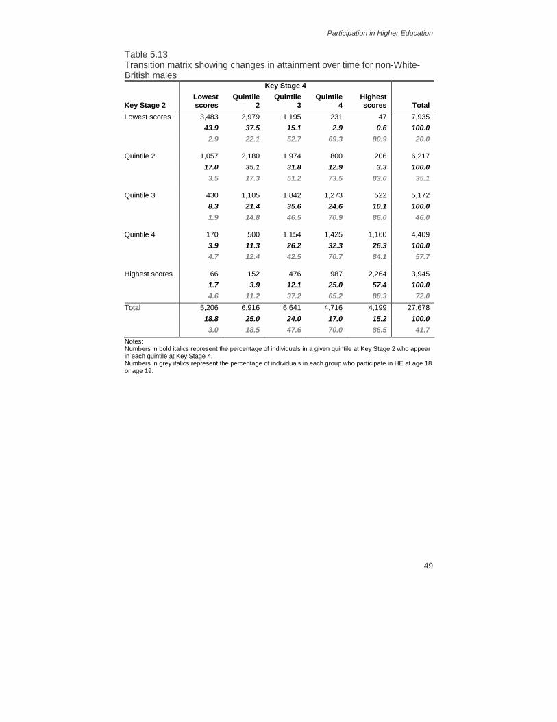
Participation in Higher Education
49
Table 5.13 Transition matrix showing changes in attainment over time for non-White-British males Key Stage 4
Key Stage 2 Lowest scores
Quintile 2
Quintile 3
Quintile 4
Highest scores Total
Lowest scores 3,483 2,979 1,195 231 47 7,935 43.9 37.5 15.1 2.9 0.6 100.0 2.9 22.1 52.7 69.3 80.9 20.0
Quintile 2 1,057 2,180 1,974 800 206 6,217 17.0 35.1 31.8 12.9 3.3 100.0 3.5 17.3 51.2 73.5 83.0 35.1
Quintile 3 430 1,105 1,842 1,273 522 5,172 8.3 21.4 35.6 24.6 10.1 100.0 1.9 14.8 46.5 70.9 86.0 46.0
Quintile 4 170 500 1,154 1,425 1,160 4,409 3.9 11.3 26.2 32.3 26.3 100.0 4.7 12.4 42.5 70.7 84.1 57.7
Highest scores 66 152 476 987 2,264 3,945 1.7 3.9 12.1 25.0 57.4 100.0 4.6 11.2 37.2 65.2 88.3 72.0 Total 5,206 6,916 6,641 4,716 4,199 27,678 18.8 25.0 24.0 17.0 15.2 100.0 3.0 18.5 47.6 70.0 86.5 41.7 Notes: Numbers in bold italics represent the percentage of individuals in a given quintile at Key Stage 2 who appear in each quintile at Key Stage 4. Numbers in grey italics represent the percentage of individuals in each group who participate in HE at age 18 or age 19.

Widening Participation in Higher Education
50
Table 5.14 Transition matrix showing changes in attainment over time for non-White-British females Key Stage 4
Key Stage 2 Lowest scores
Quintile 2
Quintile 3
Quintile 4
Highest scores Total
Lowest scores 2,170 2,960 1,756 476 91 7,453 29.1 39.7 23.6 6.4 1.2 100.0 4.2 17.6 48.1 69.5 84.6 25.0
Quintile 2 559 1,629 2,341 1,387 376 6,292 8.9 25.9 37.2 22.0 6.0 100.0 3.9 16.0 47.2 74.8 88.0 43.8
Quintile 3 224 687 1,691 1,795 1,062 5,459 4.1 12.6 31.0 32.9 19.5 100.0 2.7 13.7 43.4 72.3 87.9 56.1
Quintile 4 113 260 946 1,592 1,904 4,815 2.3 5.4 19.6 33.1 39.5 100.0 1.8 9.2 40.0 67.2 87.6 65.3
Highest scores 39 68 300 783 2,804 3,994 1.0 1.7 7.5 19.6 70.2 100.0 7.7 13.2 42.3 64.0 89.2 78.6 Total 3,105 5,604 7,034 6,033 6,237 28,013 11.1 20.0 25.1 21.5 22.3 100.0 4.0 16.2 45.3 70.2 88.3 49.9 Notes: Numbers in bold italics represent the percentage of individuals in a given quintile at Key Stage 2 who appear in each quintile at Key Stage 4. Numbers in grey italics represent the percentage of individuals in each group who participate in HE at age 18 or age 19.
5.4 Conclusions
This chapter has clearly demonstrated the importance of material deprivation, neighbourhood parental education and ethnic origin in determining HE participation rates at age 18 or 19. The raw differences between advantaged and disadvantaged students, and between different ethnic groups, are sizeable. Generally, disadvantaged students are significantly less likely to attend HE than more advantaged students, while many ethnic minority students are significantly more likely to participate in HE than their White British peers.
At least part of the large raw gap in HE participation rates between advantaged and disadvantaged students is attributable to the quality of schools (or quality of peers) accessed by poorer children. The role of school quality and its association with HE participation rates is complex, however, with interactions between school

Participation in Higher Education
51
quality, ethnicity and gender. In any case, this work cannot prove a causal link between the quality of secondary schooling accessed by a pupil and his or her academic achievement. We merely note that different types of students are accessing different types of schools and that this is likely to explain part of the story behind the large raw gaps in HE participation that we observe.
The key finding from this chapter, however, is that once we take into account the prior attainment of students, the large gaps in HE participation rates between different types of students are markedly reduced. For example, after allowing for prior achievement (from Key Stage 2 to Key Stage 5) plus a range of individual characteristics, the 20% most materially deprived males (females) are just 1.0 (2.1) percentage points less likely to participate in HE than their more advantaged counterparts. Equally, some of the apparent advantage of ethnic minority students is reduced once we take into account prior educational attainment. This means that some ethnic minority groups are more likely to participate in HE simply because they have higher achievement in secondary school. This pattern is not consistent at every stage though, because many ethnic minority groups make greater improvements in attainment between Key Stage 2 and Key Stage 4 than White British students. Thus, for example, before allowing for prior attainment, Black African males are 9.6 percentage points more likely to go to university than their White British male counterparts. After taking into account Key Stage 2 and Key Stage 3 attainment, this gap increases to 13.9 percentage points, but it falls back to 8.6 percentage points once we allow for prior attainment at GCSE and A level. This is one example of the way in which different groups of students experience very different academic trajectories as they progress through secondary school and on to higher education.
The richness of our analysis has illustrated that to widen participation in higher education to different groups of students, we need to pay closer attention to when gaps in educational achievement occur and how they develop during different phases of schooling. The analysis of transitions made by different students between Key Stage 2 and Key Stage 4 suggests that disadvantaged children who are low achievers when they enter secondary school are more likely to remain low achievers than more advantaged children. On the other hand, there is more upward mobility for most ethnic minority groups than for White British children. However, by and large it is reassuring that if more disadvantaged pupils do improve their educational performance between Key Stage 2 and Key Stage 4, they are at least as likely to participate in HE as their more advantaged counterparts (although the same cannot be said for White British students).

52
CHAPTER 6 Status of HE Institution Attended
In this chapter, we analyse the importance of the same three factors – material deprivation, neighbourhood parental education and ethnicity – for attending higher education institutions (HEIs) of different statuses. The impact of these characteristics on the status of universities attended by HE participants is clearly important, but there has been little quantitative analysis of this issue in the literature (see Gorard et al. (2006) for a summary). Clearly, an effective Widening Participation agenda ought to target disparities in participation not only in HE as a binary decision, but also across the spectrum of HE institutions, especially given evidence that returns to degrees vary according to institution type (Iftikhar, McNally and Telhaj, 2008).
In Section 6.1, we report raw differences in the status of HEI attended by material deprivation status, neighbourhood parental education and ethnicity, and show how these gaps change once school quality and other individual characteristics are included in the model. In Section 6.2, we go on to illustrate how these estimates are affected by the inclusion of educational attainment measures from Key Stage 2 (age 11) to Key Stage 5 (age 18). Section 6.3 offers some brief conclusions.
6.1 Baseline estimates of differences in status of HE institution attended
In this section, we first present raw estimates of the impact of material deprivation,44 neighbourhood parental education and ethnicity on the probability of attending a ‘high-status’ university for HE participants (see Chapter 2 for our definition of ‘high-status’ institutions). We then move on to see how these estimates change once we add measures of school quality and other individual-level characteristics to our model. The analysis is presented separately for males (Section 6.1.1) and females (Section 6.1.2).
6.1.1 Males Table 6.1 presents raw estimates (across schools) and estimates controlling for school quality (within schools) of the impact of material deprivation, neighbourhood parental education and ethnicity on the likelihood of going to a high-status HEI for boys who participate in higher education at age 18 or 19.
44 Estimates using FSM status alone as an indicator of material deprivation show broadly similar results. These results are available from the authors on request.
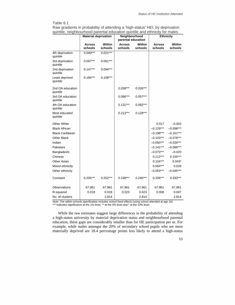
Status of HE Institution Attended
53
Table 6.1 Raw gradients in probability of attending a ‘high-status’ HEI, by deprivation quintile, neighbourhood parental education quintile and ethnicity for males Material deprivation Neighbourhood
parental education Ethnicity
Across schools
Within schools
Across schools
Within schools
Across schools
Within schools
4th deprivation quintile
0.040*** 0.021***
3rd deprivation quintile
0.097*** 0.061***
2nd deprivation quintile
0.147*** 0.094***
Least deprived quintile
0.184*** 0.108***
2nd OA education quintile
0.038*** 0.026***
3rd OA education quintile
0.086*** 0.057***
4th OA education quintile
0.131*** 0.082***
Most educated quintile
0.213*** 0.128***
Other White 0.017 –0.002 Black African –0.129*** –0.098*** Black Caribbean –0.198*** –0.161*** Other Black –0.103*** –0.078*** Indian –0.050*** –0.029*** Pakistani –0.141*** –0.086*** Bangladeshi –0.073*** –0.020 Chinese 0.112*** 0.100*** Other Asian 0.104*** 0.043* Mixed ethnicity 0.064*** 0.026 Other ethnicity –0.053*** –0.045***
Constant 0.205*** 0.252*** 0.198*** 0.246*** 0.336*** 0.333*** Observations 67,961 67,961 67,961 67,961 67,961 67,961 R-squared 0.018 0.018 0.023 0.023 0.008 0.007 No. of clusters 2,814 2,814 2,814 Note: The within-schools specification includes school fixed effects (using school attended at age 16). *** indicates significance at the 1% level, ** at the 5% level and * at the 10% level.
While the raw estimates suggest large differences in the probability of attending a high-status university by material deprivation status and neighbourhood parental education, these gaps are considerably smaller than for HE participation per se. For example, while males amongst the 20% of secondary school pupils who are most materially deprived are 18.4 percentage points less likely to attend a high-status

Widening Participation in Higher Education
54
university than males amongst the 20% of pupils who are least materially deprived (conditional on participation), they are 29.0 percentage points less likely to attend in the first place. Similarly, while males amongst the 20% of secondary school pupils from the least highly educated neighbourhoods are 21.3 percentage points less likely to attend a high-status HEI than males amongst the 20% of secondary school pupils from the most highly educated neighbourhoods (conditional on participation), they are 34.6 percentage points less likely to participate originally.
The raw estimates also reveal some striking differences by ethnic group: while male HE participants of Chinese, Other Asian and Mixed ethnic origin are significantly more likely to go to a high-status university than White British male participants, males of Black, Indian, Pakistani, Bangladeshi and Other ethnic origin are significantly less likely to do so. For Black African, Indian, Pakistani and Bangladeshi boys, this is in contrast to the findings for HE participation per se, in which they experienced a significant advantage relative to White British male students. (This is also true for girls from these ethnic groups – see Section 6.1.2.)
Table 6.1 also demonstrates the importance of school quality (the within-schools model) in determining the status of university attended (at age 18 or 19). In terms of material deprivation, the difference between the most deprived quintile and the least deprived quintile is reduced from 18.4 percentage points to 10.8 percentage points. Similarly, the difference between the 20% of boys from the best-educated neighbourhoods and the 20% of boys from the most poorly educated neighbourhoods falls from 21.3 percentage points to 12.8 percentage points. It thus appears that approximately 40% of the observed raw disparities are accounted for by differences in the quality of secondary school attended by different types of students (with those from the least materially deprived backgrounds and/or those from highly educated neighbourhoods typically going to better schools).45
The inclusion of controls for school quality tends to make a relatively smaller difference to the impact of ethnicity on the status of HEI attended. In all cases, the absolute value of the difference is reduced – so, for example, Pakistani male participants are now only 8.6 percentage points less likely to go to a high-status university than White British male participants (compared with 14.1 percentage points before the inclusion of controls for school quality), while Other Asian male participants are now only 4.3 percentage points more likely to go to a high-status university than White British male participants (compared with a raw difference of 10.4 percentage points). This suggests that ethnic minority boys experiencing a raw disadvantage (boys of Black, Indian, Pakistani, Bangladeshi and Other ethnic origin) go to relatively poorer schools than White British boys, while ethnic minority boys experiencing a raw advantage (boys of Chinese, Other Asian and Mixed ethnic origin) go to relatively better schools. This suggests a potentially fundamental role for schools in determining the status of HEI attended.
Table 6.2 moves on to include all three factors – material deprivation, neighbourhood parental education and ethnicity – in the same model, such that the impact of each characteristic is now conditional on the impacts of the other two.46
45 But see the discussion in Chapter 4 on the difficulties of fully identifying the effects of school quality in models such as ours. 46 The results presented in Table 6.2 also control for school quality (i.e. include school fixed effects).

Status of HE Institution Attended
55
Table 6.2 Gradients in probability of attending a ‘high-status’ HEI, controlling for individual-level characteristics (excluding prior attainment) for males Controlling for
deprivation, neighbourhood
parental educationand ethnicity
Plus other individual-level characteristics
4th deprivation quintile 0.004 0.003 3rd deprivation quintile 0.031*** 0.028*** 2nd deprivation quintile 0.052*** 0.049*** Least deprived quintile 0.055*** 0.052***
2nd OA education quintile 0.014* 0.015* 3rd OA education quintile 0.035*** 0.035*** 4th OA education quintile 0.055*** 0.054*** Most educated quintile 0.097*** 0.098***
Other White 0.000 0.002 Black African –0.079*** –0.073*** Black Caribbean –0.144*** –0.141*** Other Black –0.063** –0.057** Indian –0.021** –0.016 Pakistani –0.067*** –0.058*** Bangladeshi 0.000 0.007 Chinese 0.108*** 0.114*** Other Asian 0.052** 0.054** Mixed ethnicity 0.033* 0.032* Other ethnicity –0.032** –0.027*
Constant 0.237*** 0.254*** Observations 67,961 67,961 R-squared 0.032 0.036 No. of clusters 2,814 2,814 F-test of additional controls (p-value) 0 0 Notes: All models include school fixed effects (on the basis of school attended at age 16). In addition to deprivation quintile, neighbourhood parental education quintile and ethnicity, column 2 also includes controls for month of birth, whether English is the pupil’s first language and whether they have either statemented (more severe) or non-statemented (less severe) special educational needs (measured at age 16). *** indicates significance at the 1% level, ** at the 5% level and * at the 10% level.
To the extent that materially deprived students tend to come from poorly educated neighbourhoods (and ethnic minority students tend to be more materially deprived and to come from less well-educated neighbourhoods), we would expect the inclusion of all three factors in the same model to reduce the magnitude of the impact of each characteristic individually.

Widening Participation in Higher Education
56
This expectation is borne out by the results shown in Table 6.2. For example, the impact (for male participants) of being amongst the 20% least materially deprived pupils (compared with the 20% most materially deprived pupils) on the likelihood of going to a high-status university at age 18 or 19 approximately halves once we control for neighbourhood parental education and ethnicity – from 10.8 percentage points to 5.5 percentage points. Whilst the effects on the estimates of neighbourhood parental education and ethnicity are somewhat smaller, the inclusion of additional controls still makes a difference in most cases: for example, the advantage (in terms of the likelihood of attending a high-status HEI) of male participants from the most highly educated neighbourhoods falls from 12.8 percentage points to 9.7 percentage points; similarly, the disadvantage faced by males of Black African ethnic origin (compared with males of White British ethnic origin) falls from 9.8 percentage points to 7.9 percentage points.
The second column of Table 6.2 further controls for month of birth, whether English is the pupil’s first language and whether they have special educational needs (measured at age 16). In most cases, the inclusion of these characteristics makes very little difference to the estimated effects of material deprivation, neighbourhood parental education and ethnicity on the likelihood of attending a high-status university at age 18 or 19 amongst HE participants; this is in contrast to the results for HE participation per se (discussed in Section 5.1), for which the inclusion of these characteristics made a sizeable difference in some cases. For example, amongst males of Black African ethnic origin, the inclusion of these additional controls reduces the advantage they have over White British males in terms of HE participation from 13.3 to 9.6 percentage points, while it reduces the disadvantage they face in terms of attending a high-status HEI by only 0.6 (7.9 to 7.3) percentage points.
6.1.2 Females Table 6.3 presents our raw (across schools) and baseline (within schools) estimates of the impact of material deprivation, neighbourhood parental education and ethnicity on the likelihood of attending a high-status HEI at age 18 or 19 for female HE participants.
As was the case for males, the raw estimates of the effect of material deprivation and neighbourhood parental education on the likelihood of going to a high-status university are large and significant for female HE participants (albeit smaller than for participation at any HEI – see Table 5.3 in Section 5.1.2 for details). For example, female participants amongst the 20% of secondary school pupils who are least materially deprived are 19.1 percentage points more likely (than female participants amongst the 20% of pupils who are most materially deprived) to attend a high-status HEI at age 18 or 19. Similarly, females amongst the 20% of pupils from the most highly educated neighbourhoods are 23.9 percentage points more likely to attend a high-status university than females amongst the 20% of pupils from the least well-educated neighbourhoods.
A similar pattern to that found for males is also evident in terms of the impact of ethnicity on the likelihood of attending a good university, with females of Chinese, Other Asian or Mixed ethnic origin significantly more likely – and females of

Status of HE Institution Attended
57
Table 6.3 Raw gradients in probability of attending a ‘high-status’ HEI, by deprivation quintile, neighbourhood parental education quintile and ethnicity for females Material deprivation Neighbourhood
parental education Ethnicity
Across schools
Within schools
Across schools
Within schools
Across schools
Within schools
4th deprivation quintile
0.033*** 0.027***
3rd deprivation quintile
0.083*** 0.057***
2nd deprivation quintile
0.137*** 0.095***
Least deprived quintile
0.191*** 0.121***
2nd OA education quintile
0.046*** 0.028***
3rd OA education quintile
0.087*** 0.056***
4th OA education quintile
0.142*** 0.089***
Most educated quintile
0.239*** 0.144***
Other White 0.050*** 0.014 Black African –0.084*** –0.054*** Black Caribbean –0.149*** –0.114*** Other Black –0.113*** –0.087*** Indian –0.053*** –0.016 Pakistani –0.100*** –0.063*** Bangladeshi –0.089*** –0.044** Chinese 0.135*** 0.117*** Other Asian 0.115*** 0.054** Mixed ethnicity 0.090*** 0.037** Other ethnicity –0.003 0.002
Constant 0.206*** 0.244*** 0.184*** 0.236*** 0.326*** 0.324*** Observations 85,260 85,260 85,260 85,260 85,260 85,260 R-squared 0.021 0.020 0.030 0.030 0.006 0.006 No. of clusters 2,852 2,852 2,852 Note: The within-schools specification includes school fixed effects (using school attended at age 16). *** indicates significance at the 1% level, ** at the 5% level and * at the 10% level.
Black, Indian, Pakistani or Bangladeshi ethnic origin significantly less likely – to attend a high-status HEI than females of White British ethnic origin. There are some interesting differences to note (compared with the findings for boys). First, while females of Other White ethnic origin are 5.0 percentage points significantly more likely to attend a high-status university than females of White British ethnic origin,

Widening Participation in Higher Education
58
the difference observed for Other White males is positive but insignificant. Second, while males of Other ethnic origin are 5.3 percentage points significantly less likely to attend a high-status university than White British males, the raw effect for females of Other ethnic origin is negative but insignificant.
The inclusion of controls for school quality (the within-schools model) has an effect on estimates of the impact of material deprivation, neighbourhood parental Table 6.4 Gradients in probability of attending a ‘high-status’ HEI, controlling for individual-level characteristics (excluding prior attainment) for females Controlling for
deprivation, neighbourhood
parental educationand ethnicity
Plus other individual-level characteristics
4th deprivation quintile 0.011* 0.009 3rd deprivation quintile 0.028*** 0.025*** 2nd deprivation quintile 0.053*** 0.050*** Least deprived quintile 0.065*** 0.062***
2nd OA education quintile 0.016** 0.016** 3rd OA education quintile 0.036*** 0.036*** 4th OA education quintile 0.061*** 0.062*** Most educated quintile 0.111*** 0.111***
Other White 0.018 0.022* Black African –0.033** –0.025* Black Caribbean –0.093*** –0.093*** Other Black –0.068*** –0.065*** Indian –0.008 0.002 Pakistani –0.045*** –0.033** Bangladeshi –0.022 –0.009 Chinese 0.126*** 0.137*** Other Asian 0.067*** 0.075*** Mixed ethnicity 0.047*** 0.048*** Other ethnicity 0.016 0.022
Constant 0.221*** 0.231*** Observations 85,260 85,260 R-squared 0.039 0.041 No. of clusters 2,852 2,852 F-test of additional controls (p-value) 0 0 Notes: All models include school fixed effects (on the basis of school attended at age 16). In addition to deprivation quintile, neighbourhood parental education quintile and ethnicity, column 2 also includes controls for month of birth, whether English is the pupil’s first language and whether they have either statemented (more severe) or non-statemented (less severe) special educational needs (measured at age 16). *** indicates significance at the 1% level, ** at the 5% level and * at the 10% level.

Status of HE Institution Attended
59
education and ethnicity for female participants similar to the effect for male participants. For example, the advantage (in terms of status of HEI attended) of being a female in the least materially deprived quintile (relative to the most materially deprived quintile) falls from 19.1 to 12.1 percentage points; similarly, it falls from 23.9 to 14.4 percentage points for females amongst the 20% of pupils from the best-educated neighbourhoods (compared with those amongst the 20% of pupils from the most poorly educated neighbourhoods).
The first column of Table 6.4 shows how these within-school estimates change once we include material deprivation, neighbourhood parental education and ethnicity in the same model. Conditional on neighbourhood parental education and ethnicity (and school quality), female HE participants amongst the 20% of secondary school pupils experiencing the lowest material deprivation are 6.5 percentage points more likely to attend a high-status university than female participants amongst the 20% of pupils experiencing the greatest material deprivation; this is a reduction of around 45% compared with controlling for material deprivation and school quality alone. Similarly, the impact of being amongst the 20% of pupils from the best-educated neighbourhoods (compared with being amongst the 20% of pupils from the most poorly educated neighbourhoods) falls from 14.4 percentage points to 11.1 percentage points once we account for material deprivation and ethnicity, while the coefficients on most ethnic groups change relatively little. In all cases, these effects are of approximately similar magnitude to – and go in the same direction as – those found for boys.
Again as was the case for boys, the inclusion of controls for month of birth, English as an additional language and special educational needs (shown in the second column of Table 6.4) makes little difference to our estimates of the effect of material deprivation, neighbourhood parental education and ethnicity on the likelihood of attending a high-status university, suggesting that these characteristics are more likely to affect HE participation (at age 18 or 19) per se rather than the status of institution attended (conditional on participation at age 18 or 19).
6.2 The role of prior attainment in the HE status gradient
Up to now, one of the potentially key determinants of the status of HE institution attended – prior attainment – has been omitted from the analysis. To the extent that participation decisions at age 18 or 19 are the result of previous schooling decisions and outcomes, disparities in the types of universities attended by pupils according to material deprivation status, neighbourhood parental education levels and ethnicity may potentially be traced back to differences in earlier academic outcomes for these individuals. In this section, we exploit the retrospective information available to us and sequentially consider the impact of test scores from age 11 to age 18 on the estimated effects of material deprivation, neighbourhood parental education and ethnicity on the likelihood of going to a high-status university at age 18 or 19. We do this separately for males (in Section 6.2.1) and females (in Section 6.2.2).

Widening Participation in Higher Education
60
6.2.1 Males The first column of Table 6.5 replicates the results found in column 2 of Table 6.2, i.e. it shows the impact of material deprivation, neighbourhood parental education and ethnicity on the likelihood of attending a high-status university for HE participants, controlling for school quality, month of birth, whether English is the student’s first language and whether they have special educational needs. Columns 2 through 5 illustrate how these estimates change once we include test results from Key Stage 2 (age 11), Key Stage 3 (age 14), Key Stage 4 (age 16) and Key Stage 5 (age 18) respectively.
We see from Table 6.5 that the inclusion of prior educational attainment significantly reduces the impact of material deprivation status and neighbourhood parental education levels on the status of HE institution attended by male participants. The inclusion of Key Stage 2 and Key Stage 3 results reduces, but does not eliminate, the penalty faced by boys amongst the 20% of secondary school pupils facing the greatest material deprivation and boys amongst the 20% of pupils from the most poorly educated neighbourhoods. However, the inclusion of Key Stage 4 (GCSE and equivalent) results has a greater impact on material deprivation than it does on neighbourhood parental education: while material deprivation status no longer affects the probability of attending a high-status university, neighbourhood parental education does – at least for males amongst the 20% of pupils from the most poorly educated neighbourhoods vis-à-vis males amongst the 40% of pupils from the most highly educated neighbourhoods. This is an interesting finding, and provides some evidence to suggest that highly educated parents may be better-equipped to help their children apply for the top universities than less highly educated parents. (Of course, it must be remembered that we do not have individual-level measures of parental education, but are using a proxy measure based on neighbourhood characteristics instead.) Indeed, these differences according to neighbourhood parental education levels persist even after Key Stage 5 results are taken into account – with male participants from the most highly educated neighbourhoods being 3.0 percentage points more likely to attend a high-status university at age 18 or 19 than boys from more poorly educated neighbourhoods.
The inclusion of controls for prior attainment is particularly important in understanding the influence of ethnicity on the probability of attending a high-status HE institution (conditional on participation at age 18 or 19). For example, once we include Key Stage 2 results in our model, male participants of Indian and Bangladeshi ethnic origin go from being as likely as White British males to attend a high-status university at age 18 or 19 to being significantly more likely to do so; on the other hand, boys of Other Black, Pakistani and Other ethnic origin go from being significantly less likely to attend a high-status HEI to being equally likely to do so, compared with White British males. This suggests that if boys from these ethnic groups can achieve the same outcomes at Key Stage 2 as White British boys with the same observable characteristics, then they will have significantly improved their chances of attending a high-status university (conditional on attending HE participation at age 18 or 19). This is an important finding in terms of the Widening Participation agenda.

Status of HE Institution Attended
61
Table 6.5 Gradients in status of HEI attended by males, controlling for individual-level characteristics and prior attainment Individual-
level controls
Plus Key Stage 2 results
Plus Key Stage 3 results
Plus Key Stage 4 results
Plus Key Stage 5 results
4th deprivation quintile 0.003 –0.002 –0.004 –0.007 –0.007 3rd deprivation quintile 0.028*** 0.016** 0.010 –0.001 –0.004 2nd deprivation quintile 0.049*** 0.033*** 0.022*** 0.008 0.004 Least deprived quintile 0.052*** 0.034*** 0.021** 0.005 –0.002
2nd OA education quintile 0.015* 0.011 0.006 –0.001 –0.005 3rd OA education quintile 0.035*** 0.029*** 0.020** 0.011 0.002 4th OA education quintile 0.054*** 0.042*** 0.033*** 0.018** 0.008 Most educated quintile 0.098*** 0.082*** 0.068*** 0.046*** 0.030***
Other White 0.002 0.017 0.015 0.012 0.008 Black African –0.073*** –0.031* –0.012 –0.002 0.000 Black Caribbean –0.141*** –0.090*** –0.053*** –0.035** –0.019 Other Black –0.057** –0.007 0.013 0.028 0.029 Indian –0.016 0.036*** 0.037*** 0.025** 0.024** Pakistani –0.058*** 0.003 0.018 0.014 0.019 Bangladeshi 0.007 0.048** 0.045** 0.033 0.044** Chinese 0.114*** 0.126*** 0.106*** 0.090*** 0.076*** Other Asian 0.054** 0.074*** 0.059** 0.039* 0.031 Mixed ethnicity 0.032* 0.033* 0.027 0.016 0.020 Other ethnicity –0.027* 0.002 0.008 0.006 0.016
Constant 0.254*** 0.056*** –0.002 0.032* –0.018 Observations 67,961 67,961 67,961 67,961 67,961 R-squared 0.036 0.128 0.191 0.277 0.391 No. of clusters 2,814 2,814 2,814 2,814 2,814 F-test of additional controls (p-value)
0 0 0 0 0
Notes: The results presented in column 1 replicate those found in column 2 of Table 6.2. All models are within-school (i.e. we include school fixed effects on the basis of school attended at age 16). *** indicates significance at the 1% level, ** at the 5% level and * at the 10% level.
Where differences across ethnicity remain significant (following the inclusion of Key Stage 2 results), the successive inclusion of Key Stage 3, Key Stage 4 and Key Stage 5 results serves to reduce the advantage (or disadvantage, in the case of Black Caribbean boys) that ethnic minority boys exhibit over White British boys in terms of the likelihood of going to a high-status university. For example, while Other Asian males are 7.4 percentage points more likely (and Black Caribbean males 9.0 percentage points less likely) than White British males to attend a high-status HEI after controlling for Key Stage 2 results, they are all just as likely to do so following the inclusion of test results from Key Stage 3 to Key Stage 5.

Widening Participation in Higher Education
62
Even once we have taken into account prior educational attainment from age 11 to age 18, however, male participants of Indian, Bangladeshi and Chinese ethnic origin are still significantly more likely to attend a high-status HEI than males of White British ethnic origin. As for HE participation, therefore, a Widening Participation agenda may need to be concerned about improving the outcomes of White British boys.
6.2.2 Females The first column of Table 6.6 presents estimates (for females) of the impact of material deprivation, neighbourhood parental education and ethnicity on the likelihood of attending a high-status university, controlling for school quality, month of birth, whether English is the student’s first language and whether they have special educational needs.47 In columns 2 through 5, we build up our model by sequentially adding academic attainment from Key Stage 2 (age 11) to Key Stage 5 (age 18).
The inclusion of prior educational attainment monotonically reduces the impacts of material deprivation and neighbourhood parental education on the likelihood of attending a high-status university (conditional on participation at age 18 or 19) for females. For example, controlling for schooling attainment reduces the advantage associated with being a girl amongst the 20% of pupils experiencing the least material deprivation (compared with being a girl amongst the 20% of pupils experiencing the most material deprivation) from 6.2 to 4.4 percentage points (Key Stage 2), 2.8 percentage points (Key Stage 3) and 1.2 percentage points (Key Stage 4), before becoming insignificant following the inclusion of Key Stage 5 results.
By contrast, as was the case for boys, the impact of neighbourhood parental education on the probability of attending a high-status institution remains positive and significant even after controlling for A-level (or equivalent) outcomes. For example, female participants amongst the 20% of pupils from the most well-educated neighbourhoods remain 4.0 percentage points more likely to attend a high-status university than female participants amongst the 20% of pupils from the least well-educated neighbourhoods even after we include test results from Key Stage 2 to Key Stage 5. This suggests both that the impact of neighbourhood parental education on the probability of attending a high-status HEI is greater than the impact of material deprivation on the same outcome, and that the impact of neighbourhood parental education is greater for females than it is for males (for whom the difference was only 3.0 percentage points).
47 This replicates the second column of Table 6.4.

Status of HE Institution Attended
63
Table 6.6 Gradients in status of HEI attended by females, controlling for individual-level characteristics and prior attainment Individual-
level controls
Plus Key Stage 2 results
Plus Key Stage 3 results
Plus Key Stage 4 results
Plus Key Stage 5 results
4th deprivation quintile 0.009 0.003 –0.003 –0.007 –0.007 3rd deprivation quintile 0.025*** 0.016** 0.005 –0.005 –0.007 2nd deprivation quintile 0.050*** 0.037*** 0.024*** 0.011* 0.009 Least deprived quintile 0.062*** 0.044*** 0.028*** 0.012* 0.008
2nd OA education quintile 0.016** 0.010 0.007 0.002 0.001 3rd OA education quintile 0.036*** 0.025*** 0.019*** 0.010* 0.005 4th OA education quintile 0.062*** 0.047*** 0.038*** 0.027*** 0.017*** Most educated quintile 0.111*** 0.091*** 0.077*** 0.060*** 0.040***
Other White 0.022* 0.035*** 0.039*** 0.030*** 0.020** Black African –0.025* 0.005 0.019 0.024* 0.018 Black Caribbean –0.093*** –0.039*** –0.020 –0.012 –0.010 Other Black –0.065*** –0.024 –0.007 –0.002 0.003 Indian 0.002 0.046*** 0.041*** 0.031*** 0.039*** Pakistani –0.033** 0.026** 0.039*** 0.029** 0.042*** Bangladeshi –0.009 0.042** 0.044** 0.027 0.031* Chinese 0.137*** 0.153*** 0.125*** 0.105*** 0.097*** Other Asian 0.075*** 0.101*** 0.080*** 0.063*** 0.074*** Mixed ethnicity 0.048*** 0.045*** 0.036** 0.032** 0.029** Other ethnicity 0.022 0.045*** 0.047*** 0.044*** 0.045***
Constant 0.231*** 0.047*** 0.014 0.019 0.001 Observations 85,260 85,260 85,260 85,260 85,260 R-squared 0.041 0.120 0.170 0.217 0.315 No. of clusters 2,852 2,852 2,852 2,852 2,852 F-test of additional controls (p-value)
0 0 0 0 0
Notes: The results presented in column 1 replicate those found in column 2 of Table 6.4. All models are within-school (i.e. we include school fixed effects on the basis of school attended at age 16). *** indicates significance at the 1% level, ** at the 5% level and * at the 10% level.
The inclusion of Key Stage 2 results reduces the penalty faced by Black Caribbean girls, increases the advantage faced by girls of Chinese and Other Asian ethnic origin, eliminates the disadvantage faced by girls of Black African and Other Black ethnic origin and turns a disadvantage into an advantage for Pakistani girls in terms of the probability of attending a high-status university at age 18 or 19 relative to White British girls. Thereafter, the inclusion of Key Stage 3, Key Stage 4 and Key Stage 5 results generally reduces – but does not eliminate – the impact of ethnicity on the likelihood of attending a high-status university (exceptions are for Black Caribbean girls, the effect on whom becomes insignificant, and for Pakistani

Widening Participation in Higher Education
64
girls, whose advantage grows). Indeed, using our final model specification, females of Other White, Indian, Pakistani, Bangladeshi, Chinese, Other Asian, Mixed and Other ethnic origin are all still significantly more likely to attend a high-status HEI than female participants of White British ethnic origin, suggesting that ethnicity plays a greater role for females than it does for males in determining this outcome.
6.3 Conclusions
This chapter has shown that the Widening Participation agenda should not only be concerned about participation in higher education per se, but also about the status of institutions attended by participants from different backgrounds. While the impact of material deprivation on the likelihood of attending a high-status university disappears once we include Key Stage 5 outcomes, the effects of neighbourhood parental education remain significant. This suggests that young people from well-educated neighbourhoods are better able to secure places in high-status universities. Given that we do not have individual-level data on parental education, we cannot say much more than this, although we could speculate that better-educated parents may be better able to assist their children in accessing higher-status HEIs either directly (through alumni networks, for example) or indirectly (by accessing better schools, for example).
In contrast to the findings for HE participation (discussed in Chapter 5), the raw results for many ethnic minority groups suggest that they are significantly less likely to attend a high-status university at age 18 or 19 than White British students. However, our final specification suggests that this disadvantage arises largely from differences in other characteristics – particularly prior educational attainment – because once we control for such factors, the estimated effects become either positive and significant, or insignificant – mirroring the findings for HE participation (see Section 5.2 for details). Once we control for prior attainment, Indian, Bangladeshi and Chinese males are more likely to attend a high-status HE institution than White British males, while females of Other White, Indian, Pakistani, Bangladeshi, Chinese, Other Asian, Mixed and Other ethnic origin are all significantly more likely to attend a high-status university than White British females.
65
CHAPTER 7 Subject Choice
In this chapter, we analyse HE participants’ choice of degree subject. This is important because, as noted earlier, different degree subjects yield different rates of return in the labour market (Walker and Zhu, 2005; Iftikhar, McNally and Telhaj, 2008). This may be of concern if, for example, there is little in the way of a socio-economic gap in overall HE participation conditional on prior achievement (as shown in Chapter 5) but poorer students generally access the types of degree subjects that yield lower economic value in the labour market. We focus on a number of different specific subjects and subject groupings. In Section 7.1, we consider access to Science, Technology, Engineering and Mathematics degrees (STEM subjects – see Section 3.3 for full details). These are generally (but not universally) subjects that yield high wage returns. In any case, they are certainly subjects in which the government has expressed a particular interest in increasing supply, so it is important to consider whether certain types of students are less likely to access such subjects. In Section 7.2, we focus on a specific high-return degree (Law) to illustrate differences across particular subjects of interest.48 Lastly, we make use of research from another strand of our ESRC-TLRP project (Iftikhar, McNally and Telhaj, 2008), which has been investigating returns to different degree subjects. We use this information in Section 7.3 to get a better understanding of the extent to which different types of student access higher-rewarding degree subjects. Section 7.4 offers some brief conclusions.
7.1 STEM subjects
We start by examining the determinants of taking a STEM degree subject for HE participants at age 18 and 19. The dependent variable therefore takes the value 1 if the individual is enrolled in a STEM subject and 0 if the individual is enrolled in HE in an alternative subject. We analyse males and females separately.
7.1.1 Males Table 7.1 presents baseline results which show the raw relationship between material deprivation, neighbourhood parental education and ethnicity and the likelihood of being enrolled in a STEM subject for males. We show, similarly to the results in Chapters 5 and 6, estimates both with and without school fixed effects.
As might be expected from the descriptive statistics outlined in Section 3.3.1, material deprivation is not correlated with being enrolled in a STEM subject amongst males. Interestingly, however, boys living in areas with the highest education levels are slightly less likely to enrol in a STEM subject at university than
48 Results for Mathematics and Medicine can be found in Appendices D and E of this report respectively.

Widening Participation in Higher Education
66
boys living in areas with the lowest education levels. This effect is reduced slightly (from 4.2 to 2.1 percentage points) once we compare students attending the same schools.
Table 7.1 Raw gradients in probability of studying a STEM subject at university, by deprivation quintile, neighbourhood parental education quintile and ethnicity for males Material deprivation Neighbourhood
parental education Ethnicity
Across schools
Within schools
Across schools
Within schools
Across schools
Within schools
4th deprivation quintile
0.002 0.009
3rd deprivation quintile
–0.002 0.005
2nd deprivation quintile
0.005 0.011
Least deprived quintile
–0.009 0.007
2nd OA education quintile
–0.014 –0.009
3rd OA education quintile
–0.016* –0.013
4th OA education quintile
–0.018** –0.009
Most educated quintile
–0.042*** –0.021**
Other White –0.020* –0.008 Black African –0.034** –0.040** Black Caribbean –0.056*** –0.050** Other Black –0.036 –0.031 Indian –0.024** –0.023** Pakistani –0.017 –0.026* Bangladeshi 0.003 –0.008 Chinese 0.107*** 0.109*** Other Asian –0.013 –0.002 Mixed ethnicity –0.034* –0.012 Other ethnicity 0.007 0.008
Constant 0.386*** 0.377*** 0.408*** 0.398*** 0.388*** 0.387*** Observations 67,961 67,961 67,961 67,961 67,961 67,961 R-squared 0 0 0.001 0.001 0.001 0.001 No. of clusters 2,814 2,814 2,814 Note: The within-schools specification includes school fixed effects (using school attended at age 16). *** indicates significance at the 1% level, ** at the 5% level and * at the 10% level.

Subject Choice
67
Table 7.2 Gradients in probability of studying a STEM subject at university, controlling for individual-level characteristics (excluding prior attainment) for males Controlling for
deprivation, neighbourhood
parental educationand ethnicity
Plus other individual-level characteristics
4th deprivation quintile 0.011 0.011 3rd deprivation quintile 0.008 0.009 2nd deprivation quintile 0.016 0.017* Least deprived quintile 0.014 0.015
2nd OA education quintile –0.012 –0.012 3rd OA education quintile –0.017* –0.017* 4th OA education quintile –0.014 –0.015 Most educated quintile –0.027** –0.027***
Other White –0.007 –0.013 Black African –0.038** –0.048** Black Caribbean –0.049** –0.048** Other Black –0.031 –0.035 Indian –0.023** –0.040*** Pakistani –0.024* –0.043*** Bangladeshi –0.007 –0.026 Chinese 0.110*** 0.093*** Other Asian –0.001 –0.013 Mixed ethnicity –0.012 –0.014 Other ethnicity 0.009 –0.003
Constant 0.393*** 0.381*** Observations 67,961 67,961 R-squared 0.001 0.002 No. of clusters 2,814 2,814 F-test of additional controls (p-value) 0 0 Notes: All models include school fixed effects (on the basis of school attended at age 16). In addition to deprivation quintile, neighbourhood parental education quintile and ethnicity, column 2 also includes controls for month of birth, whether English is the pupil’s first language and whether they have either statemented (more severe) or non-statemented (less severe) special educational needs (measured at age 16). *** indicates significance at the 1% level, ** at the 5% level and * at the 10% level.
Ethnicity, even taking into account school fixed effects, is more strongly correlated with enrolment in a STEM subject amongst boys. Specifically, Black Caribbean, Black African and Indian students are all significantly less likely (than White British students) to enrol in a STEM subject at university, while Chinese students are just under 11 percentage points more likely to enrol on a STEM course;

Widening Participation in Higher Education
68
these differences persist even after accounting for the schools attended by these pupils at age 16.
Table 7.2 shows how these results change once we control for material deprivation, neighbourhood parental education and ethnicity in the same model (column 1) and once we add other individual-level characteristics, i.e. month of birth, whether the student has English as an additional language and whether they have special educational needs. Table 7.2 does not control for prior achievement.
The results in Table 7.2 are broadly similar to those shown in Table 7.1, in that neither material deprivation nor neighbourhood parental education is strongly correlated with enrolment in a STEM subject. In terms of ethnicity, Black Caribbean, Black African, Indian and now Pakistani students are significantly less likely to take a STEM subject, after controlling for individual characteristics, while Chinese students are still more likely to do so (than White British boys).
We next add measures of prior achievement to the model sequentially. Columns 1 to 4 of Table 7.3 follow Chapters 5 and 6 by exploring the extent to which differences in the likelihood of enrolling in a STEM subject remain once we allow for Key Stage 2 to Key Stage 5 results. The table confirms that, even after allowing for prior achievement, material deprivation is not significantly associated with taking a STEM subject: individuals from the most deprived backgrounds are no more or less likely to enrol in a STEM subject than individuals from the least deprived backgrounds, given that they participate in HE in the first place. There is some evidence that individuals from neighbourhoods with higher levels of parental education are actually slightly less likely (by up to 3.3 percentage points) to enrol in a STEM subject, again conditional on their prior achievement. Adding Key Stage prior achievement measures from age 11 to age 18 reduces the number of ethnic minority groups that are significantly less likely (than White British males) to enrol in a STEM subject: only Indian males remain significantly less likely to do so (at conventional levels). This suggests that it was the poorer achievement of Black African and Black Caribbean boys that was driving their lower enrolment in STEM subjects. Chinese students, by contrast, remain significantly more likely to take a STEM degree subject, even after we control for their prior achievement.
One might argue, however, that controlling for pupils’ overall level of prior achievement is not sufficient. To enrol in Engineering at degree level, for example, it would be necessary for a student to have a minimum level of Mathematics at A level. Thus some of the reason students do not enrol in STEM subjects at degree level may simply be that they do not have the necessary academic preparation. We want to explore this issue in our modelling. Therefore, in the final column of Table 7.3, we add in an additional indicator of whether or not the student studied a STEM subject at A level.49 What is striking is that when we control for taking a STEM subject at A level, the ethnic gaps in the likelihood of enrolling in a STEM subject change substantially. Boys from almost every ethnic minority group (with the exception of Chinese, Other White and Other Black boys) become significantly less
49 We count passes (Grades A to E) in the following General A-level subjects in our definition of obtaining a STEM A level: Biology, Human Biology, Chemistry, Physics, Science (Single Award), Electronics, Environmental Science, Geology, Psychology, Maths, Mechanics, Pure Maths, Discrete Maths, Applied Maths, Statistics, Further Maths, Additional Maths, Computer Studies and IT. We also include passes in Vocational A levels (Single and Double Award) in Science, Engineering and ICT.

Subject Choice
69
Table 7.3 Gradients in probability of studying a STEM subject at university, controlling for individual-level characteristics and prior attainment for males Plus Key
Stage 2 results
Plus Key Stage 3 results
Plus Key Stage 4 results
Plus Key Stage 5 results
Plus STEM
A-level indicator
4th deprivation quintile 0.010 0.010 0.009 0.009 0.007 3rd deprivation quintile 0.006 0.004 0.003 0.005 0.004 2nd deprivation quintile 0.013 0.010 0.009 0.010 0.007 Least deprived quintile 0.011 0.007 0.006 0.007 0.003
2nd OA education quintile –0.013 –0.014 –0.015 –0.015 –0.013 3rd OA education quintile –0.019* –0.021** –0.022** –0.020** –0.015* 4th OA education quintile –0.017* –0.020** –0.022** –0.019* –0.015 Most educated quintile –0.031*** –0.035*** –0.037*** –0.033*** –0.025***
Other White –0.010 –0.010 –0.010 –0.012 –0.017 Black African –0.038* –0.032* –0.032 –0.033* –0.066*** Black Caribbean –0.036* –0.026 –0.025 –0.031 –0.046** Other Black –0.023 –0.017 –0.016 –0.018 –0.029 Indian –0.028** –0.027** –0.030** –0.029** –0.082*** Pakistani –0.029* –0.025 –0.026 –0.028 –0.069*** Bangladeshi –0.016 –0.017 –0.019 –0.019 –0.059** Chinese 0.096*** 0.090*** 0.089*** 0.089*** 0.023 Other Asian –0.008 –0.012 –0.014 –0.012 –0.074*** Mixed ethnicity –0.014 –0.015 –0.016 –0.016 –0.034* Other ethnicity 0.004 0.006 0.006 0.004 –0.028*
Constant 0.333*** 0.317*** 0.271*** 0.252*** 0.188*** Observations 67,961 67,961 67,961 67,961 67,961 R-squared 0.005 0.007 0.008 0.017 0.126 No. of clusters 2,814 2,814 2,814 2,814 2,814 F-test of additional controls (p-value)
0 0 0 0 0
Note: All models are within-school (i.e. we include school fixed effects on the basis of school attended at age 16). *** indicates significance at the 1% level, ** at the 5% level and * at the 10% level.
likely to take a STEM subject than White British boys, and Chinese students are now no more likely to enrol in a STEM degree than White British students, once we allow for STEM subjects at A level. In other words, this means that Chinese boys are more likely to take STEM subjects at A level than White British boys, and that this explains the gap in HE enrolment in STEM degree subjects that we observed in the previous column of Table 7.3. Once we allow for their higher probability of taking a STEM A level, Chinese students are no more likely to enrol in a STEM degree than similarly qualified White British students. By contrast, for other ethnic minority groups, when we allow for whether or not students study STEM subjects at

Widening Participation in Higher Education
70
A level, they become even less likely to study a STEM degree relative to White British students. This implies that these ethnic minority groups, with a given level of prior achievement, are genuinely less likely to study a STEM degree subject than White British students, which may be an issue of policy concern.
7.1.2 Females Table 7.4 shows the basic correlations between material deprivation, neighbourhood parental education levels and ethnicity and the likelihood of taking a STEM degree subject for females. Unlike for males, material deprivation is significantly correlated with the likelihood of taking a STEM degree subject: for example, females in the least deprived quintile are 1.9 percentage points more likely to study a STEM degree subject than females in the most deprived quintile, before allowing for school fixed effects. Thus the correlations, whilst significant, are not huge. Interestingly, neighbourhood parental education has a significant positive effect for girls, while it had a significant negative effect for boys: this suggests that (neighbourhood) parental education plays a differential role for males and females in terms of their likelihood of enrolling on a STEM course at university (conditional on HE participation). As was the case for males, females from some ethnic minority groups are significantly less likely to take a STEM subject: in particular, girls of Other White, Black Caribbean, Black African and Other Black ethnic origin. In all cases, the introduction of school fixed effects makes very little difference to these estimates, suggesting that differences in the types of schools attended by different pupils are not the driving force behind these raw disparities.
The first column of Table 7.5 moves on to include material deprivation, neighbourhood parental education and ethnicity in the same model, while the second column also adds other individual-level characteristics. The first shows that the results for material deprivation and neighbourhood parental education change markedly once we include all three characteristics of interest in the same model. Material deprivation and neighbourhood parental education are, by and large, no longer significantly correlated with the probability of a female enrolling in a STEM subject at university. In other words, much of the apparent correlation between material deprivation and the likelihood of studying a STEM subject (for example) can be explained by the correlation between neighbourhood parental education and ethnicity and the likelihood of enrolling in a STEM degree. In all cases, the inclusion of other individual characteristics does little to further alter the coefficients.
Lastly, Table 7.6 shows the results controlling for prior achievement. After allowing for prior achievement and whether the female took a STEM subject at A level, it is clear that material deprivation and neighbourhood parental education levels are not significantly related to the likelihood of enrolling in a STEM subject (at least not at conventional levels). This means that more deprived females are no more (or less) likely to take a STEM subject at university than their more advantaged counterparts, as was also generally the case for males. However, ethnicity still plays a role. As was the case for males, almost all ethnic minority groups are significantly less likely to enrol in a STEM subject than their White British counterparts: most ethnic minority females are between 2.8 and 6.8 percentage points significantly less likely to study a STEM degree than White

Subject Choice
71
British females (the exceptions are women of Pakistani and Bangladeshi ethnic origin, who are insignificantly less likely to do so). By and large, however, this evidence implies that once we allow for prior achievement, ethnic minority females Table 7.4 Raw gradients in probability of studying a STEM subject at university, by deprivation quintile, neighbourhood parental education quintile and ethnicity for females Material deprivation Neighbourhood
parental education Ethnicity
Across schools
Within schools
Across schools
Within schools
Across schools
Within schools
4th deprivation quintile
0.003 0.000
3rd deprivation quintile
0.010* 0.006
2nd deprivation quintile
0.020*** 0.015**
Least deprived quintile
0.019*** 0.014**
2nd OA education quintile
0.010* 0.010
3rd OA education quintile
0.012** 0.012*
4th OA education quintile
0.018*** 0.017***
Most educated quintile
0.011** 0.012*
Other White –0.040*** –0.040*** Black African –0.041*** –0.050*** Black Caribbean –0.057*** –0.055*** Other Black –0.041** –0.044** Indian –0.001 –0.007 Pakistani 0.005 0.002 Bangladeshi –0.010 –0.018 Chinese 0.006 0.010 Other Asian –0.008 –0.012 Mixed ethnicity –0.015 –0.015 Other ethnicity –0.020* –0.022*
Constant 0.197*** 0.201*** 0.198*** 0.198*** 0.213*** 0.214*** Observations 85,260 85,260 85,260 85,260 85,260 85,260 R-squared 0 0 0 0 0.001 0.001 No. of clusters 2,852 2,852 2,852 Note: The within-schools specification includes school fixed effects (using school attended at age 16). *** indicates significance at the 1% level, ** at the 5% level and * at the 10% level.

Widening Participation in Higher Education
72
(and males) are distinctly less likely to take a STEM degree than their otherwise-identical White British counterparts.
Table 7.5 Gradients in probability of studying a STEM subject at university, controlling for individual-level characteristics (excluding prior attainment) for females Controlling for
deprivation, neighbourhood
parental educationand ethnicity
Plus other individual-level characteristics
4th deprivation quintile –0.003 –0.004 3rd deprivation quintile 0.000 –0.001 2nd deprivation quintile 0.008 0.007 Least deprived quintile 0.007 0.006
2nd OA education quintile 0.008 0.008 3rd OA education quintile 0.008 0.008 4th OA education quintile 0.012* 0.012* Most educated quintile 0.006 0.005
Other White –0.039*** –0.038*** Black African –0.049*** –0.046*** Black Caribbean –0.054*** –0.053*** Other Black –0.043** –0.042** Indian –0.006 –0.003 Pakistani 0.003 0.008 Bangladeshi –0.016 –0.012 Chinese 0.011 0.015 Other Asian –0.011 –0.008 Mixed ethnicity –0.014 –0.013 Other ethnicity –0.021* –0.019
Constant 0.202*** 0.202*** Observations 85,260 85,260 R-squared 0.001 0.001 No. of clusters 2,852 2,852 F-test of additional controls (p-value) 0 0 Notes: All models include school fixed effects (on the basis of school attended at age 16). In addition to deprivation quintile, neighbourhood parental education quintile and ethnicity, column 2 also includes controls for month of birth, whether English is the pupil’s first language and whether they have either statemented (more severe) or non-statemented (less severe) special educational needs (measured at age 16). *** indicates significance at the 1% level, ** at the 5% level and * at the 10% level.

Subject Choice
73
Table 7.6 Gradients in probability of studying a STEM subject at university, controlling for individual-level characteristics and prior attainment for females Plus Key
Stage 2 results
Plus Key Stage 3 results
Plus Key Stage 4 results
Plus Key Stage 5 results
Plus STEM
A-level indicator
4th deprivation quintile –0.006 –0.008 –0.010 –0.010 –0.011* 3rd deprivation quintile –0.004 –0.008 –0.011* –0.012* –0.011* 2nd deprivation quintile 0.003 –0.002 –0.005 –0.006 –0.009 Least deprived quintile 0.001 –0.005 –0.009 –0.010 –0.014*
2nd OA education quintile 0.006 0.005 0.005 0.005 0.003 3rd OA education quintile 0.005 0.003 0.001 0.002 0.001 4th OA education quintile 0.007 0.004 0.002 0.003 0.003 Most educated quintile –0.001 –0.005 –0.008 –0.007 –0.005
Other White –0.033*** –0.031*** –0.033*** –0.032*** –0.035*** Black African –0.035*** –0.029** –0.028** –0.026** –0.047*** Black Caribbean –0.035*** –0.028** –0.024** –0.025** –0.032*** Other Black –0.029 –0.022 –0.021 –0.022 –0.031* Indian 0.012 0.010 0.006 0.005 –0.039*** Pakistani 0.028** 0.033*** 0.029** 0.028** –0.013 Bangladeshi 0.005 0.006 0.001 0.001 –0.022 Chinese 0.020 0.011 0.007 0.007 –0.045*** Other Asian 0.001 –0.005 –0.011 –0.012 –0.068*** Mixed ethnicity –0.014 –0.017 –0.018 –0.018 –0.028** Other ethnicity –0.011 –0.010 –0.011 –0.011 –0.030**
Constant 0.128*** 0.117*** 0.104*** 0.070*** 0.061*** Observations 85,260 85,260 85,260 85,260 85,260 R-squared 0.008 0.013 0.016 0.017 0.087 No. of clusters 2,852 2,852 2,852 2,852 2,852 F-test of additional controls (p-value)
0 0 0 0 0
Note: All models are within-school (i.e. we include school fixed effects on the basis of school attended at age 16). *** indicates significance at the 1% level, ** at the 5% level and * at the 10% level.
7.2 Law
In this section, we consider enrolment in Law specifically, as a high-wage-return degree subject. Although we discuss these results in less detail, we follow the same approach as we have done throughout this report. First, we present raw differentials by socio-economic background and ethnicity in the probability of taking Law (conditional on participating in higher education). We then add in other individual

Widening Participation in Higher Education
74
characteristics and various measures of prior achievement, to determine the extent to which socio-economic and ethnic differences in participation in Law remain once we allow for students’ academic preparation.
7.2.1 Males
Table 7.7 Raw gradients in probability of studying Law at university, by deprivation quintile, neighbourhood parental education quintile and ethnicity for males Material deprivation Neighbourhood
parental education Ethnicity
Across schools
Within schools
Across schools
Within schools
Across schools
Within schools
4th deprivation quintile
–0.013*** –0.010**
3rd deprivation quintile
–0.019*** –0.014***
2nd deprivation quintile
–0.023*** –0.016***
Least deprived quintile
–0.020*** –0.013***
2nd OA education quintile
–0.001 –0.003
3rd OA education quintile
–0.002 –0.002
4th OA education quintile
–0.004 –0.003
Most educated quintile
–0.005 –0.001
Other White 0.006 0.008 Black African 0.015** 0.024*** Black Caribbean 0.010 0.013 Other Black 0.026** 0.030** Indian 0.025*** 0.023*** Pakistani 0.060*** 0.055*** Bangladeshi 0.027*** 0.033*** Chinese –0.011* –0.009 Other Asian 0.006 0.007 Mixed ethnicity 0.018** 0.021** Other ethnicity 0.015** 0.018**
Constant 0.057*** 0.052*** 0.043*** 0.041*** 0.035*** 0.035*** Observations 67,961 67,961 67,961 67,961 67,961 67,961 R-squared 0.001 0.001 0.000 0.000 0.004 0.004 No. of clusters 2,814 2,814 2,814 Note: The within-schools specification includes school fixed effects (using school attended at age 16). *** indicates significance at the 1% level, ** at the 5% level and * at the 10% level.

Subject Choice
75
Results for males are presented in Tables 7.7, 7.8 and 7.9. Table 7.7 shows that both across and within schools, the least deprived students are actually significantly less likely to enrol in a Law (undergraduate) degree than the most deprived students; this is in contrast to all of the other results presented so far in this chapter. On the other hand, males from nearly all ethnic minority groups are at least as likely as White British males to enrol in an undergraduate Law degree. (Neighbourhood parental education appears to make little difference.)
Table 7.8 Gradients in probability of studying Law at university, controlling for individual-level characteristics (excluding prior attainment) for males Controlling for
deprivation, neighbourhood
parental educationand ethnicity
Plus other individual-level characteristics
4th deprivation quintile –0.007* –0.007* 3rd deprivation quintile –0.009** –0.009** 2nd deprivation quintile –0.011** –0.011** Least deprived quintile –0.008* –0.008*
2nd OA education quintile –0.002 –0.002 3rd OA education quintile 0.001 0.000 4th OA education quintile 0.001 0.000 Most educated quintile 0.003 0.003
Other White 0.007 0.006 Black African 0.022*** 0.020** Black Caribbean 0.012 0.013 Other Black 0.029** 0.029** Indian 0.023*** 0.018*** Pakistani 0.053*** 0.048*** Bangladeshi 0.031** 0.026** Chinese –0.010 –0.014* Other Asian 0.006 0.003 Mixed ethnicity 0.020** 0.020** Other ethnicity 0.017** 0.014*
Constant 0.042*** 0.045*** Observations 67,961 67,961 R-squared 0.004 0.005 No. of clusters 2,814 2,814 F-test of additional controls (p-value) 0 0 Notes: All models include school fixed effects (on the basis of school attended at age 16). In addition to deprivation quintile, neighbourhood parental education quintile and ethnicity, column 2 also includes controls for month of birth, whether English is the pupil’s first language and whether they have either statemented (more severe) or non-statemented (less severe) special educational needs (measured at age 16). *** indicates significance at the 1% level, ** at the 5% level and * at the 10% level.

Widening Participation in Higher Education
76
Table 7.8 shows that controlling for each of material deprivation, neighbourhood parental education and ethnicity in the same model, plus adding in some other individual characteristics, slightly reduces the effects of material deprivation and ethnicity on the likelihood of enrolling in a Law degree for males, but it remains the case that the more deprived students are actually more likely to enrol in a Law degree, and that most ethnic minority groups are more likely than White British students to study Law.
Table 7.9 Gradients in probability of studying Law at university, controlling for individual-level characteristics and prior attainment for males Individual-
level controls
Plus Key Stage 2 results
Plus Key Stage 3 results
Plus Key Stage 4 results
Plus Key Stage 5 results
4th deprivation quintile –0.007* –0.007* –0.008* –0.008** –0.008** 3rd deprivation quintile –0.009** –0.010** –0.010** –0.012*** –0.012*** 2nd deprivation quintile –0.011** –0.012*** –0.013*** –0.014*** –0.015*** Least deprived quintile –0.008* –0.009* –0.009** –0.011** –0.012***
2nd OA education quintile –0.002 –0.002 –0.002 –0.003 –0.003 3rd OA education quintile 0.000 0.000 0.000 –0.001 –0.002 4th OA education quintile 0.000 0.000 0.000 –0.002 –0.003 Most educated quintile 0.003 0.002 0.002 0.000 –0.002
Other White 0.006 0.007 0.007 0.007 0.007 Black African 0.020** 0.023*** 0.025*** 0.026*** 0.027*** Black Caribbean 0.013 0.016* 0.017** 0.019** 0.022** Other Black 0.029** 0.032** 0.034** 0.036*** 0.037*** Indian 0.018*** 0.020*** 0.020*** 0.020*** 0.019*** Pakistani 0.048*** 0.052*** 0.053*** 0.053*** 0.053*** Bangladeshi 0.026** 0.028** 0.028** 0.027** 0.028** Chinese –0.014* –0.013* –0.014* –0.015* –0.016** Other Asian 0.003 0.004 0.004 0.002 0.001 Mixed ethnicity 0.020** 0.020** 0.020** 0.019** 0.019** Other ethnicity 0.014* 0.016** 0.017** 0.017** 0.018**
Constant 0.045*** 0.030*** 0.019** 0.015* 0.010 Observations 67,961 67,961 67,961 67,961 67,961 R-squared 0.005 0.006 0.006 0.008 0.014 No. of clusters 2,814 2,814 2,814 2,814 2,814 F-test of additional controls (p-value)
0 0 0 0 0
Notes: The results presented in column 1 replicate those found in column 2 of Table 7.8. All models are within-school (i.e. we include school fixed effects on the basis of school attended at age 16). *** indicates significance at the 1% level, ** at the 5% level and * at the 10% level.

Subject Choice
77
Table 7.9 shows that, in contrast to most other findings in this report, controlling for prior achievement actually affects these coefficients very little. In other words, even after controlling for prior achievement, male students from more deprived backgrounds are still significantly more likely to enrol in Law than students from more advantaged backgrounds. Furthermore, most ethnic minority groups remain at least as likely to study Law as their otherwise-identical White British counterparts, with the exception of Chinese students, who are significantly less likely to study Law (by 1.6 percentage points).
7.2.2 Females The results for females broadly mirror those for males (described above). Table 7.10 shows the raw differences in the probability of studying Law for females by material deprivation status, neighbourhood education levels and ethnic background. These findings show that females from more deprived backgrounds are more likely to study Law than females from less deprived backgrounds, while all ethnic minority groups are at least as likely to study Law as White British female students. In contrast to the findings for boys, however, neighbourhood parental education appears to play a small role in the probability of studying Law at university for girls: girls from the best-educated neighbourhoods are 1.4 percentage points less likely to enrol in Law than girls from the worst-educated neighbourhoods. Interestingly, once we force comparisons to occur within schools, the negative effects of material deprivation and neighbourhood parental education on the likelihood of studying Law are reduced, while the positive effects of ethnic minority group are increased.
Table 7.11 shows that controlling for material deprivation, neighbourhood parental education and ethnicity in the same model slightly reduces the negative effects of material deprivation and neighbourhood parental education levels on the probability of studying Law for girls; however, the 40% least deprived students in our sample are still significantly less likely to study Law than other more deprived students. Adding other individual characteristics to our model does remarkably little to the magnitude of the coefficients on material deprivation, neighbourhood parental education and ethnicity.
Lastly, Table 7.12 shows the results for females once we control for prior achievement. Once again, it remains true that less deprived females are significantly less likely to enrol in Law, particularly once we allow for their GCSE and A-level results: girls from the least deprived backgrounds are 1.7 percentage points less likely to study Law (conditional on HE participation at age 18 or 19) than girls from the most deprived backgrounds. On the other hand, all ethnic minority groups are at least as likely to study Law as otherwise-identical White British students, even after allowing for differential prior achievement.

Widening Participation in Higher Education
78
Table 7.10 Raw gradients in probability of studying Law at university, by deprivation quintile, neighbourhood parental education quintile and ethnicity for females Material deprivation Neighbourhood
parental education Ethnicity
Across schools
Within schools
Across schools
Within schools
Across schools
Within schools
4th deprivation quintile
–0.019*** –0.013***
3rd deprivation quintile
–0.027*** –0.017***
2nd deprivation quintile
–0.041*** –0.028***
Least deprived quintile
–0.040*** –0.025***
2nd OA education quintile
–0.002 –0.002
3rd OA education quintile
–0.009*** –0.006*
4th OA education quintile
–0.011*** –0.008**
Most educated quintile
–0.014*** –0.007*
Other White 0.023*** 0.029*** Black African 0.069*** 0.079*** Black Caribbean 0.041*** 0.052*** Other Black 0.055*** 0.058*** Indian 0.063*** 0.066*** Pakistani 0.099*** 0.110*** Bangladeshi 0.068*** 0.074*** Chinese –0.002 –0.001 Other Asian 0.009 0.019* Mixed ethnicity 0.026*** 0.035*** Other ethnicity 0.029*** 0.036***
Constant 0.089*** 0.079*** 0.069*** 0.065*** 0.049*** 0.048*** Observations 85,260 85,260 85,260 85,260 85,260 85,260 R-squared 0.003 0.003 0.000 0.000 0.011 0.011 No. of clusters 2,852 2,852 2,852 Note: The within-schools specification includes school fixed effects (using school attended at age 16). *** indicates significance at the 1% level, ** at the 5% level and * at the 10% level.

Subject Choice
79
Table 7.11 Gradients in probability of studying Law at university, controlling for individual-level characteristics (excluding prior attainment) for females Controlling for
deprivation, neighbourhood
parental educationand ethnicity
Plus other individual-level characteristics
4th deprivation quintile –0.006 –0.006 3rd deprivation quintile –0.006 –0.006 2nd deprivation quintile –0.014*** –0.014*** Least deprived quintile –0.011** –0.011**
2nd OA education quintile –0.001 –0.001 3rd OA education quintile –0.003 –0.003 4th OA education quintile –0.004 –0.004 Most educated quintile –0.001 –0.001
Other White 0.028*** 0.024*** Black African 0.076*** 0.070*** Black Caribbean 0.050*** 0.051*** Other Black 0.056*** 0.055*** Indian 0.065*** 0.053*** Pakistani 0.108*** 0.095*** Bangladeshi 0.071*** 0.058*** Chinese –0.002 –0.013 Other Asian 0.018 0.008 Mixed ethnicity 0.034*** 0.033*** Other ethnicity 0.035*** 0.028***
Constant 0.059*** 0.062*** Observations 85,260 85,260 R-squared 0.011 0.012 No. of clusters 2,852 2,852 F-test of additional controls (p-value) 0 0 Notes: All models include school fixed effects (on the basis of school attended at age 16). In addition to deprivation quintile, neighbourhood parental education quintile and ethnicity, column 2 also includes controls for month of birth, whether English is the pupil’s first language and whether they have either statemented (more severe) or non-statemented (less severe) special educational needs (measured at age 16). *** indicates significance at the 1% level, ** at the 5% level and * at the 10% level.

Widening Participation in Higher Education
80
Table 7.12 Gradients in probability of studying Law at university, controlling for individual-level characteristics and prior attainment for females Individual-
level controls
Plus Key Stage 2 results
Plus Key Stage 3 results
Plus Key Stage 4 results
Plus Key Stage 5 results
4th deprivation quintile –0.006 –0.007* –0.008* –0.009** –0.009** 3rd deprivation quintile –0.006 –0.007 –0.008* –0.009** –0.010** 2nd deprivation quintile –0.014*** –0.016*** –0.018*** –0.019*** –0.020*** Least deprived quintile –0.011** –0.013*** –0.014*** –0.016*** –0.017***
2nd OA education quintile –0.001 –0.001 –0.002 –0.002 –0.003 3rd OA education quintile –0.003 –0.004 –0.005 –0.005 –0.007* 4th OA education quintile –0.004 –0.005 –0.006 –0.007 –0.008** Most educated quintile –0.001 –0.003 –0.004 –0.005 –0.008*
Other White 0.024*** 0.026*** 0.027*** 0.026*** 0.025*** Black African 0.070*** 0.074*** 0.077*** 0.078*** 0.077*** Black Caribbean 0.051*** 0.057*** 0.060*** 0.061*** 0.061*** Other Black 0.055*** 0.060*** 0.062*** 0.062*** 0.063*** Indian 0.053*** 0.057*** 0.057*** 0.056*** 0.057*** Pakistani 0.095*** 0.101*** 0.103*** 0.102*** 0.103*** Bangladeshi 0.058*** 0.063*** 0.063*** 0.061*** 0.062*** Chinese –0.013 –0.011 –0.014 –0.015 –0.016 Other Asian 0.008 0.011 0.009 0.008 0.008 Mixed ethnicity 0.033*** 0.033*** 0.032*** 0.032*** 0.031*** Other ethnicity 0.028*** 0.031*** 0.031*** 0.031*** 0.032***
Constant 0.062*** 0.035*** 0.014* –0.005 –0.007 Observations 85,260 85,260 85,260 85,260 85,260 R-squared 0.012 0.013 0.014 0.015 0.022 No. of clusters 2,852 2,852 2,852 2,852 2,852 F-test of additional controls (p-value)
0 0 0 0 0
Notes: The results presented in column 1 replicate those found in column 2 of Table 7.11. All models are within-school (i.e. we include school fixed effects on the basis of secondary school attended at age 16). *** indicates significance at the 1% level, ** at the 5% level and * at the 10% level.

Subject Choice
81
7.3 Subject studied, by wage return
In this section, we consider the extent to which different types of students enrol in high-wage-return degree subjects. The dependent variable is an ordinal variable that ranks subjects in order of their mean expected wage returns (the data on wage returns come from work for this project by Iftikhar, McNally and Telhaj (2008)). We grouped subjects with statistically indistinguishable returns together, which gave six groups with the following rankings:
Highest return: Medicine; Maths and Computing; Law 5: Business Studies 4: Engineering; Education 3: Interdisciplinary; Other Vocational 2: Social Sciences; Languages
Lowest return: Arts; Humanities; Natural Sciences
It should be noted that the coefficients reported in this section are not interpretable as percentage point differences, but the signs and relative magnitudes of the coefficients can be used to infer something about the relationship between material deprivation status, neighbourhood parental education and ethnicity and the wage return of the subject studied at university. In particular, the research question we are addressing is whether poorer students or certain ethnic minority groups are less likely to access higher-rewarded degree subjects, even if they are no less likely to participate in higher education as a whole once we allow for prior achievement (see Chapter 5).
7.3.1 Males Table 7.13 presents the raw results for males only, which indicate that, in fact, students from the least deprived backgrounds are actually less inclined to enrol in higher-return subjects than students from the most deprived backgrounds. By contrast, all ethnic minority students are more inclined to enrol in such subjects than White British students. Taken together, these results perhaps suggest that students from more deprived backgrounds are making rational choices about the best way to improve their future economic status.
The results do not vary substantially when additional controls for individual characteristics are added, nor when prior attainment is included, as shown in Table 7.14. Thus the finding that students from more deprived backgrounds as well as ethnic minority students are more inclined to enrol in higher-wage-return subjects holds, even allowing for differences in prior attainment.

Widening Participation in Higher Education
82
Table 7.13 Raw gradients in subject choice (according to wage return), by deprivation quintile, neighbourhood parental education quintile and ethnicity for males Material
deprivation Neighbourhood
parental education
Ethnicity Deprivation, neighbourhood
parental education and
ethnicity 4th deprivation quintile –0.284*** –0.083*** 3rd deprivation quintile –0.536*** –0.181*** 2nd deprivation quintile –0.613*** –0.150*** Least deprived quintile –0.640*** –0.127***
2nd OA education quintile –0.001 –0.011 3rd OA education quintile –0.039 –0.014 4th OA education quintile –0.087*** –0.062* Most educated quintile –0.149*** –0.113***
Other White 0.162*** 0.162*** Black African 0.729*** 0.661*** Black Caribbean 0.213*** 0.164** Other Black 0.557*** 0.511*** Indian 1.106*** 1.088*** Pakistani 1.329*** 1.250*** Bangladeshi 1.083*** 0.983*** Chinese 0.830*** 0.809*** Other Asian 1.009*** 1.001*** Mixed ethnicity 0.268*** 0.262*** Other ethnicity 0.752*** 0.717*** Observations 66,048 66,048 66,048 66,048 R-squared 0.004 0.000 0.014 0.015 Note: All models are across schools. *** indicates significance at the 1% level, ** at the 5% level and * at the 10% level.

Subject Choice
83
Table 7.14 Gradients in subject choice (according to wage return), controlling for individual-level characteristics and prior attainment for males Individual-
level controls
Plus Key Stage 2 results
Plus Key Stage 3 results
Plus Key Stage 4 results
Plus Key Stage 5 results
4th deprivation quintile –0.066** –0.067** –0.065** –0.062** –0.063** 3rd deprivation quintile –0.156*** –0.156*** –0.155*** –0.150*** –0.149*** 2nd deprivation quintile –0.121*** –0.122*** –0.120*** –0.113*** –0.111*** Least deprived quintile –0.094*** –0.095*** –0.094*** –0.085*** –0.085***
2nd OA education quintile –0.021 –0.020 –0.020 –0.017 –0.022 3rd OA education quintile –0.027 –0.028 –0.027 –0.024 –0.026 4th OA education quintile –0.077** –0.079** –0.079** –0.075** –0.078** Most educated quintile –0.130*** –0.133*** –0.134*** –0.129*** –0.132***
Other White 0.080* 0.079* 0.079* 0.083* 0.082* Black African 0.528*** 0.526*** 0.526*** 0.516*** 0.510*** Black Caribbean 0.163** 0.164** 0.161** 0.143* 0.137* Other Black 0.464*** 0.465*** 0.463*** 0.450*** 0.439*** Indian 0.859*** 0.862*** 0.861*** 0.855*** 0.850*** Pakistani 1.010*** 1.011*** 1.009*** 1.005*** 0.995*** Bangladeshi 0.734*** 0.735*** 0.732*** 0.741*** 0.730*** Chinese 0.610*** 0.607*** 0.609*** 0.609*** 0.594*** Other Asian 0.828*** 0.827*** 0.827*** 0.832*** 0.830*** Mixed ethnicity 0.228*** 0.226*** 0.227*** 0.235*** 0.226*** Other ethnicity 0.564*** 0.562*** 0.562*** 0.560*** 0.557*** Observations 66,048 66,048 66,048 66,048 66,048 R-squared 0.015 0.015 0.015 0.016 0.016 Notes: In addition to deprivation quintile, neighbourhood parental education quintile and ethnicity, ‘individual-level controls’ also include month of birth, whether English is the pupil’s first language and whether they have either statemented (more severe) or non-statemented (less severe) special educational needs (measured at age 16). All models are across schools. *** indicates significance at the 1% level, ** at the 5% level and * at the 10% level.
7.3.2 Females A similar pattern in terms of enrolment holds for females. Raw results in Table 7.15 suggest that less deprived females are actually less likely to enrol in higher-wage-return subjects, while all ethnic minority females are more likely to enrol in higher-wage-return subjects, with the exception of females from Mixed ethnic backgrounds, who are as likely as White British females to enrol in higher-wage-return subjects.
For females, however, controlling for individual characteristics and prior educational attainment radically affects the results (shown in Table 7.16). Several of the coefficients on the deprivation variables change sign and all become

Widening Participation in Higher Education
84
insignificant. Thus females from more- or less-deprived backgrounds are equally likely to enrol in high-wage subjects, once we allow for differences in prior attainment. However, it remains true that females from nearly all ethnic minority groups are at least as likely to enrol in high-wage-return subjects as otherwise-identical White British females.
Table 7.15 Raw gradients in subject choice (according to wage return), by deprivation quintile, neighbourhood parental education quintile and ethnicity for females Material
deprivation Neighbourhood
parental education
Ethnicity Deprivation, neighbourhood
parental education and
ethnicity 4th deprivation quintile –0.207*** –0.060** 3rd deprivation quintile –0.323*** –0.059** 2nd deprivation quintile –0.419*** –0.061** Least deprived quintile –0.466*** –0.063**
2nd OA education quintile –0.032 –0.064** 3rd OA education quintile –0.084*** –0.104*** 4th OA education quintile –0.130*** –0.157*** Most educated quintile –0.201*** –0.220***
Other White 0.086** 0.105*** Black African 0.734*** 0.727*** Black Caribbean 0.269*** 0.252*** Other Black 0.324*** 0.308*** Indian 0.872*** 0.872*** Pakistani 1.043*** 1.009*** Bangladeshi 0.679*** 0.638*** Chinese 0.480*** 0.481*** Other Asian 0.915*** 0.930*** Mixed ethnicity 0.085 0.094 Other ethnicity 0.434*** 0.437*** Observations 82,304 82,304 82,304 82,304 R-squared 0.002 0.000 0.008 0.009 Note: All models are across schools. *** indicates significance at the 1% level, ** at the 5% level and * at the 10% level.

Subject Choice
85
Table 7.16 Gradients in subject choice (according to wage return), controlling for individual-level characteristics and prior attainment for females Individual-
level controls
Plus Key Stage 2 results
Plus Key Stage 3 results
Plus Key Stage 4 results
Plus Key Stage 5 results
4th deprivation quintile –0.048* –0.043 –0.035 –0.029 –0.026 3rd deprivation quintile –0.041 –0.031 –0.020 –0.010 –0.003 2nd deprivation quintile –0.041 –0.028 –0.015 0.000 0.009 Least deprived quintile –0.041 –0.025 –0.009 0.006 0.017
2nd OA education quintile –0.072** –0.067** –0.067** –0.059** –0.057** 3rd OA education quintile –0.114*** –0.107*** –0.105*** –0.094*** –0.091*** 4th OA education quintile –0.170*** –0.159*** –0.157*** –0.144*** –0.140*** Most educated quintile –0.233*** –0.218*** –0.214*** –0.196*** –0.189***
Other White 0.042 0.026 0.022 0.035 0.032 Black African 0.601*** 0.554*** 0.541*** 0.526*** 0.509*** Black Caribbean 0.256*** 0.216*** 0.199*** 0.178*** 0.176*** Other Black 0.280*** 0.245*** 0.231*** 0.212*** 0.220*** Indian 0.665*** 0.642*** 0.643*** 0.636*** 0.637*** Pakistani 0.790*** 0.754*** 0.747*** 0.756*** 0.752*** Bangladeshi 0.411*** 0.377*** 0.368*** 0.399*** 0.380*** Chinese 0.299*** 0.287*** 0.296*** 0.310*** 0.301*** Other Asian 0.769*** 0.745*** 0.748*** 0.750*** 0.762*** Mixed ethnicity 0.064 0.065 0.067 0.072 0.071 Other ethnicity 0.316*** 0.290*** 0.284*** 0.286*** 0.269*** Observations 82,304 82,304 82,304 82,304 82,304 R-squared 0.009 0.01 0.01 0.011 0.014 Notes: In addition to deprivation quintile, neighbourhood parental education quintile and ethnicity, ‘individual-level controls’ also include month of birth, whether English is the pupil’s first language and whether they have either statemented (more severe) or non-statemented (less severe) special educational needs (measured at age 16). All models are across schools. *** indicates significance at the 1% level, ** at the 5% level and * at the 10% level.
7.4 Conclusions
In this chapter, we examined the subject choices of different types of student. We concluded that the student’s level of deprivation was not significantly associated with whether or not they chose to study a STEM subject. We did find that more advantaged males are actually less likely to enrol in high-return subjects, including Law, even after allowing for prior attainment. More advantaged females were significantly less likely to enrol in Law, compared with their less advantaged

Widening Participation in Higher Education
86
counterparts, but equally likely to enrol in high-wage-return subjects. By and large, therefore, deprivation seems to be associated with choosing degree subjects with clear economic returns in the labour market.
Almost all ethnic minority groups are significantly less likely to enrol in a STEM subject than their White counterparts, even after controlling for prior achievement. If the government wishes to increase the supply of this kind of graduate specifically, there may be some merit in targeted advice and guidance aimed at ethnic minority students. However, it is not the case that all STEM subjects are high-return degree subjects, and therefore we cannot assume that it is irrational for ethnic minority students to choose other degree subjects. This note of caution is important, given that we also found that ethnic minority groups were more likely to enrol in high-wage-return degrees, including Law, than White British students, again even after controlling for prior achievement. This suggests that most ethnic minority students are more inclined to enrol in a degree subject that has a clear economic value in the labour market.

87
CHAPTER 8 Conclusions
Students from materially deprived backgrounds are much less likely to participate in higher education than wealthier pupils. However, our findings suggest that this socio-economic gap in HE participation does not emerge at the point of entry into higher education. In other words, the socio-economic gap in HE participation does not arise because poorer students face the same choices at 18 but choose not to go to university. Instead, it comes about because poorer pupils do not achieve as highly in secondary school as their more advantaged counterparts. In fact, the socio-economic gap that remains on entry into HE, after allowing for prior attainment, is very small indeed. For example, after allowing for prior achievement (from Key Stage 2 to Key Stage 5), the 20% most materially deprived males (females) are just 1.0 (2.1) percentage points less likely to participate in HE than their more advantaged counterparts. The implication of this finding is that focusing policy interventions on encouraging disadvantaged pupils at Key Stage 5 to apply to university is unlikely to have a serious impact on reducing the raw socio-economic gap in HE participation. This is not to say that universities should not carry out outreach work to disadvantaged students who continue into post-compulsory education, but simply that it will not tackle the more major problem underlying the socio-economic gap in HE participation – namely, the underachievement of disadvantaged pupils in secondary school.
Our analysis of the transitions made by students between Key Stage 2 and Key Stage 4 is in some respects quite reassuring, in that those deprived students who do catch up and perform well at Key Stage 4 have a similar probability of attending university to that of their more advantaged peers. Our work suggests that improving educational performance at Key Stage 4 is particularly important in terms of encouraging young people to stay on in post-compulsory education, and subsequently increasing poorer children’s chances of participating in HE. This means that interventions up to and including Key Stage 4 that are designed to improve the performance of disadvantaged children are more likely to increase their participation in HE than interventions during post-compulsory education. What is also evident from our analysis is that improving the educational achievement of disadvantaged students is (unsurprisingly) likely to be quite challenging, given that there is far less upward mobility in their educational achievement throughout secondary school (compared with their more advantaged counterparts).
At least part of the explanation for the relatively low achievement of disadvantaged children in secondary school is likely to be rooted in school quality. Although our analysis cannot establish a causal link between the quality of secondary schooling accessed by a pupil and his or her academic achievement, it is apparent from our work that different types of students are accessing different types of schools and that this is likely to be part of the story behind the large socio-economic gaps in HE participation that we observe. In particular, our analysis suggests that school quality is likely to affect disadvantaged pupils’ achievement

Widening Participation in Higher Education
88
and indeed the achievement of some ethnic minority groups. This in turn suggests that improving access to ‘good’ schools may be one way in which the underachievement of disadvantaged pupils can be tackled.
So far, we have argued that we should be focusing more on improving the educational performance of disadvantaged children in secondary school as a way of enabling them to access higher education. Yet we also need to be cautious about this policy conclusion. Students look forward when making decisions about what qualifications to attempt at ages 16 and 18, and indeed when deciding how much effort to put into school work. If disadvantaged pupils feel that HE is ‘not for people like them’, then it may be that their achievement in school simply reflects anticipated barriers to participation in HE, rather than the other way around. This suggests that outreach activities will still be required to raise students’ aspirations about HE, but that they might perhaps be better targeted on younger children in secondary school.
We also explored ethnic gaps in HE participation. By and large, ethnic minority students are significantly more likely to participate in HE than their White British peers. Our findings suggest that some of the apparent advantage of ethnic minority students, in terms of their higher HE participation rates, is reduced once we take into account their prior educational attainment. This means that some ethnic minority groups have higher rates of HE participation largely because they have higher achievement in secondary school. Nonetheless, it remains true that not only do many ethnic minority students have higher HE participation rates, after allowing for prior achievement, but they also have more upward mobility in terms of their educational achievement throughout secondary school, compared with White British children.
Another aspect of the Widening Participation agenda that we have explored in this report surrounds the type of HE experienced by the student. We find that there are large socio-economic and ethnic gaps in the likelihood of attending an HE institution with high status (as measured by research intensiveness). Whilst it may well be that research quality is not a good indicator of the overall status of an HEI, the additional value of degrees from such institutions means that access to such universities is as much a Widening Participation issue as access to the sector as a whole. Again, however, we find that the impact of material deprivation on the likelihood of attending a high-status university largely disappears once we take account of prior attainment. This highlights the importance of prior attainment: if we want to widen participation of different types of student in high-status universities, then we need to focus on improving their educational achievement in secondary school.
We also analysed the probability of attending a high-status institution by ethnic group. The raw results for many ethnic minority groups suggest that they are significantly less likely to attend a high-status university at age 18 or 19 than White British students. However, once we control for prior attainment, all ethnic minority groups have a similar or higher probability of attending a high-status university compared with their White British counterparts. This confirms some success in the longstanding attempts to widen participation in HE to ethnic minority groups. However, we should not forget that some ethnic minority groups, due to their lower academic achievement, remain much less likely to attend a high-status HE than White British students, an issue of clear policy concern.

Conclusions
89
Lastly, we considered the relationship between deprivation, ethnicity and subject choice. We focused on two particular issues – first, the likelihood of enrolment in a STEM subject, and second, the likelihood of enrolment in a degree subject with a high value in the labour market. Whilst enrolment in STEM appeared unrelated to deprivation status, we did find that ethnic minority students were less inclined to take these subjects. More generally, we found that poorer students and ethnic minority students were much more inclined to enrol in subjects that had a clear labour market value. This implies, although it does not necessarily prove, that poorer students and ethnic minority students may be more focused on the importance of careers and labour market opportunities in their subject choice than students from more advantaged backgrounds and White British students.

90
APPENDIX A More Descriptive Statistics
Table A.1 Proportion of individuals with particular characteristics who go to university at age 18 or 19 and proportion of HE participants with particular characteristics who attend a high-status institution Characteristic Proportion of
individuals participating in
HE
Proportion of HE participants
attending a high-status institution
Reached expected level at Key Stage 2 0.365 0.342 Did not reach expected level at Key Stage 2 0.096 0.103 Reached expected level at Key Stage 3 0.380 0.338 Did not reach expected level at Key Stage 3 0.066 0.074 Achieved 5 A*–C GCSE grades 0.597 0.372 Did not achieve 5 A*–C GCSE grades 0.087 0.086 Achieved 3 A A-level grades 0.965 0.897 Did not achieve 3 A A-level grades 0.279 0.271 Reached Level 3 threshold by 18 via any route 0.650 0.335 Did not reach Level 3 threshold by 18 via any route 0.030 0.118 Eligible for free school meals 0.133 0.183 Not eligible for free school meals 0.324 0.332 Speaks English as an additional language 0.428 0.266 Speaks English as a first language 0.283 0.330 Male 0.259 0.325 Female 0.335 0.320 White British 0.278 0.331 Other White 0.335 0.365 Black African 0.378 0.228 Black Caribbean 0.244 0.163 Other Black 0.227 0.221 Indian 0.630 0.279 Pakistani 0.360 0.211 Bangladeshi 0.333 0.249 Chinese 0.648 0.455 Other Asian 0.757 0.441 Mixed ethnicity 0.629 0.409 Other ethnicity 0.309 0.305 Least deprived quintile 0.467 0.394 2nd deprivation quintile 0.370 0.347 3rd deprivation quintile 0.292 0.294 4th deprivation quintile 0.207 0.242 Most deprived quintile 0.150 0.206
Continues

Appendix A
91
Table A.1 continued Characteristic Proportion of
individuals participating in
HE
Proportion of HE participants
attending a high-status institution
Least educated quintile 0.114 0.189 2nd OA education quintile 0.210 0.232 3rd OA education quintile 0.295 0.277 4th OA education quintile 0.380 0.327 Most educated quintile 0.486 0.417 Attends a community school 0.265 0.292 Attends a foundation school 0.353 0.366 Attends a voluntary aided school 0.388 0.363 Attends a voluntary controlled school 0.367 0.385
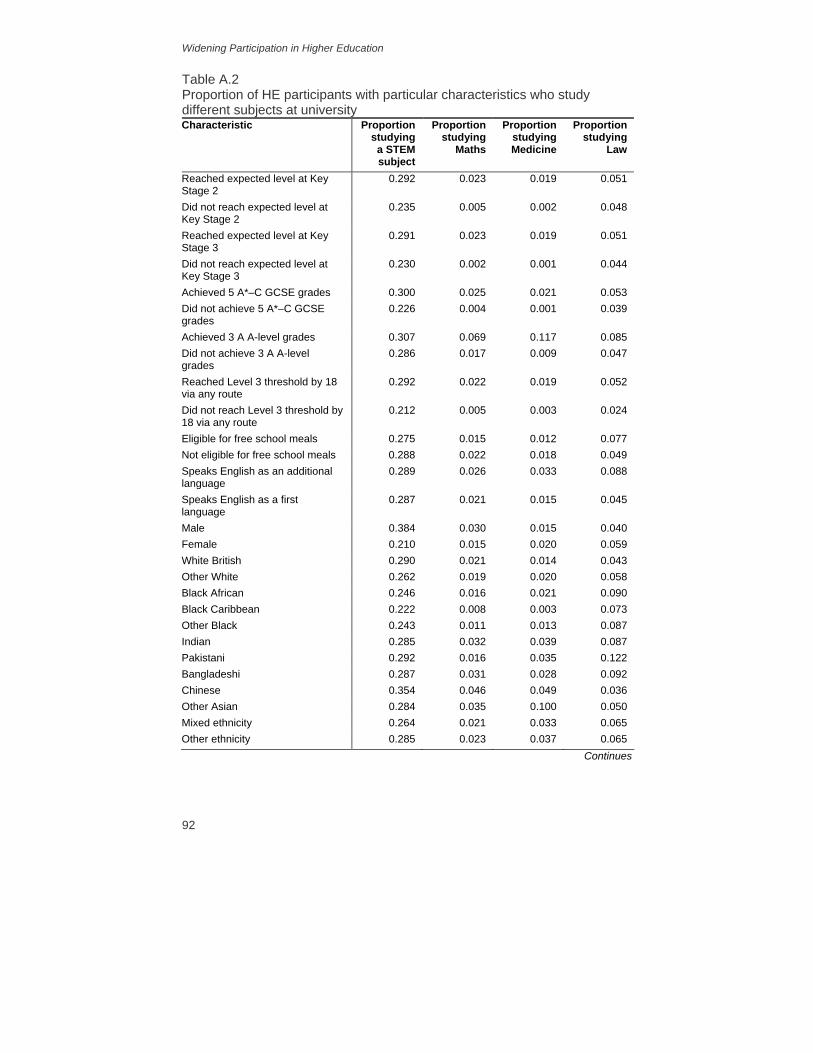
Widening Participation in Higher Education
92
Table A.2 Proportion of HE participants with particular characteristics who study different subjects at university Characteristic Proportion
studyinga STEM subject
Proportion studying
Maths
Proportion studying Medicine
Proportion studying
Law
Reached expected level at Key Stage 2
0.292 0.023 0.019 0.051
Did not reach expected level at Key Stage 2
0.235 0.005 0.002 0.048
Reached expected level at Key Stage 3
0.291 0.023 0.019 0.051
Did not reach expected level at Key Stage 3
0.230 0.002 0.001 0.044
Achieved 5 A*–C GCSE grades 0.300 0.025 0.021 0.053 Did not achieve 5 A*–C GCSE grades
0.226 0.004 0.001 0.039
Achieved 3 A A-level grades 0.307 0.069 0.117 0.085 Did not achieve 3 A A-level grades
0.286 0.017 0.009 0.047
Reached Level 3 threshold by 18 via any route
0.292 0.022 0.019 0.052
Did not reach Level 3 threshold by 18 via any route
0.212 0.005 0.003 0.024
Eligible for free school meals 0.275 0.015 0.012 0.077 Not eligible for free school meals 0.288 0.022 0.018 0.049 Speaks English as an additional language
0.289 0.026 0.033 0.088
Speaks English as a first language
0.287 0.021 0.015 0.045
Male 0.384 0.030 0.015 0.040 Female 0.210 0.015 0.020 0.059 White British 0.290 0.021 0.014 0.043 Other White 0.262 0.019 0.020 0.058 Black African 0.246 0.016 0.021 0.090 Black Caribbean 0.222 0.008 0.003 0.073 Other Black 0.243 0.011 0.013 0.087 Indian 0.285 0.032 0.039 0.087 Pakistani 0.292 0.016 0.035 0.122 Bangladeshi 0.287 0.031 0.028 0.092 Chinese 0.354 0.046 0.049 0.036 Other Asian 0.284 0.035 0.100 0.050 Mixed ethnicity 0.264 0.021 0.033 0.065 Other ethnicity 0.285 0.023 0.037 0.065
Continues

Appendix A
93
Table A.2 continued Characteristic Proportion
studyinga STEM subject
Proportion studying
Maths
Proportion studying Medicine
Proportion studying
Law
Least deprived quintile 0.289 0.023 0.021 0.044 2nd deprivation quintile 0.294 0.022 0.019 0.042 3rd deprivation quintile 0.284 0.021 0.015 0.052 4th deprivation quintile 0.281 0.020 0.014 0.059 Most deprived quintile 0.278 0.018 0.014 0.076 Least educated quintile 0.283 0.016 0.006 0.058 2nd OA education quintile 0.288 0.019 0.010 0.056 3rd OA education quintile 0.290 0.021 0.013 0.051 4th OA education quintile 0.293 0.021 0.018 0.049 Most educated quintile 0.281 0.024 0.025 0.047 Attends a community school 0.292 0.020 0.014 0.051 Attends a foundation school 0.287 0.023 0.022 0.050 Attends a voluntary aided school 0.272 0.023 0.023 0.050 Attends a voluntary controlled school
0.294 0.023 0.022 0.041

94
APPENDIX B Characteristics of HE Participants who
Study Maths or Medicine Table B.1 Personal characteristics of HE participants who study Maths and HE participants who do not Characteristic Study
Maths In HE but
do not study Maths
Difference
Reached expected level at Key Stage 2 0.980 0.908 0.072*** Reached expected level at Key Stage 3 0.993 0.937 0.056*** Achieved 5 A*–C GCSE grades 0.972 0.824 0.148*** Achieved 3 A A-level grades 0.262 0.077 0.185*** Reached Level 3 threshold by 18 via any route 0.988 0.941 0.047*** Eligible for free school meals 0.045 0.065 –0.019*** Speaks English as an additional language 0.155 0.128 0.027*** Male 0.616 0.440 0.177*** White British 0.781 0.802 –0.021*** Other White 0.026 0.029 –0.003*** Black African 0.012 0.016 –0.004*** Black Caribbean 0.004 0.012 –0.008*** Other Black 0.003 0.006 –0.003*** Indian 0.080 0.054 0.027*** Pakistani 0.024 0.032 –0.008*** Bangladeshi 0.015 0.011 0.005*** Chinese 0.017 0.008 0.009*** Other Asian 0.009 0.005 0.004*** Mixed ethnicity 0.011 0.011 0.000 Other ethnicity 0.018 0.017 0.001*** Least deprived quintile 0.341 0.312 0.029*** 2nd deprivation quintile 0.250 0.249 0.002 3rd deprivation quintile 0.193 0.196 –0.003*** 4th deprivation quintile 0.129 0.140 –0.012*** Most deprived quintile 0.087 0.102 –0.016*** Least educated quintile 0.060 0.078 –0.018*** 2nd OA education quintile 0.125 0.143 –0.018*** 3rd OA education quintile 0.194 0.199 –0.006*** 4th OA education quintile 0.256 0.256 0.000 Most educated quintile 0.366 0.324 0.042*** Notes: The numbers presented in each column are the mean values of each characteristic for HE participants who study Maths (column 1) and HE participants who do not study Maths (column 2), and the difference between these means (column 3). For all those characteristics taking values either 0 or 1, the mean values in columns 1 and 2 are interpretable as the proportion of HE participants studying Maths or not studying Maths who take the value 1 for that characteristic. *** indicates significance at the 1% level, ** at the 5% level and * at the 10% level.

Appendix B
95
Table B.2 Characteristics of schools attended by HE participants who study Maths and HE participants who do not Characteristic Study
Maths In HE but do
not study Maths
Difference
Proportion of FSM pupils 0.108 0.118 –0.010*** Proportion of EAL pupils 0.108 0.097 0.010*** Proportion of statemented SEN pupils 0.019 0.021 –0.002*** Proportion of non-statemented SEN pupils 0.149 0.160 –0.011*** School-level proportion of non-White pupils 0.167 0.156 0.011*** School average capped Key Stage 4 points 39.075 37.791 1.285*** Is a community school 0.550 0.577 –0.027*** Is a foundation school 0.205 0.189 0.016*** Is a voluntary aided school 0.191 0.181 0.009*** Is a voluntary controlled school 0.047 0.043 0.003*** Notes: See Notes to Table B.1. *** indicates significance at the 1% level, ** at the 5% level and * at the 10% level.
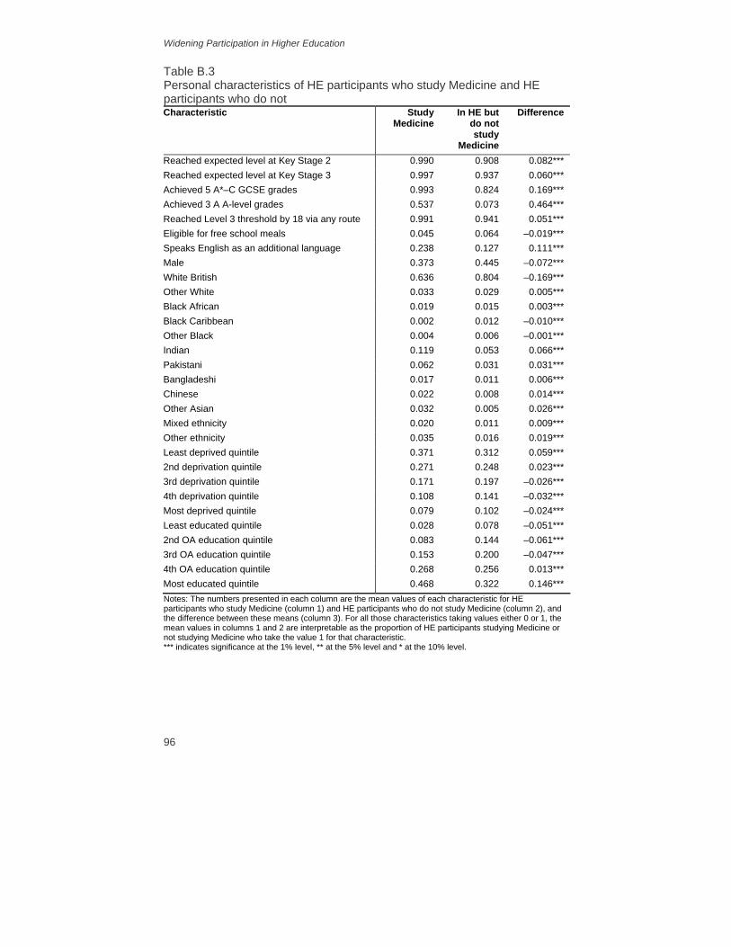
Widening Participation in Higher Education
96
Table B.3 Personal characteristics of HE participants who study Medicine and HE participants who do not Characteristic Study
Medicine In HE but
do not study
Medicine
Difference
Reached expected level at Key Stage 2 0.990 0.908 0.082*** Reached expected level at Key Stage 3 0.997 0.937 0.060*** Achieved 5 A*–C GCSE grades 0.993 0.824 0.169*** Achieved 3 A A-level grades 0.537 0.073 0.464*** Reached Level 3 threshold by 18 via any route 0.991 0.941 0.051*** Eligible for free school meals 0.045 0.064 –0.019*** Speaks English as an additional language 0.238 0.127 0.111*** Male 0.373 0.445 –0.072*** White British 0.636 0.804 –0.169*** Other White 0.033 0.029 0.005*** Black African 0.019 0.015 0.003*** Black Caribbean 0.002 0.012 –0.010*** Other Black 0.004 0.006 –0.001*** Indian 0.119 0.053 0.066*** Pakistani 0.062 0.031 0.031*** Bangladeshi 0.017 0.011 0.006*** Chinese 0.022 0.008 0.014*** Other Asian 0.032 0.005 0.026*** Mixed ethnicity 0.020 0.011 0.009*** Other ethnicity 0.035 0.016 0.019*** Least deprived quintile 0.371 0.312 0.059*** 2nd deprivation quintile 0.271 0.248 0.023*** 3rd deprivation quintile 0.171 0.197 –0.026*** 4th deprivation quintile 0.108 0.141 –0.032*** Most deprived quintile 0.079 0.102 –0.024*** Least educated quintile 0.028 0.078 –0.051*** 2nd OA education quintile 0.083 0.144 –0.061*** 3rd OA education quintile 0.153 0.200 –0.047*** 4th OA education quintile 0.268 0.256 0.013*** Most educated quintile 0.468 0.322 0.146*** Notes: The numbers presented in each column are the mean values of each characteristic for HE participants who study Medicine (column 1) and HE participants who do not study Medicine (column 2), and the difference between these means (column 3). For all those characteristics taking values either 0 or 1, the mean values in columns 1 and 2 are interpretable as the proportion of HE participants studying Medicine or not studying Medicine who take the value 1 for that characteristic. *** indicates significance at the 1% level, ** at the 5% level and * at the 10% level.
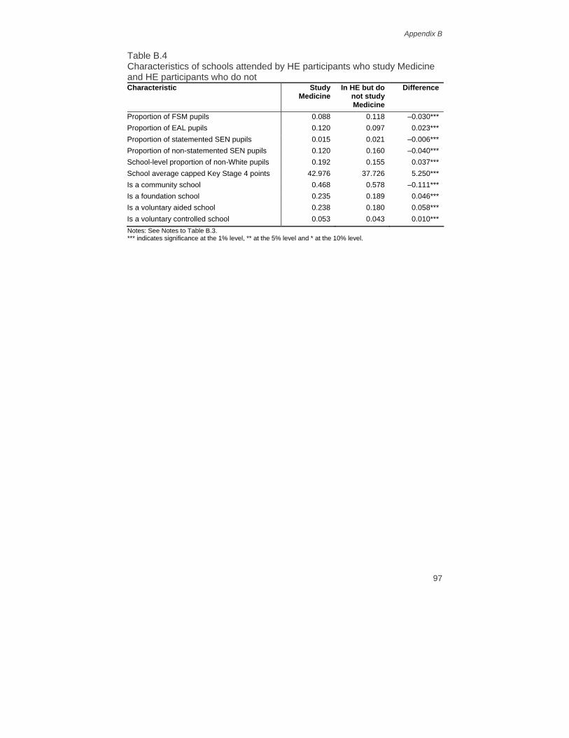
Appendix B
97
Table B.4 Characteristics of schools attended by HE participants who study Medicine and HE participants who do not Characteristic Study
Medicine In HE but do
not study Medicine
Difference
Proportion of FSM pupils 0.088 0.118 –0.030*** Proportion of EAL pupils 0.120 0.097 0.023*** Proportion of statemented SEN pupils 0.015 0.021 –0.006*** Proportion of non-statemented SEN pupils 0.120 0.160 –0.040*** School-level proportion of non-White pupils 0.192 0.155 0.037*** School average capped Key Stage 4 points 42.976 37.726 5.250*** Is a community school 0.468 0.578 –0.111*** Is a foundation school 0.235 0.189 0.046*** Is a voluntary aided school 0.238 0.180 0.058*** Is a voluntary controlled school 0.053 0.043 0.010*** Notes: See Notes to Table B.3. *** indicates significance at the 1% level, ** at the 5% level and * at the 10% level.

98
APPENDIX C Comparison of HE Participants across Years Table C.1 Personal characteristics of HE participants who started in 2004–05 (age 18) and HE participants who started in 2005–06 (age 19) Characteristic Started HE
in 2004–05(age 18)
Started HE in 2005–06
(age 19)
Difference
Reached expected level at Key Stage 2 0.929 0.863 0.065*** Reached expected level at Key Stage 3 0.960 0.887 0.073*** Achieved 5 A*–C GCSE grades 0.869 0.727 0.143*** Achieved 3 A A-level grades 0.096 0.046 0.050*** Reached Level 3 threshold by 18 via any route 0.952 0.918 0.034*** Eligible for free school meals 0.055 0.085 –0.030*** Speaks English as an additional language 0.120 0.148 –0.028*** Male 0.431 0.474 –0.044*** White British 0.813 0.775 0.038*** Other White 0.027 0.033 –0.006*** Black African 0.013 0.021 –0.008*** Black Caribbean 0.010 0.016 –0.005*** Other Black 0.005 0.007 –0.003*** Indian 0.055 0.052 0.003*** Pakistani 0.027 0.042 –0.015*** Bangladeshi 0.010 0.012 –0.002*** Chinese 0.008 0.007 0.002*** Other Asian 0.006 0.005 0.001** Mixed ethnicity 0.011 0.010 0.001*** Other ethnicity 0.015 0.021 –0.006*** Least deprived quintile 0.323 0.287 0.036*** 2nd deprivation quintile 0.253 0.237 0.016*** 3rd deprivation quintile 0.198 0.193 0.004** 4th deprivation quintile 0.135 0.153 –0.018*** Most deprived quintile 0.090 0.129 –0.039*** Least educated quintile 0.075 0.083 –0.007*** 2nd OA education quintile 0.143 0.141 0.003 3rd OA education quintile 0.204 0.189 0.014*** 4th OA education quintile 0.259 0.248 0.011*** Most educated quintile 0.318 0.339 –0.020*** Notes: The numbers presented in each column are the mean values of each characteristic for HE participants who started in 2004–05 at age 18 (column 1) and HE participants who started in 2005–06 at age 19 (column 2), and the difference between these means (column 3). For all those characteristics taking values either 0 or 1, the mean values in columns 1 and 2 are interpretable as the proportion of HE participants starting in 2004–05 or starting in 2005–06 who take the value 1 for that characteristic. *** indicates significance at the 1% level, ** at the 5% level and * at the 10% level.

Appendix C
99
Table C.2 Characteristics of schools attended by HE participants who started in 2004–05 (age 18) and HE participants who started in 2005–06 (age 19) Characteristic Started HE
in 2004–05 (age 18)
Started HE in 2005–06
(age 19)
Difference
Proportion of FSM pupils 0.568 0.596 –0.029*** Proportion of EAL pupils 0.195 0.177 0.018*** Proportion of statemented SEN pupils 0.185 0.174 0.010*** Proportion of non-statemented SEN pupils 0.043 0.044 0.000 School-level proportion of non-White pupils 0.112 0.130 –0.018*** School average capped Key Stage 4 points 0.091 0.112 –0.021*** Is a community school 0.020 0.022 –0.002*** Is a foundation school 0.155 0.170 –0.015*** Is a voluntary aided school 0.149 0.173 –0.025*** Is a voluntary controlled school 38.150 37.039 1.110*** Notes: See Notes to Table C.1. *** indicates significance at the 1% level, ** at the 5% level and * at the 10% level.

100
APPENDIX D Gradients associated with Studying
Maths at University D.1 Males Table D.1 Raw gradients in probability of studying Maths at university, by deprivation quintile, neighbourhood parental education quintile and ethnicity for males Material deprivation Neighbourhood
parental education Ethnicity
Across schools
Within schools
Across schools
Within schools
Across schools
Within schools
4th deprivation quintile
0.002 0.002
3rd deprivation quintile
0.003 0.003
2nd deprivation quintile
0.003 0.003
Least deprived quintile
0.005** 0.005
2nd OA education quintile
–0.001 –0.002
3rd OA education quintile
0.003 0.001
4th OA education quintile
0.004 0.000
Most educated quintile
0.008*** 0.004
Other White –0.002 –0.008* Black African –0.007 –0.009 Black Caribbean –0.020*** –0.022*** Other Black –0.008 –0.004 Indian 0.015*** 0.011** Pakistani –0.011*** –0.010*** Bangladeshi 0.016** 0.016* Chinese 0.045*** 0.043*** Other Asian 0.019* 0.009 Mixed ethnicity 0.002 0.002 Other ethnicity 0.001 –0.004 Constant 0.026*** 0.027*** 0.026*** 0.028*** 0.029*** 0.030*** Observations 67,961 67,961 67,961 67,961 67,961 67,961 R-squared 0.000 0.000 0.000 0.000 0.002 0.001 No. of clusters 2,814 2,814 2,814 Note: The within-schools specification includes school fixed effects (using school attended at age 16). *** indicates significance at the 1% level, ** at the 5% level and * at the 10% level.

Appendix D
101
Table D.2 Gradients in probability of studying Maths at university, controlling for individual-level characteristics (excluding prior attainment) for males Controlling for
deprivation, neighbourhood
parental educationand ethnicity
Plus other individual-level characteristics
4th deprivation quintile 0.000 0.000 3rd deprivation quintile 0.001 0.001 2nd deprivation quintile 0.001 0.001 Least deprived quintile 0.003 0.002
2nd OA education quintile –0.002 –0.002 3rd OA education quintile 0.000 0.000 4th OA education quintile –0.001 –0.001 Most educated quintile 0.003 0.003
Other White –0.008* –0.008* Black African –0.008 –0.008 Black Caribbean –0.021*** –0.021*** Other Black –0.003 –0.003 Indian 0.011** 0.011** Pakistani –0.010** –0.010* Bangladeshi 0.017* 0.017* Chinese 0.044*** 0.043*** Other Asian 0.010 0.009 Mixed ethnicity 0.002 0.002 Other ethnicity –0.004 –0.004
Constant 0.028*** 0.028*** Observations 67,961 67,961 R-squared 0.002 0.002 No. of clusters 2,814 2,814 F-test of additional controls (p-value) 0 0 Notes: All models include school fixed effects (on the basis of school attended at age 16). In addition to deprivation quintile, neighbourhood parental education quintile and ethnicity, column 2 also includes controls for month of birth, whether English is the pupil’s first language and whether they have either statemented (more severe) or non-statemented (less severe) special educational needs (measured at age 16). *** indicates significance at the 1% level, ** at the 5% level and * at the 10% level.

Widening Participation in Higher Education
102
Table D.3 Gradients in probability of studying Maths at university, controlling for individual-level characteristics and prior attainment for males Plus Key
Stage 2 results
Plus Key Stage 3 results
Plus Key Stage 4 results
Plus Key Stage 5 results
Plus Maths
A-level indicator
4th deprivation quintile 0.000 –0.001 –0.001 –0.001 –0.001 3rd deprivation quintile –0.001 –0.002 –0.003 –0.003 –0.002 2nd deprivation quintile –0.002 –0.003 –0.004 –0.004 –0.005 Least deprived quintile 0.000 –0.002 –0.003 –0.004 –0.004
2nd OA education quintile –0.002 –0.003 –0.004 –0.004 –0.004 3rd OA education quintile –0.001 –0.002 –0.003 –0.003 –0.003 4th OA education quintile –0.003 –0.004 –0.005 –0.006* –0.005* Most educated quintile 0.001 –0.001 –0.003 –0.005 –0.004
Other White –0.006 –0.006 –0.006 –0.007 –0.007* Black African –0.002 0.001 0.001 0.002 –0.005 Black Caribbean –0.013*** –0.009* –0.007 –0.006 –0.010** Other Black 0.005 0.007 0.008 0.008 0.004 Indian 0.018*** 0.018*** 0.017*** 0.017*** 0.005 Pakistani –0.001 0.001 0.001 0.001 –0.005 Bangladeshi 0.023** 0.022** 0.021** 0.023** 0.016* Chinese 0.045*** 0.043*** 0.042*** 0.040*** 0.019* Other Asian 0.012 0.010 0.009 0.008 –0.009 Mixed ethnicity 0.002 0.002 0.001 0.001 –0.002 Other ethnicity 0.001 0.001 0.001 0.002 –0.005
Constant –0.003 –0.009* –0.011* –0.015** –0.007 Observations 67,961 67,961 67,961 67,961 67,961 R-squared 0.014 0.019 0.023 0.030 0.086 No. of clusters 2,814 2,814 2,814 2,814 2,814 F-test of additional controls (p-value)
0 0 0 0 0
Note: All models are within-school (i.e. we include school fixed effects on the basis of school attended at age 16). *** indicates significance at the 1% level, ** at the 5% level and * at the 10% level.

Appendix D
103
Table D.4 Gradients in probability of studying Maths at university, controlling for individual-level characteristics and prior attainment in Maths only for males Individual-
level controls
Plus Key Stage 2
Maths
Plus Key Stage 3
Maths
Plus Key Stage 4
Maths
Plus Maths
A-level indicator
4th deprivation quintile 0.000 0.000 0.000 0.000 –0.001 3rd deprivation quintile 0.001 –0.001 –0.002 –0.002 –0.002 2nd deprivation quintile 0.001 –0.002 –0.003 –0.003 –0.005 Least deprived quintile 0.002 –0.001 –0.001 –0.002 –0.004
2nd OA education quintile –0.002 –0.002 –0.002 –0.002 –0.003 3rd OA education quintile 0.000 0.000 –0.001 –0.001 –0.003 4th OA education quintile –0.001 –0.002 –0.003 –0.003 –0.005 Most educated quintile 0.003 0.001 0.001 0.000 –0.003
Other White –0.008* –0.005 –0.006 –0.006 –0.007* Black African –0.008 –0.001 –0.002 –0.002 –0.006 Black Caribbean –0.021*** –0.012** –0.011** –0.010** –0.011** Other Black –0.003 0.006 0.007 0.007 0.004 Indian 0.011** 0.017*** 0.018*** 0.018*** 0.005 Pakistani –0.010* –0.001 0.000 0.000 –0.005 Bangladeshi 0.017* 0.023** 0.023** 0.023** 0.016* Chinese 0.043*** 0.043*** 0.042*** 0.042*** 0.020* Other Asian 0.009 0.012 0.010 0.010 –0.010 Mixed ethnicity 0.002 0.003 0.002 0.002 –0.002 Other ethnicity –0.004 0.000 –0.001 –0.001 –0.007
Constant 0.028*** –0.001 –0.006 –0.007* 0.002 Observations 67,961 67,961 67,961 67,961 67,961 R-squared 0.002 0.019 0.020 0.021 0.086 No. of clusters 2,814 2,814 2,814 2,814 2,814 F-test of additional controls (p-value)
0 0 0 0 0
Note: All models are within-school (i.e. we include school fixed effects on the basis of school attended at age 16). *** indicates significance at the 1% level, ** at the 5% level and * at the 10% level.

Widening Participation in Higher Education
104
D.2 Females Table D.5 Raw gradients in probability of studying Maths at university, by deprivation quintile, neighbourhood parental education quintile and ethnicity for females Material deprivation Neighbourhood
parental education Ethnicity
Across schools
Within schools
Across schools
Within schools
Across schools
Within schools
4th deprivation quintile
0.001 0.000
3rd deprivation quintile
0.002 0.002
2nd deprivation quintile
0.003** 0.003*
Least deprived quintile
0.004*** 0.003*
2nd OA education quintile
0.004** 0.003*
3rd OA education quintile
0.004*** 0.003**
4th OA education quintile
0.005*** 0.003*
Most educated quintile
0.006*** 0.004***
Other White –0.001 –0.004 Black African –0.002 –0.002 Black Caribbean –0.007*** –0.007** Other Black –0.011*** –0.011*** Indian 0.006*** 0.004 Pakistani 0.000 0.002 Bangladeshi 0.004 0.007 Chinese 0.005 0.007 Other Asian 0.010 0.006 Mixed ethnicity –0.001 –0.002 Other ethnicity 0.003 0.003
Constant 0.012*** 0.013*** 0.010*** 0.011*** 0.015*** 0.015*** Observations 85,260 85,260 85,260 85,260 85,260 85,260 R-squared 0.000 0.000 0.000 0.000 0.000 0.000 No. of clusters 2,852 2,852 2,852 Note: The within-schools specification includes school fixed effects (using school attended at age 16). *** indicates significance at the 1% level, ** at the 5% level and * at the 10% level.

Appendix D
105
Table D.6 Gradients in probability of studying Maths at university, controlling for individual-level characteristics (excluding prior attainment) for females Controlling for
deprivation, neighbourhood
parental educationand ethnicity
Plus other individual-level characteristics
4th deprivation quintile 0.000 0.000 3rd deprivation quintile 0.001 0.001 2nd deprivation quintile 0.002 0.002 Least deprived quintile 0.003 0.002
2nd OA education quintile 0.002 0.002 3rd OA education quintile 0.002 0.002 4th OA education quintile 0.002 0.002 Most educated quintile 0.003 0.003
Other White –0.004 –0.004* Black African –0.002 –0.003 Black Caribbean –0.006** –0.006** Other Black –0.011*** –0.011*** Indian 0.005* 0.002 Pakistani 0.003 0.000 Bangladeshi 0.008 0.005 Chinese 0.007 0.005 Other Asian 0.006 0.004 Mixed ethnicity –0.002 –0.002 Other ethnicity 0.003 0.002
Constant 0.011*** 0.010*** Observations 85,260 85,260 R-squared 0.000 0.001 No. of clusters 2,852 2,852 F-test of additional controls (p-value) 0 0 Notes: All models include school fixed effects (on the basis of school attended at age 16). In addition to deprivation quintile, neighbourhood parental education quintile and ethnicity, column 2 also includes controls for month of birth, whether English is the pupil’s first language and whether they have either statemented (more severe) or non-statemented (less severe) special educational needs (measured at age 16). *** indicates significance at the 1% level, ** at the 5% level and * at the 10% level.

Widening Participation in Higher Education
106
Table D.7 Gradients in probability of studying Maths at university, controlling for individual-level characteristics and prior attainment for females Plus Key
Stage 2 results
Plus Key Stage 3 results
Plus Key Stage 4 results
Plus Key Stage 5 results
Plus Maths
A-level indicator
4th deprivation quintile –0.001 –0.001 –0.001 –0.001 –0.002 3rd deprivation quintile 0.000 –0.001 –0.001 –0.001 –0.001 2nd deprivation quintile 0.001 0.000 0.000 0.000 –0.001 Least deprived quintile 0.001 0.000 –0.001 –0.001 –0.001
2nd OA education quintile 0.002 0.001 0.001 0.001 0.001 3rd OA education quintile 0.001 0.001 0.001 0.000 0.000 4th OA education quintile 0.001 0.000 –0.001 –0.001 –0.001 Most educated quintile 0.001 0.000 0.000 –0.001 –0.001
Other White –0.003 –0.003 –0.003 –0.003 –0.004* Black African 0.000 0.001 0.001 0.001 –0.001 Black Caribbean –0.002 0.000 0.000 0.000 –0.002 Other Black –0.007** –0.006* –0.006* –0.006* –0.009** Indian 0.006* 0.005 0.005 0.005 –0.004 Pakistani 0.005 0.006 0.005 0.005 0.002 Bangladeshi 0.009 0.009 0.009 0.009 0.009 Chinese 0.006 0.004 0.003 0.003 –0.018*** Other Asian 0.006 0.005 0.004 0.004 –0.010 Mixed ethnicity –0.002 –0.003 –0.003 –0.003 –0.005 Other ethnicity 0.004 0.004 0.004 0.004 0.000
Constant –0.005** –0.010*** –0.009*** –0.010*** –0.004 Observations 85,260 85,260 85,260 85,260 85,260 R-squared 0.007 0.010 0.011 0.012 0.088 No. of clusters 2,852 2,852 2,852 2,852 2,852 F-test of additional controls (p-value)
0 0 0 0 0
Note: All models are within-school (i.e. we include school fixed effects on the basis of school attended at age 16). *** indicates significance at the 1% level, ** at the 5% level and * at the 10% level.

Appendix D
107
Table D.8 Gradients in probability of studying Maths at university, controlling for individual-level characteristics and prior attainment in Maths only for females Individual-
level controls
Plus Key Stage 2
Maths
Plus Key Stage 3
Maths
Plus Key Stage 4
Maths
Plus Maths
A-level indicator
4th deprivation quintile 0.000 –0.001 –0.001 –0.001 –0.002 3rd deprivation quintile 0.001 0.000 0.000 0.000 –0.001 2nd deprivation quintile 0.002 0.001 0.001 0.001 –0.001 Least deprived quintile 0.002 0.001 0.000 0.000 –0.002
2nd OA education quintile 0.002 0.002 0.002 0.002 0.001 3rd OA education quintile 0.002 0.001 0.001 0.001 0.000 4th OA education quintile 0.002 0.001 0.000 0.000 –0.001 Most educated quintile 0.003 0.001 0.001 0.001 –0.002
Other White –0.004* –0.003 –0.003 –0.003 –0.004* Black African –0.003 0.000 0.001 0.001 –0.001 Black Caribbean –0.006** –0.001 0.000 0.000 –0.001 Other Black –0.011*** –0.008** –0.007** –0.007** –0.008** Indian 0.002 0.005 0.005 0.005 –0.004 Pakistani 0.000 0.004 0.005 0.005 0.002 Bangladeshi 0.005 0.009 0.010 0.010 0.009 Chinese 0.005 0.005 0.004 0.004 –0.018*** Other Asian 0.004 0.005 0.005 0.005 –0.009 Mixed ethnicity –0.002 –0.002 –0.002 –0.002 –0.005 Other ethnicity 0.002 0.003 0.004 0.004 0.000
Constant 0.010*** –0.004* –0.008*** –0.008*** –0.001 Observations 85,260 85,260 85,260 85,260 85,260 R-squared 0.001 0.011 0.012 0.012 0.088 No. of clusters 2,852 2,852 2,852 2,852 2,852 F-test of additional controls (p-value)
0 0 0 0 0
Note: All models are within-school (i.e. we include school fixed effects on the basis of school attended at age 16). *** indicates significance at the 1% level, ** at the 5% level and * at the 10% level.

108
APPENDIX E Gradients associated with Studying
Medicine at University E.1 Males Table E.1 Raw gradients in probability of studying Medicine at university, by deprivation quintile, neighbourhood parental education quintile and ethnicity for males Material deprivation Neighbourhood
parental education Ethnicity
Across schools
Within schools
Across schools
Within schools
Across schools
Within schools
4th deprivation quintile
–0.001 0.001
3rd deprivation quintile
0.000 0.002
2nd deprivation quintile
0.004* 0.005**
Least deprived quintile
0.002 0.001
2nd OA education quintile
0.004** 0.003*
3rd OA education quintile
0.006*** 0.004**
4th OA education quintile
0.010*** 0.007***
Most educated quintile
0.014*** 0.008***
Other White 0.007** 0.012*** Black African 0.008* 0.022*** Black Caribbean –0.008*** 0.004 Other Black –0.008** –0.001 Indian 0.029*** 0.043*** Pakistani 0.023*** 0.037*** Bangladeshi 0.019*** 0.032*** Chinese 0.023*** 0.026*** Other Asian 0.073*** 0.074*** Mixed ethnicity 0.015** 0.013* Other ethnicity 0.020*** 0.028*** Constant 0.013*** 0.013*** 0.006*** 0.009*** 0.011*** 0.009*** Observations 67,961 67,961 67,961 67,961 67,961 67,961 R-squared 0.000 0.000 0.001 0.001 0.007 0.007 No. of clusters 2,814 2,814 2,814 Note: The within-schools specification includes school fixed effects (using school attended at age 16). *** indicates significance at the 1% level, ** at the 5% level and * at the 10% level.

Appendix E
109
Table E.2 Gradients in probability of studying Medicine at university, controlling for individual-level characteristics (excluding prior attainment) for males Controlling for
deprivation, neighbourhood
parental educationand ethnicity
Plus other individual-level characteristics
4th deprivation quintile 0.002 0.002 3rd deprivation quintile 0.004* 0.004* 2nd deprivation quintile 0.008*** 0.008*** Least deprived quintile 0.005* 0.005*
2nd OA education quintile 0.001 0.001 3rd OA education quintile 0.001 0.001 4th OA education quintile 0.004** 0.004** Most educated quintile 0.006** 0.006**
Other White 0.012*** 0.012*** Black African 0.023*** 0.023*** Black Caribbean 0.006* 0.006** Other Black 0.001 0.001 Indian 0.043*** 0.041*** Pakistani 0.039*** 0.038*** Bangladeshi 0.034*** 0.032*** Chinese 0.027*** 0.025*** Other Asian 0.075*** 0.074*** Mixed ethnicity 0.014** 0.014** Other ethnicity 0.029*** 0.028***
Constant 0.001 0.005** Observations 67,961 67,961 R-squared 0.008 0.009 No. of clusters 2,814 2,814 F-test of additional controls (p-value) 0 0 Notes: All models include school fixed effects (on the basis of school attended at age 16). In addition to deprivation quintile, neighbourhood parental education quintile and ethnicity, column 2 also includes controls for month of birth, whether English is the pupil’s first language and whether they have either statemented (more severe) or non-statemented (less severe) special educational needs (measured at age 16). *** indicates significance at the 1% level, ** at the 5% level and * at the 10% level.
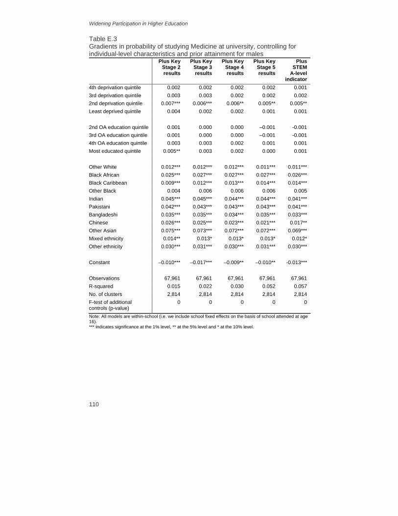
Widening Participation in Higher Education
110
Table E.3 Gradients in probability of studying Medicine at university, controlling for individual-level characteristics and prior attainment for males Plus Key
Stage 2 results
Plus Key Stage 3 results
Plus Key Stage 4 results
Plus Key Stage 5 results
Plus STEM
A-level indicator
4th deprivation quintile 0.002 0.002 0.002 0.002 0.001 3rd deprivation quintile 0.003 0.003 0.002 0.002 0.002 2nd deprivation quintile 0.007*** 0.006*** 0.006** 0.005** 0.005** Least deprived quintile 0.004 0.002 0.002 0.001 0.001
2nd OA education quintile 0.001 0.000 0.000 –0.001 -0.001 3rd OA education quintile 0.001 0.000 0.000 –0.001 -0.001 4th OA education quintile 0.003 0.003 0.002 0.001 0.001 Most educated quintile 0.005** 0.003 0.002 0.000 0.001
Other White 0.012*** 0.012*** 0.012*** 0.011*** 0.011*** Black African 0.025*** 0.027*** 0.027*** 0.027*** 0.026*** Black Caribbean 0.009*** 0.012*** 0.013*** 0.014*** 0.014*** Other Black 0.004 0.006 0.006 0.006 0.005 Indian 0.045*** 0.045*** 0.044*** 0.044*** 0.041*** Pakistani 0.042*** 0.043*** 0.043*** 0.043*** 0.041*** Bangladeshi 0.035*** 0.035*** 0.034*** 0.035*** 0.033*** Chinese 0.026*** 0.025*** 0.023*** 0.021*** 0.017** Other Asian 0.075*** 0.073*** 0.072*** 0.072*** 0.069*** Mixed ethnicity 0.014** 0.013* 0.013* 0.013* 0.012* Other ethnicity 0.030*** 0.031*** 0.030*** 0.031*** 0.030***
Constant –0.010*** –0.017*** –0.009** –0.010** -0.013*** Observations 67,961 67,961 67,961 67,961 67,961 R-squared 0.015 0.022 0.030 0.052 0.057 No. of clusters 2,814 2,814 2,814 2,814 2,814 F-test of additional controls (p-value)
0 0 0 0 0
Note: All models are within-school (i.e. we include school fixed effects on the basis of school attended at age 16). *** indicates significance at the 1% level, ** at the 5% level and * at the 10% level.
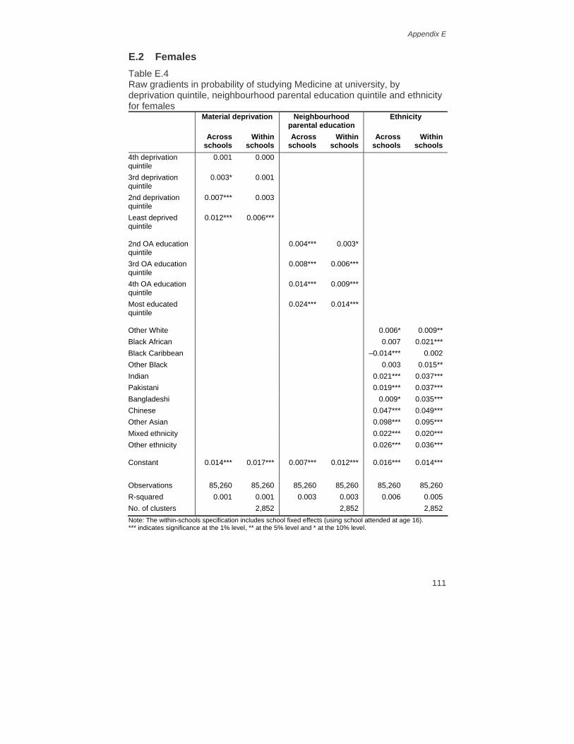
Appendix E
111
E.2 Females Table E.4 Raw gradients in probability of studying Medicine at university, by deprivation quintile, neighbourhood parental education quintile and ethnicity for females Material deprivation Neighbourhood
parental education Ethnicity
Across schools
Within schools
Across schools
Within schools
Across schools
Within schools
4th deprivation quintile
0.001 0.000
3rd deprivation quintile
0.003* 0.001
2nd deprivation quintile
0.007*** 0.003
Least deprived quintile
0.012*** 0.006***
2nd OA education quintile
0.004*** 0.003*
3rd OA education quintile
0.008*** 0.006***
4th OA education quintile
0.014*** 0.009***
Most educated quintile
0.024*** 0.014***
Other White 0.006* 0.009** Black African 0.007 0.021*** Black Caribbean –0.014*** 0.002 Other Black 0.003 0.015** Indian 0.021*** 0.037*** Pakistani 0.019*** 0.037*** Bangladeshi 0.009* 0.035*** Chinese 0.047*** 0.049*** Other Asian 0.098*** 0.095*** Mixed ethnicity 0.022*** 0.020*** Other ethnicity 0.026*** 0.036***
Constant 0.014*** 0.017*** 0.007*** 0.012*** 0.016*** 0.014*** Observations 85,260 85,260 85,260 85,260 85,260 85,260 R-squared 0.001 0.001 0.003 0.003 0.006 0.005 No. of clusters 2,852 2,852 2,852 Note: The within-schools specification includes school fixed effects (using school attended at age 16). *** indicates significance at the 1% level, ** at the 5% level and * at the 10% level.

Widening Participation in Higher Education
112
Table E.5 Gradients in probability of studying Medicine at university, controlling for individual-level characteristics (excluding prior attainment) for females Controlling for
deprivation, neighbourhood
parental educationand ethnicity
Plus other individual-level characteristics
4th deprivation quintile 0.002 0.001 3rd deprivation quintile 0.002 0.002 2nd deprivation quintile 0.004** 0.004* Least deprived quintile 0.006*** 0.006***
2nd OA education quintile 0.001 0.001 3rd OA education quintile 0.004** 0.004** 4th OA education quintile 0.006*** 0.006*** Most educated quintile 0.012*** 0.012***
Other White 0.009** 0.009** Black African 0.024*** 0.023*** Black Caribbean 0.004 0.005* Other Black 0.017** 0.017** Indian 0.038*** 0.036*** Pakistani 0.039*** 0.037*** Bangladeshi 0.037*** 0.035*** Chinese 0.050*** 0.049*** Other Asian 0.096*** 0.094*** Mixed ethnicity 0.021*** 0.021*** Other ethnicity 0.037*** 0.036***
Constant 0.004** 0.003 Observations 85,260 85,260 R-squared 0.008 0.008 No. of clusters 2,852 2,852 F-test of additional controls (p-value) 0 0 Notes: All models include school fixed effects (on the basis of school attended at age 16). In addition to deprivation quintile, neighbourhood parental education quintile and ethnicity, column 2 also includes controls for month of birth, whether English is the pupil’s first language and whether they have either statemented (more severe) or non-statemented (less severe) special educational needs (measured at age 16). *** indicates significance at the 1% level, ** at the 5% level and * at the 10% level.

Appendix E
113
Table E.6 Gradients in probability of studying Medicine at university, controlling for individual-level characteristics and prior attainment for females Plus Key
Stage 2 results
Plus Key Stage 3 results
Plus Key Stage 4 results
Plus Key Stage 5 results
Plus STEM
A-level indicator
4th deprivation quintile 0.001 0.000 0.000 0.000 0 3rd deprivation quintile 0.001 0.000 –0.001 –0.001 -0.001 2nd deprivation quintile 0.003 0.001 0.001 0.000 0 Least deprived quintile 0.004* 0.003 0.002 0.001 0
2nd OA education quintile 0.000 0.000 0.000 –0.001 -0.001 3rd OA education quintile 0.003 0.002 0.001 0.001 0.001 4th OA education quintile 0.005*** 0.004** 0.003* 0.002 0.002 Most educated quintile 0.009*** 0.008*** 0.007*** 0.004** 0.004**
Other White 0.010** 0.010** 0.010** 0.008** 0.007* Black African 0.025*** 0.027*** 0.027*** 0.026*** 0.022*** Black Caribbean 0.010*** 0.012*** 0.012*** 0.012*** 0.011*** Other Black 0.022*** 0.023*** 0.023*** 0.023*** 0.022*** Indian 0.041*** 0.040*** 0.039*** 0.040*** 0.032*** Pakistani 0.043*** 0.045*** 0.044*** 0.045*** 0.038*** Bangladeshi 0.041*** 0.041*** 0.040*** 0.040*** 0.036*** Chinese 0.050*** 0.047*** 0.046*** 0.044*** 0.034*** Other Asian 0.097*** 0.095*** 0.094*** 0.094*** 0.084*** Mixed ethnicity 0.020*** 0.019*** 0.019*** 0.018*** 0.017** Other ethnicity 0.038*** 0.038*** 0.038*** 0.038*** 0.034***
Constant –0.019*** –0.022*** –0.022*** –0.024*** -0.026*** Observations 85,260 85,260 85,260 85,260 85,260 R-squared 0.020 0.029 0.032 0.057 0.076 No. of clusters 2,852 2,852 2,852 2,852 2,852 F-test of additional controls (p-value)
0 0 0 0 0
Note: All models are within-school (i.e. we include school fixed effects on the basis of school attended at age 16). *** indicates significance at the 1% level, ** at the 5% level and * at the 10% level.

114
References
Bekhradnia, B. (2003), Widening Participation and Fair Access: An Overview of the Evidence, Report from the Higher Education Policy Institute.
Belley, P. and Lochner, L. (2007), ‘The changing role of family income and ability in determining educational achievement’, Journal of Human Capital, vol. 1, pp. 37–89.
Blanden, J. and Gregg, P. (2004), ‘Family income and educational attainment: a review of approaches and evidence for Britain’, Oxford Review of Economic Policy, vol. 20, pp. 245–63.
Blanden, J. and Machin, S. (2004), ‘Educational inequality and the expansion of UK higher education’, Scottish Journal of Political Economy, Special Issue on the Economics of Education, vol. 51, pp. 230–49.
Burke, P. (2004), ‘Women accessing education: subjectivity, policy and participation’, Journal of Access Policy and Practice, vol. 1, pp. 100–18.
Callender, C. (2003), ‘Student financial support in higher education: access and exclusion’, in M. Tight (ed.), Access and Exclusion: International Perspectives on Higher Education Research, London: Elsevier Science.
Card, D. and Krueger, A. (1992), ‘Does school quality matter? Returns to education and the characteristics of public schools in the United States’, Journal of Political Economy, vol. 100, pp. 1–40.
Carneiro, P. and Heckman, J. (2002), ‘The evidence on credit constraints in post-secondary schooling’, Economic Journal, vol. 112, pp. 705–34.
Carneiro, P. and Heckman, J. (2003), ‘Human capital policy’, in J. Heckman, A. Krueger and B. Friedman (eds), Inequality in America: What Role for Human Capital Policies?, Cambridge, MA: MIT Press.
Chevalier, A. and Conlon, G. (2003), ‘Does it pay to attend a prestigious university?’, Centre for the Economics of Education (CEE), Discussion Paper no. 33.
Chowdry, H., Crawford, C., Dearden, L., Goodman, A. and Vignoles, A. (2008), ‘Understanding the determinants of participation in higher education and the quality of institute attended: analysis using administrative data’, Institute for Fiscal Studies, mimeo.
CMPO (2006), Family Background and Child Development up to Age 7 in the Avon Longitudinal Survey of Parents and Children (ALSPAC), DfES Research Report no. RR808A.
Connor, H., Burton, R., Pearson, R., Pollard, E. and Regan, J. (1999), Making the Right Choice: How Students Choose University and Colleges, London: Institute for Employment Studies (IES).
Connor, H. and Dewson, S. with C. Tyers, J. Eccles, J. Regan and J. Aston (2001), Social Class and Higher Education: Issues Affecting Decisions on Participation by Lower Social Class Groups, DfES Research Report no. 267.
Connor, H., Tyers, C., Modood, R. and Hillage, J. (2004), Why the Difference? A Closer Look at Higher Education Minority Ethnic Students and Graduates, DfES Research Report no. 552.

References
115
Cunha, F. and Heckman, J. (2007), ‘The technology of skill formation’, American Economic Review, vol. 92, pp. 31–47.
Cunha, F., Heckman, J., Lochner, L. and Masterov, D. (2006), ‘Interpreting the evidence on life cycle skill formation’, in E. Hanushek and F. Welch (eds), Handbook of the Economics of Education, Amsterdam: North-Holland.
Dearing, R. (1997), Higher Education in the Learning Society, Report of the National Committee of Inquiry into Higher Education, Norwich: HMSO.
Demack, S., Drew, D. and Grimsley, M. (2000), ‘Minding the gap: ethnic, gender and social class differences in attainment at 16, 1988–95’, Race, Ethnicity and Education, vol. 3, pp. 112–41.
Department for Education and Skills (2003), Widening Participation in Higher Education, London: DfES (http://www.dfes.gov.uk/hegateway/uploads/EWParticipation.pdf).
Department for Education and Skills (2006), Widening Participation in Higher Education, London: DfES (http://www.dcsf.gov.uk/hegateway/uploads/6820-DfES-WideningParticipation2.pdf).
Feinstein, L. (2003), ‘Inequality in the early cognitive development of British children in the 1970 cohort’, Economica, vol. 70, pp. 73–98.
Forsyth, A. and Furlong, A. (2003), ‘Access to higher education and disadvantaged young people’, British Educational Research Journal, vol. 29, pp. 205–25.
Galindo-Rueda, F., Marcenaro-Gutierrez, O. and Vignoles, A. (2004), ‘The widening socio-economic gap in UK higher education’, National Institute Economic Review, no. 190, pp. 70–82.
Gayle, V., Berridge, D. and Davies, R. (2002), ‘Young people’s entry into higher education: quantifying influential factors’, Oxford Review of Education, vol. 28, pp. 5–20.
Glennerster, H. (2001), ‘United Kingdom education 1997–2001’, Centre for the Analysis of Social Exclusion (CASE), Working Paper no. 50.
Gorard, S. (2000), Education and Social Justice: The Changing Composition of Schools and Its Implications, Cardiff: University of Wales Press.
Gorard, S., Smith, E., May, H., Thomas, L., Adnett, N. and Slack, K. (2006), Review of Widening Participation Research: Addressing the Barriers to Widening Participation in Higher Education, Report to HEFCE by the University of York, Higher Education Academy and Institute for Access Studies, Bristol: HEFCE.
Haggis, T. and Pouget, M. (2002), ‘Trying to be motivated: perspectives on learning from younger students accessing higher education’, Teaching in Higher Education, vol. 7, pp. 323–36.
Haveman, R. and Wolfe, B. (1995), ‘The determinants of children’s attainments: a review of methods and findings’, Journal of Economic Literature, vol. 33, pp. 1829–78.
Heenan, D. (2002), ‘Women, access and progression: an examination of women’s reasons for not continuing in higher education following the completion of the Certificate in Women’s Studies’, Studies in Continuing Education, vol. 24, pp. 40–55.
HEFCE (2005), Young Participation in Higher Education, Bristol: HEFCE (http://www.hefce.ac.uk/pubs/hefce/2005/05_03/05_03.pdf).

Widening Participation in Higher Education
116
Iftikhar, H., McNally, S. and Telhaj, S. (2008), ‘University quality and graduate wages in the UK’, Centre for Economics of Education, mimeo; output from ESRC-TLRP project ‘Widening Participation in Higher Education: A Quantitative Analysis’.
Machin, S. and Vignoles, A. (2004), ‘Educational inequality: the widening socio-economic gap’, Fiscal Studies, vol. 25, pp. 107–28.
Meghir, C. and Palme, M. (2005), ‘Educational reform, ability, and family background’, American Economic Review, vol. 95, pp. 414–24.
Osborne, M., Marks, A. and Turner, E. (2004), ‘Becoming a mature student: how adult applicants weigh the advantages and disadvantages of higher education’, Higher Education: The International Journal of Higher Education and Educational Planning, vol. 48, pp. 291–315.
Pennell, H. and West, A. (2005), ‘The impact of increased fees on participation in higher education in England’, Higher Education Quarterly, vol. 59, pp. 127–37.
Powdthavee, N. and Vignoles, A. (2008), ‘Mature students: a success story?’, Institute of Education, Working Paper.
Quinn, J. (2004), ‘Understanding working-class “drop-out” from higher education through a socio-cultural lens: cultural narratives and local contexts’, International Studies in Sociology of Education, vol. 14, pp. 57–74.
Raffe, D., Croxford, L., Iannelli, C., Shapira, M. and Howieson, C. (2006), Social-Class Inequalities in Education in England and Scotland, Special CES Briefing no. 40, Edinburgh: Centre for Educational Sociology.
Reay, D. (2003), ‘A risky business? Mature working-class women students and access to higher education’, Gender and Education, vol. 15, pp. 301–17.
Rutter, M., Moffitt, E. and Caspi, A. (2006), ‘Gene–environment interplay and psychopathology: multiple varieties but real effects’, Journal of Child Psychology and Psychiatry, vol. 47, pp. 226–61.
Sammons, P. (1995), ‘Gender, ethnic and socio-economic differences in attainment and progress: a longitudinal analysis of student achievement over 9 years’, British Educational Research Journal, vol. 21, pp. 465–85.
Strand, S. (1999), ‘Ethnic group, sex and economic disadvantage: associations with pupil’s educational progress from Baseline to the end of Key Stage 1’, British Educational Research Journal, vol. 25, pp. 179–202.
Sutton Trust (2008), University Admissions by Individual Schools, London (http://www.suttontrust.com/reports/UniversityAdmissions.pdf).
Tomlinson, S. (2001), ‘Some success, could do better: education and race 1976–2000’, in R. Phillips and J. Furlong (eds), Education, Reform and the State: Twenty-Five Years of Politics, Policy and Practice, London: Routledge.
Universities UK (2007), Variable Tuition Fees in England: Assessing their Impact on Students and Higher Education Institutions, London: UUK.
Walker, I. and Zhu, Y. (2005), ‘The college wage premium, over education and the expansion of higher education in the UK’, University of Warwick, mimeo.
Wilson, D., Burgess, S. and Briggs, A. (2005), ‘The dynamics of school attainment of England’s ethnic minorities’, Centre for Market and Public Organisation (CMPO), Working Paper no. 05/130.