Copyright © 2011 by Daniel Bergstresser and Randolph Cohen

Working papers are in draft form. This working paper is distributed for purposes of comment and discussion only. It may not be reproduced without permission of the copyright holder. Copies of working papers are available from the author.

Why fears about municipal credit are overblown Daniel Bergstresser Randolph Cohen

Working Paper

11-129

Why fears about municipal credit are overblown

Daniel Bergstresser* Randolph Cohen**

(First version April 2011. Current draft June 2011. Comments welcome)

Abstract

Highly publicized predictions of 50-100 municipal defaults have caused anxiety among municipal bond investors. While there is some chance that negative investor sentiment will lead to further spread widening, the probability of the kind of widespread default that would be required to justify current municipal bond yields is low. In this paper we document the reasons why the fears of widespread municipal default during the current recession are overblown. Keywords: Municipal bonds.

We are grateful for support from Harvard Business School. Although both authors’ primary affiliations are with academic institutions, both authors have at times been paid for consulting engagements in the investment management industry. Details are available upon request. * Corresponding author. Harvard Business School. Tel.: 617-495-6169. E-mail: dbergstresser@hbs.edu ** Massachusetts Institute of Technology.

1

Contents

1. Summary 2. Why do states and localities borrow in the United States? 3. Do state balanced budget restrictions really matter? 4. How indebted are states and localities today? 5. What is the loss experience on municipal debt? 6. What about investor flows? 7. What about reduced Recovery Act funding for states and localities? 8. What about the declining credit quality of financial guarantors? 9. What about proposals that would allow states to file for bankruptcy protection? 10. Municipal crisis case studies

a. Vallejo, CA b. Boise County, ID c. Jefferson County, AL d. Harrisburg, PA

11. References 12. Exhibits

2

1. Summary

Highly publicized predictions of 50-100 municipal defaults have caused anxiety among municipal bond

investors.1 These recent predictions must be placed into appropriate context, looking both forward and to

history:

In 2009 municipal issuers defaulted on 178 individual bond issues. The aggregate face value of

the defaulted issues was $3.5 Billion. In 2010 issuers defaulted on seventy-five municipal bond

issues, with an aggregate face value of $1.7 Billion.

The municipal credit market is a $2.5 Trillion market.

Thus the prediction of hundreds of municipal defaults has already been realized. Losses have

amounted to a tiny fraction of market value.2

As of December 31, 2010 the MCDX 5-year index spread was 218 basis points. With seventy

percent recovery for investors in default, this spread is consistent with 3.63 defaults per year out

of the index’s fifty names, or a seven percent annual default rate.3

Market spreads as of December 31 were already consistent with approximately thirty percent of

municipal issuers going into default over the next five years. In that sense, the worst of the

doomsday scenarios had already been incorporated into market yields.

This doomsday scenario is very unlikely. States, counties, and cities face long-term budget stress,

related in large part to employee retirement benefits. These problems, though large, are long-

term problems and are unlikely to create across-the-board short-term liquidity crises that could

lead to widespread municipal default.

                                                            1 A recent quote from Meredith Whitney, interviewed on CBS’ 60 Minutes: ‘There’s not a doubt in my mind that you will see a spate of municipal bond defaults…You could see 50 sizeable defaults. 50 to 100 sizeable defaults. More. This will amount to hundreds of billions of dollars worth of defaults.’ See CBS News, December 2010. Even more recently, Whitney has moderated her predictions. In a March 21, 2011 interview with Maria Bartiromo, she noted that ‘Every day things get better because politicians are addressing the fiscal challenges more directly. Since November you’ve had more governors take strong austerity measures.’ See USA Today, March 21, 2011. 2 A recent quote from Jeffrey Gundlach of DoubleLine Capital, interviewed in Barrons: ‘I don’t know whether the market would suffer $10 Billion or $30 Billion in defaults, but the actual amount doesn’t matter.’ $30 Billion in defaults, at historically prevailing recovery rates, would amount to a loss of 40 basis points in the $2.5 Trillion municipal credit market. 3 Expectation on a risk-neutral basis. Please see section on investor flows.

3

In sum, fears of widespread municipal default are overblown. Although spreads have

tightened somewhat since December, doomsday scenarios have already been incorporated into

market prices. While there is a good chance that negative investor sentiment will lead to further

spread widening, the probability of the kind of widespread default that would be required to

justify current municipal bond yields is low.

2. Background: why do states and localities borrow in the United States?

Under the 10th Amendment to the United States Constitution, the fifty individual states retain power over

facets of government that are not explicitly constrained or turned over to the Federal government. This

means that in the United States areas like elementary, secondary, and higher education, law enforcement

and corrections, and public assistance are generally left to state and local control. Each state has its own

constitution, and these individual constitutions often very detailed and specific (unlike the United States

Constitution) about state and local spending, borrowing, and taxing. Within the states, the authority of

cities and counties is established by state legislatures. Their abilities to tax, spend, and borrow vary from

state to state.

Municipal authorities borrow for two primary reasons. First, they borrow to fund infrastructure projects.

Borrowing to fund an infrastructure project such as a school, road, or hospital aligns the timing of

payment and benefits: if a road will have a useful life of 30 years, borrowing to pay for the road over 30

years means that the same generation will both pay for and use the road. Borrowing is also used when

infrastructure projects are immediately necessary in order to comply with federal or other guidelines.

For example, a municipal wastewater treatment facility may require immediate upgrades to comply with

federal standards. Municipal borrowing to fund a project like this would be the only way to avoid sudden

cuts in other services or increases in taxes.

States and localities also occasionally borrow on a short-term basis because the seasonal timing of

municipal receipts does not match the timing of expenditures. In these situations, states and localities

issue short-term instruments (often called Revenue Anticipation Notes or Grant Anticipation Notes) to

cover the time period between expenditures and receipts.

4

There are some important differences between states budget processes and the budget processes that

prevail among sovereigns.4 Forty-four of the fifty states have constitutional or statutory requirements

mandating that the governor submit a balanced budget to the legislature. Thirty-seven states have a

requirement that the final budget be balanced. In principle, only seven states5 allow a deficit to be carried

from one year to the next. As the next section discusses, these restrictions are not always as binding as

they appear at first blush. But they do appear to have an impact on state responses to economic

downturns. A GAO survey (GAO, 1993) estimated that during the 1988-1992 recession forty-nine

percent of the deficit reduction came through spending cuts, and another thirty-two percent was achieved

through revenue increases. The remainder was closed with borrowing, drawing down ‘rainy-day’ funds,

and other (often dubious) accounting adjustments.6

To the extent that they are followed, these limitations on borrowing and carrying forward deficits expose

states to cyclical volatility. State revenues tend to be pro-cyclical, rising with economic activity and

falling in recessions. Expenditures, in particular for public assistance, are often highest in economic

troughs. With borrowing to cover operating deficits generally limited by constitution or statute, states are

often forced to cut services or raise taxes at the bottom of the economic cycle.7

The cuts to state and local services during the recent economic recession have been rapid and steep.

According to the National Association of State Budget Officers (NASBO) 2010 Fiscal Survey of States,

state general fund expenditures fell from $660.9 Billion to $612.6 Billion between fiscal 2009 and fiscal

2010.8 One particular indicator of the depth of the current recession is the extent of state budget cuts that

have been made after annual state budgets have been passed. These post-budget spending cuts reflect

downside ‘surprises’ in revenues, surprises that need to be accommodated using within-year spending

cuts. Figure 1 shows the pattern of within-period budget cuts back to 1990.9 The post-budget cuts during

                                                            4 See NASBO, 2008. 5 California, Indiana, Maine, Michigan, Vermont, Washington, and Wisconsin. 6 Of this remaining 19 percent, 32 (or 6 percent of the total) percent came from drawing down rainy-day funds, 22 percent came from inter-fund transfers, 17 percent came from short-term borrowing, and 13 percent came from deferring payments. Rainy-day funds are state reserves of liquid assets used to cover expenditures during fiscal emergencies. Aggregate rainy day fund balances at the end of 2010 were estimated by the National Association of State Budget Officers to total $27.6 billion. 7 For example, the state legislature in Illinois recently voted to raise personal income taxes by 66 percent in order to balance the 2011 budget, and the governor of California has proposed to reduce higher education funding by $1 billion. NASBO, 2010 describes state-by-state approaches to balancing budgets during the recent economic recession. 8 Under government accounting practices, the General Fund accounts for all financial resources except for those that are specifically required, either by law or by accounting standards, to be accounted for in a different fund. Many states and localities have statutory or constitutional requirements to establish separate funds used exclusively for particular projects. For example, Article IX of the Michigan Constitution creates the State School Aid Fund, which is used exclusively for lower and higher education and for the school employee retirement systems. 9 Reproduced from NASBO, 2010.

5

the current recession have exceeded the cuts of the past two recessions, indicating the severity of the

current recession relative to the milder earlier recessions.

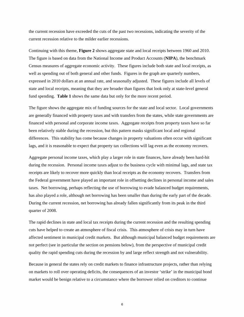
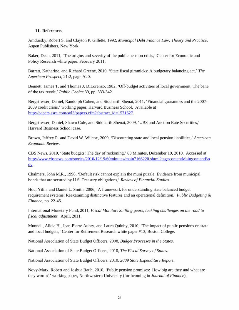
Continuing with this theme, Figure 2 shows aggregate state and local receipts between 1960 and 2010.

The figure is based on data from the National Income and Product Accounts (NIPA), the benchmark

Census measures of aggregate economic activity. These figures include both state and local receipts, as

well as spending out of both general and other funds. Figures in the graph are quarterly numbers,

expressed in 2010 dollars at an annual rate, and seasonally adjusted. These figures include all levels of

state and local receipts, meaning that they are broader than figures that look only at state-level general

fund spending. Table 1 shows the same data but only for the more recent period.

The figure shows the aggregate mix of funding sources for the state and local sector. Local governments

are generally financed with property taxes and with transfers from the states, while state governments are

financed with personal and corporate income taxes. Aggregate receipts from property taxes have so far

been relatively stable during the recession, but this pattern masks significant local and regional

differences. This stability has come because changes in property valuations often occur with significant

lags, and it is reasonable to expect that property tax collections will lag even as the economy recovers.

Aggregate personal income taxes, which play a larger role in state finances, have already been hard-hit

during the recession. Personal income taxes adjust to the business cycle with minimal lags, and state tax

receipts are likely to recover more quickly than local receipts as the economy recovers. Transfers from

the Federal government have played an important role in offsetting declines in personal income and sales

taxes. Net borrowing, perhaps reflecting the use of borrowing to evade balanced budget requirements,

has also played a role, although net borrowing has been smaller than during the early part of the decade.

During the current recession, net borrowing has already fallen significantly from its peak in the third

quarter of 2008.

The rapid declines in state and local tax receipts during the current recession and the resulting spending

cuts have helped to create an atmosphere of fiscal crisis. This atmosphere of crisis may in turn have

affected sentiment in municipal credit markets. But although municipal balanced budget requirements are

not perfect (see in particular the section on pensions below), from the perspective of municipal credit

quality the rapid spending cuts during the recession by and large reflect strength and not vulnerability.

Because in general the states rely on credit markets to finance infrastructure projects, rather than relying

on markets to roll over operating deficits, the consequences of an investor ‘strike’ in the municipal bond

market would be benign relative to a circumstance where the borrower relied on creditors to continue

6

covering operating deficits. It is true that if bond buyers stopped purchasing new bonds today, new

infrastructure projects would become difficult or impossible to finance. The average age of roads, school,

hospitals, and jails would rise, and their quality would deteriorate. But the bonds that had financed those

projects are very likely to be repaid.

3. Do state balanced budget restrictions really matter?

The previous section noted the near-universal existence of state balanced budget requirements. The true

nature of these balanced budget requirements can often be more flexible than they appear at first. A

variety of legal and accounting maneuvers are often available for states to avoid cuts to services in the

face of significant budget problems. A recent paper by Hou and Smith (2006) documents the flexibility

behind state balanced budget requirements. In addition to demonstrating the cross-state differences in the

stringency of these requirements, they show how well-informed observers can even come to different

conclusions about the stringency of the balanced budget requirements for a particular state.10

Surprisingly, many states allow a budget to be considered ‘balanced’ if they can borrow to cover the

deficit. In the last year both Connecticut and New Hampshire have borrowed in order to ‘balance

budgets.’ New Hampshire issued $51 million worth of Debt Service bonds to pay for current debt

payments. Cathy Provencher, New Hampshire Treasury Secretary, noted that this method of balancing

the budget was unprecedented for the state of New Hampshire, and the practice appears to remain

unusual.

There is also significant heterogeneity across states in the extent to which balanced budget requirements

are legally enforced. At one extreme, the Oklahoma Constitution mandates that appropriations from a

fund be reduced pro-rata if revenues fall below forecast. This turns out to be a rather binding

implementation. Alternatively, Virginia has a constitutional requirement that the governor maintain

spending below revenues, but does not appear to have any legal mechanism for enforcing this

requirement. The Michigan Constitution allows ‘unavoidable’ deficits to be carried over to the next fiscal

year, and does not define ‘unavoidable.’

                                                            10 See also Poterba (1995) for a review of the literature on the impact of balanced budget rules. Bennett and DiLorenzo (1982) point to the introduction of Tax and Expenditure Limitations, which occurred during the 1970s and 1980s, as a driving force between the adoption of fiscally evasive tools. They note that state and local governments responded to the TELs by placing billions of dollars of expenditure off-budget, into what they describe as ‘Off-Budget Enterprises’ or OBEs. These OBES are generally financed by revenue bonds, which are often not subject to the same restrictions as general obligation debt.

7

Poterba (1995) points out that exact nature of a balanced budget requirement can depend on the stage of

the budget process at which balanced is required. In New Hampshire, the governor is required by statute

to submit a balanced budget, but there is no requirement that the legislature pass or that the governor sign

a budget that is balanced. Table 2, based on data from the NASBO 2008 Budget Practices in the States,

shows cross-state variation in the actual nature of balanced budget requirements. Poterba (1995)

concludes that the stringency of balanced budget requirements does have an impact on state fiscal

responses to unexpected deficits. States with more stringent rules adjust to deficit overruns with much

larger expenditure cuts than other states. The GAO estimates cited above, which reflect averages across

all of the states, thus mask significant heterogeneity across states in the response of expenditures to

budget shocks.

Focusing on the specific tools for ‘balancing budgets,’ other approaches include the delay of tax refunds,

delaying payments to vendors, and deferring funding of pension plans. The current recession has also

seen some high-profile asset sales by states. As Barrett and Greene (2010) note, Arizona recently sold off

$737 million worth of state assets, which generated money to close a current budget gap. The state will

now have to lease back space in offices it once owned. In that sense, the state’s sale-leaseback represents

the economic equivalent of a debt issue. Barrett and Greene note similar long-term costs to delaying

payments to vendors: over time, vendors build in higher margins to compensate for these payment delays.

Issuing short-term debt is another gimmick identified by the GAO as a tool for balancing budgets during

fiscal crises. Thus one sign of fiscal trouble for state and local borrowers is increasing reliance on the

issuance of short-term debt. Figure 1 suggests that net debt issuance during the recent recession had

already peaked, and was in any case smaller than the net debt issuance during and following the 2001

recession. These aggregate figures mask cross-state variation, however, and Table 3 shows, state-by-

state, total issuance of municipal debt and issuance of short-term debt (defined here as debt with a

maturity of less than 24 months) since the beginning of 2010. The table includes debt issued at both state

and local level, and the final column scales the total short-term issuance by expressing it as a share of

state GDP. Based on this measure, state and local borrowers in California, New Jersey, Massachusetts,

Michigan, and Wisconsin have each issued short-term debt amounting to more than 1 percent of state

GDP in the period since 2010. In no state has short-term borrowing since 2010 exceeded 1.5 percent of

GDP. The size of the gaps identified in Table 3 appears consistent with significant budget stress, but does

not appear large enough to cause widespread liquidity problems like those that are now occurring in parts

of Europe.

8

To be more specific on the comparison to sovereign borrowers, Table 4 shows gross financing needs for a

selection of developed economies for the period between 2010 and 2012. The table is reproduced from a

recent International Monetary Fund report (IMF, 2011). Average budget deficits in this sample of

countries are 8.7 percent of GDP in 2010 and 8.1 percent of GDP in 2011. On top of those deficits,

maturing debt as a share of GDP is 17.2 percent in 2010 and 18.9 percent in 2011. Total gross financing

needs for these sovereign borrowers amount annually to a quarter of GDP for the next several years.

State and local budgets are under stress, and some states are relying on short-term debt issuance and other

types of fiscal gimmicks. But it is fair to say that the picture is worse for the sovereign borrowers

highlighted in the IMF report.

The largest channel for municipal fiscal evasion is pensions, an issue that receives specific coverage in a

section below. On the whole, the flexibility of the balanced budget rules makes it more accurate to say

that states have very strong and long-standing traditions of running balanced budgets, and that these

traditions are generally backed up by some form of legal protection. Over time there is a risk that fiscal

evasion and gimmicks will become increasingly accepted; the unprecedented actions of the current

recession may be viewed as time-honored traditions during the next one. In addition, states and localities

that balance budgets by selling off assets will eventually find that all of their monetizable assets have

been liquidated. Cities that use asset sales and other budget gimmicks to postpone fiscal adjustments will

eventually face very abrupt tax increases or service cuts. This is the situation now in Harrisburg, PA,

which is covered in a case study in the final section below.

But balanced budget requirements, though not perfect, do appear to have an effect. Most of the

adjustments in cyclical downturns come through tax increases and service cuts, and the states with more

stringent balanced budget requirements adjust using deeper expenditure cuts. It is very likely that a

combination of economic recovery and other factors will allow states and localities to weather the current

recession. The current recession will not be the last, however, and the states and localities that continue

to rely on evasive budget practices will be more vulnerable during the next cyclical downturn.

4. How indebted are states and municipalities today?

The section above describes a variety of budget gimmicks that can be used to balance budget, but by far

the biggest hole in state and local balanced budget requirements comes from their sponsorship of defined

benefit pension plans. In fact, the measurement of net state and local borrowing depends crucially on the

accurately measuring pension liabilities.

9

Defined benefit pension programs can be viewed as functionally equivalent to debt. For example, if a

state employee accepts a generous pension plan in exchange for low wages today, then the state has

effectively borrowed from the employee rather than borrowing from capital markets. The rapid increase

in the amount by which state and local pensions are underfunded reflects the use of pension programs to

relax municipal budget constraints.

The accounting rules applied to states and cities do not accurately reflect the true value of their pension

liabilities. This pension accounting problem goes hand-in-hand with the generosity of many municipal

pension arrangements. The programs are particularly generous and their costs have not been reflected

accurately.

Pension promises are long-duration promises. Their current value is sensitive to the discount rate

assumption used to value them. Municipalities, with the blessing of the Government Accounting

Standard Board, continue to use inappropriately high discount rates for valuing these long-term pension

liabilities. The inappropriately high discount rates deliver inappropriately low measures of true municipal

pension liabilities.

A recent paper by Robert Novy-Marx and Joshua Rauh shows the impact of this discount rate assumption

on pension liability valuation. Table 5, reproduced from their paper, shows state-by-state levels of state

municipal debt and of a more comprehensive net debt measure that includes the net pension liability,

measured using the Treasury rate as the discount rate for these liabilities. The use of the Treasury rate to

discount these liabilities increases their magnitude and has a significant impact on measured state

indebtedness. In aggregate, official state debt as a share of GDP was seven percent in 2009. But using

the broader measure of net debt, Novy-Marx and Rauh show that net liabilities amounted to twenty-five

percent of GDP.

The details of the Novy-Marx and Rauh calculations have been the topic of substantial debate, but the

broad thrust of their argument is certainly true: pensions are seriously underfunded.11 Figure 3 uses data

from the Federal Reserve’s Flow of Funds reports and the Census Bureau’s National Income and Product

Accounts to show the evolution of state borrowing over time. The figure shows state and local

borrowing, interest payments, and a broader measure of debt (including gross pension liabilities) as a

share of GDP. While the state borrowing measure in Table 4 does not include city and county bonds,

Figure 1 does. The gross pension liability reflects state reporting of their own liabilities, and is almost

                                                            11 See, among others, Baker 2011, and Brown and Wilcox 2009. From Brown and Wilcox: ‘Nearly all state and local pension defined benefit plans compute the present value of their future liabilities using the expected return on the assets held in the pension trust. This practice contrasts sharply with finance theory, which is unambiguous that the appropriate discount rate is one that reflects the riskiness of the liabilities, not the assets.’

10

surely an underestimate of their true value. But the figure does not include the substantial assets that

partially offset those pension liabilities.

Both explicit debt and interest payments as a share of GDP peaked in the 1980s and early 1990s. Interest

payments have fallen from 1 percent of GDP to under .80 percent of GDP since the 1980s. While debt

amounts have risen over the past 10 years, they are still below the peak reached in the early 1990s.

Including the gross value of pension liabilities suggests that total debt relative to GDP (not including the

value of pension assets) has varied between 30 percent and 40 percent since the early 1990s.

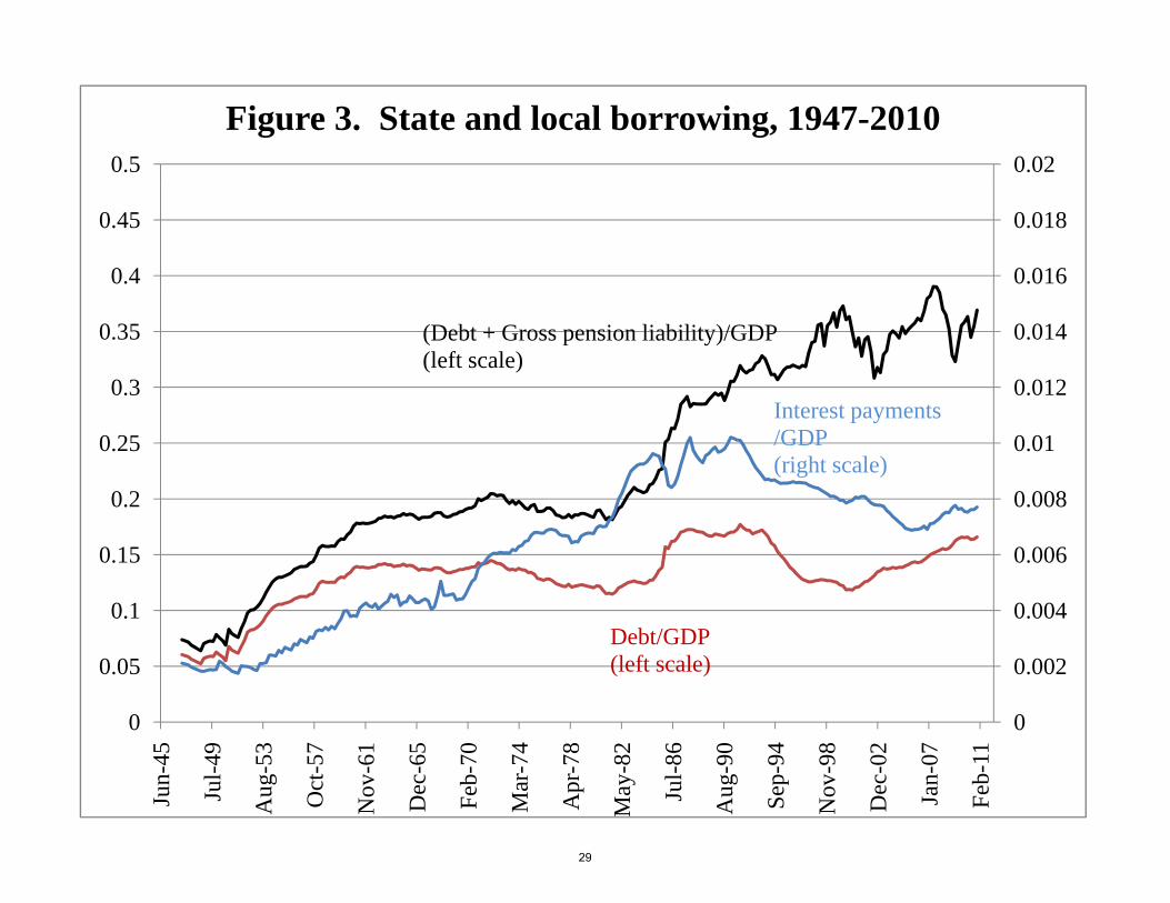
But neither the explicit debt nor the pension debt seem likely to cause widespread liquidity crises during

the current recession. Both forms of debt are very long-term debt. Figure 4 shows the maturity profile of

explicit municipal debt as of early 2011. The maturity profile is very smooth over the next 30 years, with

no more than 5 percent of outstanding debt maturing in any year on the horizon. Table 6 shows the

maturity structure of debt, by state, highlighting the cross-state differences in the amount of debt maturing

over the next five years.

Munnell, Aubry, and Quinby (2010) use simulation evidence to show that the fiscal adjustments needed

to address the public pension problem are feasible. Their simulations show that even at the most

conservative (lowest discount rate) valuation assumptions for pension liabilities, increasing contributions

in order to fully fund pension liabilities would mean that pension contributions as a share of state and

local budgets would rise from around 4 percent today to 9.1 percent by 2014. This increase will require

some combination of tax increases and spending cuts, but is feasible.

The picture for state and local indebtedness suggests three things. First, explicit municipal debt and debt

burdens are not currently at historical peaks. A recent Moody’s study of municipal defaults studied the

1970-2009 period, and found very small default losses over this period (see below). Over that period,

municipal interest payments as a share of GDP have generally been higher than they are today. In that

sense the Moody’s study may lead to an inappropriately pessimistic forecast of future municipal bond

performance.

This optimism must be tempered by a consideration of true extent of municipal indebtedness – which

should include net borrowing through underfunded pension plans. Budget and accounting rules have

worked together to cause a pension funding problem, and true net debt, including pensions, is much

higher than explicit municipal borrowing.

Finally, both municipal debt and pension promises reflect long-term promises. While there will be high-

profile individual problems, there is a small chance of across-the-board immediate liquidity problems on

11

either the pension front or the bonds front. The adjustments needed to bring the pension problem into

line, though painful, are manageable with timely adjustment.12 And capital markets are now aware of the

pension issue. The municipal pension problem is not going to sneak up on anybody.

Retiree health insurance, though potentially a drag on budgets, poses less of a problem than pensions for a

variety of reasons. Most importantly, pension promises are often backed by explicit state constitutional

guarantees.13 In other cases, these pension promises are otherwise protected by law. In general, retiree

health benefits do not enjoy these protections. These retiree health benefits can be modified or terminated

much more easily than pensions can be cut.

5. What is the historic loss experience on municipal debt?

Losses due to default on municipal debt have been rare. In describing the loss experience on American

municipal debt, it is important to make a distinction between two types of municipal debt. So-called

‘General Obligation’ debt14 is secured by a pledge from a state or local government to use tax revenues in

order to pay interest and principal on the bond. A so-called ‘revenue bond’ is secured only by the

revenues from a particular project. For example, the construction of a toll road could be financed either

using General Obligation bonds or using revenue bonds. If the road were financed using revenue bonds,

then the bonds would be secured only by toll revenue.

A recent Moody’s study looked at the experience of the municipal bonds that they had rated between

1970 and 2009. The average 5-year cumulative default rate for all municipal debt was 0.05 percent. The

Moody’s study also suggested that losses given default have been low. Ultimate recovery rates on the

defaults in their sample averaged 67 percent. Taken together, this suggests a 5-year cumulative loss rate

of less than 0.02 percent.

Seventy-eight percent of the defaults in the Moody’s sample occurred on revenue bonds in the healthcare

and housing finance sectors. For general obligation bonds, the 5-year cumulative default rate was 0.00

percent. The 5-year cumulative default rate for all non-general obligation debt was 0.11 percent.

                                                            12 As the day of reckoning with unfunded pension liabilities is pushed off, the pain of the adjustment to fully funding pension promises will become increasingly sharp. 13 For example, Article XII, Section 5 of the Illinois State Constitution: ‘membership in any pension or retirement system of the State…shall be an enforceable contractual relationship, the benefits of which shall not be diminished or impaired.’ 14 About 45 percent of municipal bonds are general obligation bonds.

12

State and local borrowing (scaled by GDP) during the period covered in the Moody’s study have

fluctuated within a range, and are not currently at historical peaks (see Figure 3). Reflecting the use of

defined benefit pension plans to evade balanced budget requirements, state debt plus gross pension

liabilities have had something of an upward trend, although they are not now at levels that are

meaningfully different from the levels observed during the 1990s. Thus the Moody’s study, which found

minimal losses due to default, covered a time period that looks similar to what we observe today.

The last state default, and the only state default in the post-Reconstruction period, was Arkansas’ default.

Arkansas restructured its debt in 1933, following a set of events that highlight how unusual state defaults

have been. Arkansas borrowed heavily during the 1920s to finance the construction of an automobile

road network. The 1927 Mississippi River floods destroyed much of this infrastructure as well as the

much of the state’s cotton-growing capacity. The Great Depression was the final blow that pushed the

state into default. The state restructured and eventually paid off its debt.15

6. What about investor flows?

Recent credit spreads on municipal bonds suggest that the market expects very high rates of default over

the medium term.16 Such a scenario is extremely unlikely for the reasons described in the earlier

sections. Thus current spreads, although they have tightened noticeably since the beginning of the year,

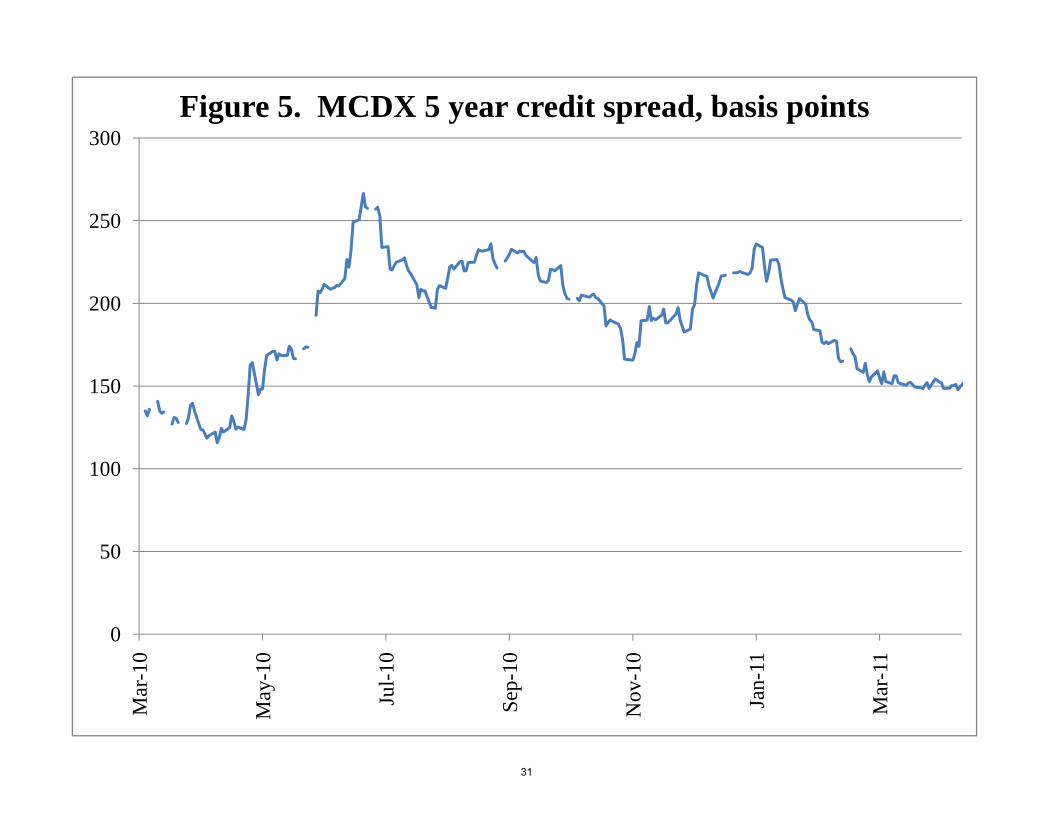
reflect bearish investor sentiment. Figure 5 shows the evolution of the 5-year MCDX municipal credit

spread over the past year. Market prices are already factoring in a disaster scenario. If there is an

aggregate ‘surprise’ in municipal credit markets, it will be on the upside, as the market-forecasted default

rates fail to materialize.

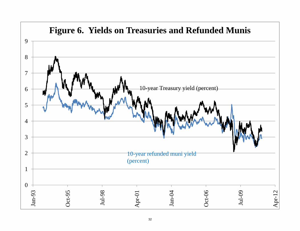
But investor sentiment can push prices out of equilibrium for long periods of time. There are numerous

examples of this phenomenon. One example comes from refunded municipal bonds: these are bonds that

are secured by United States Treasury securities held in escrow. The credit risk of these refunded bonds

is equivalent to the credit risk of Treasuries, and they pay tax-exempt interest. Figure 6 shows yields on

10-year United States Treasury bonds and refunded municipal bonds. The low spread between these

refunded municipal bonds and US Treasuries has been a persistent puzzle, and during the credit crisis the

                                                            15 See New York Times article by Monica Davey, ‘The State that Went Bust,’ January 22, 2011. 16 Based on the following calculation: the December 31, 2010 the MCDX 5-year index spread was 218 basis points. With 70 percent recovery, this spread is consistent with a risk-neutral expectation of 3.63 defaults per year out of the index’s fifty names, or a seven percent default rate. Because defaults frequency is likely correlated with economic downturns, it is reasonable to expect that the risk-neutral probability of municipal default exceeds the physical measure probability of default.

13

spread actually inverted, with the refunded municipal bonds paying a higher pre-tax yield than treasury

bonds. 17 While that obvious anomaly has been reversed, it highlights the potential for prices to remain

out of equilibrium for extended periods of time.

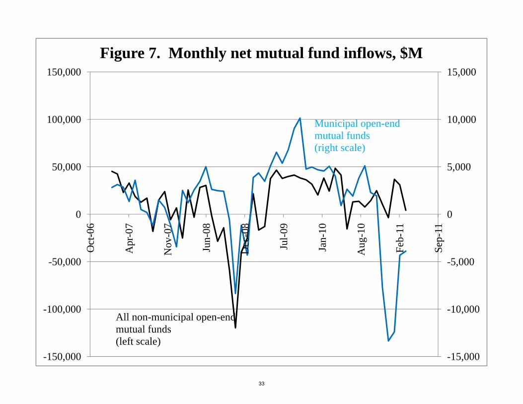
Municipal bonds are largely a retail investment, either held through mutual funds or directly by investors.

Investor flows into municipal mutual funds are an important indicator of investor sentiment, and the

recent signals continue to be bad. Figure 7 shows monthly net inflows and outflows from open-end

mutual funds. The net outflow from municipal bond funds since December of 2010 has totaled more than

$38 Billion.18 These flows can continue to exert a negative influence on municipal bond prices, and

there is no guarantee that spreads will not widen again in the future.

Wagner and Sobel (2006) note that there is some precedent for the loss of an entire class of municipal

investors. The changes in the tax code with the 1986 Tax Reform Act eliminated the tax advantages that

depository institutions had enjoyed in holding municipal debt. Prior to the reform, these institutions had

been able to deduct interest payments on debt used to finance tax-exempt debt, a rule that allowed the

institutions to enjoy a spread between the net return on their municipal investments and the after-tax cost

of their financing. The 1986 tax reform eliminated this practice. At the same time, by reducing the

marginal tax rates at the top of the income distribution, the reform reduced the advantage to holding

municipal debt.

Figure 8 illustrates the results of these changes. The share of municipal debt owned by depository

institutions peaked at over 50 percent in the 1970s, then fell rapidly to under 10 percent, where it remains

today. Most of the drop in the share of debt held by banks and thrifts preceded the formal implementation

of the tax reform rules changes, which were widely anticipated in advance of the law change. The drop in

the share held by depository institutions was accommodated by the household sector and by mutual funds,

which for the most part represent an institutional channel for household investment. So as one considers

the future of the municipal bond market, and the potential for a protracted investor strike, there is some

precedent for the drying up of an entire class of investors in the municipal market.

Depository institutions have not completely left the municipal credit market. The 1986 tax reform created

a specific class of municipal debt, called ‘qualified tax-exempt’ obligations, or ‘bank-qualified’ debt.

Banks can deduct 80 percent of the carrying cost of these obligations from their taxes. Issuers must be

‘qualified small issuers,’ now defined as issuers who sell no more than $30 million of tax-exempt bonds

                                                            17 See also Chalmers (1998). See also Bergstresser, Cohen, and Shenai (2011), which explores a persistent anomaly in the pricing of insured and uninsured municipal debt. 18 The Federal Reserve’s Flow of Funds accounts estimate that open-end mutual funds held in aggregate $532.8 Billion in municipal securities as of September 2010.

14

during the year. In the event of a continuing investor strike, one potential channel of indirect federal

support for the municipal bond market could be to further relax the rules governing bank-qualified debt.19

The decline of the financial guarantors will play an important role in changing the nature of household

investment in municipal bonds. Stable financial guarantors commoditized roughly half of the market, and

allowed relatively uninformed investors to invest based on the credit ratings of the monoline insurers.

With stable guarantors now a thing of the past, the role for active credit management of municipal bond

portfolios has increased.20 This suggests that the locus of household investing in municipal securities will

move from the direct channel to intermediated channels. There will be some bumps in this process, and

the protracted investor strike in the municipal market may reflect the opening stage of a reallocation of

household investment in municipal securities from direct investments in bonds to indirect investments in

professionally managed investment vehicles.

Finally, although some states and localities have been relying on credit markets to finance operating

deficits during the recent crisis, municipalities, in general, rely on credit markets to finance new

investment in infrastructure. This swing in investor sentiment is not likely to cause across-the-board

problems for municipalities rolling over debt of the sort that highly-leveraged financial institutions and

nations have experienced. There will be some municipal defaults, however, and particularly high-profile

municipal defaults could have a prolonged impact on market sentiment. A prolonged municipal bond

investor strike would lead to aging and deteriorating infrastructure. But regardless of investor sentiment,

across-the-board municipal bond default is not likely.

7. What about reduced Recovery Act Federal support for states and localities?

The American Recovery and Reinvestment Act of 2009 (the Recovery Act) provided $282 Billion in

Federal funds for programs administered by states and localities. Although this funding runs from 2009

through 2019, more than half of the funding came in fiscal years 2009 and 2010. Table 7 describes the

intertemporal pattern of funding, by funding type.

                                                            19 This mechanism of federal support would be less directly obvious than the direct payments from the federal government that came with the Build America Bonds program. While political economy can be complicated, it is reasonable to expect that less-obvious subsidies will be favored over more-obvious ones. The 2009 Recovery Act increased the ‘qualified small issuer’ threshold from $10 million of issuance to $30 million. 20 Or more accurately, the active credit management activity is moving from the insurers to mutual funds and other investment vehicles.

15

Many analysts have pointed out that, along with budget cuts, tax increases, and reserve funds, the

Recovery Act funding has helped states and cities so far during the deep recession. One potential

implication is that as Recovery Act funding dries up, states and localities will face severe fiscal

headwinds.

The largest component of Recovery Act support has come through the Federal Medical Assistance

Program (FMAP), which provides matching federal funding for state support for Medicaid spending. A

recent GAO report (GAO, 2010) suggests that this program has helped states maintain Medicaid

eligibility and benefit levels during the current recession, and suggests that the reduction in Federal

support through the Recovery Act may make it difficult for states to sustain these levels of services.

A second component of Recovery Act support funded states’ efforts to restore highways and other roads.

In that sense, the Recovery Act financed infrastructure projects that would otherwise have been deferred.

The Recovery Act also established a State Fiscal Stabilization Fund, targeted at fixing shortfalls in state

support for elementary, secondary, and higher education. Most analysts believe that the withdrawal of

Recovery Act support will increase fiscal stress with respect to public education and increase the depth of

cuts needed to balance budgets.

8. What about the declining credit quality of financial guarantors?

The period between 1980 and 2007 saw rapid growth in the share of municipal bonds that are insured by

third-party financial guarantors. These insurers, often referred to as ‘monoline’ insurers due to their one

business of insuring bonds, insured about half of all new issues by 2007.

The monoline insurers also expanded into insuring structured products based on residential mortgages.

The collapse of that market that started in 2006 left almost all of the financial guarantors in precarious

financial positions. Because these guarantors had previously carried the highest credit ratings, the bonds

that they had insured had carried the highest credit ratings as well. The collapse of the insurers means

now that the credit quality of these municipal bonds is now more directly affected by the credit quality of

the underlying municipal issuers.

The struggles of the bond insurers have been an unfortunate surprise for holders of insured municipal

debt. But these struggles have no impact on the underlying credit quality of municipal issuers, as

described above. The tiny default losses on municipal debt always made the existence of bond insurance

something of a puzzle: when it came to insuring municipal bonds the entire industry was, to a first

16

approximation, insuring against events that never happened. The most important effect of the decline of

the monoline insurers is that credit research will now be performed by the investor (or investment

manager) rather than the monoline insurer.

9. What about proposals that would allow states to file for bankruptcy protection?

In states that allow municipal bankruptcy filings, Chapter 9 of the United States bankruptcy code is

available to localities seeking protection from their creditors. Table 8 describes state rules on Chapter 9

bankruptcy filings. Many states that have statutes covering municipal bankruptcy filings require

distressed municipalities to receive approval before receiving protection. For example, in Connecticut,

the city of Bridgeport was prevented by the Governor from filing for bankruptcy protection.21

Before the introduction of municipal bankruptcy laws in 1934, the main remedy for creditors of a

municipality in default was to petition state courts to compel the municipality to increase taxes. The

introduction of the chapter in federal bankruptcy code specifically focusing on municipalities was a

response to perceived weaknesses in the pre-1934 regime and was designed to alleviate the burden of

destructive creditor competition in situations of municipal distress. A number of differences distinguish

municipal bankruptcy from the more familiar corporate and personal bankruptcy processes. For example,

the municipality enjoys the exclusive right to propose restructuring proposals, and there is no arrangement

available (nor would one make sense) for the liquidation of a municipality.

Municipal bankruptcy filings that involve general obligation debt come in two types. The first type

reflects a sudden investment loss (for example, Orange County, CA in 1994) or a large legal judgment

against a municipality (which has recently occurred in Boise County, ID in 2011, the topic of one of the

case studies at the end of this paper.) In the first type of bankruptcy, bondholders generally suffer

minimal losses. For example, in Orange County, cuts in municipal services and tax increases allowed the

county to pay back bondholders in full. The second type of bankruptcy follows years of ongoing

structural operating deficits (for example Vallejo, CA in 2008, the topic of another case study at the end

of this paper.) This type of bankruptcy filing has been very rare, but in the Vallejo case bondholders are

likely to suffer significant losses.

                                                            21 The New England states apart from Connecticut do not have statutes allowing Chapter 9 filings, and Amdursky and Gillette (1992) note an additional remedy that may be available to bondholders in those states: ‘Execution on Property of Residents…Lest one dismiss the action as an idiosyncracy of a bygone era, it should be recognized that statutes provide for execution against property of a municipal debtor’s constituents in Maine, New Hampshire, and Vermont, and the doctrine has not been rejected in any of the New England jurisdictions where it was once enforced.’   

17

Bankruptcy filings involving general obligation municipal debt have been very rare. Of the 183 Chapter

9 bankruptcy filings since 1980, 113 have been by municipal utilities districts or special municipal

districts. Another 23 have been for hospital or health care authorities. Only 32 have been filings by

cities, villages or counties.22

At the moment there is no provision in the bankruptcy code for a state to file for protection from its

creditors. On February 14, 2011 a House Judiciary Committee subcommittee hearing explored changing

the law to allow states to declare bankruptcy.23 Although the hearing seems to have spooked municipal

markets, the experts who testified appeared to reject the idea of state bankruptcy protection. As James

Spiotto pointed out, ‘Both practical and constitutional considerations mandate the rejection of a State

bankruptcy option.’

Indeed, the impetus for holding hearings exploring state bankruptcy appears not to have come from the

states themselves, who appear to view even the mention of readjustment of debts as a matter that could

create stigma and increase borrowing costs. Again, as Spiotto noted, ‘There is an understandable

leeriness to jump into the uncharted waters of State bankruptcy when the cause of financial difficulty can

be traced to several discrete problems that can be dealt with separately.’

Although municipalities have long-term budget problems, there does not seem to be a broad push coming

from states and cities to expand the bankruptcy option for municipalities. This likely reflects two factors.

First, for most states and localities payments on municipal debt are low enough that the chaos and loss of

control that would follow a municipal bankruptcy filing are not worth the limited benefits that would

follow.

A second factor reflects the political economy of municipal bonds: they are disproportionately held by

within-state high-net-worth individual investors. The pain of municipal default or bankruptcy would not

be felt by far-away institutions. That pain would be felt by people who are close, who are rich, and who

tend to vote. This drives our forecast that most of the pain from any coming fiscal adjustments will be

borne those who rely on state and local services, and not by holders of municipal debt.

10. Municipal crisis case studies

a. Vallejo, CA

                                                            22 See Spiotto, 2008. 23 See http://judiciary.house.gov/hearings/hear_02142011.html.

18

On May 6, 2008, the Vallejo, California City Council voted to file for Chapter 9 bankruptcy. Vallejo is

the largest city in the state to file for bankruptcy protection and is currently the largest city operating

under bankruptcy protection.

On January 18, 2011, Vallejo filed a plan of adjustment with the United States Bankruptcy Court in

Sacramento. The plan is unique in that it proposes paying general unsecured creditors much less than the

full value of their claims. This would be the first time that a city or county under bankruptcy protection

had paid creditors less than the nominal value that they were owed. It remains unclear whether the court

will approve the proposal, but an approval involving partial payments would be a new and potentially

unsettling precedent for municipal credit markets.

Vallejo’s problems stem in part from unusually generous compensation arrangements for city police and

firefighters. Prior to filing for bankruptcy protection, seventy-four percent of the city’s $80 million in

general fund expenditures went towards police and fire salaries. These salaries were based on generous

contracts established following a disruptive police strike during the 1970s. These arrangements combined

with a dramatic reduction in tax collections and a 67 percent drop in city housing values during the

recession to hurt Vallejo’s financial stability.

Vallejo has had a steeper drop in housing values than any of the cities in the Case-Shiller housing index –

higher than the 58 percent peak-trough drop in Las Vegas and the 55 percent peak-trough drop observed

in Phoenix. Vallejo is unusual in its combination of extremely high public employee legacy costs and

housing price drop. Las Vegas and Phoenix, with more recent population growth, do not have quite the

same burden of legacy costs as Vallejo.

Some observers watching Vallejo’s Chapter 9 experience are now expressing the view that other

municipalities are learning from Vallejo that the costs of Chapter 9 outweigh the benefits. According to a

recent Bloomberg article:

When Vallejo, California filed for bankruptcy in 2008 after failing to win union pay cuts,

Councilwoman Stephanie Gomes said officials around the U.S. would have their eyes trained on

the city of 120,000. She was right. The lesson they’ve taken from the two-year old case, which

has cost Vallejo $9.5 million in legal fees and made it a nationwide symbol for distressed

municipal finances, is that out-of-court negotiations yield better results…The Vallejo bankruptcy

resonates in Tracy, a city of about 82,000 residents 60 miles east of San Francisco, said Zane

19

Johnston, the finance director. In the face of a $7.5 million budget gap, the police union agreed to

cancel remaining raises and boost the retirement age to 55 from 50 for new hires.24

At the moment, Vallejo does not appear to be an unambiguous advertisement for municipal Chapter 9

filings.

b. Boise County, ID

Boise County, Idaho is a small, rural county, with about 7,500 residents. It is not home to the mid-sized

city of Boise. The city of Boise is in the county seat of the much larger Ada County, Idaho.

Boise County recently lost a federal lawsuit related to the county’s placement of restrictions on a

developer attempting to construct a residential treatment facility. A federal court ruled that the county’s

restrictions violated the Fair Housing Act and awarded a $5.4 million judgment. This judgment is a large

burden for a county whose annual operating budget is $9.4 billion.

The county filed for bankruptcy protection in March of 2011. The Boise County filing was the first

municipal bankruptcy filing of 2011. In many respects, Boise County represents a smaller example of

earlier cases such as Orange County, California, where a large one-time shock affects the finances of a

county with fundamentally sound fiscal management. In the case of Orange County, bankruptcy

protection was used to prevent the seizure of assets while the county arranged a plan to pay its creditors,

which it eventually did in full through tax increases and spending cuts. The most likely forecast is that

Boise County will do the same – use the bankruptcy protection to arrange a plan for repaying its new

creditor. The county does not have any bonds outstanding.

c. Jefferson County, AL

While the overall liquidity of municipalities is strong, Jefferson, Alabama is an example of a municipality

that has been driven to default by unusually poor liquidity management. Jefferson moved in 2002 away

from fixed-rate debt toward using a combination of variable-rate debt and interest rate swaps. This

transition, at least in retrospect, appears to have been a mistake. This variable-rate debt included Auction-

Rate Securities as well as other types of variable-rate debt.                                                             24 Alison Vekshin and Martin Z. Braun, ‘Vallejo’s Bankruptcy ‘Failure’ scares cities into cutting costs,’ Bloomberg, December 14, 2010. http://www.bloomberg.com/news/2010-12-14/vallejo-s-california-bankruptcy-failure-scares-cities-into-cost-cutting.html.  

20

Auction-Rate securities are long-term securities that pay a floating coupon based on periodic auctions.

These auctions are often held at a monthly or weekly frequency. In the event of a ‘failed auction,’ current

holders of the securities continue to hold the securities and the coupon rate resets to a pre-specified

‘maximum’ rate, often some multiple of LIBOR or some other benchmark rate.25 Failures in the ARS

market were all but unknown until the 2008 liquidity crisis, and the securities were often marketed to

investors as a yield-enhanced cash substitute. Jefferson also used Variable Rated Demand Obligations

(VRDOs), which are distinguished from ARS by the existence of a third-party liquidity provider; in the

event of a failed auction the liquidity provider is obligated to purchase the issuers’ bonds.

A cascading sequence of problems during the 2008 crisis led to widespread auction failures and the

interest rate on Jefferson County’s debt reset from 3 percent to 10 percent. At the same time, because the

bonds were insured by newly-downgraded financial guarantors, the downgrade of the financial guarantors

led to demands from the VRDO liquidity providers that Jefferson County post additional collateral.

Jefferson had also entered into swap contracts to hedge the variable-rate exposure from the VRDO and

ARS securities. This caused two problems: first, the swap contracts failed to perform as expected when

interest rates on municipal variable rate securities diverged from the floating rates on the county’s swap

contracts. Second, the downgrade of Jefferson County led swap counterparties to terminate the swap

contracts and demand additional collateral.

These problems led Jefferson to default on its General Obligation and sewer debt in 2008. An FBI

investigation led to the arrest and subsequent conviction of former Jefferson county commission president

and Birmingham mayor Larry Langford. Langford was found guilty of receiving bribes for influencing

the bond deals related to Jefferson’s liquidity problems and default. He is now serving a 15-year sentence

in federal prison.

On a bond-weighted basis, all kinds of variable-rate financing amounts to about 4.4 percent of municipal

debt currently outstanding. This total includes all kinds of variable-rate financing, ranging from very

simple floating-rate notes to more highly structured instruments like ARS and VRDOs. Weighted by

dollar face value outstanding, the total amounts to 17.3 percent of outstanding municipal debt; variable-

rate bonds tend to be much larger than other types of municipal debt.26 Table 6 shows for each state the

amount of debt issued by all of the issuers in that state, as well as the share of that debt that is maturing

soon and the share of the debt that is variable rate. This table illustrates the heterogeneity in potential

                                                            25 See Bergstresser, Cole, and Shenai, 2009. 26 While there are no good data on aggregate totals, the municipal bond underwriters that I have talked to suggested that about half of variable rate debt is swapped to create a fixed-rate exposure.

21

liquidity problems across states. Wisconsin, although not unusually highly levered, has a significant

share of its debt maturing in the next year. Mississippi has a large share of variable-rate debt. If this debt

is matched with appropriate hedges, the state would be vulnerable to budget problems if there were a

spike in municipal yields

It is possible that other municipalities will turn out to have mismanaged liquidity risk related to variable-

rate financing and interest rate swaps. But the extent of mismanagement and crime in Jefferson County

appears to be unique. The collapse of the ARS market is now three years in the past, and while other

municipalities were adversely affected, Jefferson County remains the only major municipal borrower

forced into default by the turmoil in the variable rate borrowing market.

d. Harrisburg, PA

The crisis in the city of Harrisburg, PA illustrates how a chronic mismanagement and an extreme shock

can push a city into financial distress. The Harrisburg Authority (THA) owns a waste-to-energy trash

incinerator, which it purchased from Harrisburg in 1993. The incinerator was closed in 2003 in order to

comply with orders from the United States Environmental Protection Agency (EPA) and the Pennsylvania

Department of Environmental Protection (DEP). At that point a project to retrofit the incinerator began.

The project ran over-time and over-budget, and was financed with a sequence of revenue bonds issued by

THA.

These bonds for the retrofit project now amounts to approximately $242 million, and debt service

between 2010 and 2034 ranges from $14.6 million to $27.6 million per year. The project has now been

completed, and since 2007 the facility has been operated by the Covanta, a private operator. Operating

profits on the facility are not sufficient to cover maturity debt issued by THA. The revenue bonds have

also been guaranteed by Harrisburg, and most of the debt was secondarily guaranteed by Dauphin

County, of which Harrisburg is the county seat. Assured Guaranty, a relatively stable financial guarantor,

has also underwritten policies insuring THA debt.

Harrisburg also has outstanding General Obligation debt not related to THA debt, and has revenue debt

secured by parking concessions. Harrisburg apparently came close to skipping a payment on its GO debt,

an outcome that was avoided only when the State of Pennsylvania accelerated payments due from the

state to the city. THA bondholders have avoided losses because of the guarantees from the County and

from Assured, both of which have filed suit against Harrisburg.

22

While many observers identify Harrisburg’s guarantee of the THA debt as the source of its financial

difficulties, it is more accurate to say that both the THA guarantee and years of chronic financial

mismanagement are behind the city’s trouble. The Pennsylvania Municipalities Recovery Act (Act 47)

allows a distressed municipality to access professional services and other state support for crafting a

recovery plan; Harrisburg has been operating under Act 47 since December 2010. This is not the same as

a Chapter 9 filing, and does not preclude a Chapter 9 filing in the future. The State, in its approval of

Harrisburg’s request for Act 47 status, notes that budgets had been repeatedly ‘balanced’ only through

one-time sale of assets and issuance of debt. A recent report by Cravath, Swaine, and Moore, which has

been advising Harrisburg during the restructuring, notes that a Chapter 9 filing can be avoided through a

combination of measures, notably including selling off city assets. Their report identifies the THA

facility and parking facilities as the only likely sources of revenue, potentially augmented with the sale of

certain city buildings.

This plan, if followed, seems likely to allow Harrisburg to avoid default during the current recession.

Losses for bondholders will be ameliorated or prevented by the patchwork of guarantees and insurance

policies: Dauphin County, Assured Guaranty, and Ambac (for the Harrisburg GO debt) may suffer losses

if the current distress is not resolved. The case study does raise questions about the longer term. At some

point, Harrisburg will have sold off all of its monetizable assets. Postponement of fiscal adjustments will

make the eventual adjustment very abrupt.

23

11. References

Amdursky, Robert S. and Clayton P. Gillette, 1992, Municipal Debt Finance Law: Theory and Practice, Aspen Publishers, New York.

Baker, Dean, 2011, ‘The origins and severity of the public pension crisis,’ Center for Economic and Policy Research white paper, February 2011.

Barrett, Katherine, and Richard Greene, 2010, ‘State fiscal gimmicks: A budgetary balancing act,’ The American Prospect, 21:2, page A20.

Bennett, James T. and Thomas J. DiLorenzo, 1982, ‘Off-budget activities of local government: The bane of the tax revolt,’ Public Choice 39, pp. 333-342.

Bergstresser, Daniel, Randolph Cohen, and Siddharth Shenai, 2011, ‘Financial guarantors and the 2007-2009 credit crisis,’ working paper, Harvard Business School. Available at http://papers.ssrn.com/sol3/papers.cfm?abstract_id=1571627.

Bergstresser, Daniel, Shawn Cole, and Siddharth Shenai, 2009, ‘UBS and Auction Rate Securities,’ Harvard Business School case.

Brown, Jeffrey R. and David W. Wilcox, 2009, ‘Discounting state and local pension liabilities,’ American Economic Review.

CBS News, 2010, ‘State budgets: The day of reckoning,’ 60 Minutes, December 19, 2010. Accessed at http://www.cbsnews.com/stories/2010/12/19/60minutes/main7166220.shtml?tag=contentMain;contentBody.

Chalmers, John M.R., 1998, ‘Default risk cannot explain the muni puzzle: Evidence from municipal bonds that are secured by U.S. Treasury obligations,’ Review of Financial Studies.

Hou, Yilin, and Daniel L. Smith, 2006, ‘A framework for understanding state balanced budget requirement systems: Reexamining distinctive features and an operational definition,’ Public Budgeting & Finance, pp. 22-45.

International Monetary Fund, 2011, Fiscal Monitor: Shifting gears, tackling challenges on the road to fiscal adjustment. April, 2011.

Munnell, Alicia H., Jean-Pierre Aubry, and Laura Quinby, 2010, ‘The impact of public pensions on state and local budgets,’ Center for Retirement Research white paper #13, Boston College.

National Association of State Budget Officers, 2008, Budget Processes in the States.

National Association of State Budget Officers, 2010, The Fiscal Survey of States.

National Association of State Budget Officers, 2010, 2009 State Expenditure Report.

Novy-Marx, Robert and Joshua Rauh, 2010, ‘Public pension promises: How big are they and what are they worth?,’ working paper, Northwestern University (forthcoming in Journal of Finance).

24

Poterba, James M., 1995, ‘Balanced budget rules and fiscal policy, evidence from the states,’ National Tax Journal, 48:3, pp. 329-336.

United States Government Accounting Office, 1993, ‘Balanced Budget requirements: State experiences and implications for the Federal Government,’ GAO report AFMD-93-58BR.

United States Government Accountability Office, 2010, ‘Recovery Act: One year later, States’ and localities’ uses of funds and opportunities to strengthen accountability,’ GAO report GAO-10-437, March 2010.

25

12. Exhibits

26

Figure 1

27

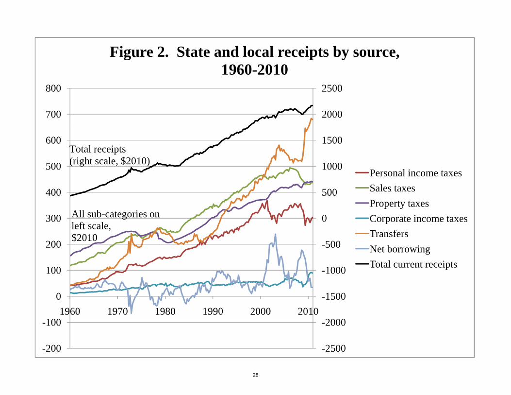
Figure 2. State and local receipts by source, 1960-2010

2000

2500

700

800

1000

1500

500

600

Personal income taxes

Total receipts (right scale, $2010)

0

500

300

400

Personal income taxes

Sales taxes

Property taxes

Corporate income taxesAll sub-categories on

-500

0

200

300 Corporate income taxes

Transfers

Net borrowing

Total current receipts

left scale, $2010

-1500

-1000

0

100

1960 1970 1980 1990 2000 2010

Total current receipts

-2500

-2000

-200

-1001960 1970 1980 1990 2000 2010

28

0.020.5

Figure 3. State and local borrowing, 1947-2010

0.016

0.018

0.4

0.45

0.012

0.014

0.3

0.35 (Debt + Gross pension liability)/GDP(left scale)

0 008

0.01

0 2

0.25

Interest payments/GDP(right scale)

0 004

0.006

0.008

0 1

0.15

0.2

0.002

0.004

0.05

0.1Debt/GDP(left scale)

00

Jun-

45

Jul-

49

Aug

-53

Oct

-57

Nov

-61

Dec

-65

Feb

-70

Mar

-74

Apr

-78

May

-82

Jul-

86

Aug

-90

Sep

-94

Nov

-98

Dec

-02

Jan-

07

Feb

-11

29

120%6%

Figure 4. Municipal debt maturity profile, 2011

100%5%

80%4%

Cumulative percent of debt maturing(right scale)

60%3%

40%2%Annual percent of debt maturing(left scale)

20%1%

( )

0%0%

2010 2015 2020 2025 2030 2035 2040 2045 2050 2055 2060

30

300Figure 5. MCDX 5 year credit spread, basis points

250

200

150

50

100

0

50

Mar

-10

May

-10

Jul-

10

Sep

-10

Nov

-10

Jan-

11

Mar

-11

31

9

Figure 6. Yields on Treasuries and Refunded Munis

7

8

6

7

10-year Treasury yield (percent)

4

5

2

3

10-year refunded muni yield

1

10 year refunded muni yield(percent)

0

Jan-

93

Oct

-95

Jul-

98

Apr

-01

Jan-

04

Oct

-06

Jul-

09

Apr

-12

32

15,000150,000

Figure 7. Monthly net mutual fund inflows, $M

10,000100,000 Municipal open-end

5,00050,000

mutual funds(right scale)

00

6 7 7 8 8 9 0 0 1 1

-5,000-50,000

Oct

-06

Apr

-07

Nov

-07

Jun-

08

Dec

-08

Jul-

09

Jan-

10

Aug

-10

Feb

-11

Sep

-11

-10,000-100,000All non-municipal open-end

-15,000-150,000

All non municipal open endmutual funds(left scale)

33

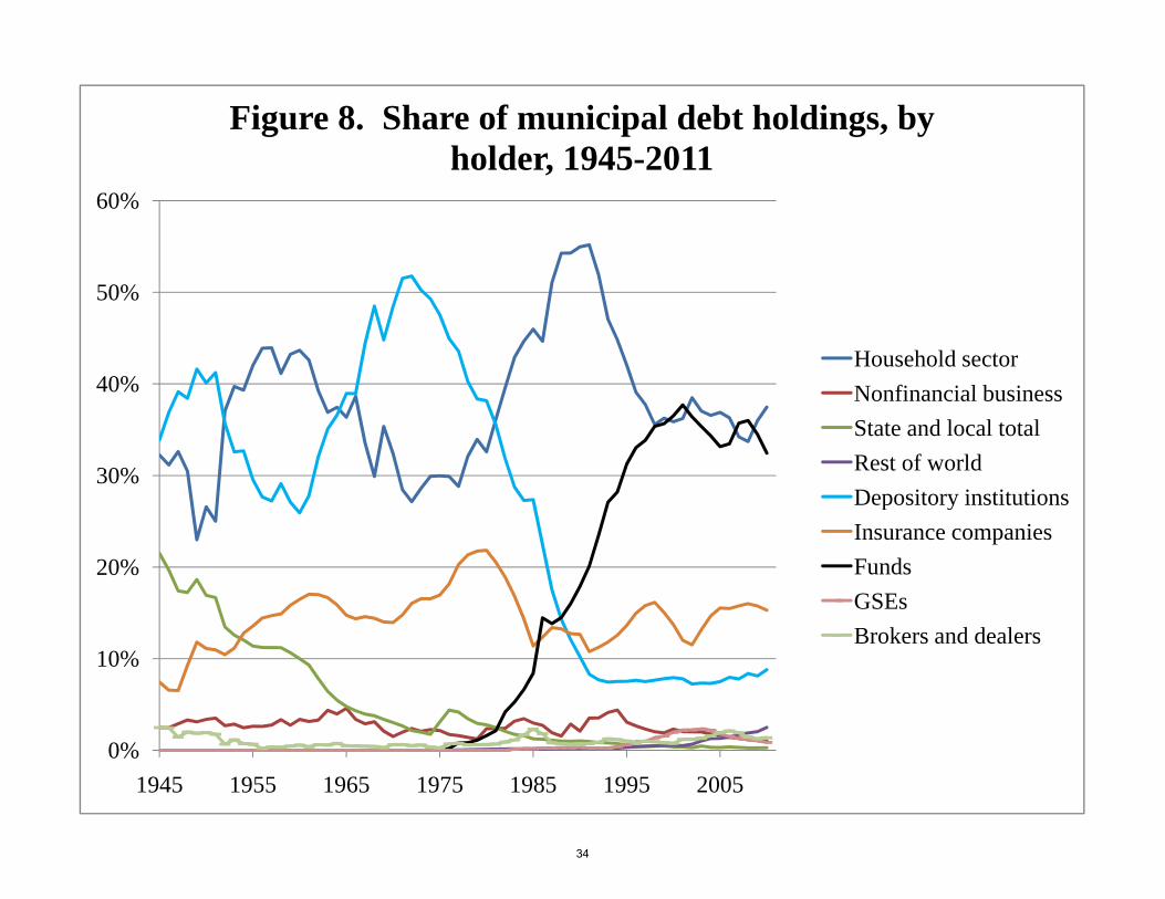
Figure 8. Share of municipal debt holdings, by holder, 1945-2011

50%

60%

40%

50%

Household sector

Nonfinancial business

30%

Nonfinancial business

State and local total

Rest of world

Depository institutions

20%

Depository institutions

Insurance companies

Funds

GSEs

10%

GSEs

Brokers and dealers

0%

1945 1955 1965 1975 1985 1995 2005

34

Table 1. Total receipts of State and Local sector

Period

Personal income

taxesSales taxes

Property taxes

Corp. income

taxes

Transfers (mostly

Federal)Net

borrowingOther

sources

Note: receipts

exc. transfers

2002 Q1 1939.9 312.6 456.8 395.6 39.8 512.7 203.1 19.4 1427.22002 Q2 1942.1 295.0 457.4 399.8 42.0 530.5 204.3 13.1 1411.62002 Q3 1972.8 311.3 462.3 403.3 43.5 534.8 190.0 27.6 1438.02002 Q4 1972.0 310.0 458.1 404.7 45.7 540.0 202.8 10.6 1432.02003 Q1 1929.1 293.3 454.4 401.9 46.2 524.1 238.6 -29.3 1405.02003 Q2 1966.9 280.6 461.4 406.3 42.3 566.0 184.0 26.3 1401.02003 Q3 2014.9 310.9 467.4 409.6 44.6 569.9 157.0 55.6 1445.02003 Q4 2047.0 317.8 472.2 413.8 47.8 580.7 118.6 96.2 1466.32004 Q1 2031.4 314.1 474.3 416.7 49.4 558.9 150.1 67.9 1472.52004 Q2 2040.0 306.7 474.2 418.5 52.7 567.0 153.2 67.6 1473.02004 Q3 2046.7 320.2 471.7 418.4 55.8 557.7 136.2 86.7 1489.02004 Q4 2067.0 329.6 475.6 416.8 55.2 563.2 94.9 131.7 1503.82005 Q1 2083.6 331.9 482.0 417.9 68.1 552.6 74.4 156.7 1531.02005 Q2 2082.4 331.6 485.4 418.1 64.4 549.5 80.7 152.7 1532.82005 Q3 2076.4 331.4 486.5 416.6 63.6 543.4 66.7 168.3 1533.02005 Q4 2081.1 336.1 480.7 415.9 68.2 540.0 95.2 145.0 1541.02006 Q1 2095.9 347.3 493.2 419.5 69.4 523.7 30.6 212.2 1572.22006 Q2 2097.8 350.2 492.4 420.1 69.0 524.7 39.8 201.7 1573.12006 Q3 2090.4 340.8 491.0 423.3 69.9 525.9 61.2 178.4 1564.52006 Q4 2075.9 343.7 489.9 427.7 62.0 512.4 70.2 170.0 1563.52007 Q1 2102.8 355.5 487.9 427.5 65.2 527.9 87.2 151.6 1574.92007 Q2 2094.1 354.2 486.8 428.9 64.6 527.6 80.6 151.6 1566.52007 Q3 2074.6 348.2 483.1 429.9 60.5 524.9 97.9 130.2 1549.82007 Q4 2054.1 341.2 477.8 427.9 60.0 519.9 136.0 91.3 1534.22008 Q1 2036.8 351.1 466.1 423.4 52.4 521.9 144.1 77.8 1514.92008 Q2 2031.4 355.4 455.5 419.2 53.3 522.3 149.5 76.2 1509.12008 Q3 1998.4 336.7 449.1 417.4 54.8 518.4 177.3 44.7 1480.02008 Q4 1996.8 331.9 444.2 427.4 36.1 538.7 172.5 45.9 1458.02009 Q1 2030.4 310.6 439.5 435.0 44.5 584.8 155.0 61.0 1445.62009 Q2 2045.5 272.6 429.3 436.7 45.7 646.3 143.5 71.5 1399.22009 Q3 2073.1 298.0 433.0 438.6 50.1 634.6 112.3 106.5 1438.52009 Q4 2103.5 300.8 430.9 439.2 62.8 645.0 67.5 157.5 1458.62010 Q1 2121.9 295.1 429.7 437.2 83.0 653.9 58.4 164.5 1468.02010 Q2 2129.9 283.5 430.8 439.3 89.0 666.6 69.1 151.5 1463.22010 Q3 2163.6 294.6 436.2 442.1 92.0 683.4 34.3 180.9 1480.22010 Q4 2165.9 303.0 436.8 440.7 89.1 679.4 33.9 183.0 1486.5

Total current

receipts, $2010

Receipts by type, $2010

Source: National Income and Product Accounts, Bureau of Economic Analysis, United States Census Department. Implicit GDP deflator for State and Local government sector used to convert nominal totals to constant 2010 dollars. All figures are seasonally adjusted totals, expressed at annual rates.

35

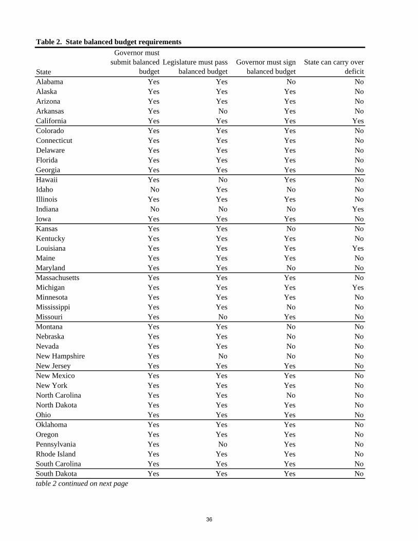
Table 2. State balanced budget requirements

State

Governor must submit balanced

budgetLegislature must pass

balanced budgetGovernor must sign

balanced budgetState can carry over

deficitAlabama Yes Yes No NoAlaska Yes Yes Yes NoArizona Yes Yes Yes NoArkansas Yes No Yes NoCalifornia Yes Yes Yes YesColorado Yes Yes Yes NoConnecticut Yes Yes Yes NoDelaware Yes Yes Yes NoFlorida Yes Yes Yes NoGeorgia Yes Yes Yes NoHawaii Yes No Yes NoIdaho No Yes No NoIllinois Yes Yes Yes NoIndiana No No No YesIowa Yes Yes Yes NoKansas Yes Yes No NoKentucky Yes Yes Yes NoLouisiana Yes Yes Yes YesMaine Yes Yes Yes NoMaryland Yes Yes No NoMassachusetts Yes Yes Yes NoMichigan Yes Yes Yes YesMinnesota Yes Yes Yes NoMississippi Yes Yes No NoMissouri Yes No Yes NoMontana Yes Yes No NoNebraska Yes Yes No NoNevada Yes Yes No NoNew Hampshire Yes No No NoNew Jersey Yes Yes Yes NoNew Mexico Yes Yes Yes NoNew York Yes Yes Yes NoNorth Carolina Yes Yes No NoNorth Dakota Yes Yes Yes NoOhio Yes Yes Yes NoOklahoma Yes Yes Yes NoOregon Yes Yes Yes NoPennsylvania Yes No Yes NoRhode Island Yes Yes Yes NoSouth Carolina Yes Yes Yes NoSouth Dakota Yes Yes Yes Notable 2 continued on next page

36

table 2 continued from previous page

State

Governor must submit balanced

budgetLegislature must pass

balanced budgetGovernor must sign

balanced budgetState can carry over

deficitTennessee Yes Yes Yes NoTexas No Yes Yes NoUtah Yes Yes Yes NoVermont No No No YesVirginia No No Yes NoWashington Yes No No YesWest Virginia No Yes Yes NoWisconsin Yes Yes Yes YesWyoming Yes Yes Yes NoSource: NASBO Budget Processes in the States, 2008

37

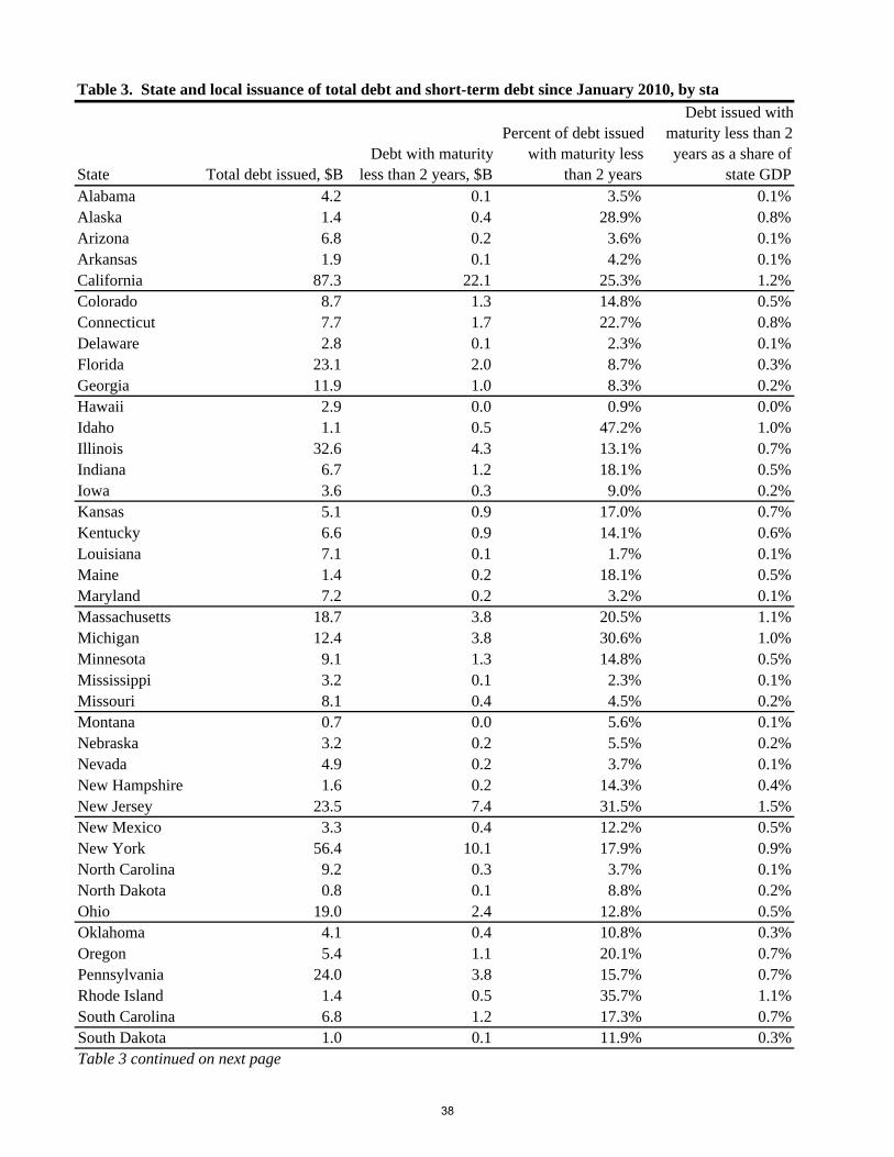
Table 3. State and local issuance of total debt and short-term debt since January 2010, by stat

State Total debt issued, $BDebt with maturity

less than 2 years, $B

Percent of debt issuedwith maturity less

than 2 years

Debt issued withmaturity less than 2 years as a share of

state GDPAlabama 4.2 0.1 3.5% 0.1%Alaska 1.4 0.4 28.9% 0.8%Arizona 6.8 0.2 3.6% 0.1%Arkansas 1.9 0.1 4.2% 0.1%California 87.3 22.1 25.3% 1.2%Colorado 8.7 1.3 14.8% 0.5%Connecticut 7.7 1.7 22.7% 0.8%Delaware 2.8 0.1 2.3% 0.1%Florida 23.1 2.0 8.7% 0.3%Georgia 11.9 1.0 8.3% 0.2%Hawaii 2.9 0.0 0.9% 0.0%Idaho 1.1 0.5 47.2% 1.0%Illinois 32.6 4.3 13.1% 0.7%Indiana 6.7 1.2 18.1% 0.5%Iowa 3.6 0.3 9.0% 0.2%Kansas 5.1 0.9 17.0% 0.7%Kentucky 6.6 0.9 14.1% 0.6%Louisiana 7.1 0.1 1.7% 0.1%Maine 1.4 0.2 18.1% 0.5%Maryland 7.2 0.2 3.2% 0.1%Massachusetts 18.7 3.8 20.5% 1.1%Michigan 12.4 3.8 30.6% 1.0%Minnesota 9.1 1.3 14.8% 0.5%Mississippi 3.2 0.1 2.3% 0.1%Missouri 8.1 0.4 4.5% 0.2%Montana 0.7 0.0 5.6% 0.1%Nebraska 3.2 0.2 5.5% 0.2%Nevada 4.9 0.2 3.7% 0.1%New Hampshire 1.6 0.2 14.3% 0.4%New Jersey 23.5 7.4 31.5% 1.5%New Mexico 3.3 0.4 12.2% 0.5%New York 56.4 10.1 17.9% 0.9%North Carolina 9.2 0.3 3.7% 0.1%North Dakota 0.8 0.1 8.8% 0.2%Ohio 19.0 2.4 12.8% 0.5%Oklahoma 4.1 0.4 10.8% 0.3%Oregon 5.4 1.1 20.1% 0.7%Pennsylvania 24.0 3.8 15.7% 0.7%Rhode Island 1.4 0.5 35.7% 1.1%South Carolina 6.8 1.2 17.3% 0.7%South Dakota 1.0 0.1 11.9% 0.3%Table 3 continued on next page

38

Table 3 continued from previous page

State Total debt issued, $BDebt with maturity

less than 2 years, $B

Percent of debt issuedwith maturity less

than 2 years

Debt issued withmaturity less than 2 years as a share of

state GDPTennessee 6.6 0.3 5.0% 0.1%Texas 49.1 9.9 20.2% 0.9%Utah 4.0 0.3 7.7% 0.3%Vermont 0.7 0.0 6.8% 0.2%Virginia 8.8 0.4 4.9% 0.1%Washington 16.3 0.6 3.7% 0.2%West Virginia 0.8 0.0 3.8% 0.0%Wisconsin 8.7 2.4 27.6% 1.0%Wyoming 0.4 0.0 4.7% 0.1%

Source: State GDP data from US Census Department. Municipal bond issuance data from Mergent.

39

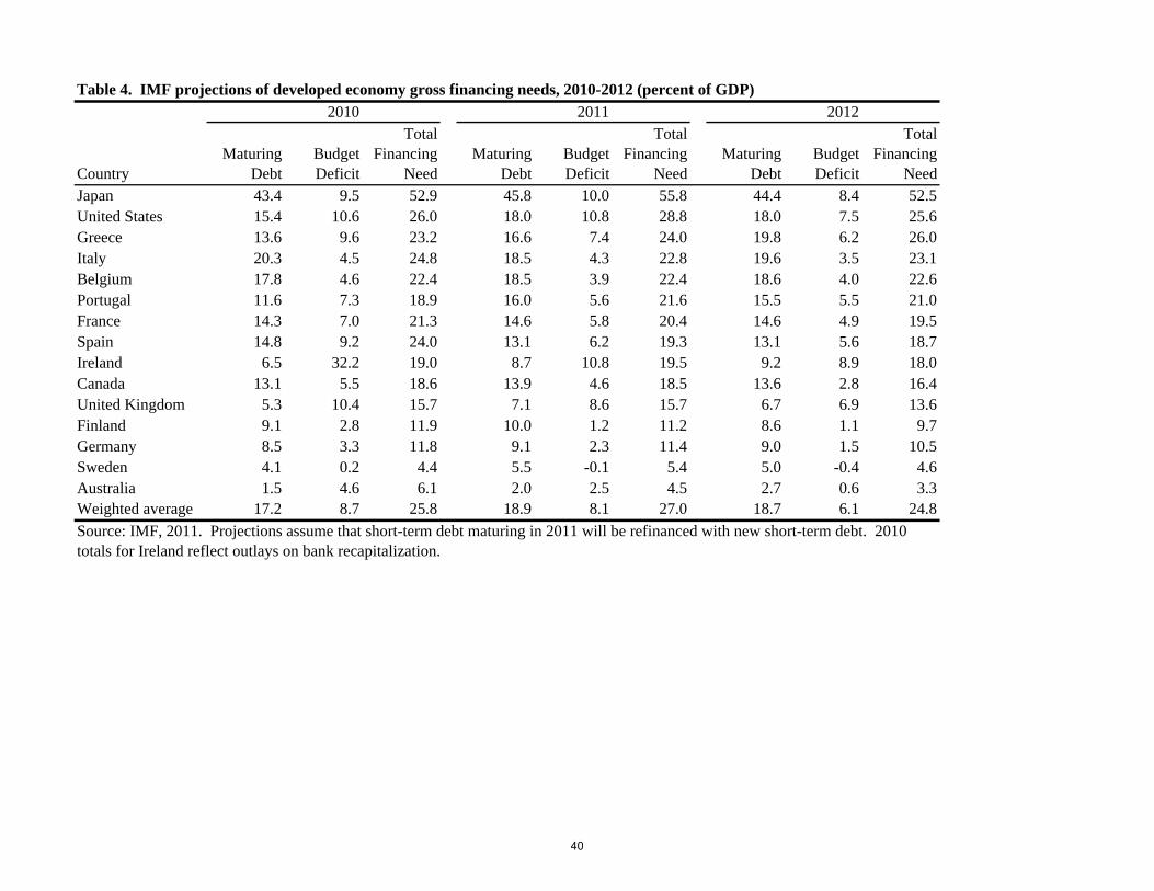
Table 4. IMF projections of developed economy gross financing needs, 2010-2012 (percent of GDP)

2010 2011 2012

CountryMaturing

DebtBudget Deficit

Total Financing

NeedMaturing

DebtBudget Deficit

Total Financing

NeedMaturing

DebtBudget Deficit

Total Financing

NeedJapan 43.4 9.5 52.9 45.8 10.0 55.8 44.4 8.4 52.5United States 15.4 10.6 26.0 18.0 10.8 28.8 18.0 7.5 25.6Greece 13.6 9.6 23.2 16.6 7.4 24.0 19.8 6.2 26.0Italy 20.3 4.5 24.8 18.5 4.3 22.8 19.6 3.5 23.1Belgium 17.8 4.6 22.4 18.5 3.9 22.4 18.6 4.0 22.6Portugal 11.6 7.3 18.9 16.0 5.6 21.6 15.5 5.5 21.0France 14.3 7.0 21.3 14.6 5.8 20.4 14.6 4.9 19.5Spain 14.8 9.2 24.0 13.1 6.2 19.3 13.1 5.6 18.7Ireland 6.5 32.2 19.0 8.7 10.8 19.5 9.2 8.9 18.0Canada 13.1 5.5 18.6 13.9 4.6 18.5 13.6 2.8 16.4United Kingdom 5.3 10.4 15.7 7.1 8.6 15.7 6.7 6.9 13.6Finland 9.1 2.8 11.9 10.0 1.2 11.2 8.6 1.1 9.7Germany 8.5 3.3 11.8 9.1 2.3 11.4 9.0 1.5 10.5Sweden 4.1 0.2 4.4 5.5 -0.1 5.4 5.0 -0.4 4.6Australia 1.5 4.6 6.1 2.0 2.5 4.5 2.7 0.6 3.3Weighted average 17.2 8.7 25.8 18.9 8.1 27.0 18.7 6.1 24.8

Source: IMF, 2011. Projections assume that short-term debt maturing in 2011 will be refinanced with new short-term debt. 2010 totals for Ireland reflect outlays on bank recapitalization.

40

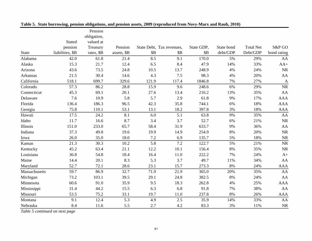
Table 5. State borrowing, pension obligations, and pension assets, 2009 (reproduced from Novy-Marx and Rauh, 2010)

State

Stated pension

liabilities, $B

Pension obligation,

valued at Treasury rates, $B

Pension assets, $B

State Debt, $B

Tax revenues, $B

State GDP, $B

State bond debt/GDP

Total Net Debt/GDP

S&P GO bond rating

Alabama 42.0 61.8 21.4 8.5 9.1 170.0 5% 29% AAAlaska 15.3 21.7 12.4 6.5 8.4 47.9 14% 33% AA+Arizona 43.6 73.5 24.8 10.5 13.7 248.9 4% 24% NRArkansas 21.5 30.4 14.6 4.3 7.5 98.3 4% 20% AACalifornia 518.1 699.7 329.6 121.9 117.4 1846.8 7% 27% AColorado 57.3 86.2 28.8 15.9 9.6 248.6 6% 29% NRConnecticut 45.3 69.1 20.1 27.6 13.4 216.2 13% 35% AADelaware 7.6 10.9 5.8 5.7 2.9 61.8 9% 17% AAAFlorida 136.4 186.3 96.5 42.3 35.8 744.1 6% 18% AAAGeorgia 75.8 110.1 53.1 13.1 18.2 397.8 3% 18% AAAHawaii 17.5 24.2 8.1 6.0 5.1 63.8 9% 35% AAIdaho 11.7 16.6 8.7 3.4 3.7 52.7 6% 21% NRIllinois 151.0 233.0 65.7 58.4 31.9 633.7 9% 36% AAIndiana 37.3 49.8 19.6 19.9 14.9 254.9 8% 20% NRIowa 26.0 35.0 18.0 7.2 6.9 135.7 5% 18% NRKansas 21.3 30.3 10.2 5.8 7.2 122.7 5% 21% NRKentucky 45.2 63.4 21.1 12.2 10.1 156.4 8% 35% NRLouisiana 36.8 54.8 18.4 16.4 11.0 222.2 7% 24% A+Maine 14.4 20.1 8.3 5.3 3.7 49.7 11% 34% AAMaryland 52.7 72.1 28.6 23.1 15.7 273.3 8% 24% AAAMassachusetts 59.7 86.9 32.7 71.9 21.9 365.0 20% 35% AAMichigan 73.2 103.1 39.5 29.1 24.8 382.5 8% 24% AAMinnesota 60.6 91.0 35.9 9.5 18.3 262.8 4% 25% AAAMississippi 31.4 44.2 15.5 6.3 6.8 91.8 7% 38% AAMissouri 53.5 75.2 33.1 19.7 11.0 237.8 8% 26% AAAMontana 9.1 12.4 5.3 4.9 2.5 35.9 14% 33% AANebraska 8.4 11.6 5.5 2.7 4.2 83.3 3% 11% NRTable 5 continued on next page

41

Table 5 continued from previous page

State

Stated pension

liabilities, $B

Pension obligation,

valued at Treasury rates, $B

Pension assets, $B

State Debt, $B

Tax revenues, $B

State GDP, $B

State bond debt/GDP

Total Net Debt/GDP

S&P GO bond rating

Nevada 25.4 36.3 18.8 4.2 6.1 131.2 3% 17% AA+New Hampshire 8.5 12.5 4.3 7.9 2.3 60.0 13% 27% AANew Jersey 132.8 191.2 67.2 52.8 30.6 474.9 11% 37% AANew Mexico 28.8 39.8 15.9 7.8 5.6 79.9 10% 40% AA+New York 239.8 325.7 192.8 114.2 65.4 1144.5 10% 22% AANorth Carolina 74.9 101.8 64.0 19.6 22.8 400.2 5% 14% AAANorth Dakota 4.4 6.3 2.7 2.0 2.3 31.2 6% 18% NROhio 197.5 281.4 114.7 26.9 26.4 471.5 6% 41% AA+Oklahoma 33.6 45.9 15.8 9.1 8.5 146.4 6% 27% AA+Oregon 57.5 80.7 42.9 11.6 7.3 161.6 7% 31% AAPennsylvania 110.6 164.5 64.3 40.7 32.1 553.3 7% 25% AARhode Island 13.9 20.5 6.6 8.9 2.8 47.4 19% 48% AASouth Carolina 42.4 63.5 20.3 15.2 8.5 156.4 10% 37% AA+South Dakota 7.4 10.3 5.6 3.4 1.3 37.0 9% 22% NRTennessee 36.7 49.6 26.4 4.4 11.5 252.1 2% 11% AA+Texas 191.2 268.4 126.1 33.3 44.7 1223.5 3% 14% AAUtah 22.6 31.2 14.7 5.9 5.9 109.8 5% 20% AAAVermont 4.0 5.7 2.4 3.4 2.5 25.4 13% 26% AA+Virginia 69.1 89.6 41.3 21.9 18.4 397.0 6% 18% AAAWashington 62.3 86.4 43.5 23.5 17.9 322.8 7% 21% AA+West Virginia 13.7 18.3 7.2 6.4 4.9 61.7 10% 28% AAWisconsin 79.7 114.6 58.4 22.1 15.1 240.4 9% 33% AAWyoming 7.0 9.8 4.4 1.3 2.2 35.3 4% 19% NRTOTAL 3136.8 4427.4 1941.6 1004.8 780.7 14068.3 7% 25%

42

Table 6. Maturity structure of debt, by state

State Debt/GDP 2011 2011-2 2011-5 Var. rateCalifornia 590.00 1883.65 31.3% 5.4% 7.8% 17.1% 12.8%Texas 317.00 1141.04 27.8% 5.6% 8.6% 18.7% 14.0%New York 394.00 1084.26 36.3% 4.9% 9.3% 21.8% 17.7%Florida 187.00 729.96 25.6% 5.3% 10.4% 21.3% 20.5%Illinois 188.00 621.31 30.3% 5.0% 8.4% 20.8% 15.3%Pennsylvania 163.00 547.75 29.8% 4.9% 8.3% 18.8% 22.6%New Jersey 150.00 479.50 31.3% 6.9% 10.3% 21.2% 9.1%Ohio 111.00 465.83 23.8% 4.1% 7.2% 17.9% 18.8%Virginia 74.90 406.25 18.4% 3.9% 7.8% 19.7% 16.0%North Carolina 64.20 398.66 16.1% 3.7% 7.6% 20.3% 23.9%Georgia 78.30 393.47 19.9% 4.3% 8.7% 19.7% 18.4%Massachusetts 109.00 362.89 30.0% 5.7% 9.7% 21.4% 19.3%Michigan 95.10 361.25 26.3% 5.8% 9.3% 20.2% 18.5%Washington 93.50 336.24 27.8% 3.4% 7.7% 20.2% 11.4%Maryland 52.10 283.54 18.4% 4.1% 8.5% 22.4% 15.8%Minnesota 56.30 257.63 21.9% 6.5% 11.5% 26.2% 14.1%Indiana 67.10 257.43 26.1% 4.2% 9.6% 27.1% 18.7%Arizona 63.00 254.16 24.8% 5.2% 9.3% 21.8% 12.9%Colorado 69.70 250.83 27.8% 3.9% 7.0% 16.4% 19.3%Tennessee 49.40 241.77 20.4% 3.5% 7.4% 19.5% 28.5%Wisconsin 51.20 238.99 21.4% 8.2% 13.2% 29.0% 17.2%Missouri 60.00 236.91 25.3% 2.6% 5.1% 14.0% 29.1%Connecticut 48.70 220.44 22.1% 7.6% 12.8% 28.3% 11.9%Louisiana 42.50 208.59 20.4% 2.8% 6.2% 17.5% 23.2%Alabama 38.80 168.22 23.1% 2.6% 5.6% 15.1% 27.9%Oregon 38.90 165.24 23.5% 5.9% 9.9% 21.4% 12.7%South Carolina 43.70 158.07 27.6% 4.9% 8.6% 20.2% 20.3%Kentucky 38.50 154.56 24.9% 5.2% 8.7% 19.5% 23.1%Oklahoma 24.80 154.31 16.1% 5.7% 11.4% 25.6% 20.4%Iowa 22.10 136.14 16.2% 5.0% 9.9% 23.9% 23.1%Nevada 33.90 125.23 27.1% 3.5% 7.6% 18.1% 15.4%Kansas 32.90 123.27 26.7% 5.6% 10.4% 26.0% 12.0%Utah 25.40 112.84 22.5% 3.8% 7.6% 20.8% 25.7%Arkansas 10.80 101.19 10.7% 4.1% 7.8% 20.3% 10.6%Mississippi 22.90 95.09 24.1% 3.1% 6.3% 16.7% 36.4%Nebraska 19.20 84.57 22.7% 3.8% 8.2% 24.7% 15.7%New Mexico 18.50 74.33 24.9% 6.0% 10.5% 24.3% 21.5%Hawaii 17.70 65.78 26.9% 3.6% 8.1% 22.6% 5.8%West Virginia 8.09 62.23 13.0% 2.7% 5.7% 15.6% 31.1%Delaware 16.40 59.34 27.6% 2.8% 7.4% 16.9% 34.7%New Hampshire 12.50 59.02 21.2% 2.8% 5.6% 15.9% 27.8%Idaho 7.87 53.52 14.7% 8.9% 11.6% 20.9% 21.9%Table 6 continued on next page

Debt/GDP, by maturity and typeTotal Debt, $B

State GDP (2008), $B

43

Table 6 continued from previous page

State Debt/GDP 2011 2011-2 2011-5 Var. rateMaine 9.20 50.62 18.2% 5.9% 11.3% 26.7% 17.1%Rhode Island 11.70 47.73 24.5% 6.7% 10.2% 22.1% 16.1%Alaska 12.90 46.57 27.7% 4.4% 8.8% 20.4% 25.3%South Dakota 5.94 38.75 15.3% 4.4% 8.1% 17.7% 21.5%Wyoming 5.63 37.47 15.0% 1.5% 2.9% 14.9% 50.4%Montana 6.70 35.60 18.8% 2.1% 4.3% 15.6% 40.7%North Dakota 4.71 31.66 14.9% 4.5% 9.1% 23.2% 13.8%Vermont 7.19 25.12 28.6% 2.7% 6.7% 16.6% 49.7%Sum 3671.93 13928.81 26.4% 5.0% 8.7% 20.1% 17.3%

Source: Mergent. Debt includes all debt issued by both state and local issuers.

Total Debt, $B

State GDP (2008), $B

Debt/GDP, by maturity and type

44

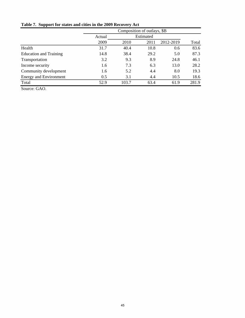
Table 7. Support for states and cities in the 2009 Recovery Act

Actual2009 2010 2011 2012-2019 Total

Health 31.7 40.4 10.8 0.6 83.6Education and Training 14.8 38.4 29.2 5.0 87.3Transportation 3.2 9.3 8.9 24.8 46.1Income security 1.6 7.3 6.3 13.0 28.2Community development 1.6 5.2 4.4 8.0 19.3Energy and Environment 0.5 3.1 4.4 10.5 18.6Total 52.9 103.7 63.4 61.9 281.9

Source: GAO.

EstimatedComposition of outlays, $B

45

Table 8. State statutes covering municipal bankruptcy filings

State

Chapter 9 filings addressed in state statutes? Authorization type Notes

Alabama Yes Specific authorizationAlaska NoArizona Yes Specific authorizationArkansas Yes Specific authorizationCalifornia Yes Specific authorizationColorado Yes* *Authorization for irrigation

and drainage districts.Connecticut Yes Conditional No authorization without

express, written consent of Governor.

Delaware NoFlorida Yes Specific authorizationGeorgia Yes Bankruptcy specifically

prohibited by statuteHawaii NoIdaho Yes Specific authorizationIllinois Yes Conditional Allowed if a Financial

Planning Board is created and judges that bankruptcy is in the municipality's interest.

Indiana NoIowa Yes Conditional Allowed only if the

municipality is insolvent as a result of involuntary debt.

Kansas NoKentucky Yes Conditional County must receive approval

from state local debt officer and state local finance officer in order to declare bankruptcy.

Louisiana Yes Conditional Need approval from State Bond Commission, Governor, and Attorney General.

Maine NoMaryland NoMassachusetts NoMichigan Yes Conditional Multiple review processes.Table 8 continued on next page

46

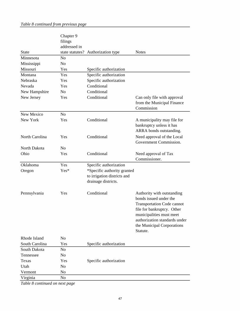
State

Chapter 9 filings addressed in state statutes? Authorization type Notes

Minnesota NoMississippi NoMissouri Yes Specific authorizationMontana Yes Specific authorizationNebraska Yes Specific authorizationNevada Yes ConditionalNew Hampshire No ConditionalNew Jersey Yes Conditional Can only file with approval

from the Municipal Finance Commission

New Mexico NoNew York Yes Conditional A municipality may file for

bankruptcy unless it has ARRA bonds outstanding.

North Carolina Yes Conditional Need approval of the Local Government Commission.

North Dakota NoOhio Yes Conditional Need approval of Tax

Commissioner.Oklahoma Yes Specific authorizationOregon Yes* *Specific authority granted

to irrigation districts and drainage districts.

Pennsylvania Yes Conditional Authority with outstanding bonds issued under the Transportation Code cannot file for bankruptcy. Other municipalities must meet authorization standards under the Municipal Corporations Statute.

Rhode Island NoSouth Carolina Yes Specific authorizationSouth Dakota NoTennessee NoTexas Yes Specific authorizationUtah NoVermont NoVirginia No

Table 8 continued from previous page

Table 8 continued on next page

47

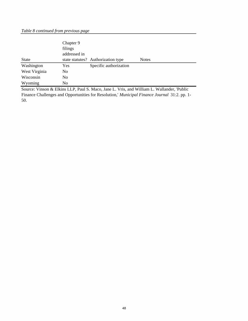
State

Chapter 9 filings addressed in state statutes? Authorization type Notes

Washington Yes Specific authorizationWest Virginia NoWisconsin NoWyoming NoSource: Vinson & Elkins LLP, Paul S. Maco, Jane L. Vris, and William L. Wallander, 'Public Finance Challenges and Opportunities for Resolution,' Municipal Finance Journal 31:2. pp. 1-50.

Table 8 continued from previous page

48