Hastings Law Journal

Volume 59 | Issue 5 Article 10

1-2008

Why Binomial Distributions Do Not Work asProof of Employment DiscriminationBen Ikuta

Follow this and additional works at: https://repository.uchastings.edu/hastings_law_journal

Part of the Law Commons

This Note is brought to you for free and open access by the Law Journals at UC Hastings Scholarship Repository. It has been accepted for inclusion inHastings Law Journal by an authorized editor of UC Hastings Scholarship Repository. For more information, please contactwangangela@uchastings.edu.

Recommended CitationBen Ikuta, Why Binomial Distributions Do Not Work as Proof of Employment Discrimination, 59 Hastings L.J. 1235 (2008).Available at: https://repository.uchastings.edu/hastings_law_journal/vol59/iss5/10

Why Binomial Distributions Do Not Work asProof of Employment Discrimination

BEN IKUTA*

INTRODUCTION

In employment discrimination cases under Title VII,' "[n]o issue hasbeen more stubborn than deciding to what extent a plaintiff must presentspecific evidence about a defendant's state of mind."2 Many times, anemployer's violation of Title VII affects the discriminated class as awhole, not just the protected individual.3 The plaintiff in these "systemicdisparate treatment" cases must prove the elements of a prima facie case,which requires that he or she presents a set of facts that raise "aninference of discrimination . . . because these acts, if otherwiseunexplained, are more likely than not based on the consideration ofimpermissible factors."4 However, contrary to individual disparatetreatment cases,5 specific and isolated proof of discrimination is usuallynot sufficient in systemic disparate treatment cases to show a prima faciecase since discrimination must be "the [defendant's] standard operatingprocedure-the regular rather than the unusual practice."' Additionally,

* J.D., University of California, Hastings College of the Law, 2008. I would like to thankJennifer Luczkowiak, Pilar Stillwater, Erik Christensen, Jay Nelson, Katie Annand, Scott Dommes,and Amber Jones for their invaluable assistance on this Note.

i. Title VII prohibits discrimination by employers on the basis of race, color, religion, sex, ornational origin. See 42 U.S.C. § 20ooe (2000). There are also other ways to unlawfully discriminate.E.g., The Age Discrimination in Employment Act, 29 U.S.C. §§ 621-34.

2. ROBERT N. COVINGTON & KURT H. DECKER, INDIVIDUAL EMPLOYEE RIGHTS 159 (995).3. THOMAS R. HAGGARD, UNDERSTANDING EMPLOYMENT DISCRIMINATION 83 (2001).

4. Furnco Constr. Corp. v. Waters, 438 U.S. 567, 577 (1978). This Note will focus on statisticalanalysis in systemic disparate treatment cases, not systemic disparate impact cases. See Elaine W.Shoben, Differential Pass-Fail Rates in Employment Testing: Statistical Proof Under Title VII, 91 HARV.

L. REV. 793 (1978), for a good description of statistical analysis in systemic disparate impact cases.5. Proof of a prima facie case in individual disparate treatment cases involves four distinct

factors:

(i) that [the applicant] belongs to a [] minority; (ii) that he applied and was qualified for ajob for which the employer was seeking applicants; (iii) that, despite his qualifications, hewas rejected; and (iv) that, after his rejection, the position remained open and the employercontinued to seek applicants from persons of complainant's qualifications.

McDonnell Douglas v. Green, 411 U.S. 792, 802 (973).6. Int'l Bhd. of Teamsters v. United States, 431 U.S. 324, 336 (1977); see also RAMONA L.

[1235]

HASTINGS LAW JOURNAL

not only are individual acts of discrimination insufficient, but"[ajnecdotal evidence of individual class members is not necessary."' Inthese cases, an illustration of a general trend toward discrimination isneeded to establish a prima facie case while individual evidence ofdiscrimination is used only as secondary or persuasive weight, if at all.'

Although it is possible for employer discrimination policies to befacially apparent,9 usually employer policies are not overtlydiscriminatory.'" In those situations where it is not apparent, the onlymethod of proving a prima facie case of discrimination in most systemicdisparate treatment instances is to show a pattern of discrimination in theemployer's hiring decisions." Since these patterns can usually "beidentified and analyzed in quantitative form,"'2 cases rely primarily, andoften exclusively, on statistics.'3 If the plaintiff offers statistics thatindicate a hiring practice that is unlikely absent discrimination, then theplaintiff is deemed to have created a prima facie case, thereby shifting tothe defendant the burden of rebutting the plaintiff's statistical proof.'4

The defendant can rebut this presumption by: (i) demonstrating that theplaintiff's statistics are "inaccurate or insignificant";'5 (2) offering his ownstatistical proof of nondiscriminatory hiring practices; 6 or (3) offering

PAETZOLD & STEVEN L. WILLBORN, THE STATISTICS OF DISCRIMINATION: USING STATISTICAL EVIDENCE IN

DISCRIMINATION CASES I (1994) (illustrating that individual acts of discrimination "[are] not enough tomeet this standard").

7. ROBERT BELTON, REMEDIES IN EMPLOYMENT DISCRIMINATION LAW 49 n.89 (1992); accordPAETZOLD & WILLBORN, supra note 6; MARK A. ROTHSTEIN & LANCE LIEBMAN, EMPLOYMENT LAW:

CASES AND MATERIALS 154 (6th ed. 2007). "Some cases have indicated that statistics alone can create aprima facie case of intentional group exclusion." Id.; see also, e.g., EEOC v. Am. Nat'l Bank, 652 F.2d1176, 1190 (4th Cir. 198i); United States v. Sheet Metal Workers Int'l Ass'n Local 36, 416 F.2d 123,127 n.7 (8th Cir. 1969).

8. BELTON, supra note 7, at 49.9. E.g., L.A. Dep't of Water & Power v. Manhart, 435 U.S. 702, 702 (1978) (requiring female

employees to make larger contributions to the pension fund than male employees).1o. RICHARD R. CARLSON, EMPLOYMENT LAW I 14 (2005) ("[D]iscrimination frequently takes

subtle forms. An employer who knows discrimination is illegal is not likely to announce his bias as amatter of corporate policy. Moreover, bias might affect one supervisor or manager but not others, sothat the effect of the bias is not reflected in overall employment statistics for the entire company.");MACK A. PLAYER, EMPLOYMENT DISCRIMINATION LAW 343 (1988) ("The plaintiff may find 'smoking gun'evidence, such as a written memorandum describing the [discriminatory] policy, but this is notlikely.").

iI. See HAGGARD, supra note 3; PAETZOLD & WILLBORN, supra note 6; Louis J. Braun, Statisticsand the Law: Hypothesis Testing and Its Application to Title VII Cases, 32 HASTINGS L.J. 59, 59-61(I980). In this Note, the word "hiring" will be used for the purpose of simplicity. However, the sameanalysis could and should be used for others instances of employment discrimination.

12. PAETZOLD & WILLBORN, supra note 6.13. E.g., United States v. Sheet Metal Workers Int'l Ass'n Local 36, 416 F.2d 123 (8th Cir. 1969);

see HAGGARD, supra note 3, at 83-84; PAETZOLD & WILLBORN, supra note 6, at 1-2.

14. See Int'l Bhd. of Teamsters v. United States, 431 U.S. 324, 339 (1977).15. Id. at 36o.16. HAGGARD, supra note 3, at 85.

1Vol. 59: 1235

BINOMIAL DISTRIBUTIONS

nondiscriminatory explanations for the disparity in the statistics.'7

While courts sometimes view the statistical data initially presentedas so one-sided that little further analysis is required," courts are moreinclined to use complicated statistical methods to determine whether thestatistical discrepancy in the underhiring of a protected class is due topure chance, or rather discriminatory reasons.'9 A majority of courts usestandard deviations of normal distribution approximations based onbinomial distributions as described in Hazelwood School District v.United States.20 This Note aims to prove that the assumption ofindependent trials in the usage of binomial distributions is unjustified inemployment discrimination cases, and is therefore an inappropriate andinaccurate model to use as a primary basis for systemic disparatetreatment cases.

Part I of this Note will briefly describe the background of Teamstersand Hazelwood, the two landmark cases dealing with statistics insystemic employment cases, and will also explain the statistical analysisused in the jury selection case, Castaneda v. Partida,"' upon whichTeamsters and Hazelwood relied heavily. Part II will thoroughly explainthe binomial theorem and the reasons for its use within the systemicemployment law context. Part III will describe why employmentdecisions are not independent trials for employers, and why otherevidence should have more influence, as binomial distributions are notan accurate tool in showing discrimination.

I. THE EFFECT OF THE TEAMSTERS AND HAZELWOOD CASES ON THE USE

OF STATISTICS IN SYSTEMIC DISPARATE TREATMENT CASES

Teamsters and Hazelwood created the backbone for using statisticaldata to establish a prima facie case of discrimination in systemic disparate

17. EEOC v. Chicago Miniature Lamp Works, 947 F.2d 292,302 (7th Cir. i991) (explaining that alow percentage of African-American employees was due to the fact that the job did not requirefluency in English, which made the job more attractive to non-English speaking Asians and Hispanicswho applied in disproportionate numbers). However, explaining away the statistics by reference to theinability of minorities to pass a certain test might open the employer to disparate impactdiscrimination. See HAGGARD, supra note 3, at 84.

18. See, e.g., Teamsters, 431 U.S. at 336-41; EEOC v. Am. Nat'l Bank, 652 F.2d 1176, 1190 (4thCir. 1981) (focusing on the underrepresentation of African-Americans in office, clerical, andmanagement jobs); see also Thomas J. Campbell, Regression Analysis in Title VII Cases: MinimumStandards, Comparable Worth, and Other Issues Where Law and Statistics Meet, 36 STAN. L. REV. 1299,1299 (1984).

19. See, e.g., Wilkins v. Univ. of Houston, 654 F.2d 388 (5th Cir. 1981); Am. Nat'l Bank, 652 F.2dat 1176; Hameed v. Int'l Ass'n of Bridge, Structural & Iron Workers Local 396, 637 F.2d 5o6 (8th Cir.198o); Bd. of Educ. v. Califano, 584 F.2d 576 (2d Cir. 1978); Otero v. Mesa County Valley Sch. Dist.,568 F.2d 1312 (Ioth Cir. 1977).

20. 433 U.S. 299 (1977); see also Wilkins, 654 F.2d at 397; Am. Nat'l Bank, 652 F.2d at 1 176;Hameed, 637 F.2d at 514; Califano, 584 F.2d at 585; Otero, 568 F.2d at 1316.

21. 430 U.S. 482 (1977).

May 2008]

HASTINGS LAW JOURNAL

treatment cases" and further chose the appropriate statistics andcomparisons for determining the existence of employmentdiscrimination. The Court in both Teamsters and Hazelwood justified itsuse of statistics by reference to Castaneda v. Partida, a jury selection casein which the Court endorsed the use of statistics to determinediscrimination. 3

A. INTERNATIONAL BROTHERHOOD OF TEAMSTERS V. UNITED STATES

In Teamsters, the central claim was that the employer had engagedin a pattern or practice of discriminating against minorities in "linedriving" positions. 4 The company had three main employee positions:"line drivers," "servicemen," and "city operations." 5 Although none ofthese positions required a formal education, "line drivers" were paid a

,6higher salary than the other positions. In analyzing the statistical data,the Court observed that of 571 minority employees, less than 3% held"line driving" positions and only 39% of the nonminority employees heldthe two lower paying positions.27 Rejecting the defendant's argument that"statistics can never in and of themselves prove the existence of a patternor practice of discrimination, or even establish a prima facie case," theCourt held that discrimination should be inferred "where it reachedproportions comparable to those in this case."2s

However, the most widely followed section is the analysis infootnote seventeen, which compares the ratio of minorities tononminorities in the "line driver" positions to the ratio of minorities tononminorities in the general population of the cities where each of theterminals were located. 9 The Court reasoned that if 17.88% of LosAngeles is African-American, then the percentage of African-Americansin a low-education job like "line driving" should be comparable to

22. See HAGGARD, supra note 3, at 83-84; PAETZOLD & WILLBORN, supra note 6, at 1-2; Thomas J.Sugrue & William B. Fairley, A Case of Unexamined Assumptions: The Use and Misuse of theStatistical Analysis of Castaneda/Hazelwood in Discrimination Litigation, 24 B.C. L. REV. 925, 925-27(1983).

23. See BELTON, supra note 7, at 226 ("Courts often cite Castaneda to justify the use of standarddeviation analysis in employment discrimination cases.").

24. Int'l Bhd. of Teamsters v. United States, 431 U.S. 324, 328-29 (I977).25. Id. at 330 n.3.26. Id.27. Id. at 337-38. Nationwide, the employer had 1,802 line drivers, all of whom were white except

for thirteen minority drivers. In the less desirable city driving jobs, there were I, 17 white employeesand 167 minority employees. See id. at 337.

28. Id. at 339; see also id. at 340 n.2o ("Statistics showing racial or ethnic imbalance are probativein a case such as this one only because such imbalance is often a telltale sign of purposefuldiscrimination; absent explanation, it is ordinarily to be expected that nondiscriminatory hiringpractices will in time result in a work force more or less representative of the racial and ethniccomposition of the population in the community from which employees are hired.").

29. Id. at 338 n.17.

[Vol. 59:1235

BINOMIAL DISTRIBUTIONS

17.88%.3o Although these comparisons were extremely significant inillustrating what the appropriate statistical comparisons should be, theCourt did not address the degree of statistical discrepancy needed to finddiscrimination because the statistical evidence was so one-sided.3"

B. HAZELWOOD SCHOOL DISTRICT V. UNITED STATES

The problem left open in Teamsters concerning the amount ofstatistical discrepancy needed to raise an inference of discrimination was"solved" in Hazelwood." Hazelwood involved the hiring of minorities forteaching positions in a public school. Similarly to Teamsters, the Court inHazelwood used the percentage of minorities in teaching positions in thesurrounding areas as a basis of comparison.3 The Court recognized thatthe percentage of minority teachers in the surrounding areas could eitherbe 5.7% or 15.4%, depending on whether the court thought that it wasappropriate to include one surrounding school district that had chosen topursue a goal of hiring 50% minority teachers. Observing that theschool at issue in the case had only a 3.7% hiring rate for minorityteachers, the Court relied on Castaneda when it held that using"statistical methodology.., involving the calculation of the standarddeviation as a measure of predicted fluctuations [shows] the differencebetween using 15.4% and 5.7% as the area-wide figure would besignificant. 35 However, Hazelwood did not fully describe the method orthe pitfalls of using standard deviation based on binomial distributions. 6

C. CASTANEDA V. PARTIDA

Castaneda involved a claim of underrepresentation of Mexican-Americans in grand jury selections in criminal cases.37 The Court heldthat because the population of Hidalgo County (over 18o,ooo people)consisted of 79.1% Mexican-Americans, it would follow logically thatclose to 79.1 % of the 870 people, or 688 people, summoned to serve as

30. Id.; see also BELTON, supra note 7, at 48 ("As the Court stated in Teamsters, statisticalevidence is often a telltale sign of purposeful discrimination.").

31. See Teamsters, 431 U.S. at 338 n.I7; see also MICHAEL ZIMMER ET AL., CASES AND MATERIALS

ON EMPLOYMENT DISCRIMINATION 256 (4th ed. 1997) ("Teamsters presented a relatively easy statisticalcase of discrimination. Virtually no minority group members were assigned line-driver positions.").

32. Hazelwood Sch. Dist. v. United States, 433 U.S. 299,312 n.I7 (1977).33. Id. at 3o9 n.13. Hazelwood explained that Teamsters was able to use the general population

since the line of employment at issue in that case required very low skill that "one of many personspossess or can fairly readily acquire." Id. However, where "special qualifications are required to fillparticular jobs, comparisons to the general population . . . fail to take into account specialqualifications for the position in question." Id.; see also Braun, supra note I I, at 62-64.

34. Hazelwood 433 U.S. at 308-09.35. Id. at 312 n.17; see also Castaneda v. Partida, 430 U.S. 482, 496-97 n.57 (1977); ZIMMER ET AL.,

supra note 31, at 289-93.36. See Hazelwood, 433 U.S. at 312 n.17.37. Castaneda, 430 U.S. at 482.38. This is also known as "expected value." See MELVIN HAUSNER, ELEMENTARY PROBABILITY

May 2oo8]

HASTINGS LAW JOURNAL

grand jurors over an eleven year period in that same county should alsohave been Mexican-American.39 The Court correctly reasoned that somevariation from the expected value of 688 would be tolerable since "somefluctuation from the expected number is predicted."4 The Court alsoproperly recognized that the fluctuation had to be insignificant enoughsuch that "the statistical model shows that the results of a randomdrawing are likely to fall in the vicinity of the expected value."4 Moreconcisely, the Court held that the further the actual number of Mexican-Americans deviated from 688 (or 79.1 % of the total of 870), the lesslikely the reason for the variation in the actual number could beattributed to random chance.

Castaneda then briefly described how to determine the probabilitythat the actual observed number would deviate from the expectedvalue.43 The probabilities of drawing different numbers of Mexican-Americans was given by a binomial distribution, and the "measure of thepredicted fluctuations from the expected value is the standard deviation,defined for the binomial distribution as the square root of the product ofthe total number in the sample multiplied by the probability of selectinga Mexican-American multiplied by the probability of selecting a non-Mexican-American."' Additionally, the Court found that within thisformula, there was a general rule: "[I]f the difference between theexpected value and the observed number is greater than two or threestandard deviations, then the hypothesis that the ... drawing was randomwould be suspect to a social scientist."4 Two and three standarddeviations would indicate a 5% and 0.3% chance, respectively, that thedisparity was caused by random sampling and not other reasons such asdiscrimination. 46 Although these statistics were relatively accurate inCastaneda and Hazelwood, neither case described the assumptionsnecessary for the binomial theorem to be an accurate description of theprobabilities of discrimination.47 As a result, lower courts have blindlyfollowed Castaneda and Hazelwood, and their two to three standarddeviation rule in systemic employment discrimination cases by literally

THEORY I8o (1971) (illustrating how to derive expected values).39. Castaneda, 430 U.S. at 496 n.I7.40. Id.41. Id.42. Id.43. Id.44. Id. For a full description of the binomial method, see infra Part II.45. Castaneda, 430 U.S. at 496 n.17; see also Hazelwood Sch. Dist. v. United States, 433 U.S. 299,

312 n.57 (1977); HAuSNER, supra note 38, at 244.46. See infra Part II.47. See PAETZOLD & WILLBORN, supra note 6, at 32-33; Paul Meier et al., What Happened in

Hazelwood: Statistics, Employment Discrimination, and the 8o% Rule, 1984 Am. B. FOUND. RES. J. 139;Sugrue & Fairley, supra note 22, at 928-29.

[Vol. 59:1235

BINOMIAL DISTRIBUTIONS

plugging numbers into the standard deviation formula without fullycomprehending the binomial distribution model and its possibleshortcomings.

II. BINOMIAL DISTRIBUTIONS

In statistics, a binomial distribution is the discrete probabilitydistribution of the number of "successes" in a sequence of independent"yes or no" experiments, each with a definitive probability.49 Themathematical formula for binomial distributions is described as

f (k; n, P) = (Ipk(l _ p)(n,-k)

where

also known as the "binomial coefficient," is described as

(n) n • (n - I)...(n- k + i) _ n!

= k. (k - i). i - k! (n - k)

In the formulas above, p is the probability of a "success," (I - p) is theprobability of a "failure," n is the total number of yes/no experiments,and k is the actual number of "successes."5

In addition, there is a critical additional requirement of the binomialtheorem that Hazelwood and Castaneda did not address. All of the trialsmust be "independent," meaning that the outcome of any one trialcannot affect any other trial." Although these formulas may beintimidating to less mathematically savvy individuals, they are importantfor appreciating the shortcomings of using binomial distributions in theemployment discrimination context. 2

48. See Sugrue & Fairley, supra note 22, at 926-27; see also, e.g., Wilkins v. Univ. of Houston, 654F.2d 388 (5th Cir. I98I); EEOC v. Am. Nat'l Bank, 652 F.2d 1176 (4th Cir. 1981); Hameed v. Int'lAss'n of Bridge, Structural & Iron Workers Local 396, 637 F.2d 506 (8th Cir. I98O); Bd. of Educ. v.Califano, 584 F.2d 576 (2d Cir. 1978); Otero v. Mesa County Valley Sch. Dist., 568 F.2d 1312 (ioth Cir.1977). Professor Kaye heavily criticizes using this 5% rule based on a value of two standard deviationsand the danger it causes. D.H. Kaye, Is Proof of Statistical Significance Relevant, 6I WASH. L. REV.

1333, 1343-44 (1986).49. HAUSNER, supra note 38, at 249. This is simply an introductory probability theory textbook.

Almost every introductory probability theory textbook and most introductory statistics textbooks willprovide sufficient analysis and support for the mathematical formulas and breakdown in this Note.

50. Id. at 6i, 249-50.51. HAUSNER, supra note 38, at 249-50; see also PAETZOLO & WLLBORN, supra note 6, at 32-33;

Meier et al., supra note 47, at 157.52. See Sugrue & Fairley, supra note 22, at 926-27.

May 2008]

HASTINGS LA W JOURNAL

The best way to illustrate the procedures of the binomial method isby example. Suppose a coin is flipped ten times. Suppose further that ifthe coin lands heads, it will be deemed a "success," and if the coin landstails, then it will be deemed a "failure." The expected number of"successes" (heads) would be the probability of heads landing on oneparticular occasion (50%) multiplied by the total number of experiments(ten), or five heads. Therefore, when the coin ultimately lands with onlytwo heads and eight tails, a suspicion of a biased or "discriminatory" coinmight be claimed. In this case, binomial distribution analysis is vital indemonstrating whether the disparity is most likely due to chance ordiscrimination.

The pk element of the binomial distribution formula describes theprobability that the first k trials will result in k successes. 3 In the coinillustration where there are two successes, this would be the probabilitythat both the first two coin flips would be heads. Since the probability offlipping a heads on any given flip is 1/2, following the product rule ofindependent trials,54 the probability that the first two flips of the coin areheads is 1/2 multiplied by 1/2, which equals 1/4.55 Using the formula pk,where p is the probability of a success (50%) and k is the number ofsuccesses (two), the same result of 1/4 is obtained.

The (I • p)(,-k) section of the binomial distribution formulaillustrates the probability that the last (n - k) trials will result in failures. 6

(i -p) represents the probability of a failure on any given trial and (n -k) symbolizes the total number of failures witnessed. Using our coinexample, this is the probability that the last eight flips will be tails. Againusing the product rule of independent trials, the probability that the lasteight flips will be tails is (1/2) , or 1/256. The formula (1 p), -k), wherep is the probability of success (5o%),57 n is the total number of trials(ten), and k is the number of successes (two), yields the same result of1/256. Therefore, the probability of the first two trials being heads andthe last eight trials being tails is calculated by multiplying 1/4 and 1/256,which equals 1/1024.58

Although it is now acknowledged that the probability of ten trialsproducing two heads and eight tails in that precise order in ten trials is1/1024, there are various combinations of ten coin flips that will result in

53. HAUSNER, supra note 38, at 249-51.

54. Id.55. This can also be shown using common sense. The four equal probabilities of two coin flips are

HH, IT, HT, and TH, where H represents heads and T represents tails. Therefore, the probability ofHH occurring is .

56. HAUSNER, supra note 38, at 249-5 1.57. Notice that (I -p) is the equivalent to the probability of a failure on any given trial.58. Since this is such a simple example, this can also be done using strictly the product rule of

independent variables, or 50% to the tenth power. See HAUSNER, supra note 38, at 97 (describing theproduct rule).

[Vo1. 59:1235

BINOMIAL DISTRIBUTIONS

two heads and eight tails. For example, the first four flips could be tails,the next two heads, and the last four tails. Therefore, the probability ofexactly two heads occurring, regardless of order, in ten coin flips is foundby multiplying the probability of one specific occurrence (in this case1/1024) by the total possible number of occurrences that would satisfythe final result of two heads. Again this is through use of the productrule.

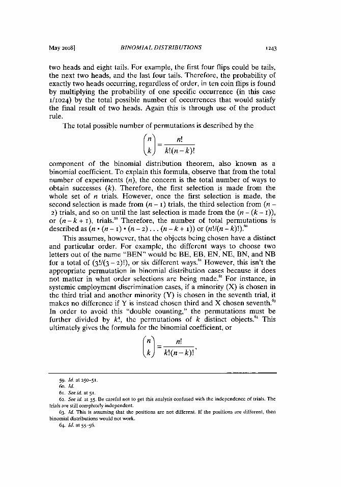
The total possible number of permutations is described by the

n n!

k) k! (n -k)!

component of the binomial distribution theorem, also known as abinomial coefficient. To explain this formula, observe that from the totalnumber of experiments (n), the concern is the total number of ways toobtain successes (k). Therefore, the first selection is made from thewhole set of n trials. However, once the first selection is made, thesecond selection is made from (n - i) trials, the third selection from (n -2) trials, and so on until the last selection is made from the (n - (k - I)),

or (n - k + I), trials." Therefore, the number of total permutations isdescribed as (no (n - I) ° (n - 2) ... (n - k + i)) or (n!/(n - k)!). 6

This assumes, however, that the objects being chosen have a distinctand particular order. For example, the different ways to choose twoletters out of the name "BEN" would be BE, EB, EN, NE, BN, and NBfor a total of (3!/(3 - 2)!), or six different ways. 6' However, this isn't theappropriate permutation in binomial distribution cases because it doesnot matter in what order selections are being made.62 For instance, insystemic employment discrimination cases, if a minority (X) is chosen inthe third trial and another minority (Y) is chosen in the seventh trial, itmakes no difference if Y is instead chosen third and X chosen seventh. 3

In order to avoid this "double counting," the permutations must befurther divided by k!, the permutations of k distinct objects.6, Thisultimately gives the formula for the binomial coefficient, or

k k! (n - k)!'

59. Id. at 250-51.6o. Id.61. See id. at 5I.62. See id. at 55. Be careful not to get this analysis confused with the independence of trials. The

trials are still completely independent.63. Id. This is assuming that the positions are not different. If the positions are different, then

binomial distributions would not work.64. Id. at 55-56.

May 2008]

HASTINGS LAW JOURNAL [Vol. 59:1235

which illustrates the number of ways in which k successes can be selectedfrom a set of n independent trials.6' Therefore, in the BEN example, theonly permutations are BE, BN, and EN for a total of three differentways, which is verified by the formula (3!/(2! ° (3 - 2)!)). Likewise, in thecoin example above, the total number of ways to obtain two heads from aset of ten independent trials is (IO!/(2! • 8!)) or forty-five different ways,which can also be ascertained by simply listing all of the possibilities.66

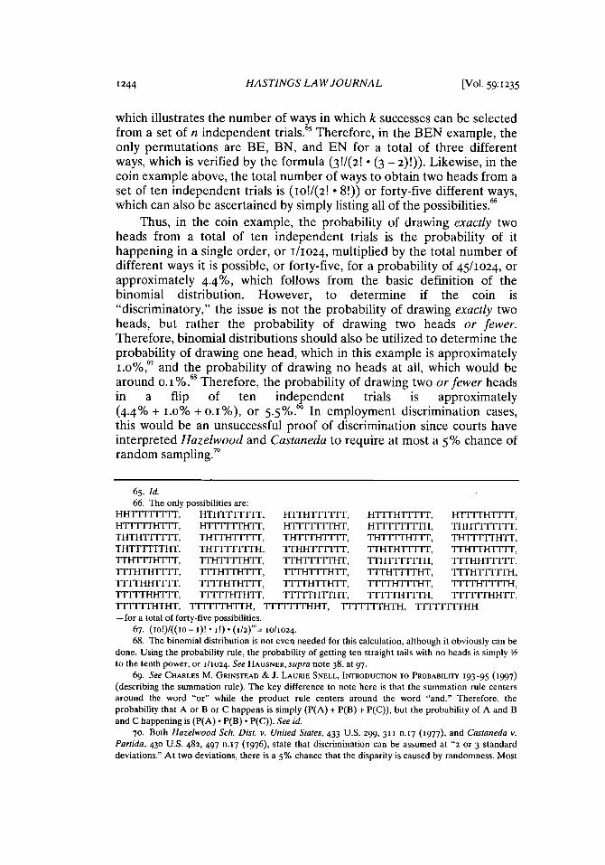
Thus, in the coin example, the probability of drawing exactly twoheads from a total of ten independent trials is the probability of ithappening in a single order, or 1/1024, multiplied by the total number ofdifferent ways it is possible, or forty-five, for a probability of 45/1024, orapproximately 4.4%, which follows from the basic definition of thebinomial distribution. However, to determine if the coin is"discriminatory," the issue is not the probability of drawing exactly twoheads, but rather the probability of drawing two heads or fewer.Therefore, binomial distributions should also be utilized to determine theprobability of drawing one head, which in this example is approximatelyi.o%, 67 and the probability of drawing no heads at all, which would bearound 0.1%.68 Therefore, the probability of drawing two or fewer headsin a flip of ten inde endent trials is approximately(4.4% + 1.o% + 0.I%), or 5.5%. T In employment discrimination cases,this would be an unsuccessful proof of discrimination since courts haveinterpreted Hazelwood and Castaneda to require at most a 5 % chance ofrandom sampling.7"

65. Id.66. The only possibilities are:

HH-TrIII, HTHTITITI, HTrH'TITT=, HTI-rHT=T , I-TTHTIT,HTITTHTI, HTTITrHTT, HI1-111 1 H, HTIMTTH, THHITITI-1,THTHTTT, THTTHT=ITr, TH ITHTI, THTTTHTTr, THTITTHTT,THTTTHT, THTTIHTITH, TTHHTTT, TrHTHTITr, TrHTTHTTT,TTH'IT-HTT, TrHTnTHTr, TTHTT1TTHT, TTHITH ITrH, TTTHHTITVF,TITHTHTIT, THT HTIT, =TTHTITHTr, TTTHT-HT, TTTHTITIH,ITrHHTIT, TTTHTHTTT, TITTHTHTr, TTTHTHT, TTTTHTITH,

TTIT HHTT, TITrHTHTT, TTTHTrHT, TlTITHTITH, TITI1THHTT,TTITTrHTHT, 'ITTITrHTH, TITTrrITHHT, TFITT HTH, TITITItHH-for a total of forty-five possibilities.

67. (1O!)/((1O - I)! " I!) (I/2)"'= 10/1024.

68. The binomial distribution is not even needed for this calculation, although it obviously can bedone. Using the probability rule, the probability of getting ten straight tails with no heads is simply 1 2to the tenth power, or 1/1024. See HAUSNER, supra note 38, at 97.

69. See CHARLES M. GRINSTEAD & J. LAURIE SNELL, INTRODUCTION TO PROBABILITY 193-95 (997)

(describing the summation rule). The key difference to note here is that the summation rule centersaround the word "or" while the product rule centers around the word "and." Therefore, theprobability that A or B or C happens is simply (P(A) + P(B) + P(C)), but the probability of A and Band C happening is (P(A) • P(B) • P(C)). See id.

70. Both Hazelwood Sch. Dist. v. United States, 433 U.S. 299, 311 n.I7 (1977), and Castaneda v.Partida, 430 U.S. 482, 497 n.17 (1976), state that discrimination can be assumed at "2 or 3 standarddeviations." At two deviations, there is a 5% chance that the disparity is caused by randomness. Most

BINOMIAL DISTRIBUTIONS

A problem arises, however, when the number of "successes" is fairlylarge because the binomial computations become exceedingly tedious.7'For example, in Castaneda, since there were 339 jury members that wereMexican-American, it would have been somewhat difficult and timeconsuming7" to use binomial distributions to exactly calculate theprobability that 339 members were chosen, that 338 members werechosen, that 337 members were chosen, and so on.73 Therefore,Castaneda implicitly used a "normal distribution" as an approximation ofthe binomial distribution.74 According to the "central limit theorem,"normal distributions and their bell curves are an extremely accurateapproximation of the binomial distribution as long as the number oftrials (n) multiplied by the probability of a success (p) 75 is equal to at leastfive. 76 It is important to note that while Hazelwood implicitly endorsesthe usage of these approximations, the number of trials and theprobability of a minority hiring in that particular case do not justify usingnormal distributions as an approximation.77 Similarly, many courtsfollowing Hazelwood have inappropriately used these approximationswhen the number of hiring decisions and/or the probability of a minoritybeing hired were not high enough.7s

Nevertheless, if it is appropriate to use normal distributions asapproximations of binomial distributions, then the "standard deviation"of the normal distribution is used to determine the probability that a

courts have followed this 5% rule. See, e.g., HAGGARD, supra note 3, at 84.71. Sugrue & Fairley, supra note 22, at 931; see also ROBERT L. WINKLER & WILLIAM L. HAYS,

STAnISTICS: PROBABILITY, INFERENCE, AND DECISION 226 (1975).72. Though, in this Author's view, not at all impossible. In fact, a computer program could be

written to solve this problem with relative ease.

73. Sugrue & Fairley, supra note 22, at 931; see also WINKLER & HAYS, supra note 71.74. Sugrue & Fairley, supra note 22, at 931-32; see also SAMUEL ESTREICHER & MICHAEL C.

HARPER, CASES AND MATERIALS ON EMPLOYMENT DISCRIMINATION LAW 68 (2OO4). An entire discussion

about normal distributions and why they are an accurate approximation of binomial distribution is

beyond the scope of this Note. For more information about normal distributions, see HAUSNER, supranote 38, at 244.

75. Or the probability of a failure, given by (I -p), but in employment discrimination cases, p will

usually be smaller than (i -p) anyway.76. This number five is not actually part of the central limit theorem, but has been accepted by

most mathematicians as an appropriate value. See HAUSNER, supra note 38, at 244.77. The percentage of the minorities in the labor market was either 15.4% or 5.7%. See

Hazelwood Sch. Dist. v. United States, 433 U.S. 299, 310-1I (977). However, either of these valuesmultiplied by the number of employees hired, or fifteen, is far less than five. See id. In' this Author's

view, it is difficult to understand why Hazelwood did not simply use the binomial distribution, which

did not have overly burdensome computations.78. Sugrue & Fairley, supra note 22, at 926-27; see also, e.g., Wilkins v. Univ. of Houston, 654

F.2d 388 (5th Cir. i98I); EEOC v. Am. Nat'l Bank, 652 F.2d 1176 (4th Cir. I981); Hameed v. Int'l

Ass'n of Bridge, Structural & Iron Workers Local 396, 637 F.2d 506 (8th Cir. i98o); Bd. of Educ. v.

Califano, 584 F.2d 576 (2d Cir. 1978); Otero v. Mesa County Valley Sch. Dist., 568 F.2d 1312 (Ioth Cir.1977); see also JOHN J. DONOHUE III, FOUNDATIONS OF EMPLOYMENT DISCRIMINATION LAW 297-98

(2003).

May 2008]

HASTINGS LAW JOURNAL

disparity in numbers is due to randomness.79 The standard deviation of anormal distribution is described as the square root of ((n * p - (I -p)),where n is the total number of people in the drawing pool, p is theprobability of a success, and (I -p) is the probability of a failure."' If thestandard deviation is exactly one, then there is about a 32% chance thatthe selections were due to randomness; if the value is two, then theprobability is 5 % that it is due to randomness; and if the value is three,then the probability of randomness is 0.3%."

III. THE ERRONEOUS ASSUMPTION OF INDEPENDENT TRIALS MADE BY

BINOMIAL DISTRIBUTIONS

As stated above, the binomial test relies on the "product rule.""B2 Theproduct rule states that the probability of each of the events isindependent of each other event"3 and the probability of a "success" isstrictly based upon the population of the "successes" in relation to thetotal population set.84 This implies that courts using binomialdistributions make a critical assumption based on random sampling inthat every new hiring decision made by the emp loyer is random andindependent of every previous hiring decision. Unfortunately, thisassumption is seriously flawed because "random sampling, which givesrise to the applicability of the product rule, is rarely present in nature orhuman affairs. '

79. ROBERT BELTON ET AL., EMPLOYMENT DISCRIMINATION: CASES AND MATERIALS ON EQUALITY IN

THE WORKPLACE 227 (2004) ("Generally, the fewer the number of standard deviations that separate anobserved from a predicted result, the more likely it is that the observed disparity is not really a'disparity' at all, but rather a random or chance fluctuation. Conversely, the greater the number ofstandard deviations, the less likely it is that chance is the cause of any difference between the expectedand observed results."); see also ESTREICHER & HARPER, supra note 74, at 68-69; HAGGARD, supra note3, at 85; HAUSNER, supra note 38, at 210-12; PAETZOLD & WILLBORN, supra note 6, at 34; Meier et al.,supra note 47, at 145.

80. ESTREICHER & HARPER, supra note 74, at 68-69; HAGGARD, supra note 3, at 85; HAUSNER, supranote 38, at 210-12; PAETZOLD & WILLBORN, supra note 6, at 34; Meier et al., supra note 47, at 144.

8I. HAUSNER, supra note 38, at 210-12; PAETZOLD & WILLBORN, supra note 6, at 34-35; see alsoESTREICHER & HARPER, supra note 74, at 68-69. As described infra, the Court in Casteneda would findan inference of discrimination somewhere between two and three standard deviations. However, asillustrated, there is a significant difference between two and three standard deviations, which begs thequestion of which value is appropriate. See generally Kaye, supra note 48.

82. See HAU1SNER, supra note 38, at 97.83. Normal distributions also require that the trials be independent. HAUSNER, supra note 38, at

244.

84. Recall that in the binomial distribution formula above, the total population set is illustratedby "n," and since there can only be two outcomes in binomial distribution analysis, the number of"failures" is (n - k).

85. See HAUSNER, supra note 38, at 249-50; see also PAETZOLD & WILLBORN, supra note 6, at 32-33; Meier et al., supra note 47, i48-5o.

86. Meier et al., supra note 47, at 153 (emphasis omitted).

1Vol. 59:1x235

BINOMIAL DISTRIBUTIONS

A. HYPERGEOMETRIC DISTRIBUTIONS HELP SOLVE SOME INDEPENDENCE

PROBLEMS

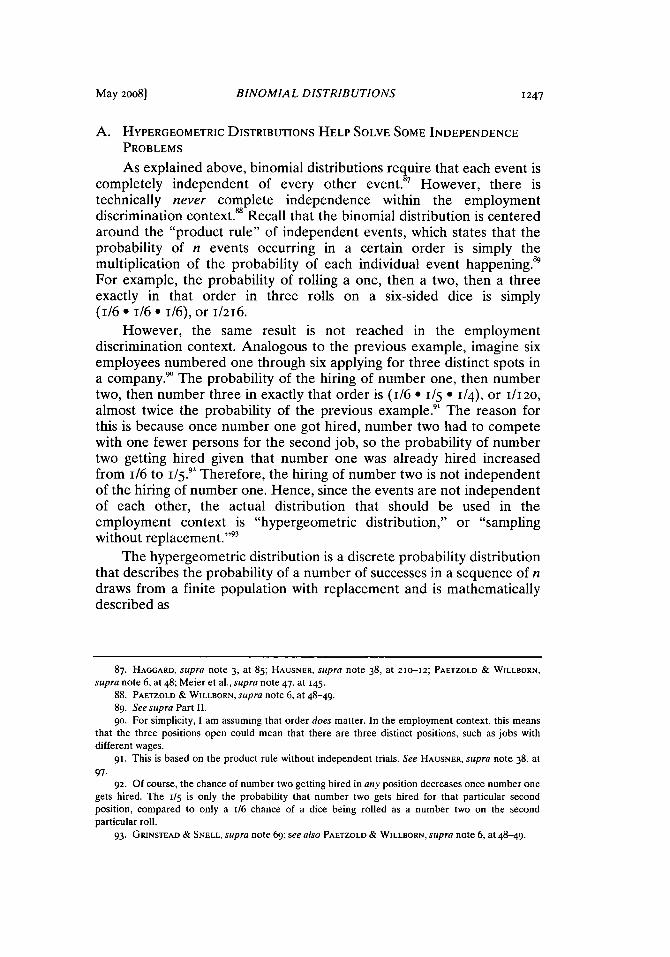
As explained above, binomial distributions reuire that each event iscompletely independent of every other event. ' However, there istechnically never complete independence within the employmentdiscrimination context.8 Recall that the binomial distribution is centeredaround the "product rule" of independent events, which states that theprobability of n events occurring in a certain order is simply themultiplication of the probability of each individual event happening.89

For example, the probability of rolling a one, then a two, then a threeexactly in that order in three rolls on a six-sided dice is simply(I/6 * i/6 * I/6), or 1/216.

However, the same result is not reached in the employmentdiscrimination context. Analogous to the previous example, imagine sixemployees numbered one through six applying for three distinct spots ina company.' The probability of the hiring of number one, then numbertwo, then number three in exactly that order is (i1/6 * 1/5 - 1/4), or 1/120,

almost twice the probability of the previous example.9 The reason forthis is because once number one got hired, number two had to competewith one fewer persons for the second job, so the probability of numbertwo getting hired given that number one was already hired increasedfrom I/6 to 1/5.92 Therefore, the hiring of number two is not independentof the hiring of number one. Hence, since the events are not independentof each other, the actual distribution that should be used in theemployment context is "hypergeometric distribution," or "samplingwithout replacement.

93

The hypergeometric distribution is a discrete probability distributionthat describes the probability of a number of successes in a sequence of ndraws from a finite population with replacement and is mathematicallydescribed as

87. HAGGARD, supra note 3, at 85; HAUSNER, supra note 38, at 210-12; PAETZOLD & WILLBORN,

supra note 6, at 48; Meier et al., supra note 47, at 145.88. PAETZOLD & WILLBORN, supra note 6, at 48-49.

89. See supra Part II.90. For simplicity, I am assuming that order does matter. In the employment context, this means

that the three positions open could mean that there are three distinct positions, such as jobs withdifferent wages.

91. This is based on the product rule without independent trials. See HAUSNER, supra note 38, at97.

92. Of course, the chance of number two getting hired in any position decreases once number onegets hired. The 1/5 is only the probability that number two gets hired for that particular secondposition, compared to only a /6 chance of a dice being rolled as a number two on the secondparticular roll.

93. GRINSTEAD & SNELL, supra note 69; see also PAETZOLD & WILLBORN, supra note 6, at 48-49.

May 2008]

HASTINGS LAW JOURNAL

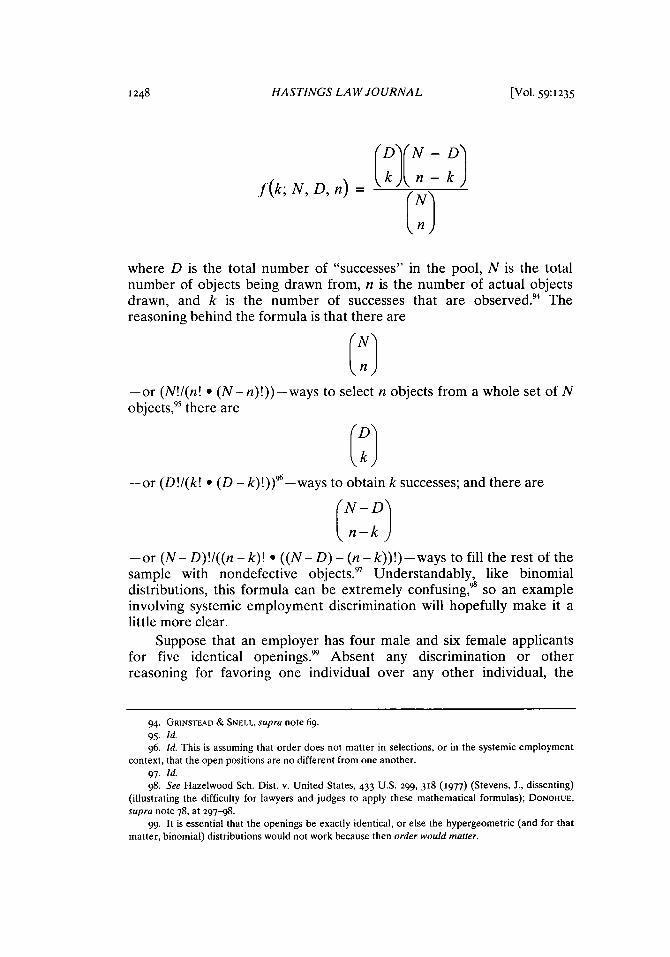
f(k; N, D n) = (N:nwhere D is the total number of "successes" in the pool, N is the totalnumber of objects being drawn from, n is the number of actual objectsdrawn, and k is the number of successes that are observed.' Thereasoning behind the formula is that there are

-or (N!I(n! * (N - n)!))-ways to select n objects from a whole set of Nobjects,' there are

-or (D!I(k! e (D - k)!))6-ways to obtain k successes; and there are

-or (N- D)!I((n - k) ((N- D) - (n - k))!)-ways to fill the rest of thesample with nondefective objects.7 Understandably, like binomialdistributions, this formula can be extremely confusing,0 so an exampleinvolving systemic employment discrimination will hopefully make it alittle more clear.

Suppose that an employer has four male and six female applicantsfor five identical openings.' Absent any discrimination or otherreasoning for favoring one individual over any other individual, the

94. GRINSTEAD & SNELL, supra note 69.95. Id.96. Id. This is assuming that order does not matter in selections, or in the systemic employment

context, that the open positions are no different from one another.97. Id.98. See Hazelwood Sch. Dist. v. United States, 433 U.S. 299, 318 (1977) (Stevens, J., dissenting)

(illustrating the difficulty for lawyers and judges to apply these mathematical formulas); DONOHUE,supra note 78, at 297-98.

99. It is essential that the openings be exactly identical, or else the hypergeometric (and for thatmatter, binomial) distributions would not work because then order would matter.

[Vol. 59:1235

BINOMIAL DISTRIBUTIONS

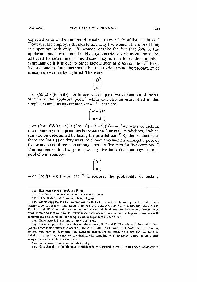
expected value of the number of female hirings is 6o% of five, or three."However, the employer decides to hire only two women, therefore fillingthe openings with only 40% women, despite the fact that 6o% of theapplicant pool was female. Hypergeometric distributions must beanalyzed to determine if this discrepancy is due to random numbersamplings or if it is due to other factors such as discrimination."' First,hypergeometric functions should be used to determine the probability ofexactly two women being hired. There are

-or (6!/(2! e (6 - 2)!))-or fifteen ways to pick two women out of the sixwomen in the applicant pool,'2 which can also be established in thissimple example using common sense.'03 There are

n-k

-or ((io - 6)!/(( 5 - 2)! * ((io -6) - (5 - 2))!))-or four ways of pickingthe remaining three positions between the four male candidates, 4 whichcan also be determined by listing the possibilities. 5 By the product rule,there are (15 * 4) or sixty ways, to choose two women amongst a pool offive women and three men among a pool of five men for five openings.'I

The number of total ways to pick any five individuals amongst a totalpool of ten is simply

-or (IO!/(5! * 5!))-or 252.'" Therefore, the probability of picking

oo. HAUSNER, supra note 38, at 168-70.Ioi. See PAETZOLD & WILLBORN, supra note 6, at 48-49.102. GRINSTEAD & SNELL, supra note 69, at 93-96.103. Let us suppose the five women are A, B, C, D, E, and F. The only possible combinations

(where order is not taken into account) are AB, AC, AD, AE, AF, BC, BD, BE, BF, CD, CE, CF,DE, DF, and EF. Note that this counting method can only be done since the numbers chosen are sosmall. Note also that we have to individualize each woman since we are dealing with sampling withreplacement, and therefore each sample is not independent of each other.

104. GRINSTEAD & SNELL, supra note 69, at 93-96.105. Let us suppose the four male candidates are A, B, C, and D. The only possible combinations

(where order is not taken into account) are ABC, ABD, ACD, and BCD. Note that this countingmethod can only be done since the numbers chosen are so small. Note also that we have toindividualize each male since we are dealing with sampling with replacement, and therefore eachsample is not independent of each other.

io6. GRINSTEAD & SNELL, supra note 69, at 31.io7. Note that this is the binomial coefficient fully described in Part II of this Note. As described

May 2008]

HASTINGS LAW JOURNAL

exactly two women for this particular position would be 60/252

(approximately 23.8%).However, this percentage understates the probability in the

discrimination context because the appropriate question is not theprobability of hiring exactly two women, but rather the probability thatthe employer will employ two or fewer women."" Therefore,hypergeometric functions must also be applied to the probability that theemployer hires only one woman, in this case approximately 2.4%,'" andthe probability that the employer hires no women at all, which is o%. "'Thus, the probability of an employer hiring two or fewer women in ourexample is (23.8% + 2.4% + 0o%),"l or approximately 26.2%. Althoughthis implies that the discrepancy between the employer's percentage ofwomen employees and the percentage of women in the applicant poolhas a decent probability of being due to chance,"2 a different outcome isconceivable when erroneously using binomial distributions, as advocatedby Castaneda"3 and Hazelwood."4

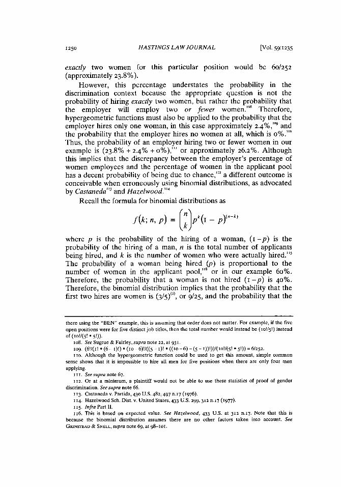
Recall the formula for binomial distributions as

f (k; , p) = nfl~pk(l - P)(n-k)

where p is the probability of the hiring of a woman, (I -p) is theprobability of the hiring of a man, n is the total number of applicantsbeing hired, and k is the number of women who were actually hired."'

The probability of a woman being hired (p) is proportional to thenumber of women in the applicant pool,"6 or in our example 6o%.Therefore, the probability that a woman is not hired (I -p) is 40%.Therefore, the binomial distribution implies that the probability that thefirst two hires are women is (3/5)(), or 9/25, and the probability that the

there using the "BEN" example, this is assuming that order does not matter. For example, if the fiveopen positions were for five distinct job titles, then the total number would instead be (Io!/5!) insteadof (1O!/(5! - 5!)).

io8. See Sugrue & Fairley, supra note 22, at 931.to9. (6!/(1! * (6- i)!) * (io- 6)!/((5 - 0! - ((so- 6) - (5 - 1))!))/(IO!/(5! - 5!)) = 6/252.Iio. Although the hypergeometric function could be used to get this amount, simple common

sense shows that it is impossible to hire all men for five positions when there are only four menapplying.

i i i. See supra note 67.112. Or at a minimum, a plaintiff would not be able to use these statistics of proof of gender

discrimination. See supra note 66.113. Castaneda v. Partida, 430 U.S. 482, 497 n.17 (I976).114. Hazelwood Sch. Dist. v. United States, 433 U.S. 299,312 n.17 (I977).i15. Infra Part II.

116. This is based on expected value. See Hazelwood, 433 U.S. at 312 n.17. Note that this isbecause the binomial distribution assumes there are no other factors taken into account. SeeGRINSTEAD & SNELL, supra note 69, at 98-ioi.

[Vol. 59:1x235

BINOMIAL DISTRIBUTIONS

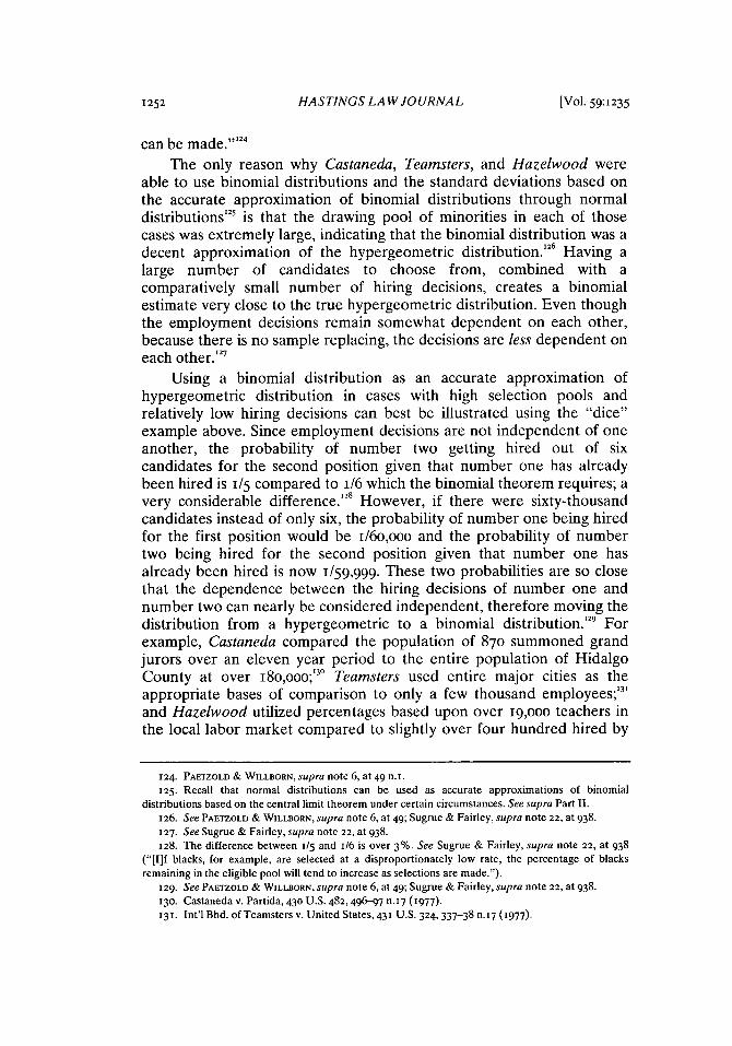
last three hires are men is (2/5)( 3), or 8/125."' Once again following theproduct rule, the binomial theorem therefore provides that theprobability of women for the first two hires and men for the last threehires is (9/25 0 8/125), or approximately 2.3%. However, the hiring doesnot have to occur in this particular order, and there are

(n)= n!

k k! (n - k)!

-or (5!/(2! 3!) = io)-ways of picking two women and three men froman applicant Fool of ten, which can also be shown by simply listing thepossibilities." Therefore, the binomial distribution implies that there is a(io * 2.3%), or approximately 23.0%, chance that the employer hiresexactly two women, which is different from the true 23.8% valuedetermined by hypergeometric functions.

Completing the example, the probabilities of selecting exactly onewoman and exactly no women are also analyzed using the binomialtheorem to find the probability that the employer would hire two orfewer women. The probability that the employer employs only onewoman is approximately 7.7%9 and the probability that the employerhires no women is i.o%.2o Therefore, the binomial theorem produces aresult of (23.0% + 7.7% + 1.o%), or approximately 31.7%. ' Althougheither method yields a result in this particular situation that would drawan inference of no discrimination, the main point is that the differencebetween the two distributions, in this case 31.7% and 26.2%, can lead toextremely significant results where "the binomial model errors on the'conservative' side from a plaintiff's point of view ..... In other words, thiserroneous discrepancy will side against the plaintiff in overstating theprobability of chance.'23 This corresponding understatement ofdiscrimination and overstatement of random chance is why "[i]t is criticalthat the process be modelled [sic] correctly so that appropriate inferences

117. This is incorrect because the sample sets are being erroneously replaced.118. Let's call the women W and the men M. The only possibilities are WWMMM, WMWMM,

wMMwM, wMMMw, MWWMM, MwMWM, MwMMw, MMwwM, MMWMW, and MMMWW.Note that it is not necessary to individualize the men and women since the binomial theorem assumesthat the selection of an individual is independent of the selection of any other individual. SeeHAUSNER, supra note 38, at 252-53.

119. (3/5)" (2/5)'. (5!/(! * 4!)) = 7.68%.12o. Although this can be found using binomial distributions, this can also be found using the

simple product rule of individual trials. GRINSTEAD & SNELL, supra note 69, at 35-37. Therefore, thisamount would be (2/5)' or 1.024%. This should be an obvious error to the reader. It is impossible tohire four men for five positions, however, the binomial theorem lets this be done because it assumesthat every event is independent of the other.

121. See supra note lo7.122. Sugrue & Fairley, supra note 22, at 926-27.123. See id.

May 2008]

HASTINGS LAW JOURNAL

can be made."'' 4

The only reason why Castaneda, Teamsters, and Hazelwood wereable to use binomial distributions and the standard deviations based onthe accurate approximation of binomial distributions through normaldistributions'25 is that the drawing pool of minorities in each of thosecases was extremely large, indicating that the binomial distribution was adecent approximation of the hypergeometric distribution. Having alarge number of candidates to choose from, combined with acomparatively small number of hiring decisions, creates a binomialestimate very close to the true hypergeometric distribution. Even thoughthe employment decisions remain somewhat dependent on each other,because there is no sample replacing, the decisions are less dependent oneach other.'27

Using a binomial distribution as an accurate approximation ofhypergeometric distribution in cases with high selection pools andrelatively low hiring decisions can best be illustrated using the "dice"example above. Since employment decisions are not independent of oneanother, the probability of number two getting hired out of sixcandidates for the second position given that number one has alreadybeen hired is 1/5 compared to i/6 which the binomial theorem requires; avery considerable difference., 8 However, if there were sixty-thousandcandidates instead of only six, the probability of number one being hiredfor the first position would be I/6o,ooo and the probability of numbertwo being hired for the second position given that number one hasalready been hired is now 1/59,999. These two probabilities are so closethat the dependence between the hiring decisions of number one andnumber two can nearly be considered independent, therefore moving thedistribution from a hypergeometric to a binomial distribution.'2 9 Forexample, Castaneda compared the population of 870 summoned grandjurors over an eleven year period to the entire population of HidalgoCounty at over I8o,ooo; ° Teamsters used entire major cities as theappropriate bases of comparison to only a few thousand employees;' 3'and Hazelwood utilized percentages based upon over i9,ooo teachers inthe local labor market compared to slightly over four hundred hired by

124. PAETZOLD & WILLBORN, supra note 6, at 49 n.I.

125. Recall that normal distributions can be used as accurate approximations of binomialdistributions based on the central limit theorem under certain circumstances. See supra Part II.

126. See PAETZOLD & WILLBORN, supra note 6, at 49; Sugrue & Fairley, supra note 22, at 938.127. See Sugrue & Fairley, supra note 22, at 938.128. The difference between 1/5 and 1/6 is over 3%. See Sugrue & Fairley, supra note 22, at 938

("[I]f blacks, for example, are selected at a disproportionately low rate, the percentage of blacksremaining in the eligible pool will tend to increase as selections are made.").

129. See PAETZOLD & WILLBORN, supra note 6, at 49; Sugrue & Fairley, supra note 22, at 938.130. Castaneda v. Partida, 430 U.S. 482,496-97 n.17 (1977).131. Int'l Bhd. of Teamsters v. United States, 431 U.S. 324, 337-38 n.17 0977).

[Vol. 59: 1235

BINOMIAL DISTRIBUTIONS

that particular employer.'3 2

None of these cases illustrates the important fact that binomialdistributions, and the approximations through normal distributions andthe resulting standard deviations, could greatly differ from the accuratehypergeometric distributions.'33 Unfortunately, many lower courts haveblindly followed the formulas put forth in these cases without trulyanalyzing whether they actually fit.'" The damage caused by this in juryselection cases such as Casteneda is not as significant because most juryselection pools are large. The reasons they are so large are that mostadults are eligible for jury selection, the distances between the courthouses and residences are not as significant, and the number of peoplechosen to be on a jury is relatively small.'35 On the other hand, choosingto use binomial analysis instead of hypergeometric statistics in systemicemployment discrimination cases where the number of hiring decisions isa substantial percentage of the eligible pool could produce disastrousresults. This, in turn, could "overstate the likelihood that differences inselection rates could be attributed to chance and understate the statisticalsignificance of the racial disparities observed."'' 6 Therefore, usingbinomial distributions inappropriately as approximations forhypergeometric distributions would cause an understatement ofdiscrimination, making these figures extremely unreliable.'37

B. THERE ARE OTHER INDEPENDENCE PROBLEMS THAT ARISE REGARDLESS

OF WHETHER BINOMIAL OR HYPERGEOMETRIC DISTRIBUTIONS ARE USED

Unfortunately, hypergeometric distributions do not solve allproblems stemming from a lack of independence. Unlike instances ofjury selection, another common reason why each employment decision isnot random is that "[n]o employer truly hires at random from a proxypool."'' 3 The two most common "pooling" problems are "grouping"problems and differences in preference between classes.

i. Grouping Effects Lead to Nonindependent EmploymentDecisions

There are numerous "grouping" scenarios where the group that theemployer selects from is not completely random, such as when "a person

132. Hazelwood Sch. Dist. v. United States, 433 U.S. 299, 303 (1977). The Court in Hazelwood alsorejected the Eighth Circuit's argument that the entire workforce of over one thousand for theemployers should be used for unrelated reasons. Id. at 3 to-i1.

133. See PAETZOLD & WILLBORN, supra note 6, at 46-49; Sugrue & Fairley, supra note 22, at 938.134. See sources cited supra note 19.135. See Sugrue & Fairley, supra note 22, at 938.136. Id.; see also PLAYER, supra note io, at 352 ("A major factor influencing the probative value of

a statistical analysis is the size of the statistical sample. Generally, the smaller the sample size the lessreliable the inference of discrimination.").

137. PAETZOLD & WILLBORN, supra note 6, at 49; Sugrue & Fairley, supra note 22. at 938.138. PAETZOLD & WILLBORN, supra note 6, at 50.

May 2008]

HASTINGS LAW JOURNAL

recruited... recommend[s] or otherwise bring[s] along friends into thecompany [or] success with applicants from a given school or otherorganization may set up a short-term 'pipeline' of future applicants."'39

These grouping scenarios "might be entirely compatible withnondiscriminatory hiring" and is oftentimes the "rule in real worldhiring, not the exception.""'4 This grouping effect makes the nextemployment decision likely to be skewed from the expected value of thedisadvantaged group. 4'

A good illustration of the grouping effect can be shown in anextreme case, EEOC v. Consolidated Service Systems.'42 In ConsolidatedService Systems, the employer of about one hundred cleaners had an8i% workforce consisting of Korean-Americans, despite the fact thatKorean-Americans only made up i% of the general population and 3%of the workforce engaged in this type of business in the metropolitanarea where the service operated.'43 The statistical analysis methodsadvocated by Teamsters and Hazelwood would definitely lead to aninference of discrimination.'" Fortunately, the Court recognized thatthere was not independence in the hiring decisions since the employer'shiring offices were in a heavily Korean-American populatedneighborhood and that most of the applicants came through word-of-mouth recruiting. ' Therefore, when one Korean-American was hired, itwas more likely that another Korean-American would be hired in thenext application decision due to this reference-style recruiting.' 46

In Consolidated Service Systems, the case was such an extremeexample of grouping that the court was able to recognize thenondiscriminatory reason for the disparity in the statistics. However,some form of grouping almost always occurs in employment decisions,and it usually is not detected.'47 The lack of independence between hiringdecisions due to grouping can skew statistics toward either the plaintiffor the defendant.8 Unfortunately, many courts do not recognize thesignificant effects that grouping can have on statistics. Furthermore,

139. Meier et al., supra note 47, at 154; see also ESTREICHER & HARPER, supra note 74, at 78.140. Meier et al., supra note 47, at 154.141. Id.; see also PAETZOLD & WILLBORN, supra note 6, at 49-50.142. 989 F.2d 233 (7 th Cir. 1993); see also ESTREICHER & HARPER, supra note 74, at 78.143. Consolidated Serv. Sys., 989 F.2d at 234-35.144. Unfortunately, the opinion in Consolidated Service Systems does not state exactly how many

employees there were, only the percentages. Therefore, an exact binomial distribution or standarddeviation cannot be obtained. However, based on the percentages, it is extremely likely that the

binomial distributions or standard deviations would have shown that the chance that these hiringdecisions were due to chance would be less than 5%. Id.; see also GRINSTEAD & SNELL, supra note 69,

at 97-99 (describing how to calculate binomial probabilities).145. Consolidated Serv. Sys., 989 F.2d at 236-38.146. Id.; see also Meier et al., supra note 47, at 143.

147. See Meier et al., supra note 47, at 143.148. Id.

[Vol. 59:1235

BINOMIAL DISTRIBUTIONS

these grouping problems would arise regardless of whether binomial orhypergeometric distributions are used.

2. Protected Class PreferenceMany times statistically significant disparities in race or sex are

explained by disparate interest in a particular field or position ratherthan by actual discrimination.'49 Therefore, the applicant pool is notrepresentative of the percentages of classes in the general population.'50

This problem is especially apparent when the general population is usedas the "pool" instead of just the pool of applicants, such as in Teamsters.The cases that use a comparison of the workforce disparities to thegeneral population many times ignore the simple fact that theunderrepresented classes simply do not have as much of an interest in thejob or location of the employment opportunity. Once again, usinghypergeometric distributions would not help solve this problem ofunderrepresented class preference.

C. MORE WEIGHT SHOULD BE PUT ON NONSTATISTICAL ANALYSIS

Statistical evidence is the primary, and oftentimes exclusive,evidence in systemic employment discrimination cases because it iscommonly viewed as the easiest, most concrete, and most thoroughmethod of proving a prima facie case of discrimination.'5' Similarly,courts have found that individual and isolated evidence of discriminationshould not be used with much weight in establishing an inference ofdiscrimination in systemic treatment cases since "individual acts ofdiscrimination are not enough to meet this standard.' ' .2

I believe the opposite logic should be exercised; instead of statisticalevidence providing the primary support with individual treatment assecondary evidence, specific cases and instances should be used ascentral evidence with statistical evidence only persuasive in showingdiscrimination.' 3 Specific and concrete evidence of discrimination should

149. See EEOC v. Sears, Roebuck, & Co., 839 F.2d 302, 324 (7th Cir. 1988); BELTON, supra note 7,at 229; ZIMMER ET AL., supra note 31, at 279; Kingsley R. Browne, Statistical Proof of Discrimination:Beyond Damned Lies, 68 WASH. L. REV. 477,510-12 (1993).

150. ZIMMER ET AL., supra note 31, at 267 ("General population data can be deceptive. Suppose anemployer's typical pool is 99 percent female or a mining company's complement of miners is 99percent male. Is it appropriate to draw an inference of intent to discriminate in these cases?"); see alsoInt'l Bhd. of Teamsters v. United States, 431 U.S. 324, 399-40o n.20 (i977); DAVID C. BALDUS & JAMES

W.L. COLE, STATISTICAL PROOF OF DISCRIMINATION 4.-.3 (i980); BELTON, supra note 7, at 228; Judith P.Vladeck, Sex Discrimination in Higher Education, 4 WOMEN'S RTs. L. REP. 59,74-75 (978).

I5I. Meier et al., supra note 47, at 139-40: see also, e.g., EEOC v. Chicago Miniature Lamp Works,947 F.2d 292, 302 (7 th Cir. 199i); Hazelwood Sch. Dist. v. United States, 433 U.S. 299, 311 n.17 (0977);Teamsters, 431 U.S. at 335-38; PAETZOLD & WILLBORN, supra note 6.

152. PAETZOLD & WILLBORN, supra note 6.153. There exists the belief that statistical data should hold even less weight in employment

discrimination cases, and should instead act as "merely an adjunct to evidence." Browne, supra note149, at 477-

May 2oo8]

HASTINGS LAW JOURNAL

not be used to "simply bolster the statistics."'' 4 This Note has illustratedthat only a limited amount of faith should be instilled in using statisticsand, therefore, should not be used as a primary tool for provingdiscrimination. However, there must be some way of proving a primafacie case of discrimination, and to do this, more weight should be put onindividual evidence and occurrences. If the employer discriminatedagainst one individual in a disadvantaged minority group, the employerwill likely discriminate against others in the group. In these cases,statistical evidence should only be supportive and persuasive of theindividual evidence.

CONCLUSION

Teamsters and Hazelwood used statistical data from standarddeviations based on binomial distributions to prove an inference ofemployment discrimination in systemic disparate treatment cases. Lowercases have since used these standard deviations to create inferences ofdiscrimination.'55 However, "lawyers and judges are often asked toresolve difficult quantitative issues that lie far from their area ofexpertise," and therefore are not aware of, or improperly ignore,important assumptions made by these statistical methods.' Binomialdistributions assume that each employment decision is independent ofevery other decision. Because employment decisions involve "samplingwithout replacement," these decisions are therefore not independent,and a hypergeometric model instead of binomial distributions should beused. However, even if hypergeometric distributions are used or if thebinomial distribution provides an accurate approximation of thehypergeometric distribution, the employment decisions are still notrandom due to grouping effects or minority preference which skew therandomness of the pool. Therefore, other evidence, such as individualinstances of discrimination, should replace statistical data as the primarysource of evidence in showing discrimination in systemic disparatetreatment cases.

154. ROTHSTEIN & LIEBMAN, supra note 7.155. See sources cited supra note 19.

156. DoNoHuE, supra note 78.

[Vo1. 59:1235