öMmföäflsäafaäsflassflassflas ffffffffffffffffffffffffffffffffffff

Discussion Papers

Whole and its Parts:

Micro Foundations of Macro Behaviour

Yrjö Vartia University of Helsinki and HECER

Discussion Paper No. 257 March 2009

ISSN 1795-0562

HECER – Helsinki Center of Economic Research, P.O. Box 17 (Arkadiankatu 7), FI-00014 University of Helsinki, FINLAND, Tel +358-9-191-28780, Fax +358-9-191-28781, E-mail info-hecer@helsinki.fi, Internet www.hecer.fi

HECER Discussion Paper No. 257

Whole and its Parts: Micro Foundations of Macro Behaviour* Abstract The relationship between the whole and its parts is expressed by Synthesis and Analysis operators. Analysis operator gives all the individual micro outputs in terms of their behavioural functions and inputs. This is a very detailed description of the system. Synthesis operator gives the macro output – here the weighted mean of micro outputs – in terms of the same arguments. Also here the input side is described in all its detail. We show how Analysis and Synthesis operators can be decomposed in different meaningful ways. These provide one view towards the micro foundations of macro behaviour. JEL Classification: B41, C43, C81, C82 Keywords: Aggregation, Micro Foundations, Methodology of Economics. Yrjö Vartia Department of Economics P.O. Box 17 (Arkadiankatu 7) University of Helsinki FI-00014 FINLAND e-mail: yrjo.vartia@helsinki.fi * I thank assistant Jussi Lintunen and university lecturer Olli Ropponen for their comments on the paper.

1

Yrjö Vartia, University of Helsinki, Department of Economics

Whole and its parts: The micro foundations of macro behavior1

1. Introduction The views of parts and the whole, of analysis and synthesis, have divided philosophy and science for two thousand years. Do the parts determine the whole or is the whole more than the sum of its parts? Can analysis and synthesis be integrated also in humanities as they are in natural sciences? Of the general philosophy see e.g. Wilson (1998) and Monod (1971). The schemes of unified science (three m's, both Latin and Greek ones) generally, in economics E and in chemistryC are

m

M

)(

)()(

Em

EME

)()(

)()(

PFMCm

CMC

The actual topic of a research area (its macro level) is on the top, a meaningful micro level at the bottom and denotes mathematical - logical methods in their integration, as illustrated by Vartia (2008a). Quantitative and exact methods of chemistry )(C differ from those of econometrics )(E . The micro )(Cm of chemistry is, of course, also part of particle physics )(PFM . We use chemistry as our example from natural sciences. From Wikipedia: “Chemistry is the science concerned with the composition, structure, and properties of matter, as well as the changes it undergoes during chemical reactions. It is a physical science for studies of various atoms, molecules, crystals and other aggregates of matter whether in isolation or combination, which incorporates the concepts of energy and entropy in relation to the spontaneity of chemical processes. Modern chemistry evolved out of alchemy following the chemical revolution (1773).” As we see the macro and micro aspects of chemistry are strongly interrelated. We continue citing Wikipedia: “Chemistry is the scientific study of interaction of chemical substances that are constituted of atoms or the subatomic particles: protons, electrons and neutrons. Atoms combine to produce molecules or crystals. Chemistry is often called "the central science" because it connects the other natural sciences, such as astronomy, physics, material science, biology, and geology… The periodic table of the chemical elements is a tabular method of displaying the chemical elements. Although precursors to this table exist, its invention is generally credited to Russian chemist Dmitri Mendeleev in 1869. Mendeleev intended the table to illustrate recurring ("periodic") trends in the properties of the elements. The layout

1 An extended version of a paper presented in the 3rd Helsinki- Tartu Symposium in Economics, Helsinki 13-14.5.2005

2

of the table has been refined and extended over time, as new elements have been discovered, and new theoretical models have been developed to explain chemical behaviour. The periodic table is now ubiquitous within the academic discipline of chemistry, providing an extremely useful framework to classify, systematize and compare all the many different forms of chemical behaviour. The table has also found wide application in physics, biology, engineering, and industry. The current standard table contains 117 elements as of 27 January 2008 (elements 1-116 and element 118).” These citations show the close connections between the micro )(Cm and macro

)(CM aspects of chemistry. The periodic table explains the atomic reasons for recurring similarities of different compounds. The special mathematics and physics of integrating the micro and macro chemistry )(C are described in Wikipedia as follows: “Theoretical chemistry is the study of chemistry via fundamental theoretical reasoning (usually within mathematics or physics). In particular the application of quantum mechanics to chemistry is called quantum chemistry. Since the end of the Second World War, the development of computers has allowed a systematic development of computational chemistry, which is the art of developing and applying computer programs for solving chemical problems. Theoretical chemistry has large overlap with (theoretical and experimental) condensed matter physics and molecular physics.”…“Computational chemistry is a branch of chemistry that uses computers to assist in solving chemical problems. It uses the results of theoretical chemistry, incorporated into efficient computer programs, to calculate the structures and properties of molecules and solids. While its results normally complement the information obtained by chemical experiments, it can in some cases predict hitherto unobserved chemical phenomena. It is widely used in the design of new drugs and materials.” We see that the mathematics and more generally the methodology of integration of micro and macro aspects in chemistry are highly specialized and technical subjects. The periodic table and similar simplified theories tell however qualitatively what kind of results can be expected. Lagerspetz (1966, a Finnish professor of zoology) poses the question of reductionism of water molecule. Is it possible to derive properties water (say that its density is highest at +4 degrees of Celcius) from the properties of hydrogen and oxygen? According to him “the whole is more than the sum of its parts” is a relative property of theories. The whole can be “more than its parts” only with respect to some theory; the additivity or non-additivity of the wholes and the emergency of their properties are relative concepts. It makes sense to speak of “the emergency” of properties only if we announce in respect to what theory these properties are emergent (Lagerspetz 1966, p. 42-43). The extraordinary behavior of water density in the temperature interval 0 … 4 requires hard mathematics and apparently quantum theoretical effects to be explained. Also Ketonen (a Finnish professor of philosophy, 1976, pp. 148-155) considers what “whole” and “parts” mean and what means that “the whole is equal to or else than the sum of its parts”. If 11 g of hydrogen gas is burned in 89 g of oxygen we get 100 g of

3

water. In this case we agree that the whole, water, which however in respect to its weight is the sum of its parts, in terms of the properties is else than the sum of its parts hydrogen and oxygen. The whole has essentially different properties than its parts, Ketonen (1976, p. 149). … The concept “sum” or “addition” in these considerations is clear only in mathematics and formal logic. Even there the concept “sum” has different meanings according to what kind of objects we are summing. The sum of natural numbers and positive quantities comes usually to mind when sums are considered. But in mathematics and logic sums of complex numbers, vectors, matrixes and classes are talked about. … “The whole is the sum of its parts” is in all these cases a logical truth, because the sum is so defined that it has this property. Ketonen goes on analyzing cases when this additivity does not hold. If there is no theory according to which the properties of a whole W can be derived from the properties of its parts nPPP ,...,, 21 , we can say, that the whole is different to (or more than) the sum of its parts. Ketonen defends the argument that new and better theories narrow the scope of such strongly emergent or non-additive wholes W. In philosophy parts and the whole appear as analysis and synthesis, see Niiniluoto (1983, 156-165). Latin translations of these Greece terms are resolution and composition. Reductionism is considered in Niiniluoto (1983, 255, 289-296). As a specific example of the level of difficulties modeling and integration of atomic and ordinary macro scales a good example is the density anomaly of water at 4 C , see e.g. “Density of water and ice”, “Dipolar nature of water” and “Water model” from Wikipedia. Integration of the different scales of observation is ordinarily a complicated modeling enterprise and more difficult than describing the facts of these scales separately. However, in natural sciences macro and micro scales are well integrated and the macro phenomena can be reduced to micro phenomena and their interactions. This ends our excursion to natural sciences and chemistry, where micro and macro levels are so strongly mixed that their boundaries have almost disappeared from sight. Economics is not yet at the stage that its micro and macro aspects are so strongly integrated. Now we turn to economics and statistics. The paper is organized as follows. The general motivation reviews the basic concepts and introduces them in terms of descriptive statistics and basic mathematics, especially function theory. Third chapter introduces the Analysis operator, which represents all the relevant micro information. The next chapter is about the Synthesis operator, which maps the micro level information on the macro scale mean of its outputs. Linearity of the Analysis and Synthesis operators makes it possible to decompose Actual Behavior as the sum Common Behavior + Heterogeneity Effects. Furthermore, Common Behavior decomposes to Representative Behavior + Non-linearity Effects. Special emphasis is directed to affine behaviors, where Non-linearity Effects vanish and to parallel behaviors, where Heterogeneity Effects vanish. Chapter 4 discusses approximations of Actual Behavior for small changes of input variables. It is conjectured that normally both Non-linearity and Heterogeneity Effects are frozen and thus practically constant. Thus for small changes and normal conditions changes in Actual Behavior and Representative Behavior are approximately the same even without affine and parallel behaviors. Appendix represents these ideas in a condensed and hopefully more readable form.

4

2. The general motivation Aggregation becomes extremely messy, if explicit functional forms and rather elementary mathematical methods are used. It becomes too abstract and also hard to follow, if more general mathematical methods (such as Function Theory, Functional Equations, Abstract Algebra, Index Number Theory) are applied. Therefore, both elementary and abstract approaches would give rise to difficulties. Aggregation is a difficult subject! We have to follow both routes –elementary parametric functional forms for concreteness as in Vartia (2008b) and general mathematics with some new concepts and techniques for generality. New mathematical concepts, such as the A- and S-operators, are needed to see the forest from the trees. In these operators, more accurate notation to separate functions and their arguments is required to operate with different heterogeneous behaviors and contingent conditions which the agents may have and experience. The former approaches have mostly been either too narrow (specialized) or too wide. Some writers considered the general function theoretic possibilities of aggregation and some other the two related problems of aggregation and estimation at the same time. These are only some of limiting cases of the wider possibilities. The interplay between concrete cases and new mathematical notation and methods is crucial and cannot be avoided. It is unfortunate, that the reader cannot be guided and motivated in every detail –that would make the journey too long. Chipman (1976) considered the aggregation problem using generalized Moore-Penrose inverses in his 220 pages monograph. He refers to more than 25 distinguished mathematicians, statisticians and economists who have tried to make sense in the aggregation problem during roughly 40 years in his 24 pages long reference list. Five of them have got a Nobel Price in Economics so that inputs allocated to these questions are considerable. After 40 years of intensive research on the area, writers gave up and withdrew from it roughly 30 years ago. Evidently, the problem was considered as unsolvable or too difficult to solve. Most of the “solutions” were negative ones: aggregation is normally impossible. It is possible only under conditions, which are usually described as very restrictive. But practical economists went on assuming representative agents and behaviors as if that would have been the outcome and suggestion of the researchers. Their suggestions were exactly the opposite. There must have remained something important undiscovered in the issue. We consider units (parts, agents, atoms, molecules) all reacting to their circumstances in their given way. How can this be formalized? Consider a given partition of a set )()(

1iAiAA n

i

representing both the “the whole” and its “parts”. It divides A into its constituent non-intersecting subsets. Let the outputs (“reactions”) ))(( iAyyi be numerically given variables, either scalars or vectors. Extensive measurement is an important special case. Then the sum

))((...))1(( nAyAyY has a concrete meaning or makes sense. Actually this total

5

makes sense already for quantitative variables measured on interval scale, see Vasama and Vartia (1980). Absolute zero does not exist on interval scale (say in ordinary temperature measurement) unlike for ratio scale variables (length, weight, consumption, etc). In economics, such variables ))(( iAy are often current or fixed price values of )(iA . Similarly, let ))((...))1(( nAxAxX be such a total value and Q

))((...))1(( nAqAq , where ))(( iAq = frequency of some basic units in )(iA . There are several possible choices for these basic units; say persons/households/ apartments/blocks/customer codes for people and atoms/molecules/cells for organisms. We use some convenient units to count frequencies ))(( iAq of parts or agents in )(iA . More generally, we call any frequency valued variables (say number of children for families or protons for molecules) as counters. Some twenty years ago a Finnish economist Eetu Tuomainen wrote columns in the Talouselämä (an Economic Magazine in Finland). He asked once the readers to think what they would take with them to a desert island. Only one wish is granted. A Swish knife? A spade? Nothing of that kind. Eetu Tuomainen would take the mean! Without that nobody could manage in such harsh conditions: how could one decide without it what is the proper way to act, not too much or too little. We require benchmarks for which the possible choices are compared. This is the Golden Mean or Rule of ancient times. Thus consider means of real variables or vectors. All means such as

))((/))((/ iAqiAyQYy QXx /

are expressed as corresponding per capita values in these basic units. Note that

))(())((

))((/))(())((

))((/))(())(())((

))((/))((/

iAxiAw

jAqiAxiAq

jAqiAqiAxiAq

jAqiAxQXx

in self-explanatory notation. Here ))((/))(())(( jAqiAqiAw are normalized frequencies, which sum to unity. All means QXx / can be expressed as either w- or q- weighted means over conditional means ))((/))(())(( iAqiAxiAx . This is the law of iterated means. The same weights apply equally to all quantitative variables. For example, x and y may be income and consumption and let frequencies count households. Then x and y are income and consumption per household, i.e. similar per capita figures.

6

Complete accuracy is not required in these matters as frequencies in terms of different parts or units are normally slowly changing structural variables and more or less proportional to each other. Instead of households one may count consumption units (on some equivalence scale). Then all means per consumption unit would be exactly proportional to previous means per household. The proportionality factor is the ratio of household and consumption unit frequencies (or its inverse). We have xQQQXQQQXx )/()/)(/(/ More generally, weighted means can be shown to be rather insensitive for minor changes in the weighting. Transformations from on choice of unit to another are by no means trivial operations and people not familiar with accounting systems, sampling techniques and ratio estimators in sampling surveys should not jump to hasty conclusions by intuition. Important more difficult applications in weighting occur in regression analysis (weighted regression in case of heteroscedastic errors), in sampling (stratified and cluster sampling) and almost everywhere in index number theory. We have given above a short and intuitive review of most basic things in weighting. It hopefully motivates our choice to consider some partition 2 )()(

1iAiAA n

iof

the basic units (parts, agents or objects) and treat its frequencies ))(( iAq as constants in weighting, at least in preliminary. If all subsets are singletons or sets with one unit only, )()( iaiA , then )(),...,1( naaA and 1))(())(( iaqiAq . This is the ideal case, where all intended units are observed and measured separately and the weighting reduces to uniform or equal weighting niaw /1))(( and ))((/ 1 iaynYy n . Equally weighted mean y is called also an unweighted average, somewhat illogically. Starting from this ideal case, we return to the q-weighted means above, if instead of the atomistic partition to singletons our observations are from some more general partition )(iAA . This situation resembles in many ways the stratified sampling scheme in the case of proportional allocation.

3. The Analysis operator A Consider all functions if mapping any set to output space Y; they form a function space denoted by )( Y . We take the output space Y as some linear space over real scalar multipliers. Scalar multiplication and addition are defined in Y and they obey their ordinary rules3. Then the linear combination Yyy 2211 whenever Yyy 21, and s´ are real numbers. This is sufficient to make also

2 The sigma-notation (instead of the union-notation) shows that we are considering a partition. 3 We apply freely mathematical results from standard textbooks such as Apostol (1963), Lehto (1969, 1971) and Kolmogorov and Fomin (1970).

7

)( Y a linear space of functions. More explicitly, if )(, Ygf are two such functions, then also gf defined by )()())(( xgxfxgf belongs to )( Y . Clearly also )( Yf for any R . Note that no structure is needed for the input space for these results to hold. More concrete special cases of this are functions of )( LR , where KR . Dimensions (K, L) , the number of input and output variables, can be arbitrary. Real functions of real variables

)( RRf defined for all real numbers make the mathematically simplest case.

Exercise 1: Consider the case )( R when Rb,0 and n = 10. Interpret bx ,0 as income and take the 10 agents in )10(),...,1( aaA as families having roughly the same background variables (say married couple, one child of age between 5 and 7 years, both working, living in southern Finland in a town, etc) and

))((())(( iaxfiay i are possible consumption functions for them. They just show how consumption could be related to their income. If you are given 10 actual consumption – income points for them for 2004 (evidently yearly figures), these determine only one point for every family. How should you continue the graphs of the 10 consumption functions to nearby incomes? How do you interpret the 10 curves or functions, if they are to be continued for the whole range of incomes bx ,0 ? Do you take them as choices or possibilities for other years or as alternatives for 2004? Would you like to add or remove some background variables? Do you think that the whole task does not make much sense? What else should be done? Would you like to widen the input space by the background variables and add other families? Why?

Exercise 1 shows that there are several obstacles and questions to get even started. We are not prepared to discuss such basic problems of describing actual things with numbers in this paper concerning aggregation. We just note that the researcher himself should give some sensible meaning for his behavioral functions, say for the consumption functions ))((())(( iaxfiay i above. In opinion, the consumption function should aim at answering what would have happened if matters had been differently. Evidently there are many problems and controversies, because only few seem to have thought these questions seriously – or do see any reasons to do it.

As technical point, we note that our behavioral functions should be continued not only in the surrounding of some observed or imagined points, but for their whole definition set. Functions should be defined for all the points of their definition sets, because otherwise they are not functions. We suppose this being done, in one or another way. How this I done or for what reasons, does not interest us here. We take it for granted that the functions have some sensible role to start with. We are not discussing estimation or other even more general and diffuse modeling problems. General motivations for our setup have been given in our previous paper Vartia (2008b).

We shall investigate in the paper what kind of macro behavior the given micro behaviors produce whatever their inputs happen to be –of course assuming that they have some sensible meaning to start with. The problem of the paper is shortly as follows: What follows from the given micro behaviors. This is intended to be primarily a mathematical study.

8

After the implications of this setup have been cleared, we can restrict the arguments of the functions to smaller changes around some observed points.

To avoid problems of input space averaging, we consider in this introductory paper only the case of singleton subgroups )()( iaiA for some conventional choice of elements or units )(ia , say employees, households, firms, apartments, areas, business premises, elementary aggregates in index calculations etc. We assume that similar type of behavioral functions if make sense for them and take these as known.

Example 1: Typically if )( LR , where KR . For instance, in demand

studies of Finnish households we may have pmfd RRN01,0 . Here d = the maximum number of “dummies” or indicators, f = the maximum number of counters and (m, k) give the maximum number of quantitative unrestricted and non-negative input variables, respectively. Examples of counters are the number of children and cars, which can be either zero or some natural number. They get values in ,...1,00N . Their upper limits are fixed for convenience to remove ridiculous values, say more that 230 children in a household. Inclusion in

pmfd RRN01,0 instead of equality allows that. Thus behaviors may have K = d + f + m + p input variables (several dummies4 and counters in addition to the quantitative inputs) and also vector outputs. Such definition sets are very complicated sets of KR . Indicators and counters get only integer values and that makes the whole Cartesian product (and thus ) a non-convex subset of KR . This means that the mean values of two points in – the straight lines connecting them - do not normally belong to it. This is quite awkward, especially when we want to calculate means of the input vectors over agents. They would normally lie outside of , though all individual inputs lie in it.

The simplest way to remove these problems seems to make the input set convex by extending it to its convex hull. At the same time all agent-functions are extended (by interpolation) to get some reasonable values in the previous “holes” or areas between the actual integer values of the discrete inputs. This means treating the discrete inputs for mathematical convenience as if they were continuous. It is a standard method to treat discrete variables as continuous when they get large values, as e.g. the size of a population in an area. We extend this practice also for small values. Discrete variables can keep on getting their natural integer values only; just their functions are extended to all real values between them.

After such a convexation an awkward pmfd RRN01,0 is turned to a wider definition set Kc R having no more holes in it. All previous functions

if )( LR are interpolated to the widened function space )( Lc R . After

4 Indicators/dummies code qualitative properties by zeros and ones, which are in fact logical truth-values. Here quality changes to quantity in aggregation: the mean values of indicators are relative frequencies (or probabilities) which are quantitative variables. Thus indicators can be considered both as qualitative and quantitative, depending on the point view. Fuzzy Logic and Probability Theory are both based on this, from different angles. Any more comments on them are avoided in this introductory paper.

9

this we can take any means of the inputs x also as inputs5 and calculate values such as )(xfi . We call this treating the discrete inputs as if they were continuous. The idea of this trick is getting the means of the inputs inside the function.

For 700 commodity groups L = 700. Usually we consider output components (say quantities of different commodities bought) one by one, which amounts to setting L = 1. Nothing hinders the number n of households being a realistic number, say several millions. Unless otherwise stated, the functions if are allowed to be arbitrary: for instance, only piecewise continuous, locally affine or nonlinear, such as any piecewise defined locally cubic functions of the quantitative inputs.

Estimation problems6 are not discussed in the paper: we concentrate on the aggregation of the behaviors from micro to macro level. Our approach is that of general mathematics and our main methods are function theory, abstract algebra and functional equations. We allow arbitrary constant weights 0))(())(( iaqiAq . The simplest of them is the equal weighting 1))(( iaq , which would result in

njaqiaqiaw 1))((/))(())(( .The same set of weights is assumed to apply all the

time. Normalized weights ))((/))(())(( jaqiaqiaw sum always to unity. Now consider some )( Yfi ( ni ,...,1 ) as the behavioral functions of the n agents or units )(ia . They define the whole micro system as follows: )))((())(( iaxfiay i “One by one description” where ))(( iax input and ))(( iay output for )(ia in their respective spaces. Inputs

))(( iax may get any values in independently of each other and outputs move in their linear output space Y as determined by if . Addition and scalar multiplication for any functions )(, Ygf are defined as normally by point-wise addition and multiplication: )()())(( xgxfxgf and ))(())(( xfxf . Thus gf and f become functions of )( Y . Similarly functions )( Yfi determine the average behavior f as follows

5 If some x-variable denoted by z is either an indicator or counter, all its actual values are integers starting from zero. We may say that its averaging process changes quality to quantity. Means z may concretely be 0,735 or 73,7 % for an indicator like “having an internet connection” and 1,414 for “number of children”. Such intermediate values would appear as actual observations on semi-macro levels. For convenience of representation, micro behaviors are supposed be defined by interpolation also for such intermediate values. Such values do not appear as micro observations, but they naturally appear for their means. On a more philosophical level most of our concrete observations – say of a table – appear as means and “quantities” although tables are “mostly full of holes” according to atom theory. We have the habit of ignoring these questions in daily life. 6 Actually indicators are often superfluous in the analysis, because they are often agent-constant (say gender) and can in those cases be imbedded in the agent-specific behaviors. On the other hand, marital status and home location really are variables. Indicators are so popular in the estimation that we have included them here. Note that we do not assume that “dummies” have only intercept effects: they can affect behaviors more profoundly, say any “slopes”.

10

ffiawf i

n

i 1))(( or )())(()(

1xfiawxf i

n

i for all x .

This is a crucial definition and the reader should clear it out e.g. in the case of

)( R of the exercise 1. Note that this definition alters the arguments x in no way, so that e.g. all dummy inputs act exactly as before. Only outputs are averaged and that makes sense, when Y is a linear space. As a linear combination of sfi ´ also )( Yf . The average behavior f has an important role both in the macro and micro behaviors. It has an important role, but it is not the only actor in the macro behavior, contrary to what most macro texts in economics try to defend. The researchers of the aggregation problem seem to have concentrated on two polar questions: 1) When the average behavior f really is and 2) why it supposedly is not “in general” or ”in reality” the sole actor in the show. The quarrel could continue indefinitely long, because the participants are putting their approximations in different places and do not want to take into account the arguments of the other side. That could reveal weaknesses in their approach. It could cast too much light on their previous contributions and more generally on their paradigms, see the preface of Fisher (1992). This is a typical way how personal interests hinder scientific progress. It seems to be a good time to break the 30 years silence in economics. Next we separate all different constituents of the micro system and order them agent-wise in their appropriate vectors. Using simplified notation for the inputs ))(( iaxxi and outputs ))(( iayyi , we have fewer brackets and more sub-indices in )( iii xfy . The column vectors are in terms of these

n

n

Y

y

y

y

1

, n

nx

x

x

1

, n

n

Y

f

f

f )(

1

Next write all the micro equations in terms of these vectors and the A-operator:

),(

,

,

)(

)(

)

11111

xfA

xf

xf

A

xf

xf

y

y

y

nnnnn

.

11

The Analysis operator A (shortly A-operator) separates the function symbols from their arguments agent by agent and outputs their “outcomes” iiii xfxf )( , a formal product actually. This product interpretation ii xf is mostly applied in Linear Algebra for linear functions and their arguments. A-operator is both a notational and conceptual trick. It reveals the logical parts of the micro system. In addition to its traditional one by one -description, the micro system can now be expressed very shortly and elegantly: ),( xfAy The Basic Micro View (Eight Symbol Formula) It takes some time to get accustomed to this new notation and to realize its importance. The analysis operator in ),( xfAy is best read backwards. It shows, how the outputs are explained in terms of its constituent parts: all the behaviors f and inputs x. It gives the Analysis of the micro system. Reading forwards from behaviors and inputs to outputs may first make this A-notation look unnecessary, ”as everything has been said already in )( iii xfy ”. No, it is not; we need it. In raises the behaviors to the front and separates them from the inputs. The A-operator is like integration, summation and derivation linear in its functional arguments: For all sequences of behaviors nYgf )(, and all real multipliers R21, ),(),(),( 2121 xgAxfAxgfA . This holds identically for all possible input sequences nx . We leave it for the reader to verify. It is a simple exercise in general algebra and you would not appreciate it, if we wrote it down for you. Note how difficult its discovery would have been without proper notation. Next make an important connection with the macro behavior by writing iii ffffff )( or )()()( xfxfxf ii . This pulls heterogeneous behaviors )(xfi aside and brings average behaviors )(xf to the front. Inserting actual inputs gives )))((()))((()))((())(( iaxfiaxfiaxfiay ii which reads for all agents together ),(),1( xfAxfAy Summary of micro behaviors. This follows immediately from the linearity of A and from the identity fff 1 . Note that )1,...,1(),...,(1 ffff means “ f applied for every unit or agent”.

12

Average behaviors act like benchmarks against which all behaviors are compared. How else could we effectively describe e.g. 2 million different consumption functions, which is a typical case in a small country? Should we tell two million stories without any comparisons? Actually the heterogeneous behaviors mostly cancel each other away at the macro level. But this does not occur “necessarily”, which has caused the controversy mentioned above. We will show after a while when and why. 4. The Synthesis operator S We first mention that the average output was defined in the general motivation as the w-weighted mean n

iiayiawyy

1))(())(( .

Now insert ),( xfAy which is in component form ))((())(( iaxfiay i : n

i i ixfiawxfAy1

))(())((),( In accordance with the A-operator and the chosen weighting scheme, define finally the synthesis operator S by ),(),( xfAxfS . These definitions are completely synchronized: The synthesis operator maps the inputs to the average output: yxfS ),( . The linearity of the A-operator transforms immediately also to the S-operator: For all sequences of behaviors nYgf )(, and all real multipliers R21, ),(),(),( 2121 xgSxfSxgfS . This holds identically for all possible input sequences nx . This is a remarkable fact, though its proof is self-explanatory:

),(),(),(),(

),(),(

),(),(

),(),(

21

21

21

21

2121

xgSxfSxgAxfA

xgAxfA

xgAxfA

xgfAxgfS

The real significance of the Summary of micro behaviors reveals itself on the macro level, where heterogeneous behaviors turn into Heterogeneity Effects HE(x):

13

),(),1(),(),1( xfSxfSxfAxfAy . Shortly ),(),1(),( xfSxfSxfS because fff 1 or )()()( xHExCBxAB . Read: Actual Behavior = Common Behavior + Heterogeneity Effects. Furthermore, Common Behavior can be decomposed as Representative Behavior + Non-linearity Effects as follows: ),1(),1(),1(),1( xfSxfSxfSxfS or )()()( xNLExfxCB These are usually very complicated mathematical functions, which depend on all the micro behaviors and all the circumstances (inputs), where the agents happen to be. But they turn out to be mathematically manageable. Their complexity can be compared to the Gibb´s Ensemble or Fock Space of statistical physics, where the phase space of many particles7 is modeled similarly. We also use similar notation for averages and inner products, the main mathematical tools in the area. But we have allowed and added heterogeneity of behaviors to all that. Note that the Common Behavior is still a complicated function for several reasons, though it looks simple. Its main complexity arises from the fact that the agent-inputs are free variables in some high dimensional space, say pmd RR1,0 : )())((())((),1()(

1xfiaxfiawxfSxCB n

i.

The last expression looks nice, but leads easily to misunderstandings. CB depends on all the behaviors. Formally ),1()( xfSxCB maps all sequences nYf )(

and nx to Y , just like ),()( xfSxAB and ),1()( xffSxHE do. They have both functions and ordinary arguments as their inputs. They can be called functional – functions. Example 1: Simplify the function space )( Y as much as possible into

)( RR . Take all sfi´ as affine functions xiixfi )()()( . Then xxf )( , where aiiaw )())(( and similarly for . These give

7 Say more than 6,022142* 2310 = the number of molecules in one mole of gas. One mole of hydrogen –the definitely most common of all roughly 100 elements in the universe - weights only 1 gram.

14

x

x

iaxiawiaw

iaxiawiaw

iaxiawiaw

iaxiaw

xfxCB

n

i

n

i

n

i

n

i

n

i

n

i

11

11

1

1

))(())(())((

))(())(())((

))(())(())((

))(())((

)()(

The “quick and dirty-method” (which easily leads to absurdities) gives this outcome easily once we know the correct result:

)(

)(

)()(

xfx

xfx

x

xfxCB

For affine heterogeneous behaviors, the common behavior depends on the average/representative behavior (as always) and the mean input only - and nothing else. This is best stated operationally: )()()( xfxfxCB .

This is a strong result, which actually holds also in the function space )( LK RR for all K and L. If its functions if are all affine (and otherwise arbitrary),

then also )( LK RRf is affine and the Common Behavior depends on KRxx only: )()()( xfxfxCB . We suggest, that the reader tries to write

these simple looking formulas using standard matrix notation, first for L = 1 and then for general L. It is not so simple. Before turning to the converse of these theorems, we add some comments. In this direction things are rather clear and “simple”. For instance, it is clear, that affine heterogeneous micro functions always generate affine average behaviors. Can an affine average behavior arise otherwise? Yes, but only occasionally, for some restricted agent-arguments, where their behaviors “looks like affine”. Affine average behavior can arise generally (i.e. for all possible micro arguments) only if all micro behaviors are also affine.

Example 2: Converse results of Example 1. This direction is much more difficult and is based on some rather deep (but well-known) results of Functional Equations, see Aczél (1966). We return to the simplest case )( LK RR , where K = L = 1, which is hard enough. Example 1 shows that for affine micro behaviors

)()(),1(: xfxfxfSRx n ,

15

the common behavior depends on the mean of the inputs Rxx only. Also the

converse result holds: If the functional equation )()(: xfxfRx n holds, then the function f must be affine. For n = 2 this functional equation reads

)2

(2

)()( 2121 xxfxfxf .

Affine functions are the only minimally regular solutions of this functional equation.

By the way, in this affine case the Heterogeneous Effect ),cov(,)(),()( xxxfxfSxHE . It has many other equivalent

representations:

xxxxx ,,),cov(),cov(),cov( .

The deviation operator can be moved around completely freely in the statistical covariance-expressions but must appear at least once in the general inner product-expression. 0),cov(,)( xxxHE iff all agent-slopes are equal. This leaves all intercepts totally free, which means that intercept heterogeneity has no macro effects for parallel affine micro equations: xixfi )()( . This deals with affine functions only, but generalizes heavily.

Actually completely generally: If if are parallel shifts from each other, called a parallel family, then )(xHE vanishes identically. More surprisingly, also the converse is valid: If )(xHE vanishes identically, then sfi ' form a parallel family. We have

)()()( xgixfi , where both the shifts and the g-function can be arbitrary. The macro behavior does not change at all if all the micro behaviors are replaced by the same average behavior )()( xgxf . Symbolically: If sfi ' form some parallel family, then ),1(),( xfSxfS , and conversely. This very strong result holds in any function space )( Y , where Y is a linear space.

Aczél (1966) considered carefully the Functional Equation when )(, RRgf

)2

(2

)()( yxgyfxf The Jensen Equation.

If both f and g are differentiable, then taking partial derivatives from both sides gives 2

121

21 ))(()( yxgxf xx or ))(()( 2

1 yxgxf xx . The left side depends on x only, as the right hand side depends also on y. This is impossible unless both derivatives “depend on nothing” or are constants. This implies that both f and g must be affine and actually the same: xxgxf )()( . This clearly solves the equation. But in this solution of Jensen Equation we applied the differentiability assumption. Aczél shows that the same solution arises with minimal regularity for f and g, say continuity in just one point or if they are bounded in any short interval. But

16

without any such regularity, also irregular and really wild Hamel-solutions arise (in addition to the extremely regular affine ones).

This generalizes: The only minimally regular solutions of

)()( xgxf , Generalized Jensen Equation GJE

where )()( iyiwy = weighted mean with constant weights s.t.

0)(,1)( iwiw , are mutually equal affine f and g . Thus minimally regular solutions of GJE are extremely regular. Thus our equation )()( xfxf implies affinity of f - if it is continuous or

otherwise regular somewhere. Affinity of f requires affinity of all micro equations. The theorem generalizes also for function spaces )( LK RR . These are amazing converses and important results. But they are also perplexing. First they hold globally and exactly. This is ordinarily taken as a positive thing, but can (and should be) also reversed. If global and exact results are asked for, these are the results.

5. Practical approximations and applications But are there any local and approximate results? Suppose that the equation

)()( xfxf or .)()( constxfxf needs to hold only accurately (say with an error at most in the tenth decimal) and for reasonable or practical inputs of the agents. What are the solutions then? The answer is shocking: extremely many nonlinear heterogeneous micro functions generate such an average non-affine behavior! If only approximate and local results are asked for, )()( xfxf restricts f and the micro behaviors considerably less and often very little indeed. This casts new light on the old aggregation questions. The situation is similar to the Central Limit Theorem CLT. Quite few people seem to know Cramér´s converse of CLT: If independent random variables produce for some n a sum (normalized or not), which is exactly normally distributed, then all these variables must themselves be normally distributed. This is a proven fact, although for large n the sum gets more and more normally distributed irrespective of the distributions of individual variables! Should we abandon CLT, because it holds exactly under extremely unrealistic and strange conditions only? In our opinion, similar abandoning is regular in the case of aggregation. Our conjecture is the following. Under wide and normal conditions (say of an economy) of mildly nonlinear heterogeneous behaviors in )( LK RR , the Actual Behavior can be approximated by .)()()()( constxfxHExCBxAB Equivalently .)()( constxHExNLE

17

For small changes KnRh , hxx , the actual differential changes of the macro outputs satisfy ),(),(),(),( hxfdhxdCBhxdCBhxdAB when the changes are uncorrelated with (orthogonal to) the base conditions (say if

hh = uniform changes for all agents) and heterogeneity effects are frozen for them. These are vector functions having L outputs. For any output component we have more concretely hxfhxfdhxdCBhxdAB llll )(),(),(),( . Above )(xf l denotes the gradient (K-vector of the partial derivatives) in respect to all K input variables. As a summary: The average behavior f )( LK RR - which need not be affine - and the means of the inputs KRhx, transform the essential information concerning the conditions and changes KnRhx, of the actual macro behavior in this way. The reduction in dimensions is huge for large n: essentially dimensions reduce by factor n, say to one millionth part as only the averages

fandhx, are needed instead of the corresponding micro level agent information. Non-linearity and Heterogeneity Effects may be non-zero, but they are essentially frozen in many normal conditions. These results are illustrated in a more concrete way in the Appendix. Intuitively we claim that macro objects seem to behave as if they were composed of equal parts behaving equally and the driving forces were the means of the relevant input variables. This explains the partial success of macro modeling of economies, were apparent differences of its agents have been deliberately ignored without knowing the consequences. Heterogeneity of behaviors and differences of the agent-inputs may cancel away in macro level in many normal conditions. These appear normally as inner dimensions having no or only small macro effects. But taking these inner dimensions into account in model building and its estimation can increase accuracy of modeling to a new level.

18

References Aczél, J. (1966): Lectures on Functional Equations and their Applications. Academic Press, New York. Allen, R.G.D (1964): Mathematical Economics, Macmillan Co Ltd Apostol, T.M. (1963): Mathematical Analysis. A Modern Approach to Advanced Calculus. Addison-Wesley, Reading, Massachusetts, Palo Alto and London. Chipman, J. S. (1976) "Estimation and Aggregation in Econometrics", in Nashed, editor, Generalized Inverses and Applications Fisher, F. M. (1992): Aggregation. Aggregate production functions and related topics. Edited by John Monz. Harvester Wheatsheaf. New York. Ketonen, O. (1976): Se pyörii sittenkin. WSOY. Porvoo ja Helsinki. Luku V, Elävä organismi tutkimuksen kohteena, 141-169. Kolmogorov, A.N. and Fomin S.V. (1970): Introductory Real Analysis. Dover Publications, Inc. New York. Lagerspetz, K. (1966): Eläin ja kone. Luonnontutkijan esseitä. WSOY. Porvoo ja Helsinki. Lehto, O. (1969): Reaalifunktioiden teoria. Limes ry. Helsinki Lehto, O. (1971): Differentiaali- ja integraalilaskenta III. Limes ry. Helsinki Monod, J. (1971): Chance and Necessity, An Essay on the Natural Philosophy of Moderns Biology, Albert A. Knopf, New York Niiniluoto, I. (1983): Tieteellinen päättely ja selittäminen. Otava. Helsinki. Vartia, Y. (2008a): Integration of Micro and Macro Explanations. Discussion Paper No 239 / November 2008. HECER. Vartia, Y. (2008b): On the Aggregation of Quadratic Micro Equations. Discussion Paper No 248 / December 2008. HECER Vasama, P-M and Vartia, Y. (1980): Johdatus tilastotieteeseen. Osa I. Gaudeamus. Pori. Wilson, E.O. (1998): Consilience. The Unity of Knowledge, Albert A. Knopf, New York

19

Appendix: Micro Analysis and Macro Synthesis in a nutshell8 We consider several micro behaviors )(xfy i , all having their own inputs )(ixx . Inputs and outputs are here real numbers, for simplicity, but behaviors are allowed first to be arbitrary agent-dependant functions. The micro system is described in Analysis. Synthesis deals with the overall summary of the micro system. It is important to forget all the practical worries of computation and estimation to see the aggregation problems clearly.

Analysis Analysis one by one: ))(()( ixfiy i , ni ,...,1 Here )( RRfi = the space of all functions g from R to R . The number n of units or agents can be large or small. Theoretically it can be very large. Think of these equations telling what would happen in the micro system if we had complete information of it. It can be simulated routinely in a computer, when behaviors are given and input values are chosen. But that would be hard work and its outcomes are hard to follow. Thus raise the level of abstraction, hoping for some light. BV, Basic View of Analysis: ),( xfAy . Here x and y are column vectors of nR and nRRf )( is a similar sequence of behaviors. An important thing is that the A-operator is linear in its functional argument f (for any x). What is the idea of the A-operator introduced? It shows concisely what the outputs depend on. Especially, it separates the functional arguments from the inputs. The first correspond to behaviors and the latter to the circumstances, where the agents happen to be. Mathematically, it maps the “abstract point” ),( xf to the correct n-dimensional output vector y. In my mind, it changes the micro system to an abstract high dimensional geometry. Its row i -component is ))((),()( ixfxfAiy ii . This tells, that the agent )(ia is supposed to react only to its own components

))(,( ixfi in ),( xf . Every iA is defined for all ),( xf nnY )( , a huge space. For simplicity, RY here. But iA is insensitive for everything else except

))(,( ixfi . This reflects what is done e.g. in Product Spaces of probability theory. It g2 allows treating behaviors if as actual “variables”, which can be changed like programs in computers. Figure 1. Analysis one by one and the representative behavior (marked by dots)

8 Based on the presentation in the 3rd Helsinki-Tartu Symposium in Economics, Helsinki 13-14.5.2005

20

Four behaviours and the average behaviour

0

2

4

6

8

10

12

0 1 2 3 4

Input

Out

put

Denote average or representative behavior by ifiwff )( .

Weights 1)(,0)( iwiw , are exogenous constants. If the micro agents are similar (say households instead of areas of different sizes), we can normally take niw 1)( . This is the vertical average for a given input value over the individual behaviors. In figure 1 we show four behaviors and one instance for each. The hollow point is the average of the instances (their point of gravity) and it lies somewhat under the representative curve or behavior. The main point of the paper is to explain, why the hollow average points deviate from the representative curve and by how much. Express iii ffffff )( = representative plus deviation behaviors. Then use the linearity of A to get the following identity. SV, Summary View of Analysis: ),(),1(),1(),( xfAxfAxffAxfA . Furthermore, ),(),1(),1(),1(),( xfAxfAxfAxfAxfA . The first and third terms in the right hand side may be cancelled out, but do not do it, because

)()1,1( xfxfA turns out to be the principal term from the point of view of the macro behavior. Figure 2. Representative and deviation behaviors

21

Average behaviour and four deviation behaviours

-2

0

2

4

6

8

10

0 1 2 3 4

Input

Out

put

S L

Small and large scatter configurations are illustrated in the figure. When actual four filled points are averaged or aggregated, we get points shown by larger hollow circles. Similar aggregation in the figure 1 gives the hollow circles near the representative behavior. For smooth behaviors expressed one by one we proceed as follows (where

xxxfff iiii , ):

)())()(('')()(')(

))(()())(()())((2

21 idixxfixxfxf

ixfxfixxfxfixf

i

ii

The second term vanishes in averaging and the effect of input variance arises from the third. Itô’s lemma is based on this very idea. Here the deviation behaviors

))(()( ixfid i may be )(ix -independent or constants for all i. This defines a parallel system nRRf )( , where 0Paf ii or fPaf ii

0 . Here axaP )(0 gives our notation for constant functions. For parallel systems also the fourth term vanishes in averaging. In the parallel limit – a common case of almost parallel behaviors - this is bound to happen approximately. By definition, on the vertical lines the mean of )()( xfid i is always zero:

GAfd , the General Annihilator.

22

These figures give a concrete view in terms of Analysis one by one, when actual movements are implemented somewhere. But they are too specialized and filled with details (which increase at the rate of n) to illustrate SV above and DMV below. The contrary may happen: these one to one views may be confusing in this respect. Summary View of Analysis and Decomposed Macro View must be expressed in terms of Abstract Algebra. The reader has to be willing and able to change views from elementary geometric ones (one by one views) to more abstract algebraic ones (SV and DMV) to understand our basic points. In our experience this may be quite a challenge.

Synthesis Consider as macro output the weighted mean yiyiwy )()( . It is an extremely

complicated function of all inputs nRx and behaviors nRRf )( , which can be any sequence of any real valued functions of a real variable. These are huge spaces, but manageable. Actually, it can be expressed rather simply in our notation: BMV, Basic Macro View: ),(),( xfAxfSy . Like the A-operator (and integration, summation, expectation, derivation, matrix multiplication etc.) also the S-operator is linear in f (for any x):

),(),(),( 2121 xgSxfSxgfS . DMV, Decomposed Macro View: ),()1,1(),1()1,1(),( xfSxfSxfSxfSxfS )()()()( xHExNLExfxAB . Actual Behavior = Representative (or Average) Behavior +Nonlinearity and Heterogeneity Effects. This holds even for arbitrary heterogeneous (say non-continuous and wild) behaviors and for several input variables. For any smooth twice differentiable behaviors and single input variables considered in SV above, DMV reduces to the quite simple formula dxxxfxfxABy ,)('')()( 2

1 . Because the first order derivative term is lacking (it vanishes identically) and the non-linearity and heterogeneity terms are often essentially frozen, we tend to think, that the representative behavior )(xf is the sole actor in the macro show. In this common view or “guess”, all macro effects are mediated through the means of the inputs and only the average reactions to their changes matter. Though this “guess” or attitude is not valid, it fortunately contains some truth. Actually, the representative behavior and the means of inputs really determine most of the macro changes in “normal conditions”.

23

Figure 3. Heterogeneity Effects )(xHE in the Decomposed Macro View DMV for four agents in two situations (S = Small scatter, L = Larger scatter of inputs).

Four deviation behaviours

-1,5

-1

-0,5

0

0,5

1

1,5

2

2,5

3

0 1 2 3 4

Input

Out

put

LS

In Figure 3 we illustrate how the heterogeneity effect arises in two situations. For the small scatter case S, the mean point is very accurately on the coordinate axis. For larger scattering L, it moves slightly below it. The circles are really the points of gravity of the corresponding four two dimensional points. But sometimes )(xNLE and )(xHE may produce real surprises, even some kind of tsunami effects, when special configurations happen in high dimensional micro spaces. The result above is an important and strong result, actually a generalization of Itô’s Lemma for heterogeneous behaviors. Here )()()(, izixiwxzzx is an inner

product of n-vectors x and z. In statistical notation, )var(),cov(, xxxxx . For

any parallel system 10 faPf the HE-term vanishes identically, 0)(),( xGAxfSd , where GA = the General Annihilator which turns all its

inputs to zero. The converse is also true: If HE(x) vanishes for all inputs, then the behaviors are parallel. The really important thing is that HE(x) must remain small also in the parallel limit, at least for “normal values” of inputs.

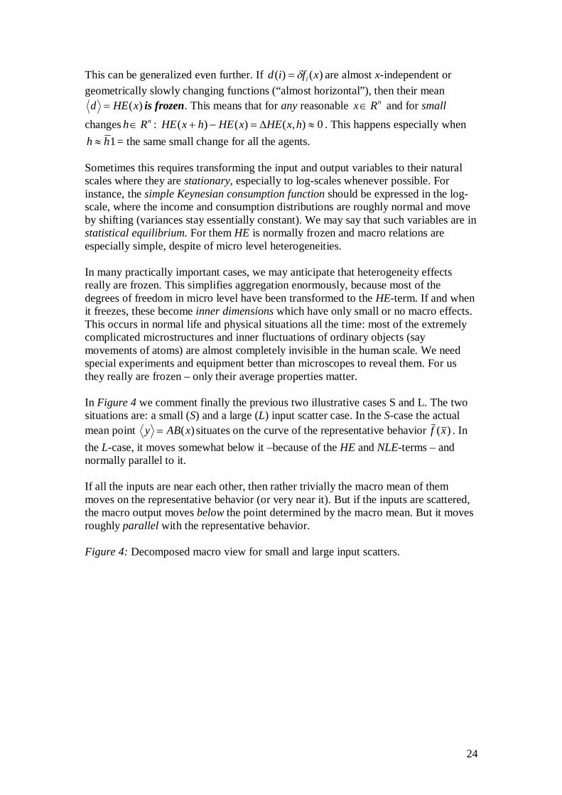
24

This can be generalized even further. If )()( xfid i are almost x-independent or geometrically slowly changing functions (“almost horizontal”), then their mean

)(xHEd is frozen. This means that for any reasonable nRx and for small

changes nRh : 0),()()( hxHExHEhxHE . This happens especially when 1hh = the same small change for all the agents.

Sometimes this requires transforming the input and output variables to their natural scales where they are stationary, especially to log-scales whenever possible. For instance, the simple Keynesian consumption function should be expressed in the log-scale, where the income and consumption distributions are roughly normal and move by shifting (variances stay essentially constant). We may say that such variables are in statistical equilibrium. For them HE is normally frozen and macro relations are especially simple, despite of micro level heterogeneities. In many practically important cases, we may anticipate that heterogeneity effects really are frozen. This simplifies aggregation enormously, because most of the degrees of freedom in micro level have been transformed to the HE-term. If and when it freezes, these become inner dimensions which have only small or no macro effects. This occurs in normal life and physical situations all the time: most of the extremely complicated microstructures and inner fluctuations of ordinary objects (say movements of atoms) are almost completely invisible in the human scale. We need special experiments and equipment better than microscopes to reveal them. For us they really are frozen – only their average properties matter. In Figure 4 we comment finally the previous two illustrative cases S and L. The two situations are: a small (S) and a large (L) input scatter case. In the S-case the actual mean point )(xABy situates on the curve of the representative behavior )(xf . In the L-case, it moves somewhat below it –because of the HE and NLE-terms – and normally parallel to it. If all the inputs are near each other, then rather trivially the macro mean of them moves on the representative behavior (or very near it). But if the inputs are scattered, the macro output moves below the point determined by the macro mean. But it moves roughly parallel with the representative behavior. Figure 4: Decomposed macro view for small and large input scatters.

25

Average behaviour and heterogeneity effects

-1

0

1

2

3

4

5

6

7

8

9

0 1 2 3 4

Input

Out

put

S L

For the shown L-configuration of inputs, HE is small and negative. Also, the NLE-term is negative because of the negative curvature of the representative behavior. But both of them are frozen for small changes and thus )()( xfxABy expressed in the standard but somewhat imprecise notation. But it will communicate the relevant message, that under these conditions the changes of the representative behavior )(xf reflect accurately the changes of the Actual Macro Behavior AB.

Summary The confusion experienced by most of us in these matters shows in our opinion, that we have a long and tedious road in front of us. We have shown one way to proceed along it in order to better understand aggregation questions and their connections to effectively modeling complex micro-macro systems.