what is to expect from the transit method - tu berlin · pdf filewhat is to expect from the...
TRANSCRIPT

What is to expect from the transit method
M. Deleuil, Laboratoire d’Astrophysique de Marseille Institut Universitaire de France
Monday, June 6, 2011

Transit - method
D
D
Transit
No transit
✤ Occurrence: only if the planet orbital plane is close to the observer’s line of sight. The planet must cross over the diameter of the star as we watch it.
Monday, June 6, 2011

Transit - occurrence
✤ Probability of transit occurrence
Monday, June 6, 2011

Transit - occurrence
✤ Probability of transit occurrence
D
ap
Monday, June 6, 2011

Transit - occurrence
✤ Probability of transit occurrence
D
ap
Range of solid angles under which a transit can be observed :
Monday, June 6, 2011

Transit - occurrence
✤ Probability of transit occurrence
D
ap
Range of solid angles under which a transit can be observed :
Transit probability (geometric):
Monday, June 6, 2011

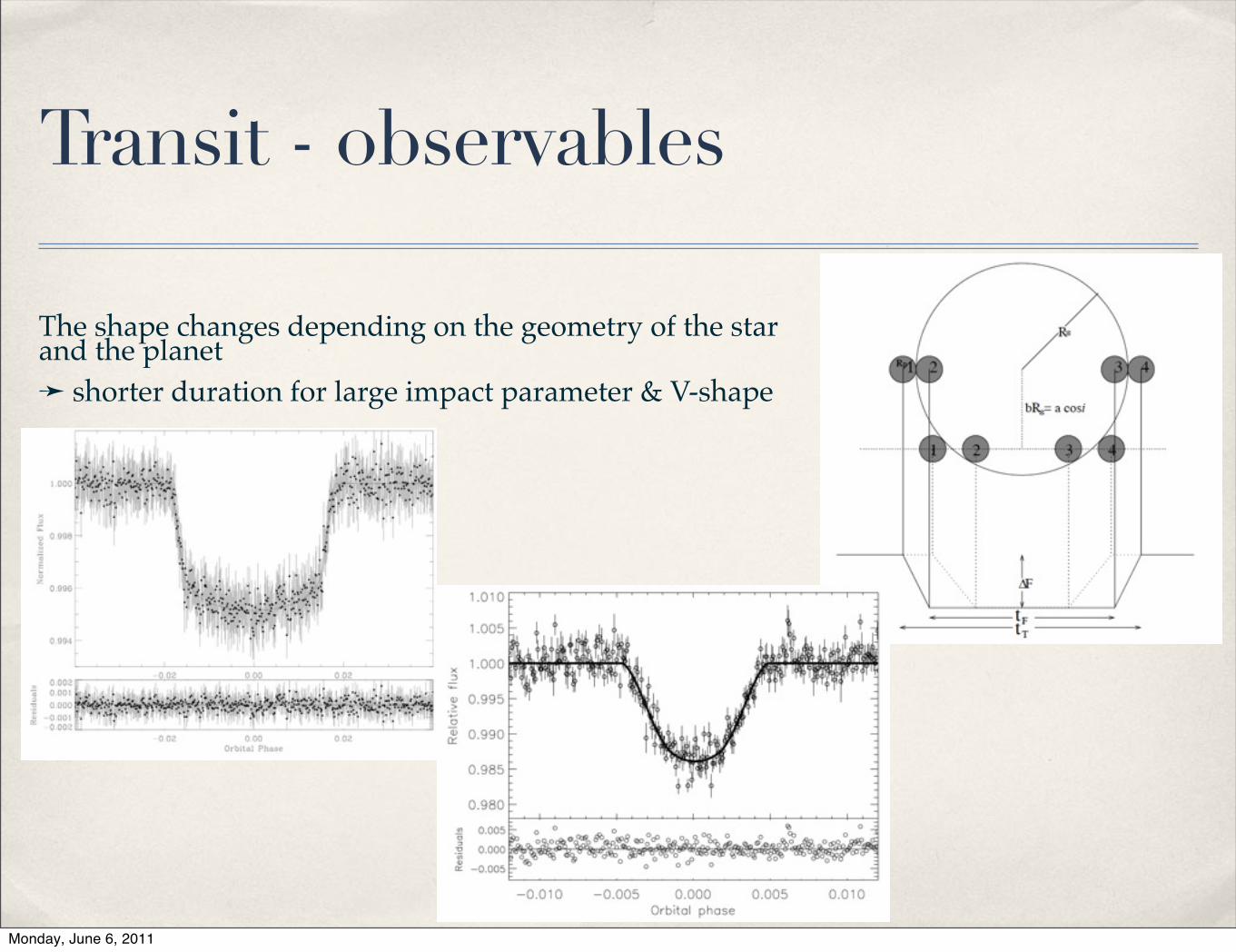
Transit -observables
F0 : out-of transit flux
tc : mid transit timeδ= (F0 - Ftransit)/F0 flux of the photometric decrement during the full phase of the transitΔτ : duration of the ingress or egressΔT : total duration (between the mid point) P : the period
Geometry is described by the transit depth, shape and duration
Monday, June 6, 2011
Transit - observables
The shape changes depending on the geometry of the star and the planet➛ shorter duration for large impact parameter & V-shape
Monday, June 6, 2011

Transit -Physical parameters
Assuming :
• a circular orbit • the planet is dark• a single star • the stellar mass-radius relation is known• the transits have a flat bottoms• the orbital period is known (2 transits at least)
Monday, June 6, 2011

Transit -Physical parameters
Radii ratio
Impact parameter:
Scaled stellar radius :
e orbital eccentricity ; ω argument of pericenter
Seager & Mallen-Ornelas, ApJ 585, 2003; Carter et al., 2008
Physical parameters to be derived from the observables : M✭, R✭, a, i, Rp
Rp
R∗
= δ =ΔFF0
b =ap cos(i)
R∗
= 1− δ Tτ
R∗
a≈π T τδ 1/4 P
1+ esinω1− e2
⎛⎝⎜
⎞⎠⎟
Monday, June 6, 2011

Transit -Physical parameters
➙ mean stellar density
Combined to Kepler’s law
▲ giant star ; ★ dwarf stars
ρ∗ ≈3Pπ 2G
δTτ
⎛
⎝⎜⎞
⎠⎟
3/21− e2
(1+ esinω )2⎡
⎣⎢
⎤
⎦⎥
3/2
➙ useful to help identifying blends and get the star’s radius
Seager & Mallen-Ornelas, 2003 APJ 585, 1038;Southworth et al., 2007, MNRAS 379
Monday, June 6, 2011
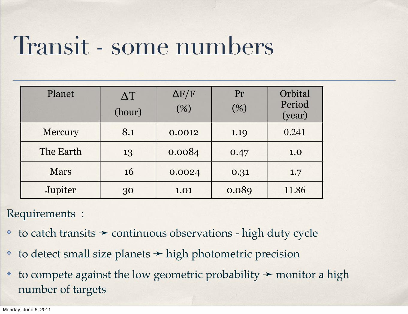
Transit - some numbers
Planet ΔT
(hour)
ΔF/F(%)
Pr(%)
Orbital Period (year)
Mercury 8.1 0.0012 1.19 0.241
The Earth 13 0.0084 0.47 1.0
Mars 16 0.0024 0.31 1.7
Jupiter 30 1.01 0.089 11.86
Requirements :✤ to catch transits ➛ continuous observations - high duty cycle✤ to detect small size planets ➛ high photometric precision✤ to compete against the low geometric probability ➛ monitor a high
number of targetsMonday, June 6, 2011

Transit : issues with the star
✤ the limb-darkening effect : the stellar disk is not uniform
➛ affect the transit shape
➛ depends on the star’s physical parameters (Teff, logg) - color effect
and on the photometric system
Narrow band-width ➛ large effects of stellar limb darkening Smoother edges and U shape bottom ➛ large uncertainties on the transit’s parametersSmoother edges and U shape bottom
Seager & Mallen-Ornelas, ApJ 585, 2003 Pal, 2008 3, 0.8, 0.55, and 0.45µmMonday, June 6, 2011
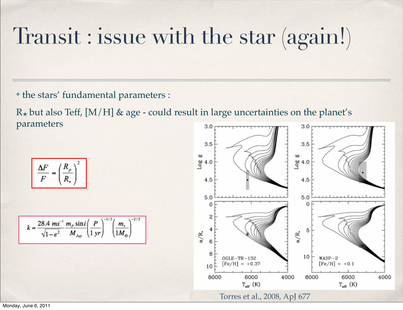
✤ the stars’ fundamental parameters :
R✭ but also Teff, [M/H] & age - could result in large uncertainties on the planet’s parameters
Transit : issue with the star (again!)
Torres et al., 2008, ApJ 677Monday, June 6, 2011

✤ the stars’ fundamental parameters :
R✭ but also Teff, [M/H] & age - could result in large uncertainties on the planet’s parameters
Transit : issue with the star (again!)
Torres et al., 2008, ApJ 677Derived from transit fit
Monday, June 6, 2011

Transits in practice
Observe your stars over a long time lag, perform photometry with the best precision you can achieve, build light curves
Monday, June 6, 2011

Transits in practice
Observe your stars over a long time lag, perform photometry with the best precision you can achieve, build light curves
Monday, June 6, 2011

... get some transits
Perform transit detection with your favorite software
Monday, June 6, 2011

... get some transits
Perform transit detection with your favorite software
Monday, June 6, 2011
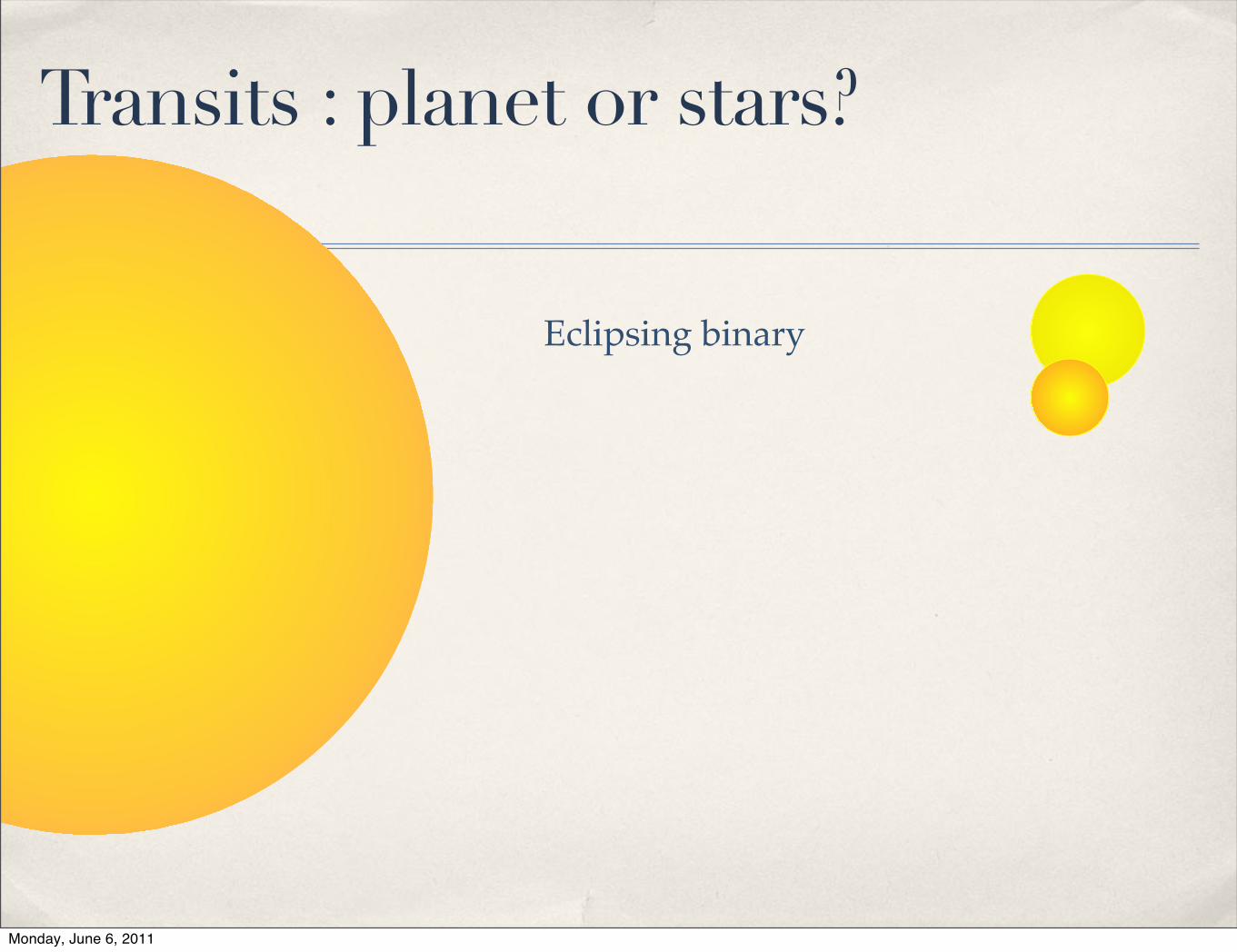
Transits : planet or stars?
Eclipsing binary
Monday, June 6, 2011

Transits : planet or stars?
Eclipsing binary
Monday, June 6, 2011

Transits : planet or stars?
Eclipsing binary
Monday, June 6, 2011

Transits : planet or stars?
Eclipsing binary
mv=13.2P=10.5 d
SB1
Monday, June 6, 2011

Transits : planet or stars?
blends
Check the photometric behavior of the nearby stars
Monday, June 6, 2011
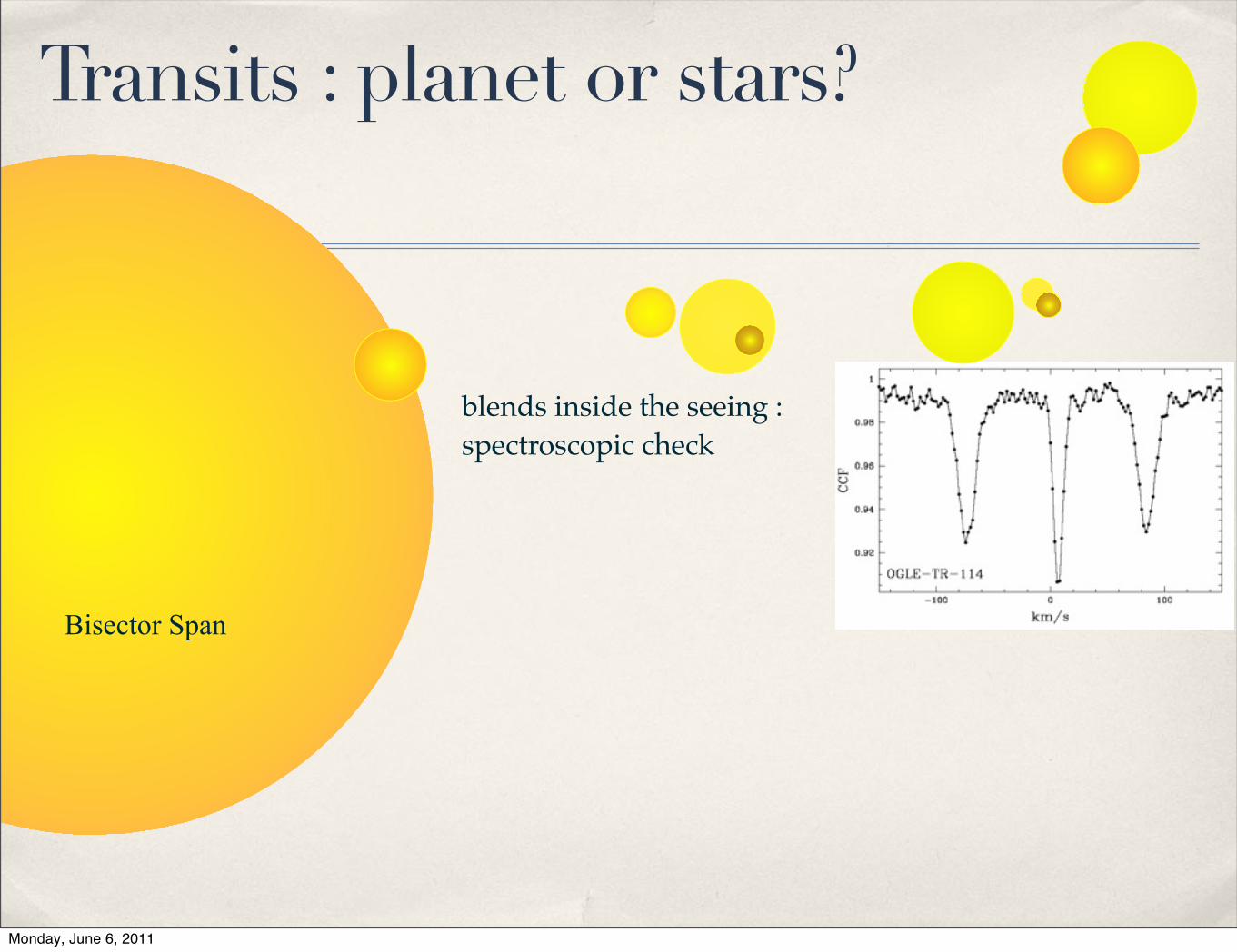
blends inside the seeing : spectroscopic check
Bisector Span
Transits : planet or stars?
Monday, June 6, 2011

blends inside the seeing : spectroscopic check
Bisector Span
Transits : planet or stars?
Monday, June 6, 2011

blends inside the seeing : spectroscopic check
Bisector Span
Transits : planet or stars?
Monday, June 6, 2011

blends inside the seeing : spectroscopic check
Bisector Span
Transits : planet or stars?
Monday, June 6, 2011

blends inside the seeing : spectroscopic check
Bisector Span
Transits : planet or stars?
Amplitude changewith the CCF template
Monday, June 6, 2011

Transits : in practice
Different codes exist to calculate realistic LC e.g. Giménez (2006,A&A 207) on the phase-folded transit determine : the transit center Tc, the orbital phase at first contact θ1, the ratio of radii k, the orbital inclination i and the limb darkening coefficients
or global analysis of the photometry and the radial velocity measurements with Bayesian Markov Chain Monte-Carlo (MCMC) algorithm : the ratio of the radii, the transit width (from first to last contact) W, the transit impact parameter, the orbital period P, the time of minimum light T0, the two parameters √(e) cosω and √(e) sinω where e is the orbital eccentricity and ω is the argument of periastron, and the parameter , where K is the RV orbital semi-amplitude.
K2 = K (1− e2 )P1/3
Aigrain et al., 2008, A&A 448
Monday, June 6, 2011

Transit versus radial velocity
Method transit radial velocity
parameters P, Rp, i Msini, P, e
limitations star’s size; stars’ parameters
slow rotators, stellar activity
bias dwarfs spectral type
Association of the two methods :
• the planet’s fundamental parameters ;
• the complete orbit parameters;
• allow to enlarge the space parameters toward active stars or fast rotatorsMonday, June 6, 2011
Transits : probing planetary systems
Assuming the photometric precision is high enough you can :✤ measure the planetary radius : bring constrains on the planet evolution and migration history and on planet’s composition and atmosphere.
✤ the orbital plane configuration : period, eccentricity, inclination ✤ the planet’s atmospheric properties :
• albedo,• thermal emission, • composition
✤ Stellar surface: limb darkening, spots ✤ Star - planet interactions ✤ Additional unseen companion (TTV) planet or moons✤ Rings and satellites ✤ Oblateness & obliquity
Monday, June 6, 2011

Transits - current situation
Transit
Monday, June 6, 2011

Transits - planet’s nature
123 transiting planets ➛ a striking diversity & the very first secured rocky planets
Monday, June 6, 2011
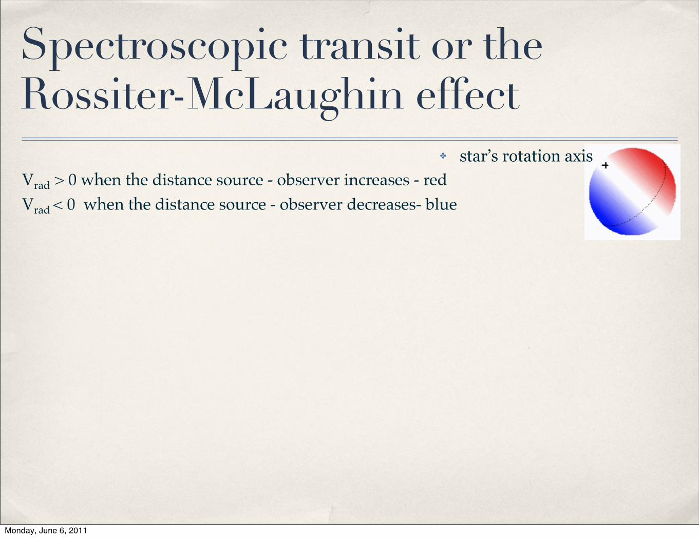
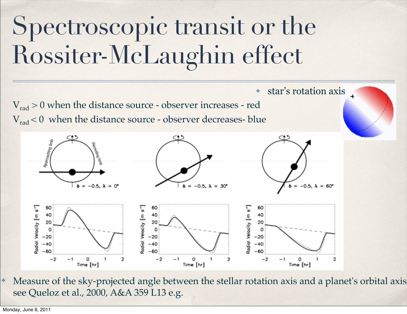
Spectroscopic transit or the Rossiter-McLaughin effect
✤ star’s rotation axisVrad > 0 when the distance source - observer increases - redVrad < 0 when the distance source - observer decreases- blue
Monday, June 6, 2011

Spectroscopic transit or the Rossiter-McLaughin effect
✤ star’s rotation axisVrad > 0 when the distance source - observer increases - redVrad < 0 when the distance source - observer decreases- blue
Monday, June 6, 2011
Spectroscopic transit or the Rossiter-McLaughin effect
✤ Measure of the sky-projected angle between the stellar rotation axis and a planet's orbital axis see Queloz et al., 2000, A&A 359 L13 e.g.
✤ star’s rotation axisVrad > 0 when the distance source - observer increases - redVrad < 0 when the distance source - observer decreases- blue
Monday, June 6, 2011

Spin-orbit : probing the hot Jupiters dynamical origin
766 G. Hébrard et al.: Misaligned spin-orbit in the XO-3 planetary system?
Fig. 2. Phase-folded radial velocity measurements of XO-3 (correctedfrom the velocity Vr = !12.045 km s!1) as a function of the orbitalphase and Keplerian fit to the data. Orbital parameters correspondingto this fit are reported in Table 2. For display purpose all the measure-ments performed during the transit night are plotted here. However, onlythe first four measurements of the transit night are used for the orbitfit, together with 19 measurements secured at other orbital phases (seeSect. 4.1). Figures 5 and 6 display a magnification on the transit nightmeasurements.
Table 2. Fitted orbit and planetary parameters for XO-3b.
Parameters Values and 1! error bars Unit
Vr !12.045 ± 0.006 km s!1
P 3.19161 ± 0.00014 dayse 0.287 ± 0.005" !11.3 ± 1.5 "
K 1.503 ± 0.010 km s!1
T0 (periastron) 2 454 493.944 ± 0.009 BJD!(O ! C) 29 m s!1
reduced #2 0.85N 23tc (transit) 2 454 494.549 ± 0.014 BJDM$ 1.3 ± 0.2 M#R$ 1.6 ± 0.2 R#Mp sin i 12.4 ± 1.9† MJup
i 82.5 ± 1.5 "
Mp 12.5 ± 1.9† MJup
Rp 1.5 ± 0.2 RJup
% 70 ± 15 "
†: using M$ = 1.3 ± 0.2 M#.
than Johns-Krull et al. (2008) from photometric observationsof twenty transits. A 1.5 year time span is obtained when theSOPHIE measurements are fitted with the radial velocities mea-sured by Johns-Krull et al. (2008) using the telescopes HarlanJ. Smith (HJS) and Hobby-Eberly (HET). This longer time spanallows a more accurate period measurement. We obtained P =3.19168 ± 0.00015 days from the fit using the three datasets,in agreement with the photometric one, and with a similar un-certainty. The final period reported in Table 2 (P = 3.19161 ±0.00014 days) reflects these two measurements and is used forthe fits plotted in Figs. 1 and 2. Adding HJS and HET data doesnot significantly change the other orbital parameters or their un-certainties. For the global fit using the radial velocities from thethree instruments, we did not use the last HET measurement,performed during a transit (see Sect. 6).
The Keplerian fit of the new SOPHIE radial velocity mea-surements also improves the transit ephemeris, as the photomet-ric transits reported by Johns-Krull et al. (2008) were secured
Fig. 3. Light curve of XO-3 observed at the Teide Observatory, Tenerife,during the 2008 February 29 transit. The transit fit (solid line) providestc = 2 454 526.4668 ± 0.0026 $ 2 454 494.5507 ± 0.0030 (BJD).
between December 2003 and March 2007, one hundred or moreXO-3b revolutions before the January 28, 2008 transit. Themidpoint of this transit predicted from the Keplerian fit of theSOPHIE radial velocity measurements is tc = 2 454 494.549 ±0.014 (BJD), i.e. just a few minutes earlier than the predictionfrom Johns-Krull et al. (2008). The uncertainty on this transitmidpoint is ±20 min (or ± 0.004 in orbital phase).
To reduce this uncertainty, we observed a recent photo-metric transit of XO-3b with a 30 cm telescope at the TeideObservatory, Tenerife, Spain, on February 29, 2008 (Fig. 3).Weather conditions were poor, so we analyzed the transit witha fixed model based on the algorithm of Giménez (2006b).The fixed parameters were the ratio between the radii of thestar and of the planet k = 0.0928, the sum of the projectedradii rr = 0.2275, the inclination i = 79."3, and the eccen-tricity e = 0.26. We then scanned di!erent mid-transit timesand found tc = 2 454 526.4668 ± 0.0026 (BJD) from #2 vari-ations. This only reflects photon noise; fluctuations due to poorweather may introduce additional uncertainties. By taking theuncertainty on the orbital period into account, this translates intotc = 2 454 494.5507± 0.0030 (BJD) for the spectroscopic transitthat we observed with SOPHIE on January 28, 2008, i.e. ten rev-olutions earlier. That is just two minutes after the above predic-tion from SOPHIE ephemeris, and the uncertainty on this transitmidpoint is ±4.3 min (or ±0.0009 in orbital phase).
4.2. Transit light curve fit revisited
Johns-Krull et al. (2008) point out that the host star radius ob-tained from the spectroscopic parameters (temperature, grav-ity, metallicity), combined with stellar evolution models, R$ %2.13 R#, is incompatible with the value obtained from the shapeof the transit light curve, namely R$ % 1.48 R#. Indeed, a largestellar radius implies a large planetary radius (to account for thedepth of the transit) and a large inclination angle (to accountfor the duration of the transit), but the time from the first to thesecond contacts (ingress) and third to fourth contacts (egress)predicted for such an inclination are too long when comparedto the observed transit light curve (see the upper panel of Fig. 9in Johns-Krull et al. 2008). Formal uncertainties on the stellarspectroscopic parameters and the photometric measurements areinsu"cient to account for the mismatch. Since there can be onlyone value of the real stellar radius, this must be due to systematicuncertainties on the spectroscopic parameters or the parameter
Hébrard et al., 2008, A&A 488, 763
G. Hébrard et al.: Misaligned spin-orbit in the XO-3 planetary system? 769
Fig. 6. Rossiter-McLaughlin e!ect models with ! = 70! and the lowRp value reported by Winn et al. (2008a). The squares (open and filled)are the SOPHIE radial-velocity measurements of XO-3 with 1" errorbars as a function of the orbital phase. Only the first four measurements(filled squares) are used for the Keplerian fit (together with 19 measure-ments at other orbital phases; see Sect. 4.1). The solid and dotted linesare the Keplerian fits with and without the Rossiter-McLaughlin e!ect.
Fig. 7. Residuals of the Rossiter-McLaughlin e!ect fits. Top: withouttransit. Middle: ! = 0! (spin-orbit alignment). Bottom: ! = 70!. Thesquares (open and filled) are the SOPHIE radial-velocity measurementsof XO-3 with 1" error bars as a function of the orbital phase. Only thefirst four measurements (filled squares) are used for the Keplerian fit(together with 19 measurements at other orbital phases; see Sect. 4.1).The vertical, dashed line shows the center of the transit.
velocity dispersion around the model. The best fit with these pa-rameters is plotted in Fig. 6. The residuals are plotted in Fig. 7 inthree cases: without transits, with spin-orbit alignment, and with! = 70!. Among them, the last case is clearly favored by ourdata when the parameters from Winn et al. (2008a) are adopted.
6. Conclusion and discussion
Table 2 summarizes the star, planet, and orbit parameters of theXO-3 system that we obtained from our analyses. The radial ve-locity measurements that we performed with SOPHIE during aplanetary transit suggest that the spin axis of the star XO-3 couldbe nearly perpendicular to the orbital angular momentum of itsplanet XO-3b (! = 70! ± 15!). A schematic view of the XO-3system in this configuration is shown in Fig. 8. We note thatone Johns-Krull et al. (2008) HET measurement was obtainednear a mid-transit of XO-3b. This radial velocity is blue-shiftedby (260 ± 194) m s"1 from the Keplerian curve, in agreement
Fig. 8. Schematic view of the XO-3 system with transverse transit, asseen from the Earth. The stellar spin axis is shown, as well as the planetorbit and the ! misalignment angle (or stellar obliquity). The grey areashows the range ! = 70! ± 15!, which is favored by our observations(see Sect. 5).
with the possible transverse Rossiter-McLaughlin e!ect we re-port here, though with a modest significance.
The SOPHIE observation remains noisy, showing more dis-persion around the fit during the transit than at other phases. Weconsider this result as a tentative detection of transverse transitrather than a firm detection. Indeed, the end of the transit wasobserved at high airmasses, which could possibly biases the ra-dial velocity measurements. Our fits favor a transverse transit,but one cannot totally exclude a systematic error that would bychance mimic the shape of a transverse transit. This would implythat the radial velocities measured during the end of the transitnight, at high airmasses, would be o! by about 100 m s"1, i.e.three to four times the expected errors. Other spectroscopic tran-sits of XO-3b should thus be observed. They will allow the trans-verse Rossiter-McLaughlin e!ect to be confirmed or not and toquantify its parameters better, such as the value of the misalign-ment angle !.
Narita et al. (2008) estimate that the timescale for spin-orbit alignment through tidal dissipation is longer than a thou-sand Gyrs. This timescale is uncertain, but much longer than thetimescale for orbit circularization, which itself is longer than theage of XO-3, estimated in the range 2.4–3.1 Gyr (Johns-Krullet al. 2008). There are thus no obvious reasons to exclude aneccentric, transverse system. A strong spin-orbit misalignmentwould favor formation scenarii that invoke planet-planet scat-tering (Ford & Rasio 2006) or planet-star interaction in a bi-nary system (Takeda et al. 2008) rather than inward migrationdue to interaction with the accretion disk. This suggests in turnthat some close-in planets might result from gravitational in-teraction between planets and/or stars. Chatterjee et al. (2007)and Nagasawa et al. (2008) have recently shown that scatter-ing with at least three large planets can account for hot Jupitersand predicts high spin-orbit inclinations (see also Malmberget al. 2007). On the other hand, XO-3b is an object close to thehigher end of planetary masses. As discussed for instance byRibas & Miralda-Escudé (2007), there are some indications thatthese objects are low-mass brown dwarfs, formed by gas cloud
Monday, June 6, 2011

Spin-orbit : probing the hot Jupiters dynamical origin
• 8 out 26 misaligned ➛ the creation of retrograde planets involves another body: planetary or stellar •Trend with the M★/Teff ➛ planet formation and migration depend on the stars’ mass or the final evolution is linked to the internal structure of the stars, specifically the depth of the outer convective zone
Winn et al., 2010, ApJ
Triaud et al., 2010, A&A
Monday, June 6, 2011

Transits : probing the atmosphere
• planet’s phase variation ➛ albedo•occultation ➛ atmospheric properties
Monday, June 6, 2011

Transits : planet’s atmosphere
CoRoT-1b
Red LC : depth = 0.0126 ± 0.0036% (4σ )T = 2390 K +/- 90geometric albedo < 0.20Snellen et al., 2009, Nature
White LC : Depth = 0.016 ± 0.006% (3.5 σ )Tp = 2330 +120 /-140K Alonso et al., 2009a A&A
CoRoT-2b
CoRoT-2b White LC : Depth = 0.006 ± 0.002%Tp = 1910 +90 /-100K geometric albedo < 0.12Alonso et al., 2009b A&A
CoRoT-1b : optical phase variation
Monday, June 6, 2011
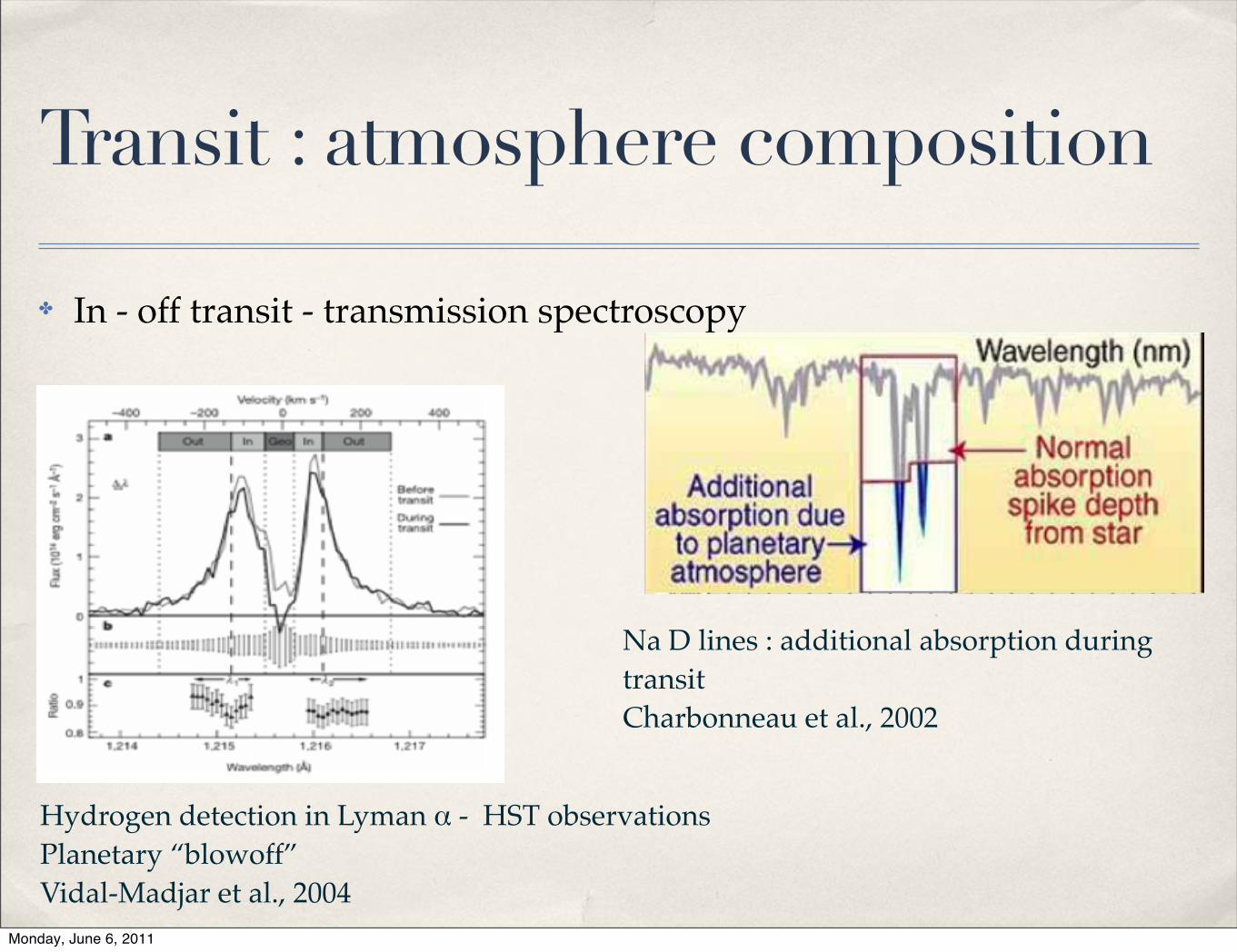
Transit : atmosphere composition
✤ In - off transit - transmission spectroscopy
Hydrogen detection in Lyman α - HST observationsPlanetary “blowoff”Vidal-Madjar et al., 2004
Na D lines : additional absorption during transitCharbonneau et al., 2002
Monday, June 6, 2011

Transit : atmosphere composition 2– 11 –
Fig. 2.— Comparison of the measured wavelength dependent planet-to-star radius ratios totransmission spectroscopic models from Miller-Ricci & Fortney (2010). The two radius ratios
obtained from the Spitzer observations are the black filled circles with their 1 ! error bars.The results from MEarth and VLT observations are shown as black square and triangles,
respectively. The continuous lines correspond to the best-scaled and smoothed transmissionspectra expected from model of GJ 1214b atmosphere’s (Miller-Ricci & Fortney 2010). Thered continuous line corresponds to a transmission spectra with solar composition (H/He
rich), the red dotted lines is the same spectra but with metallicity enhanced by a factor of50. The green line is a model with solar composition but with no methane and the blue line
is a model with 100% water vapor in the atmosphere. The open circles are the flux weightedintegrated models in the Spitzer bandpasses. The dotted black lines at the bottom of the
plot correspond to the instrumental bandpasses. The hydrogen rich model (red continousline) is ruled out a 7 ! level by the combined set of observations.
We thank Bryce Croll, Heather Knutson, Dimitar Sasselov, Nadine Nettelmann and
Leslie Rogers for useful discussions. This work is based on observations made with the SpitzerSpace Telescope which is operated by the Jet Propulsion Laboratory, California Institute ofTechnology under a contract with NASA. We thank the Sagan Fellowship Program, which
provides support for JB and EK.
GJ1214b Mp = 6.55 +/- 0.98 MJup Rp = 2.68 +/- 0.13 REarth star : M4Vat 3.6 and 4.5 microns with Spitzerflat transmission spectrum over the large wavelength domain ➛cloud-free, metal rich atmosphereDésert J.-M. et al., 2011, ApJ 731
Monday, June 6, 2011

Transits : timing variation induced by an additional planet
Csizmadia priv. com.
Agol, E. et al., 2005, MNRAS, 359, 567Monday, June 6, 2011
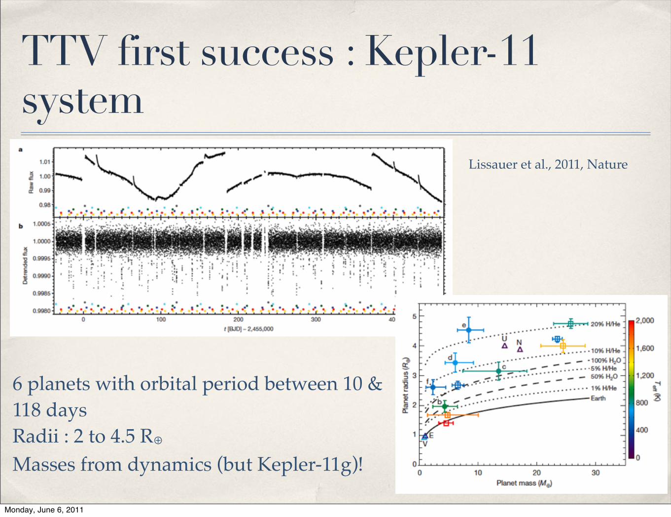
TTV first success : Kepler-11 system
Lissauer et al., 2011, Nature
6 planets with orbital period between 10 & 118 days Radii : 2 to 4.5 R⊕
Masses from dynamics (but Kepler-11g)!
Monday, June 6, 2011

Probing the star’s surface and understanding the star’s activity
✤ stellar spots leave their imprints on the transits • Rp/R★ = 0.172 (3% larger)
• Average of 7 spots covered per transit• spot size : 03 - 0.6 Rp• Temperature : 4600 to 5400 K (R★ =5625K)
• rise & decay ~ 30 days
Czesla et al., 2009, A&A 505Wolter et al., 2009, A&A 504 Silva-Valio et al., 2010, A&A 510
Monday, June 6, 2011

Moons, rings & others
P. Sartoretti and J. Schneider: Satellites of extrasolar planets 559
Fig. 4. Examples of transit lightcurves (see text for interpreta-tion). a) For a planet with rp = rJ and TP = 50days and asatellite with rs = 2.5rE and TS = 0.5 days. b) For a planetwith rp = rJ and TP = 50days, alone. c) For a planet withrp = rJ and TP = 50days and a satellite with rs = 2.5rE andTS = 1.5 days. d) For a smaller planet with rp = 2.5rE andTP = 100 days and a satellite with rs = 1.5rE and TS = 2days.In all panels the solid line is the model lightcurve, and thecrosses show the results of simulated 10 min exposure observa-tions with a poisson noise of 10!4
stars. All feature of the lightcurve are mapped faithfully.In particular, the planet-satellite transit is detected witha signal-to-noise ratio of order 10. For reference, Fig. 4bshows the transit lightcurve of the same planet but with-out a satellite.
If the satellite period does not satisfy condition (23) forat least one planet-satellite transit, the probability for thesatellite to pass through one of the two favorable conjunc-tions that will produce a transit during the time intervalDT is simply given by NPS. As shown above, the probabil-ity will be highest for satellites with smallest orbital radii.
The Moon, for example, has TS ! 0.15T1/3P and ! " 6,
and it would have a probability of only 0.04 to be observedin a transit over or behind the Earth during a transit ofthe planet over the Sun.
Figure 4c shows the transit lightcurve of the sameplanet as in Fig. 4a, but with a satellite with rs = 2.5rEand TS = 1.5 days, which does not satisfy condition (23).
The abrupt drop of the stellar flux at the beginning ofthe transit is caused by the entry of the planet. The pro-nounced, but more moderate drop at t " 0 hr is caused bythe subsequent entry of the satellite. Then, the planet firstleaves the star causing the flux to increase sharply. Thesatellite continues to occult the star from about t = 3.5to 4.5 hr until it finally also leaves, and the stellar fluxretrieves its original value. Again, the crosses show theresults of simulated 10 min exposure observations with apoisson noise of 10!4. For comparison, we show in Fig. 4dthe transit lightcurve for a smaller planet with rp = 2.5rEand TP = 100 days and a satellite with rs = 1.5rE andTS = 2days. The characteristic signatures of the entryand exit of first the planet and then the satellite are sim-ilar to those in Fig. 4c. Although the signal-to-noise levelis about 4 times smaller than in Fig. 4c, the satellite andplanet transits are still detected unambiguously.
4. Indirect detection by timing of the planet transits
If a satellite is not extended enough to produce a de-tectable signal in the stellar lightcurve, it may still bedetected indirectly through the associated rotation of theplanet around the barycenter of the planet-satellite sys-tem. This requires that a planetary transit be observed atleast 3 times, as the e!ect of the rotation will be a peri-odical time shift of the lightcurve minima induced by theplanet transits. We now estimate the expected time shiftin the simple case where the satellite and planet orbitalplanes are aligned along the line of sight (ips " ip " 0).In this case, the projected diameter of the planet orbitaround the barycenter of the planet-satellite system is2asMsM!1p , whereMs is the satellite mass. Therefore, theexpected time shift between transits will be
"t # 2asMsM!1p $ Tp(2"ap)!1 . (24)
Measurements of "t, in addition to revealing the pres-ence of a satellite, provide also an estimate of the productof its mass and orbital radius, asMs. The minimum de-tectable asMs is determined by the the minimum measur-able time shift, and hence, by the accuracy of the timingof lightcurve minima. If #tobs denotes the sampling time,i.e., the duration of each consecutive exposure, then wecan expect to be sensitive to the presence of satellites with
Msas #Mpap"#tobs/Tp . (25)
We have estimated the minimum sampling time re-quired to determine the position of a lightcurve minimumwith a timing accuracy of #tobs. We simulated observedlightcurves using di!erent values of #tobs and consider-ing poisson noise only, which we cross-correlated with thecorresponding input model lightcurves. We find that theminimum #tobs required corresponds to the exposure timeneeded to detect the depth of the planetary transit min-imum at twice the photon noise level, i.e., |"F"| > 2$(see Eq. (1)). As an example, the minimum #tobs would
Theoretical study :Sartoretti & Schneider 1999, A&A
direct measure of the transit of a moon1350 F. Pont et al.: Hubble Space Telescope times-series photometry of HD 189733
Fig. 1. Decorrelated lightcurve phased to P = 2.218581 days, with best-fit model transit curve. Top: flux after external parameter decorrelation as afunction of phase; Bottom: residuals around the best-fit transit model. Light blue for the first visit, dark blue for the second and green for the third.Open symbols indicate data a!ected by Features A and B (see text), not used in the fit. Dotted lines show the±10!4 level.
also seen in the zeroth-order image on the CCD. It is accompa-nied by a detectable change of spectral distribution, which sug-gests an explanation in terms of the transiting planet occulting acool spot on the surface of the star (see Sect. 4.5).
Feature B is also larger than instrumental e!ects, and doesnot correlate with any of our external instrumental parameters.Its less regular shape and the fact that any colour e!ect is belowthe noise level indicate that, in principle, an explanation in termsof instrumental noise cannot be entirely excluded. Based on ourexperience with previous HST high-accuracy times series, andthe simulations of Sect. 3.3, we believe, however, that Feature Bis also real.
We do not use Features A and B in the analysis of thelightcurve in terms of planetary transit. They are treated sepa-rately in Sect. 4.5.
4.2. Stellar activity and variability
HD 189733 is an active star, variable to the percent level. Itis listed in the Variable Star Catalogue as V452 Vul. A chro-mospheric activity index of S = 0.525 has been measured byWright et al. (2004). Activity-related X-ray emissivity has beenmeasured by both EXOSAT and ROSAT, activity-related radialvelocity residuals of 15 m s!1 were reported by Bouchy et al.(2005). Winn et al. (2007) have measured the photometric vari-ability of this star extensively and confirm variability at thepercent level, compatible with an explanation in terms of tran-sient spots modulated by a rotation period of Prot " 13.4 days.Moutou et al. (2007) measure strong activity in the CaII lineand infer a strong magnetic field with a complex topology fromspectropolarimetric monitoring. The explanation of Features Aand B in terms of starspots is therefore natural. The presenceof large starspots is also confirmed by an observing campaign
on this object by the MOST satellite (Croll et al., in prep.). TheMOST data yield an improved rotation period of 11.8 days.
The Winn et al. (2007) photometry is contemporaneous withour HST data. Our absolute measurements are placed within thecontext of the ground-based monitoring in Fig. 2, with an ar-bitrary zero-point shift. The HST data is in agreement with theperiodic variation seen in the long-term lightcurve. If we inter-pret this variability in terms of starspots moving in and out ofview with the rotation of the star, then the third visit occurs nearthe brightest point – with less star spots visible – and the firstvisit with a 0.007 dimming due to starspots. The phasing andamplitude of features A and B are perfectly compatible with anexplanation in terms of the planet occulting part of the starspotsresponsible for the photometric variation (see Sect. 4.5).
Before fitting a transit signal, we correct for the variationsof the total stellar luminosity due to the presence of starspots.Outside of features A and B, the planet crosses a spot-free re-gion, therefore a region slightly brighter than the average overthe stellar disc, which includes the spots. This is a tiny correc-tion of the scaling between transit depth and radius ratio (of theorder of 2 # 10!4 in flux). Nevertheless, to the level of the ac-curacy of the HST lightcurve, it makes a significant di!erenceand must be accounted for. We use the absolute flux di!erencesmeasured in Sect. 3.4.
4.3. Transit signal
A transit light curve computed with the Mandel & Agol (2002)algorithm was fitted to the light curve, with a downhill simplexalgorithm (Press et al. 1992). Features A and B were removedwith cuts from JD = 877.875 to the end of orbit 3 of visit 1,and from the beginning of orbit 3 of visit 2 to JD = 882.333.The limb-darkening coe"cients were left as free parameters,
Test on HD 189733 : moon or rings but a large spot complex (> 80 000km)Pont et al., 2007, A&A 476
Monday, June 6, 2011

Moons, rings & others
5
FIG. 4.— Variations in the transit light curve due to an oblate, oblique, precessing exoplanet. Plotted are the transit depth (!), total duration (Tfull) and ingressduration (" ) fractional variations (T!V, TDV, and T"V, respectively) that are expected for a uniformly precessing Saturn-like planet around a Sun-like star. Thetime scale is based on the assumption Porb = 17.1 days.
that f and ! cannot be determined independently, althoughEqn. (14) could be used to place a lower bound on f . Thedegeneracy is illustrated in Fig. (5).To break the parameter degeneracy, one possibility is to ar-
range for high-cadence, high-precision observations of at leastone transit, seeking the slight oblateness-induced anomaliesthat were described by Seager & Hui (2002) and Barnes &Fortney (2003). Observations of a single light curve wouldlead to constraints on the sky-projected oblateness and obliq-uity [see Eqns. (7) and (8)], which, together with the T"Vsignal, would uniquely determine f and !. The best time toschedule such observations would be near a minimum of theT"Vcurve, when the light curve anomalies are largest.This would be a challenging task, as the amplitude of
the differences between the actual light curve and the best-fitting model of the transit of a spherical planet would be!100 ppm. For this specific example, even Kepler photom-etry (with 1 min cadence) would be insufficient to detect theanomalies in a single transit. By observing 10 transits nearthe minimum of the T"V signal (during which time the sky-projected quantities are constant to within 1%), Kepler coulddetect the signatures of oblateness and obliquity at the 1#level, but the resulting constraints would be weaker than theconstraints determined by an analysis of the T"Vsignal. Asignificantly larger planet, or brighter host star, would be re-quired for meaningful constraints.Another possibility is to enforce additional physically-
motivated relationships between parameters. In particular, wehave already shown that the precession period is a function ofk, f , !, C and J2 [by combining Eqn. (2) with Eqn. (11)]. Afurther condition can be imposed on f , C and J2, such as theDarwin-Radau approximation for planets in hydrostatic equi-librium (Murray & Dermott 2000):
J2
f= !
3
10+5
2C!
15
8C2. (17)
Following this path, there are 8 model parameters (k, f , !,i, Pprec, $0, C, J2) with 2 physically-motivated constraints
among them. However there are only 5 quantities that are
well determined from the photometric data [Pprec, $0, f sin2 !,
k2(1 ! f ), i], leaving us still short by one observable or con-straint from being able to determine all the parameters. Forexample, if one were willing to assumeC = 0.23, then we findfrom our simulated Kepler data that f , !, J2 and Pprec can berecovered with a precision of about 10%, and k is recoveredwithin 1%.Assigning C a specific value is unrealistic, but for realis-
tic planets one expects C to be smaller than 0.4 (Murray &Dermott 2000). We repeated the analysis of our hypotheti-cal T"Vsignal, allowingC to be a free parameter restricted tothat range, with a uniform prior.1 In effect we averaged theresults over a range of C deemed to be physically plausible.As might be expected, a strong degeneracy was observed be-tween f and !, as seen in Fig. (5). However, we were still ableto determine J2 to within 10%, and k to within 2%.
5. DISCUSSION
In this paper we have investigated the observability ofchanges to transit light curves resulting from the spin pre-cession of an oblate, oblique exoplanet. The most readilydetectable signal is the T"Vsignal, the variation in transitdepth due to the changing area of the planetary silhouette.The planets that seem most likely to exhibit detectable effectsare those with periods between 15–30 days (around Sun-likestars), which is short enough for precession periods to be 40 yror less, and long enough to hope that tidal spin-orbit synchro-nization has not taken place.It is also important to consider other physical processes that
could give rise to T"V signals, and which might confoundthe interpretation of the data. Starspots and other types ofstellar variability can produce transit depth variations. Thesecan be recognized and taken into account by monitoring thestar outside of transits, as is done automatically by the Kepler
1 We also required J2 > 0, which corresponds to C > 0.133 according tothe Darwin-Radau relation (Eqn. 17).
Measure of the planet’s oblateness & spin precession Carter et al., 2011, ApJ 730
Precession of an oblate oblique planet causes changes in the depth and duration of transits
Saturne oblateness : 200 ppm and 2 ppm for a synchronized hot Jupiter
Monday, June 6, 2011

Conclusions
✤ Transits : a powerful tool for characterizing planetary systems :
fundamental parameters, orbit configuration .. ➛ constraints for their formation mechanism(s) and evolution
✤ Observations of bright targets are now required!
✤ Allow to enlarge the space parameters and to start physics studies
✤ Objectives : toward the small size planets and the long orbital periods
Monday, June 6, 2011