Munich Personal RePEc Archive

What is the SARB’s inflation targeting

policy, and is it appropriate?

Ellyne, Mark and Veller, Carl

University of Cape Town

30 August 2011

Online at https://mpra.ub.uni-muenchen.de/42134/

MPRA Paper No. 42134, posted 23 Oct 2012 19:27 UTC

(PRELIMINARY DRAFT)

what is the sarb’s inflation targeting policy,

and is it appropriate?

Carl Veller† and Mark Ellyne††

August 2011

Abstract

Since its adoption of inflation targeting in 2000, the South African Reserve Bank

has been accused of placing too great an emphasis on meeting its inflation target,

and too small an emphasis on the high rate of unemployment in the country. On

the other hand, the SARB has regularly missed its inflation target. We attempt to

characterise the SARB’s inflation targeting policy by analysing the Bank’s interest

rate setting behaviour before and after the adoption of inflation targeting, making

use of Taylor-like rules to determine whether the SARB has emphasised inflation,

the output gap, the real exchange rate, and asset price deviations in its monetary

policy. We find that the SARB has significantly changed its behaviour with the

adoption of inflation targeting, and show that the SARB runs a very flexible inflation

targeting regime, with strong emphasis on the output gap. Indeed, we find evidence

that the emphasis on inflation is too low, and potentially conducive to instability in

the inflation process.

JEL classification: E52, E58

Keywords: South Africa, monetary policy, inflation targeting

Authors’ e-mail: carl.veller@gmail.com, mark.ellyne@uct.ac.za

For presentation at the Biennial Conference of the Economic Society of South Africa,

University of Stellenbosch, 5-7 September 2011.

†Graduate student, Department of Mathematics and Applied Mathematics, University of Cape Town††Adjunct Associate Professor, Department of Economics, University of Cape Town

1 Introduction

Following a growing host of countries, South Africa adopted inflation targeting in 2000,

explicitly making the goal of low and stable inflation the primary objective of monetary

policy. Since then, the regime has received a substantial amount of criticism, with the most

persistent critic, the Congress of South African Trade Unions (COSATU), complaining that

too strict a focus on price stability has come with the cost of higher unemployment, lower

growth and an unstable exchange rate. Supporting their call for a review of the mandate

of the South African Reserve Bank (SARB) is Nobel laureate Joseph Stiglitz, who, in an

article entitled ‘The Failure of Inflation Targeting’, dismisses inflation targeting in general

as a ‘crude recipe . . . based on little economic theory or empirical evidence’ (Stiglitz, 2008).

Such criticisms prompt a number of questions. Has inflation targeting been successful

in other countries? What exactly is the SARB’s inflation targeting policy, and has it been

successful? Does the SARB place an overriding emphasis on meeting its inflation targets,

as COSATU claims, or does it have other objectives as well? Has inflation in fact been

successfully stabilised in South Africa? This paper seeks to address these questions by

analysing the conduct and results of South African monetary policy before and after the

adoption of inflation targeting. Specifically, we compare a ‘pre-inflation targeting’ (pre-IT)

period of 1990Q1-1999Q4 with the inflation targeting (IT) period of 2000Q1-2011Q1.

Broadly, our results suggest that the above criticisms are unfounded. Under inflation

targeting, the SARB has exercised a large degree of flexibility in conducting monetary

policy, with strong consideration shown to real economic variables such as the level of

output. In fact, we argue that the emphasis placed on inflation in this period has been too

low, and has been conducive to the substantial volatility in the inflation rate experienced

over the period.1 There are theoretical reasons for believing this to be the case, and

our estimates of the weight the SARB has accorded inflation in its instrument setting

behaviour in the IT period are significantly lower than corresponding estimates obtained

for other countries in separate studies.

We give evidence that, unlike in the pre-IT regime, under inflation targeting the SARB

has paid little attention to the real exchange rate and other asset prices in their own right.

This suggests a significant simplification of monetary policy over the pre-IT regime, which

is known to have focussed on more eclectic targets (Aron and Muellbauer, 2007). We argue

that the decreased focus on the exchange rate and other asset prices has not necessarily

led to their becoming more volatile, and that inflation targeting, if properly implemented,

can provide a unified framework with which to achieve stability both in these variables

and in inflation.

The paper proceeds as follows: Section 2 briefly outlines the theory and workings

of inflation targeting. Section 3 discusses the international evidence for the success of

inflation targeting as a monetary regime. Section 4 describes and compares the monetary

regimes in South Africa since the mid-1980s. Section 5 is a discussion and estimation of

the SARB’s instrument reaction behaviour using Taylor-like rules. Section 6 concludes.

1It is noteworthy, for example, that a regime that emphasises keeping inflation within a relatively widetarget band has only managed to do so in 19 of the 37 quarters since the year for which the targets werefirst aimed to be achieved (2002).

1

2 The theory of inflation targeting

2.1 Why worry about inflation?

A low and stable rate of inflation is accepted as a central goal of monetary policy for a

number of reasons:

• High inflation tends to depress savings and investment. High inflation is associated

with substantial inflation volatility, which causes uncertainty in price-level expec-

tations, making long-term economic decision-making more difficult (Freedman and

Laxton, 2009). This uncertainty can also complicate labour negotiations, a problem

with particular relevance to South Africa with its highly unionised labour market.

• High inflation distorts relative prices. Whenever firms’ price changes are not synchro-

nised, relative prices will not reflect relative costs of production, distorting consumer

choices and leading to welfare losses (Sørensen and Whitta-Jacobsen, 2005, chap.

20).

• High inflation disproportionately affects the poor. While individuals can in principle

hedge against inflation through the use of inflation-linked financial instruments, these

instruments tend not to be available to the poor, who hold a large portion of their

wealth in the form of inflation-exposed cash (Romer and Romer, 1998; Easterly and

Fischer, 2001).

• High inflation has a distortionary effect on unindexed accounting measures and taxes.

Inflation causes returns to nominal assets to be overtaxed relative to real assets, and

therefore distorts investment decisions (Sørensen and Whitta-Jacobsen, 2005, chap.

20). In addition, if income tax brackets do not move while inflation increases nominal

incomes, individuals could move into higher tax brackets despite their real incomes

not having changed.

2.2 The need for a nominal anchor

Accepting low inflation as a primary goal of monetary policy, central banks typically rely

on a nominal anchor to steer policy decisions. The central bank’s pledge to keep a chosen

nominal variable constant or within specified boundaries helps to clarify the objective of

the central bank’s policy, both within the central bank and to the public, to provide a

publicly visible goal according to which the central bank can communicate any changes

in policy and their rationales, and to guide public expectations with respect to the policy

goal, and subsequently other variables as well.

2.3 What is inflation targeting?

Broadly speaking, inflation targeting involves taking the inflation rate as the nominal

anchor and creating a policy response ‘function’ to manage it. However, inflation targeting

is more than an instrument response rule for managing monetary policy - it has evolved

into a framework with several key elements (Bernanke and Mishkin, 1997; Miao, 2009):

2

• Inflation target identification. The authorities publicly announce a medium-term

inflation target as a point or band. They acknowledge that low, stable inflation is

the primary goal of monetary policy.

• A clear transparency framework. High levels of transparency through communication

with the public regarding goals, plans and decisions of the monetary authority. The

authorities typically publish regular reports stating the inflation targets and steps

being taken to attain them.

• An accountability framework. The monetary authorities are held responsible for

achieving their stated objectives and generally must answer to the government for

any failure to achieve them.

• Appropriate institutional arrangements. The central bank needs to be independent

and credible to achieve its goals. To implement an inflation targeting regime also

requires a sufficiently developed financial market and stable relationships among

financial variables and economic behaviour.

• A policy rule that guides the choice of targets and instruments to manage monetary

policy.

The targeting and instrument rules are not mutually exclusive. A targeting rule spec-

ifies the target variables and their desired levels, usually with reference to minimising an

economic loss function of the general form

L =

τ∑

t=0

[V (πt) + β1V (z1t) + β2V (z2t) + . . .)] ,

where πt is some measure of inflation, the zit are other variables (such as output, the

exchange rate, etc.), V (·) is a function that captures deviations from target levels, and the

βi are subjective weights.

Instrument rules, on the other hand, express the setting of the policy instrument, usu-

ally a short term interest rate, as a function of predetermined or forward-looking variables.

Such rules are typified by the Taylor Rule (Taylor, 1993), under which the monetary au-

thority changes the interest rate linearly in response to changes in inflation and the output

gap:

it = i∗ + φπ(πt − π∗) + φyyt,

where it is the nominal interest rate, i∗ is its (constant) equilibrium level (consistent with

inflation at its target and a zero output gap), π∗ is the inflation target, yt is the output

gap, and φπ and φy are subjective weights. Since current policy decisions affect inflation

with a lag, the inflation variable often becomes forecasted/expected future inflation: the

central bank forecasts a path for inflation to be used as an intermediate target, and selects

an instrument path to coincide with that target at some horizon (Svensson, 2000). In more

general forms, additional variables enter on the right hand side, so that monetary policy

reacts to changes in these variables as well.

The instrument rule should not be interpreted as a mechanical prescription for mone-

tary policy, but rather as guide, as well as a tool for ex-post description (Taylor, 1993).

3

2.4 Strict vs flexible inflation targeting

An important distinction exists between strict and flexible inflation targeting. Strict infla-

tion targeting allows only inflation to enter the monetary authority’s objective function,

so that the sole objective of monetary policy is the stability of inflation. Flexible inflation

targeting, on the other hand, permits other variables such as output to have a nonzero

weight in the objective function; their stability is a goal of monetary policy as well.

Allowing other variables to enter a central bank’s objective function can be reconciled

with the bank’s primary goal of meeting an inflation target if there is a stated horizon over

which the inflation target must be achieved. This gives the central bank time to address

issues other than inflation, while still being able to meet its medium-term inflation target.

Further flexibility may be allowed if the target is a band rather than a point (as in the

case of South Africa), or if there is a ‘tolerance band’ around the point target (as there is

for most inflation targeters).

The SARB has been accused of running an inflexible inflation targeting regime, fo-

cussing too much on inflation stability at the cost of lower growth and an unstable ex-

change rate. In the later empirical analysis, we shall interrogate this claim. As Svensson

(2010) notes though, all inflation targeters exercise some degree of flexibility.

2.5 How inflation targeting works

The success of inflation targeting’s ability to smooth the business cycle in response to

a shock in the economy depends fundamentally on whether the shock comes from the

demand or supply side of the economy. A negative demand shock depresses output while

simultaneously causing a decrease in inflation. The correct interest rate response under an

inflation targeting framework is to decrease rates, the effect of which is to increase inflation

and output back towards desired levels, a result referred to by Blanchard and Galı (2007)

as a ‘divine coincidence’.

Supply shocks present a greater challenge to inflation targeters. A negative supply

shock, such as a sharp increase in the oil price, increases prices while simultaneously

decreasing output. A policy that responds simply to immediate changes in the inflation

rate would raise interest rates, but this would put further strain on flagging output. This

is the type of situation Stiglitz (2008) has in mind when he brands inflation targeting as a

rule decreeing that ‘whenever price growth exceeds a target level, interest rates should be

raised . . . regardless of the source of inflation.’ Of course, this and many other criticisms

of inflation targeting attack a straw man, since all inflation targeters exercise a degree of

flexibility and tend to focus on target horizons. If the monetary authority believes the

supply shock is temporary, they might be inclined to keep interest rates constant (or even

to decrease them) if their forecast of medium-term inflation is still around the inflation

target. Furthermore, flexible inflation targeters do place weight on fluctuations in output

and employment in addition to inflation; the medium-term nature of the inflation target

gives the monetary authority time to concentrate on the stability of these variables as well.

The temporary ‘first-round’ effect of a supply shock can flow through into inflation

expectations and wage- and price-setting, the so-called ‘second-round’ effects of the supply

shock. Since these second-round effects do influence medium-term inflation projections,

an inflation targeting regime must respond to them. Thus, the decision of whether or

4

not to respond to supply-side shocks, such as oil price shocks, can be a complex one,

and may trigger an immediate or delayed response (Cuevas and Topak, 2009). Vigorous

communication with the public by a credible central bank, emphasising the temporary

nature of the supply shock and the bank’s unchanged outlook for core inflation, can help

to contain inflationary expectations and therefore second-round effects as well.

3 International experiences of inflation targeting

Inflation targeting was initially adopted in the early 1990s by industrialised countries such

as New Zealand, Canada and the United Kingdom. Later, a number of emerging economies

also adopted this regime. It is not an insignificant observation that no country that has

adopted inflation targeting has subsequently discarded it; as Rose (2007) points out, such

endurance is a rarity in the world of monetary policy, where regimes have historically not

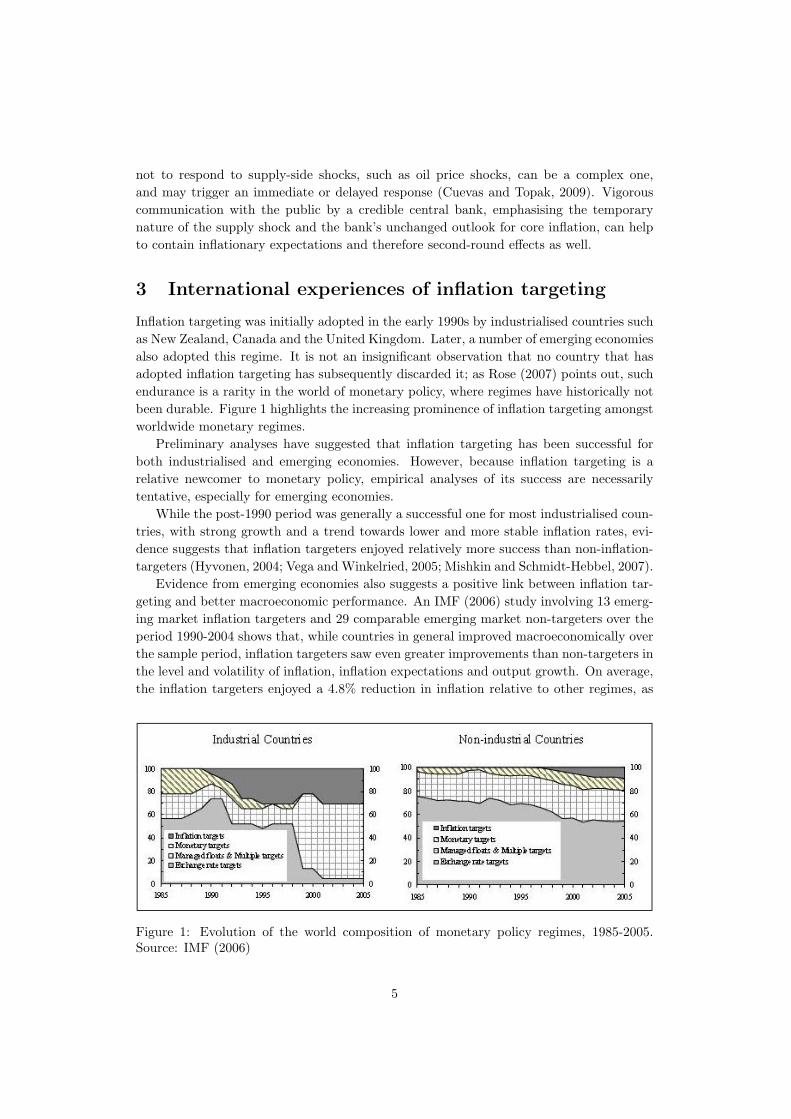
been durable. Figure 1 highlights the increasing prominence of inflation targeting amongst

worldwide monetary regimes.

Preliminary analyses have suggested that inflation targeting has been successful for

both industrialised and emerging economies. However, because inflation targeting is a

relative newcomer to monetary policy, empirical analyses of its success are necessarily

tentative, especially for emerging economies.

While the post-1990 period was generally a successful one for most industrialised coun-

tries, with strong growth and a trend towards lower and more stable inflation rates, evi-

dence suggests that inflation targeters enjoyed relatively more success than non-inflation-

targeters (Hyvonen, 2004; Vega and Winkelried, 2005; Mishkin and Schmidt-Hebbel, 2007).

Evidence from emerging economies also suggests a positive link between inflation tar-

geting and better macroeconomic performance. An IMF (2006) study involving 13 emerg-

ing market inflation targeters and 29 comparable emerging market non-targeters over the

period 1990-2004 shows that, while countries in general improved macroeconomically over

the sample period, inflation targeters saw even greater improvements than non-targeters in

the level and volatility of inflation, inflation expectations and output growth. On average,

the inflation targeters enjoyed a 4.8% reduction in inflation relative to other regimes, as

Figure 1: Evolution of the world composition of monetary policy regimes, 1985-2005.Source: IMF (2006)

5

well as an average 3.6% reduction in the standard deviation of inflation. These results

are shown to be robust to a number of sensitivity tests, including removing countries that

adopted inflation targeting with very high (> 40%) inflation rates. This addresses Ball

and Sheridan’s (2005) objection that empirical analyses such as those cited above often

simply reflect ‘regression to the mean’.2

4 South African monetary policy

4.1 Monetary regimes since the mid-1980s

South Africa has, since the mid-1980s, experienced two broad monetary policy regimes.

The first, spanning the period 1986-1999, was essentially a system of money supply tar-

geting; the second, spanning the period 2000-present, is a system of inflation targeting.

Under the money supply targeting regime, target ranges for a broad definition of money

(M3) were announced each year. These targets, the ultimate aim of which was to protect

the internal and external value of the rand, were intended as guidelines, rather than rules,

and the SARB was allowed to breach the targets without penalty or the requirement

of an explanation (Aron and Muellbauer, 2007). The main policy emphasis was on the

SARB’s repurchase (repo) interest rate, the rate at which the Reserve Bank repurchases

government securities from commercial banks. Through the repo rate, the SARB could

influence overnight collateralised lending and thus the short term market interest rate as

well.

The extensive financial liberalisation that began in the late 1980s rendered the mone-

tary targets ineffective, and, from 1990, the guidelines were supplemented by a wide range

of indicators, including the exchange rate, asset prices, the output gap, the balance of

payments, wage settlements, total credit extension, and the fiscal stance, which were ex-

plicitly expected to play a role in monetary decision making (see the SARB’s Quarterly

Bulletin, October 1997), although they likely had played a non-explicit role before then

(Aron and Muellbauer, 2001). In March 1998, the repo rate became market-determined

through ‘repurchase transactions’, daily tenders of liquidity. The SARB was able to signal

its policy intentions on short term rates by the amount of liquidity it offered at these daily

tenders (see the Quarterly Bulletin, June 1999). Aron and Muellbauer (2001) have pointed

out that this system did not represent a significant departure from previous (1986-1998)

policy, since commercial banks in practice remained heavily influenced by SARB-directed

preferences for the interest rate. Monetary growth guidelines continued to be announced

(although on a three year, rather than current, basis).

The system of inflation targeting was introduced in February 2000, with the explicit

and overriding aim of keeping inflation low and stable. The measure of inflation chosen to

target was the rate of change of the overall consumer price index excluding the mortgage

interest cost (known as the CPIX).3 The target range was set by the Ministry of Finance

(later, this became the role of the National Treasury, a department within the Ministry of

Finance); in the early years it was altered several times. The initial target, announced in

2Ball and Sheridan (2005) point out that emerging countries that adopted inflation targeting oftendid so because they had problems with high and volatile inflation. They therefore had more room forimprovement than other countries in the typical sample.

3The mortgage interest cost was excluded because it is directly affected by interest rate changes.

6

February 2000, was an average level of CPIX inflation of 3-6% for the calendar year 2002.

It was revised in October 2001 to 3-6% for 2003 and 3-5% for the years 2004 and 2005,

again in October 2002 to 3-6% for 2004 and 3-5% for 2005, and again in February 2003 to

3-6% for 2005. After November 2003, the target range became constant and continuous

(rather than for distinct calendar years) at 3-6%, though the measure of inflation to be

targeted was changed in the beginning of 2009 to headline (overall consumer price index -

CPI) inflation, with the method of calculating housing costs in the consumer price index

altered from a mortgage interest cost to a rental equivalence cost.

The main policy instrument has remained the repo rate, which the Reserve Bank

resets after meetings of the Monetary Policy Committee (MPC). In the initial stages of

the inflation targeting regime, the MPC met every six to eight weeks, but in 2002 it was

decided that the MPC should meet quarterly, with meetings coinciding with the release of

the SARB’s Quarterly Bulletin. (Provision was made for unscheduled meetings if deemed

necessary.) In June 2003, it was decided that the frequency of MPC meetings should

increase to around 6 per year, so that meetings would occur roughly every two months.

The inflation targeting regime focusses on a medium term horizon for three main

reasons: (i) the effects of monetary policy decisions are expected to follow those decisions

with a lag; (ii) a medium term horizon prevents short term shocks over which monetary

policy has no control from having a large influence on monetary policy decisions, allowing

the Bank to avoid unnecessary instability in output and interest rates (Gordhan, 2010); and

(iii) while the overriding objective of the monetary regime is price stability, the medium

term horizon allows the bank to focus on other issues as well, such as the output gap, in

the short term.

Under inflation targeting, monetary policy in South Africa has become far more trans-

parent, with extensive channels of communication having been set up between the SARB

and the public, including the Monetary Policy Forums, the Monetary Policy Review, and

statements after each MPC meeting explaining any policy changes and their rationales.

This represents a significant improvement over the opaque 1986-1999 regime (Aron and

Muellbauer, 2007). This communication is carried out with the aim of building strong

credibility, and ultimately conditioning public expectations of inflation towards the tar-

get.

4.2 The data, and initial quantitative observations

The data for the various empirical analyses that follow are quarterly rather than monthly

for two main reasons: (i) the highest frequency data available for real GDP, a central

variable in this paper’s analysis, are quarterly, and (ii) the frequency of the SARB’s MPC

meetings, where the main instrument rate is set, has been roughly two-monthly since

June 2003, so that using monthly data to analyse the SARB’s behaviour would result in

‘inactive’ observations.

The data set spans the period 1990Q1 - 2011Q1, so the ‘pre-IT’ period considered is

1990Q1 - 1999Q4, while the IT period is 2000Q1 - 2011Q1. A description of the data may

be found in Table 1 in the appendix.

As a first step of analysis, it is instructive to examine whether the level and stability

of major economic variables have improved in South Africa under inflation targeting,

7

keeping n mind that South Africa’s experience under inflation targeting, apart from being

relatively brief, has also coincided with a number of external shocks, making conclusions

more difficult to distill. Much of the literature on monetary policy has argued that its

most important goals are stability of inflation and the output gap, defined as the difference

between actual real output and some measure of the trend level of real output.

To construct a measure of the output gap, we apply a Hodrick-Prescott (HP) filter

(λ = 1600, as is conventional for quarterly data) to our seasonally-adjusted quarterly data

for real GDP to determine the trend level of real GDP over time. The real output gap is

then defined as the difference between the actual and trend level, measured as a percentage

of the trend level. As du Plessis et al. (2008) report, univariate statistical techniques such

as the HP filter have yielded very similar estimates of potential GDP to those yielded by

structural production function methods in the case of South Africa. Thus, we may have

some confidence in the robustness of this measure. We take headline inflation, as reported

by the SARB, as our measure of inflation (for now).

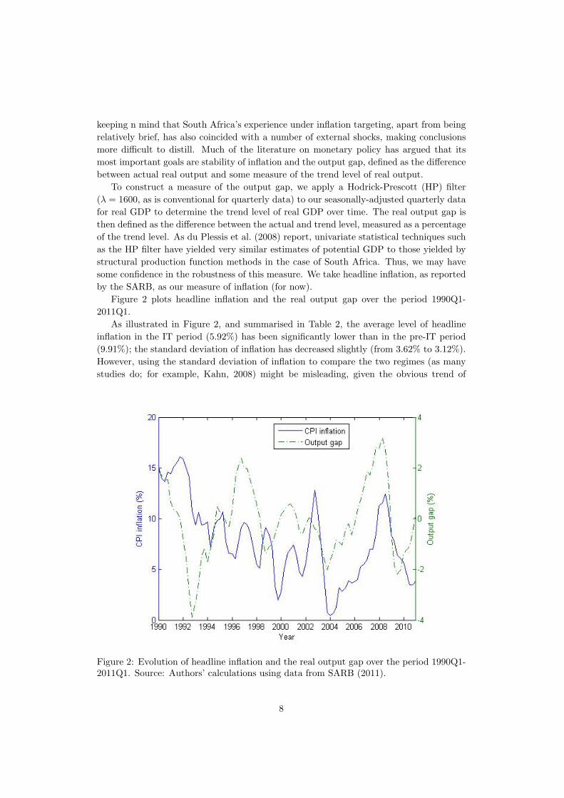
Figure 2 plots headline inflation and the real output gap over the period 1990Q1-

2011Q1.

As illustrated in Figure 2, and summarised in Table 2, the average level of headline

inflation in the IT period (5.92%) has been significantly lower than in the pre-IT period

(9.91%); the standard deviation of inflation has decreased slightly (from 3.62% to 3.12%).

However, using the standard deviation of inflation to compare the two regimes (as many

studies do; for example, Kahn, 2008) might be misleading, given the obvious trend of

Figure 2: Evolution of headline inflation and the real output gap over the period 1990Q1-2011Q1. Source: Authors’ calculations using data from SARB (2011).

8

disinflation in the pre-IT period, from around 15% in 1990Q1 to around 2% in 1999Q4.4

To address this, we apply a straight-line trend to each period’s inflation evolution, and

measure the standard error of detrended inflation. This procedure yields a substantially

lower standard deviation (1.86%) for the pre-IT period than for the IT period (3.11%).

The average growth rate of output increased from the pre-IT period (1.40%) to the IT

period (3.57%), while the standard deviation of the output gap decreased slightly from

pre-IT (1.54%) to IT (1.37%). However, the sample period is too short for these results to

be considered telling. In addition, the periods in question saw significant external shocks.

Clearly, if low and stable inflation were the sole factor by which the SARB is judged,

the Bank could not hope for a favourable review. Despite the decrease in the average

headline inflation rate under IT, CPIX inflation exceeded the upper bound of the target

zone (6%) in 14 of the 28 quarters between 2002Q1 (the first year for which the inflation

target was intended to be achieved) and 2008Q4 (the date at which the CPIX target was

discarded). Headline inflation exceeded 6% in 16 of the 37 quarters between 2002Q1 and

2011Q1. The regular achievement of inflation targets is key both in promoting credibility

of an inflation targeting central bank and in stabilising expectations of inflation at or

near the target. That the SARB regularly misses the inflation target casts doubt on how

successful it could have been in achieving these two goals.

5 The instrument reaction model

In this section, we compare the behaviour of the SARB pre- and post-adoption of inflation

targeting by attempting to fit to the instrument-setting of the SARB generalised Taylor-

like rules of the form

it = i∗ + φπ(Etπt+T |t − π∗) + φy(Etyt+τ |t) + θ · zt, (1)

where it is the period-t nominal interest rate, i∗ is the equilibrium nominal interest rate,

Etπt+T |t is the Reserve Bank’s period-t expectation5 of the average inflation rate between

periods t and t+T , π∗ is the target rate of inflation, Etyt+τ |t is the Reserve Bank’s period-t

expectation of the average output gap over the period t to t+ τ , and zt is a vector of other

variables to which the Reserve Bank might respond. φπ, φy and θ are subjective weights,

to be estimated. We use the expectations of future inflation and output since it is to these

variables that monetary policy usually responds, cognisant of the fact that its influence

is not immediate. However, not having knowledge of these expectations, we shall have to

proxy for them using variables we do have at our disposal.

We take as the nominal interest rate the end-of-quarter repo rate. Other studies have

used the treasury bill rate as the measure for the nominal interest rate; since the treasury

4Indeed, if inflation had decreased in a perfectly straight line from its beginning to end levels in thepre-IT period, the standard deviation of inflation would have been 3.94%.

5It is important that the forecast considered is the central bank’s internal forecast, rather than anexternal forecast or market expectation. If the central bank lets its instrument react systematicallyto market expectations, there may be inherent instability, nonuniqueness or nonexistence of equilibria(Bernanke and Woodford, 1997; Svensson, 2000). Using an estimation of a specification like (1) to analysemarket expectations (as Naraidoo and Gupta (2009) do for the case of South Africa) would also bemisleading, since the central bank’s reactions depend on its own expectations.

9

bill rate and the repo rate are almost perfectly correlated (correlation coefficient of 0.975

in our sample), this should have no meaningful effect on our results.

For now we proxy the SARB’s expectations of future inflation and the output gap by

their contemporaneous levels. For now, then, the specification of (1) that we shall consider

is

it = i∗ + φπ(πt − π∗) + φyyt + θ · zt. (2)

This study seeks to estimate such Taylor-like rules in order to analyse the relative

weights the SARB accorded to monetary policy targets when setting interest rates in the

periods under study. Our discussion of the pre-IT period in Section 4.1 suggests that

emphasis was placed on an eclectic set of indicators, so that the Reserve Bank’s behaviour

could not be well approximated by the the basic Taylor Rule. Rather, we might expect

the fit to improve as addional indicators are introduced into the specification.

For the IT period, we expect estimations of the above specification to return a signif-

icant coefficient on the inflation gap, since it is the stability of this variable that is the

overriding objective of monetary policy under inflation targeting. However, there is also

a provision in the SARB’s mandate that allows for consideration of variables other than

inflation; through our estimation of Taylor-like rules we hope to gain insight into what

variables the SARB considers in exercising this flexibility. For example, a significantly

positive coefficient on the output gap would be evidence that the SARB adjusts counter-

cylically with demand shocks but accommodates supply shocks (which are reflected in the

trend level of output).

One difficulty, to be discussed in greater detail below, is that our proxy for expected

inflation, namely current inflation, may be too simple; Svensson (2000) points out that

the inflation forecast of a central bank is likely to depend on a large number of variables.

If we discover these variables to be significant in estimations of Taylor-like rules, their

significance may simply reflect their weighting in the SARB’s inflation forecast, rather

than the SARB’s exercising flexibility by targeting these variables directly. Section 5.8

provides a detailed analysis of this potential problem.

We shall use our data to estimate the coefficients in (2), beginning with the simplest

form (z = 0) and gradually use more complicated specifications. Naturally, the most

robust observations will be those of later models, since omitted variable bias may play a

large role in the estimations of simpler specifications. This is a caveat we shall keep in

mind when discussing the results of earlier specifications.

The econometric estimations will be carried out by OLS, and thus we first consider

whether the time series in question are stationary or not, a subject with which the following

subsection concerns itself. It is also important to note that the explanatory variables in (2)

can not be strictly exogenous, since the nominal interest rate affects future values of the

explanatory variables. However, since we use the end-of-quarter repo rate, the explanatory

variables are contemporaneously exogenous, so that our estimates will be consistent in the

absence of any other econometric problems.

5.1 Stationarity of the variables

Using OLS to estimate an equation in which two or more non-stationary variables lurk may

result in the conventional t and F tests suggesting relationships where none exist. It also

10

may result in an artificially high R-squared. This is the problem of spurious regression,

first identified by Yule (1926).

To test for stationarity, we employ a range of Dickey-Fuller tests; the results are re-

ported in Table 3 in the Appendix. The tests unanimously fail to reject the hypothesis of a

unit root in the repo rate for both the pre-IT and IT periods, as well as the rate of inflation

for the pre-IT period. There is also a strong suspicion of a unit root in the output gap for

the IT period. The results for the other variables are mixed, with some periods showing

evidence of stationarity and others not. These results necessitate a careful consideration

of how we might alter our functional form to deal with the threat of spuriosity.

In response to the strong suspicions of nonstationary variables, we take the first differ-

ence of the equation to be estimated (2), which yields the general specification:

∆it = φπ∆πt + φy∆yt + θ ·∆zt. (3)

It is important to keep in mind that the coefficients in (3) are identical to those in (2),

and thus their interpretation (and that of our estimates of them) is unchanged.

It is interesting to note that the use of first differencing (or indeed, any other method)

to guard against spuriosity in the estimation of Taylor-like rules seems to be the exception

rather than the rule. For example, Clarida et al. (2000), in estimating a general Taylor-like

rule for the United States, assume that both the inflation rate and the nominal interest rate

are stationary, despite finding evidence (via conventional unit root tests) to the contrary.

In defending this assumption, they point to theoretical reasons for believing the time series

to be stationary, as well as the low power of the unit root tests employed.

Among South African studies, Naraidoo and Gupta (2009) claim that unit root tests

confirm that the nominal interest rate, inflation and the output gap are stationary variables

over the period we are considering, though the results are not reported. It is not clear

whether the authors carried out the tests for different periods, a potentially significant

consideration given the fact that our results show evidence of the stationarity of some

variables to alter between the pre-IT and IT periods.6 Rangasamy (2009) also argues

that, in considering the inertia of inflation, one must account for potential structural

breaks. He shows that, in the case of South Africa, conventional Chow tests reject the

hypothesis of no structural change in the inflation process (in an econometric specification

similar to the unit root tests we have employed) at the point 1999Q4. It is thus vital

that unit root tests be carried out for each period when analysing the stationarity of the

variables.

An alternative technique, facing potential nonstationarity in variables, is to test for

cointegration. Engle-Granger tests (Engle and Granger, 1987) were carried out for both

periods, using the critical values provided by MacKinnon (2010); the results are presented

in Table 4. First, we tested for cointegration between it, it−1, πt, yt and et: our results

provide evidence for cointegration in the pre-IT period (significant at the 5% level) but

not in the IT period (not significant at the 10% level). Omitting the output gap measure

(which displays evidence of stationarity, and indeed is constructed as such) and testing for

cointegration between the remaining variables, we again find evidence of cointegration in

6Indeed, changes in the level of inertia of variables are significant not just on econometric grounds, buton analytical grounds as well. For example, one of the commonly-used tests of the success of inflationtargeting is whether inflation has come to exhibit less inertia or not (Ball and Sheridan, 2005).

11

the pre-IT period (5% level) but not in the IT period. That we cannot reject the hypothesis

of non-cointegration for the IT period suggests that we should not rely on cointegration

in our regressions for this period; for the sake of comparability, we do the same for the

pre-IT period as well, and so we shall use OLS on the first-differenced specification for

both periods.

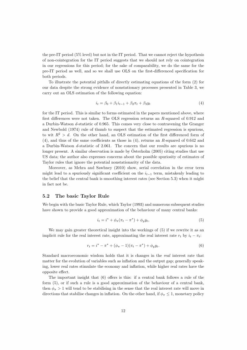
To illustrate the potential pitfalls of directly estimating equations of the form (2) for

our data despite the strong evidence of nonstationary processes presented in Table 3, we

carry out an OLS estimation of the following equation:

it = β0 + β1it−1 + β2πt + β3yt (4)

for the IT period. This is similar to forms estimated in the papers mentioned above, where

first differences were not taken. The OLS regression returns an R-squared of 0.912 and

a Durbin-Watson d-statistic of 0.965. This comes very close to contravening the Granger

and Newbold (1974) rule of thumb to suspect that the estimated regression is spurious,

to wit R2 > d. On the other hand, an OLS estimation of the first differenced form of

(4), and thus of the same coefficients as those in (4), returns an R-squared of 0.642 and

a Durbin-Watson d-statistic of 2.061. The concern that our results are spurious is no

longer present. A similar observation is made by Osterholm (2005) citing studies that use

US data; the author also expresses concerns about the possible spuriosity of estimates of

Taylor rules that ignore the potential nonstationarity of the data.

Moreover, as Mehra and Sawhney (2010) show, serial correlation in the error term

might lead to a spuriously significant coefficient on the it−1 term, mistakenly leading to

the belief that the central bank is smoothing interest rates (see Section 5.3) when it might

in fact not be.

5.2 The basic Taylor Rule

We begin with the basic Taylor Rule, which Taylor (1993) and numerous subsequent studies

have shown to provide a good approximation of the behaviour of many central banks:

it = i∗ + φπ(πt − π∗) + φyyt, (5)

We may gain greater theoretical insight into the workings of (5) if we rewrite it as an

implicit rule for the real interest rate, approximating the real interest rate rt by it − πt:

rt = i∗ − π∗ + (φπ − 1)(πt − π∗) + φyyt. (6)

Standard macroeconomic wisdom holds that it is changes in the real interest rate that

matter for the evolution of variables such as inflation and the output gap; generally speak-

ing, lower real rates stimulate the economy and inflation, while higher real rates have the

opposite effect.

The important insight that (6) offers is this: if a central bank follows a rule of the

form (5), or if such a rule is a good approximation of the behaviour of a central bank,

then φπ > 1 will tend to be stabilising in the sense that the real interest rate will move in

directions that stabilise changes in inflation. On the other hand, if φπ ≤ 1, monetary policy

12

will tend to be destabilising by accommodating changes in inflation. A similar distinction

can be made between stabilising and destabilising policy if φy is greater than or less than

zero respectively (Clarida et al., 2000). This stability benchmark (φπ > 1, φy > 0), known

as the ‘Taylor principle’, is generalisable to any of the linear Taylor-like rules of the general

form (1).

We now estimate the coefficients in (5), first differencing and including a zero-mean

white noise term to yield:

∆it = φπ∆πt + φy∆yt + νt. (7)

The pre-IT regression, regression (i) in Table 5, yields an estimate for the coefficient

on the inflation gap of φπ = 0.322, statistically significant at the 5% level. The coefficient

on the output gap is statistically indistinguishable from zero at conventional levels. As

expected, the current specification provides a poor fit for the pre-IT period, with an R-

squared of just 0.127.

The regression for the IT period, regression (ii) in Table 5, returns estimates of φπ =

0.302 and φy = 0.574, both statistically significant at the 1% level. The estimated equation

provides a far better fit than for the pre-IT period, with an R-squared of 0.599.

A number of tentative observations may be drawn from these results. First, as expected,

the simple Taylor-rule provides a poor approximation of the instrument reaction behaviour

of the SARB pre-IT (and a good fit for the IT period). Still, as we consider more eclectic

forms of (2), the fit of the pre-IT regressions will not match the fit of the simple Taylor

Rule in the IT period, suggesting that monetary policy has become both more rules-based

with the adoption of IT (or more precisely, that instrument reactions have more closely

approximated a rule under IT), as well as simpler.

Second, that the SARB’s IT regime is flexible is evidenced by the significantly positive

coefficient on the output gap for the IT period - the SARB responds significantly to short

term movements in the output gap. This counters claims by COSATU and others that

the Reserve Bank focusses too strictly on inflation, and gives little or no consideration to

the output gap.

Third, in both periods the coefficient on the inflation gap is significantly smaller than

unity, a disturbing result given our discussion of the Taylor principle above. This charge,

that monetary policy in both periods was conducive to an unstable inflation process, is a

serious one, and will be discussed further below (drawing on the results of more predictor-

laden models, with which the problem of omitted variable bias is lessof a concern).

Fourth, it would be reasonable to expect φπ to have increased under IT; the results

tentatively suggest that this might not be the case. Of course, this may be an artifact of

omitted variable bias, although the finding will persist in later regressions as well. This

counterintuitive observation is one that casts some doubt on the SARB’s commitment to

a greater focus on price stability under inflation targeting.

5.3 Accounting for interest rate smoothing

Our specification may be modified slightly to account for the oft-noted tendency of central

banks to smooth changes in interest rates; i.e. to change interest rates to the desired

level gradually, rather than immediately. To account for this, we employ the following

specification for the current nominal interest rate in terms of the target rate and the

13

previous period’s rate:

it = αit−1 + (1− α)it, (8)

where it is the target nominal interest rate given by (2). The central bank, cognisant

of its target level for the interest rate, adjusts the actual interest rate a positive fraction

1− α ∈ (0, 1] of the gap between the previous period’s actual rate and the target rate.

The parameter α is thus a measure of the degree of interest rate smoothing exercised by

the central bank. To illustrate, if the target rate were to change to i in period t, and

remain constant thereafter, we have the following expression for the period t+n difference

between the actual and target interest rates:

it+n − i = αn[

it − i]

.

The larger is α, the slower the interest rate adjusts towards the target level.

Incorporating (8) into our general specification yields

it = αit−1 + (1− α) [i∗ + φπ(πt − π∗) + φyyt + θ · zt] . (9)

This specification permits an interpretation of the coefficients in terms of the ‘short run’

and the ‘long run’: The immediate response to a unit change in, say, the inflation gap is

to change the interest rate by (1 − α)φπ. This may be seen as the short run reaction. If

the target interest rate remains unchanged thereafter, the eventual (asymptotic) effect is

that the interest rate changes by φπ. This is the long run effect; it is necessarily greater

in magnitude than the short run effect. The same holds for the coefficients on the output

gap and other predictors.

Our first estimates of (9) will be of the simple case where zt = 0, i.e. of the basic Taylor

Rule augmented to account for interest rate smoothing. First differencing and including a

zero-mean white noise term results in the following specification

∆it = α∆it−1 + (1− α)φπ∆πt + (1− α)φy∆yt + νt, (10)

which we estimate using OLS; the results are displayed in columns (iii) and (iv) of Table

5. We report the coefficients on the predictors (estimates of (1− α)φπ etc., the short run

reaction parameters), as well as the implied values of the long run parameters φπ and φy,

calculated in each case using the respective point estimate of α, with the standard errors

calculated using the delta method.

For the pre-IT period, the estimate for α, the interest rate smoothing parameter, is

statistically indistinguishable from zero; there is no evidence at this stage that the Reserve

Bank smoothed interest rates in a systematic way in the pre-IT period. The coefficients on

the inflation and output gaps are also statistically insignificant, and the model provides a

poor fit, with an R-squared of just 0.150. Our estimates of the long run inflation reaction

parameter φπ is positive (0.299) and statistically significant at the 10% level, while that

of φy is statistically indistinguishable from zero.

The estimated interest smoothing parameter for the IT period is 0.252; it is significant

at the 5% level. Thus, we find initial evidence of systematic interest rate smoothing under

IT. The coefficients on the inflation and output gaps are both significant at the 1% level,

and our accounting for interest rate smoothing has slightly improved the fit of the model,

14

with the R-squared having increased to 0.642.

Using our point estimate of α, we obtain the following estimates for the IT period:

φπ = 0.292 and φy = 0.762, both significant at the 1% level. The estimates of the Reserve

Bank’s weights on the inflation gap for the two periods have not changed substantially

after accounting for interest rate smoothing, and are still substantially (and statistically

significantly) below unity, in contravention of the Taylor principle. Our estimate of the

coefficient on the output gap has increased for the IT period, and is still statistically

significantly positive, providing further evidence that the SARB’s IT regime is flexible.

5.4 The real exchange rate

5.4.1 Should the real exchange rate be targeted?

One of the major criticisms levelled at South Africa’s inflation targeting regime, most

prominently by COSATU, is that it exerts little control over the exchange rate; South

Africa’s real exchange rate is extremely volatile compared to most other countries. A

volatile exchange rate, or one that is persistently overvalued, can have negative repercus-

sions for international trade and investment, and so, some say, the SARB should focus

more on the exchange rate.

It should be made clear from the outset is that an inflation targeting regime does

not ignore the exchange rate. Since a depreciation in the exchange rate tends to place

upward pressure on inflation, while an appreciation has the opposite effect, a regime that

is concerned (even solely) with inflation would respond to movements in the exchange rate,

and tend to do so in the direction that stabilises the exchange rate as well (by increasing

the interest rate in response to a depreciation, and vice versa).

If exchange rate stability is an objective of monetary policy, there are a number of

strategies to achieve this end.

The most extreme form of exvhange rate targeting would be some form of fixing the

exchange rate, the major attractions of which are a simple nominal anchor and a si-

multaneous reduction in the currency risk component in domestic interest rates. The

major detraction is that domestic interest rates must be aligned to those in the anchor

country/countries - monetary policy forfeits the ability to respond directly to domestic

shocks. Since South Africa’s economy is not highly integrated with any of the more stable

economies of the world, pegging the rand to any of their currencies would result in our

suffering their economic shocks, while being unable to adequately address our own. More-

over, the mobility and size of modern capital markets have made defending fixed exchange

rates against speculation enormously expensive; this is the practical consideration Obst-

feld and Rogoff (1995) have in mind when they emphatically proclaim that ‘it is folly to

try to recapture the lost innocence of fixed exchange rates’. The case for target bands is

not much stronger - when the band’s boundary is reached, the problems of fixed exchange

rates become relevant.

A less severe strategy is for the monetary authority to respond to movements in the real

exchange rate using the instruments available to it, (at least partly) independent of any

effect the change in the exchange rate might have on other variables such as inflation; i.e.

to directly stabilise the real exchange rate via its instrument reaction. Beyond responding

to exchange rate movements only insofar as they signal changes in inflation (though this

15

would be, as noted, exchange rate-stabilising to some extent), trade-offs between the goals

of monetary policy would necessarily emerge - required interest rate movements to stabilise

inflation, the exchange rate, and the output gap are not always harmonious. In this sense,

the interest rate is a ’sledgehammer’, not a ’surgical scalpel’: it cannot be employed to

affect one variable (the exchange rate, say) without affecting a number of other variables

as well (inflation, output, etc.).

A good example of this ‘sledgehammer’ effect is found in the savage interest rate spike

with which the SARB reacted to the 1997/8 currency depreciation. While the rand did

strengthen slightly, the country also suffered a plunge in the real output gap. Aron and

Muellbauer (2007) compare this reaction to the more moderate one with which the SARB

responded to the 2001 rand depreciation; the latter saw a lower cost to output and a

greater degree of stability overall.

5.4.2 Has the real exchange rate been targeted?

To test whether the real exchange rate formed part of the decision making of the SARB pre-

and post-adoption of IT, we add a measure of the real exchange rate to our specification

by incorporating it as an element of zt. Because we would like to make some fairly robust

observations at this stage, we include measures of asset prices (see next section) to mitigate

the possibility of omitted variable bias. We keep the specification that accounts for interest

rate smoothing, so that the equation to be estimated is

it = αit−1 + (1− α) [i∗ + φπ(πt − π∗) + φyyt + φe(et − e∗) + θ · zt] , (11)

where et is the real exchange rate7 and e∗ is the target real rate. zt includes the asset

price gaps that will be defined properly in the next section. In keeping with the nature of

the other variables in the specification, we interpret et − e∗ as a ‘gap’ or deviation from

equilibrium, in percentage form.8 We first-difference (11) and estimate the coefficients

using OLS, as before. The results for the two periods form columns (v) and (vi) in Table

5 in the appendix.

Adding the real exchange rate gap (and the asset price gaps) to the pre-IT regression

substantially improves the fit of the model, with the R-squared increasing to 0.388 (from

just 0.150).9 This confirms the ‘eclectic’ nature of monetary policy pre-IT: variables other

than those specified in the basic Taylor Rule explain more of the instrument variability

than the ‘classic’ variables (inflation and the output gap). The coefficient on the real

exchange rate is negative (−0.135), and significant at the 1% level, suggesting that the

SARB tended to raise rates in response to depreciations and to lower rates in response to

appreciations, behaviour consistent with attempting to stabilise the exchange rate. The

coefficient on the inflation gap is significant at the 10% level, while the coefficient on the

output gap is insignificant. The coefficient on the inflation gap, when augmented by the

7We use the real effective exchange rate calculated by the IMF, which is defined as an index with baseof 100. The rate is defined in local currency per unit of foreign currency, so that an increase correspondsto an appreciation.

8We take the target or equilibrium value of e as 100, so that deviations from the target are percentagesof the target as well. If the equilibrium exchange rate is not 100, but some other constant, the only effecton our estimation will be a scaling of φe - its sign and significance will be unchanged.

9Adding the real exchange rate to the specification, but not the asset price gaps, results in a still muchimproved R-squared of 0.256.

16

factor 1/(1− α), is still significantly below unity. There is still no evidence of systematic

interest rate smoothing in the pre-IT period, with the coefficient on the lagged repo rate

insignificant, even at the 10% level.

The inclusion of the exchange rate and asset price gaps for the IT period only marginally

improves the fit of the model, with the R-squared increasing to 0.680. The coefficient on

the real exchange rate for the IT period is negative, and statistically significant at the

10% level, though it is small in magnitude (−0.030, compared to the pre-IT estimate

−0.135), suggesting that, in terms of instrument decisions, the SARB has not responded

substantially to changes in the real exchange rate. Again, there is evidence of interest rate

smoothing, with the coefficient on the lagged repo rate significant at the 5% level, and

similar in magnitude to that in the previous IT regression. The coefficients on the inflation

and output gaps have not changed noticeably with the inclusion of the real exchange rate

and asset price gaps, with the estimates of both the short-run and long-run inflation

reaction parameters still significantly below unity for the IT period.

5.5 Asset prices

5.5.1 Should asset prices be targeted?

The recent financial crisis has raised questions around the extent to which monetary policy

should react to movements in asset prices;10 inflation targeting in particular has been

accused of ignoring asset price bubbles.

Again, we note that inflation targeting does already respond to asset price movements

insofar as they signal changes in expected inflation. Since asset prices, aggregate demand

and inflation expectations tend to move in the same direction, interest rate responses under

an inflation targeting framework will tend to induce the correct (directionally) stabilisation

response with respect to each in the face of asset price instability. Moreover, because

asset price shocks fall primarily on the demand side of the economy, standard business

cycle theory suggests that inflation targeting is a particularly good policy to play this

countercyclical role (Sørensen and Whitta-Jacobsen, 2005, chap. 20). Price stability and

financial stability can be complementary objectives, and inflation targeting provides a

unified framework to address both. Furthermore, public knowledge that a credible central

bank systematically addresses asset price movements countercyclically under an inflation

targeting framework can help to reduce the ‘irrational exuberance’ that leads to bubbles

in the first place.

Critics of inflation targeting contend that the monetary authorities should provide

responses to asset price movements over and above those dealing with inflationary expec-

tations. In other words, central banks should target asset prices to some degree. The

difficulty with such a strategy is that it is nearly impossible to tell whether movements in

asset prices are the result of fundamental factors or nonfundamental factors.11 As Mishkin

(2007) notes, to assume that monetary authorities can distinguish between fundamental

10We do not consider exchange rates here, although they are asset prices, since they have been separatelyconsidered in a previous section.

11Or indeed, both. If it were not already difficult enough to distinguish between fundamental andnonfundamental movements, it would be even more difficult to accurately quantify the two if asset pricemovements were the result of both. A correctly tailored response under an asset price targeting frameworkwould then be practically impossible.

17

and non-fundamental movements is to assume that they have better information and pre-

dictive ability than the private sector. This is not to deny the existence or damaging effects

of asset price bubbles - the point is that, without an informational advantage over private

markets, monetary authorities would be as likely to mispredict the presence or absence

of a bubble as private markets, and as a result would frequently be mistaken, damaging

their credibility. A unified strategy of inflation targeting, on the other hand, allows the

central bank to respond to asset booms and busts without getting into the murky business

of deciding what is fundamental and what is not (Bernanke and Gertler, 2000).

Moreover, the ‘sledgehammer’ effect of interest rates is even more problematic with

asset prices; their sensitivity to interest rate changes is generally much lower than that of

output, inflation or the exchange rate. For example, the interest rate increase needed to

deflate a supposed bubble is likely to wreak havoc on the rest of the economy.

Our contention is that monetary policy responses to asset price movements should

be limited to addressing the inflationary repercussions of those movements - asset price

regulation may fall more appropriately under financial market regulation and supervision

than monetary policy control.For example, if rapidly rising prices in the housing market are

deemed to be unsustainable, there are more effective instruments to deflate the supposed

bubble than monetary policy, including regulation of loan-to-value ratios and minimum

mortgages (Svensson, 2010).

5.5.2 Have asset prices been targeted?

Some studies that seek to estimate an instrument reaction function for the SARB have

incorporated asset prices by adding a composite asset price index to Taylor-like specifica-

tions (see, for example, Naraidoo and Paya, 2010). We find the use of a composite asset

price index inadvisable, since it imposes a given weighting for each asset price within the

index and thus within the rule as a whole. A less restrictive method for testing would be

to include asset prices individually, and to test the hypothesis of their joint significance;

this is the method we employ.

In testing whether the instrument reaction decisions of the Reserve Bank have depended

on asset prices in the two periods under study, we consider two asset prices distinct from

the exchange rate: share prices (we use the All Share Index) and house prices (ABSA’s

Average House Price Index). We add to our specification two measures: a share price

gap and a house price gap, both calculated using a Hodrick-Prescott filter (λ = 1600) and

taken as percentages of the trend. We use this measure rather than, say, year-on-year

percentage increases, to account for the fact that these variables often have distinct trends

that cannot be captured adequately and systematically by taking percentage increases and

the like.12 Our specification is then:

it = αit−1 + (1− α) [i∗ + φπ(πt − π∗) + φyyt + φeet +Φ ·At] , (12)

where At is the vector of asset price gaps (sharegapt, housegapt), and Φ = (Φsh,Φh) is

12In particular, taking percentage increases and incorporating them into our linear specification implic-itly assumes that the target level for the percentage increases is constant, and that for the prices themselvesis exponential. One can readily see from diagrams of the evolution of these asset prices that this wouldbe a poor approximation of any acceptable trend.

18

the vector of the weights placed on the asset price gaps.

(12) is the fully defined version of (11), whose coefficients we have already estimated,

with the results presented in columns (v) and (vi) of Table 5.

For the pre-IT period, of the asset price gaps, only the coefficient on the share price gap

is statistically significant at conventional levels, being significant at the 5% level. The sign

of the coefficient on the share gap is positive, in line with what we would expect. Adding

the asset price gaps to a specification that already includes the exchange rate increases

the R-squared from 0.256 to 0.388, suggesting that asset prices explain a large part of

the SARB’s instrument decision variation pre-IT. This is confirmed by an F -test of the

hypothesis that the asset price gaps are jointly insignificant pre-IT: the null hypothesis of

no significance is rejected at the 5% level (F2,33 = 3.55; p = 4.00%).

None of the coefficients on the asset gaps is significant at conventional levels for the

IT period. The R-squared increases only marginally when we add the asset price gaps to

a regression that already includes the real exchange rate, from 0.677 to 0.688; an F -test

fails to reject the hypothesis that the asset prices are jointly insignificant at conventional

levels (F3,38 = 0.63; p = 53.65%). The evidence suggests that, under inflation targeting,

the SARB has not targeted asset prices.

5.6 What measure of inflation?

The question of what measure of inflation should be targeted is equivalent to the question

of what prices the monetary authority considers important to stabilise the growth of in

the medium term. Since the central bank does not know, but can only forecast, what the

medium-term level of that inflation rate will be, another question is raised: What current

measure of inflation, in conjunction with other variables, is most useful in indicating what

the medium term level of the targeted inflation rate will be? It may seem obvious that

the current level of the variable whose medium term level is targeted would best perform

this role, but we shall argue below that this is not necessarily the case.

With regard to the first question, viz. what variable should form the medium term

target, we consider four measures of inflation relevant to South Africa: headline (CPI)

inflation, CPIX inflation, domestic inflation, and core inflation. Roughly speaking, CPI

inflation is the rate of change of the price of a bundle of goods that is representative of the

typical consumption patterns of a South African citizen. This bundle includes imported

goods, so that CPI inflation depends on the domestic price of goods produced elsewhere.

As noted previously, CPIX inflation is the rate of change of the price of the same bundle

used in calculating CPI inflation, but excluding the mortgage interest cost. Domestic price

inflation is the rate of change of the price of a bundle of goods produced domestically.

Finally, core inflation is calculated in the same way as CPI inflation, but excludes the

prices of certain food products, the cost of mortgage bonds and certain indirect taxes.

The SARB initially chose CPIX inflation over CPI inflation as the variable to target,

since the mortgage interest payments that form part of the CPI measure (but not CPIX)

are directly affected by changes in the repo rate, resulting in an unwanted feedback from

inflation to changes in the repo rate back to inflation. However, this disadvantage of CPI

inflation targeting can be, and has been in most countries that target CPI inflation, elimi-

nated by altering the method with which housing costs are calculated. At the beginning of

19

2009, the Reserve Bank changed its target variable to CPI inflation, altering the measure-

ment of housing costs from mortgage interest costs to a rental equivalence measure (Kahn,

2008). Thus, in practice, CPI inflation targeting and CPIX inflation targeting collapse to

a single case, which we shall call CPI inflation targeting. This allows us to simplify our

discussion to CPI inflation targeting, domestic price inflation targeting and core inflation

targeting.

CPI inflation targeting has the benefit that it targets a measure of inflation that applies

to the typical consumption patterns of a South African citizen; i.e. it targets the most

meaningful measure of inflation for most members of society. In addition, it is easily

understood by the public. The problem with targeting CPI inflation is that the measure

is influenced by goods whose prices are very volatile (such as food). This leads to a

larger degree of uncertainty in forecasts of future inflation (and thus greater uncertainty

in instrument setting), and adds an unavoidable element of volatility to a variable whose

stability is the expressed aim of monetary policy. Moreover, by using such a broad measure

of inflation, the Bank’s target may be affected by exogenous shocks over which it has no

control (van der Merwe, 2004).

Domestic price inflation targeting excludes the price of imported goods from the target.

To the extent that imported goods form a significant part of the consumption preferences

of a typical South African, this measure does not capture a meaningful (from society’s

perspective) measure of inflation. Domestic price inflation is also influenced by goods

whose prices are volatile, leading to the same problems as with CPI inflation targeting

noted above. These represent significant weaknesses, which have led all inflation-targeting

countries to eschew domestic price inflation targeting.

Core inflation targeting removes the effects of food prices and other volatile prices from

the target. Again, to the extent that these goods form a significant part of the typical

South African’s consumption bundle, the target will not be meaningful from society’s per-

spective. It is also more difficult for the public to understand than CPI inflation targeting,

potentially damaging credibility (van der Merwe, 2004). However, using core inflation as

the target would provide the advantage that the volatile prices that are problematic for

CPI inflation targeting would not be part of the target, allowing the central bank to avoid

the problems that these volatile prices cause for CPI inflation targeting.

It is notable that the core index in South Africa, unlike most countries’ core indexes,

includes a nontrivial weighting for an index of the petrol price (currently 3.99%, higher

than its weighting in the CPI). Thus, using the official measure of core inflation as the

target would remove some, but not all of the volatile prices over which monetary policy

has no control from the targeted measure.13

The problems inherent in domestic price inflation targeting warrant its exclusion from

further consideration as a viable target. In choosing between CPI inflation and core

inflation, a tradeoff has been identified between the meaningfulness and understandability

13Of course, this difficulty could easily be overcome by removing the petrol price from the core index.It truly is odd that it is included in the core measure, since the definition of ‘core inflation’ essentiallyprohibits its inclusion. It is even more bizarre that petrol’s weighting in the core index is even higherthan petrol’s weighting in the CPI. Core inflation certainly should account for some of the second roundeffects of changes in the oil price, but directly including the oil price in the measure results in even verytemporary changes in the oil price (which should have only limited pass through under a credible regime)causing fluctuations in the official measure of core inflation.

20

of the target on one hand (a benefit of CPI inflation targeting, and a weakness of core

inflation targeting), and the potentially misleading effects of volatile prices and those over

which the monetary authority have no influence on the other hand (a problem with CPI

inflation targeting, but not for core inflation targeting). In reality, a flexible regime with a

medium-term horizon for its target can have, to a certain extent, the best of both worlds.

It can use CPI inflation as its target, and thus enjoy the benefits of a meaningful and

publicly understandable target, but can choose to ignore temporary changes in prices that

are inherently volatile or over which the monetary authority has no control, since its target

is neither immediate nor strict. Of course, policy decisions that are based on a large degree

of discretion must be communicated extensively to the public to maintain credibility.

Whatever the measure of inflation used, though, the target is a future one, often as

far as two years in the future. This raises the question of which current measure provides

the most use in foreasting the level of the target inflation rate in the future. The problem

with using current CPI inflation to forecast future inflation, even if the target is future

CPI inflation, is immediately obvious: because CPI inflation is influenced by goods whose

price is inherently volatile, the current level of CPI inflation comprises a trend component

of prices that are not volatile, and a more variable component of prices that are volatile

and whose current level is thus very much temporary. The latter component is useless in

forecasting what inflation will be in the future, and if current CPI inflation is blindly used

to this end, it could be very misleading.

Core inflation, on the other hand, does not (or at least, should not) include these volatile

prices. Thus, it provides a better indicator of the underlying trend of inflation, and in this

regard is more useful in forecasting future inflation than CPI inflation is (Blinder and Reis,

2005). Also, because most of the prices that make up the core index are not reset very

often, they are necessarily set with future inflation in mind (Krugman, 2010).

We might therefore expect core inflation to be more significant in the Reserve Bank’s

forecast model for future headline inflation, and to the extent that the Bank’s instrument

reaction decisions are well approximated by a forward-looking rule of the general form

specified in (1), we would expect core inflation to be more significant (and possibly to

have a higher coefficient as well) in estimations of rules of the form (1).

To test these hypotheses, we include each of CPI inflation, CPIX inflation and the

official measure of core inflation in a separate regression of the form specified in (11).

Since the official measurement of CPI was altered at the end of 2008, we estimate the

specifications for the period 2000Q1-2008Q4, so that our results are comparable. Again,

in each case we first-difference and estimate the coefficients using OLS. The results form

columns (vii), (viii) and (ix) of Table 5.

The CPI inflation and CPIX inflation specifications provide similarly good fits: the CPI

specification has an R-squared of 0.659, while the R-squared for the CPIX specification

is 0.658. Both measures of inflation are significant at the 5% level in their respective

regressions, with the coefficient on CPIX inflation higher than that on CPI inflation.

The coefficient on the lagged repo rate is insignificant in the CPI inflation regression,

but is significant in the CPIX inflation regression. Using the point estimates of α in

each regression, the implied estimates of φπ are 0.265 and 0.417 in the CPI and CPIX

regressions respectively, both substantially and statistically significantly below unity.

The core inflation specification provides the worst fit of the three inflation measures,

21

with an R-squared of 0.614; indeed, the coefficient on core inflation is not statistically

distinguishable from zero at conventional levels. Removing the petrol price component

from the official core index (the petrol index’s weight in the core index was 5.44% over

the period 2000-2008) yields a purer core index, which we enter into our specification and

estimate (results not reported in Table 5). The fit improves marginally from the official

core specification, with the R-squared increasing to 0.632, and the core inflation variable

becomes significant at the 10% level (p = 6.1%).

The discussion above, advocating a greater weight on current core inflation since it

should be a better predictor of future inflation, suggests that these should be considered

worrying results. There is no evidence to suggest that the SARB implicitly responded to

changes in core inflation, despite core inflation having a large degree of inertia and thus

providing a better measure of the trend of inflation.

5.7 Discussion of results and their limitations

Our specification now provides a reasonable enough fit for both periods for us to make

some more confident observations. First, as expected, the simpler specifications provide

a poor fit for the pre-IT period, when monetary policy was known to be eclectic. Only

whenwe control for the real exchange rate and some other asset prices does the fit of

the model improve significantly, with both the real exchange rate and the other asset

prices significant at conventional levels. The output gap is insignificant in all of the pre-IT

regressions, suggesting that monetary policy paid little or no attention to output, focussing

rather on other target variables.

For the IT period, the basic Taylor Rule provides a good fit, and even more so when

we augment it to account for interest rate smoothing. The coefficient on the output gap is

significantly positive, suggesting that the inflation targeting regime followed by the SARB

has indeed been flexible. As previously noted, a positive coefficient on the output gap

is also evidence that the Reserve Bank has tended to react countercyclically to demand

shocks but has tended to accommodate supply shocks. In the IT regressions, the coefficient

on the real exchange rate is weakly statistically significant but small in magnitude, while

those on asset prices are not significant, suggesting that monetary policy has paid little

attention to these variables under inflation targeting. CPI and CPIX inflation provide

similarly good fits, while the fit of the specification using core inflation is relatively worse,

despite core inflation’s tendency to be a better predictor of future headline inflation.

The differences between the regimes are thus fairly clear. Broadly, the pre-IT regime

focussed on exchange rates and possibly asset prices, and not on output. The IT regime

has focussed strongly on output, but not on exchange rates and asset prices. The SARB

focussed on inflation in both periods, and its instrument setting behaviour seems to have

been influenced by a tendency to systematically smooth interest rates in both periods.

The major concern raised throughout our analysis has been that the weight on the

inflation gap is low in both periods. (It is also noteworthy that the weight on the inflation

gap seems paradoxically to have decreased under inflation targeting.) A weight on the

inflation gap lower than unity has been shown to result in an unstable inflation process in

a wide range of macroeconomic models; in all of our regressions (both pre-IT and IT), the

short run and (inplied) long run weights on the inflation gap are substantially and statisti-

22

cally significantly lower than unity. This would appear to contravene the Taylor principle

that these weights should be greater than unity, and suggests that the monetary policy of

the SARB has been conducive to inflation instability in both periods, perversely allowing

the real interest rate to rise in response to decreases in inflation, and vice versa. This result

warrants more investigation; in particular, it necessitates a discussion of whether our low

estimates of the inflation weights might be driven by specification or other econometric

issues, rather than a truly low inflation emphasis.

A plausible explanation lies in the relation between the original forward-looking speci-

fication (1) and its contemporaneous counterpart (2), which was the specification we used

in our estimations. The Taylor principle, applied to (1), advises that the coefficient on the

expected future inflation gap be larger than unity. We noted that our proxy for expected

future inflation, viz. current inflation, was likely an oversimplification, since the Reserve

Bank considers many more variables than current inflation in forming its expectation of fu-

ture inflation. The small coefficient on current inflation in our regressions might therefore

reflect the small weight placed on this variable in the SARB’s formation of its expectation

of future inflation, rather than a low weight placed on expected future inflation in the

first place. To illustrate, suppose the SARB’s forecast model for future inflation is of the

simple linear form

Etπt+T |t = γ0 + γ1πt + γ2yt + γ3et +ψ · xt, (13)

where the γi and the elements of ψ are constants, and xt is a vector of other variables the

SARB might consider in forecasting future inflation. Keeping the proxy for the SARB’s

forecast of the future output gap as the output gap’s contemporaneous level, and substi-

tuting (13) into (1), yields a reaction function of the same general form as (2):

it = k + γ1φππt + (γ2φπ + φy)yt + (γ3φπ + φe)et + . . . (14)

where k is a constant. Note that the coefficient on the inflation gap is the product of two

coefficients: the coefficient on expected future inflation in the Taylor-like rule, and the

weight on current inflation in the forecast model for future inflation. If φπ is greater than

unity, in line with the Taylor principle, but smaller than 1/γ1, then the overall coefficient

on the inflation gap will be less than unity, and would be expected to be estimated as such

in an unbiased regression. For example, our point estimate of φπ in the IT regression (vi)

is 0.237. If the true φπ > 1, and any attenuation of our estimate of φπ stems solely from

the above problem, it would be required that γ1 < 0.237.

In fact, (14) highlights a general difficulty in interpreting the results of our regression:

Is the significance of a coefficient on a variable the result of the SARB’s targeting that

variable separately, or is it a result of that variable forming part of the SARB’s forecast of

future inflation? On this question, our regressions are necessarily ambiguous. One point

that can be made is that the two terms in each coefficient on the non-inflation variables

are unlikely to cancel each other out; they should be of the same sign.

Our low estimates of the SARB’s inflation weights could also be the result of attenuation

bias stemming from our inflation variable being mismeasured. Since we are attempting to

characterise the behaviour of the Reserve Bank, it would be most advisable to use real-

time data rather than revised ex-post data, since it is obviously real-time data that the

Reserve Bank uses in its decision-making (Orphanides, 2001). To the extent that revised

23

data is a mismeasured form of real-time data, there is a possibility of attenuation bias

in our estimate of the weights on inflation. If the real-time inflation rate and its revised

ex-post form are related by

πrt = πep + ν,

and the classical measurement error acondition, E(ν|πep) = 0, holds, then we would

expect our estimate of the weight on inflation to be biased towards zero if we use πep in

our regression, rather than πrt.

These caveats notwithstanding, there remain strong reasons to believe that our results

represent evidence that the SARB has been ‘soft on inflation’. First, the estimated co-

efficient on the inflation gap is lower for the IT period than for the pre-IT period. It is

unlikely that structural changes (for example, in the formation of inflation forecasts) can

account for this paradoxical change in apparent emphasis. Second, similar studies (using

current inflation and OLS, and as such, subject to the same general objections as those

raised above) carried out for other countries have yielded estimates of inflation weights

that are significantly above unity.

6 Conclusions

Under inflation targeting, the SARB has missed its official inflation target in 19 of the 37

quarters since the year for which the target was first set. While this gives the lie to the

accusations of COSATU and others that the Reserve Bank focusses too much on meeting

its inflation targets, it also raises serious doubts around how successful the regime has been

with respect to its primary goal, price stability. Indeed, the volatility of inflation seems

to have increased under inflation targeting, relative to the previous monetary targeting

regime. This contrasts with most international experiences of inflation targeting; the

regime has in general been associated with a greater degree of macroeconomic stability.

In this paper, we have sought to explain these anomalies by empirically analysing the

behaviour of the SARB before and after the adoption of inflation targeting, making use

of Taylor-like rules to gain insight into what variables the SARB focussed on (and with

what weightings) when setting its interest rates in the two periods.

Our approximation of an instrument rule for the pre-IT period suggested that the

SARB reacted primarily to changes in inflation, the real exchange rate and other asset

prices in this period; we found no evidence of a tendency to smooth interest rates. The

emphasis on the real exchange rate and other asset prices is consistent with the eclectic

focus this regime is known to have had.

In contrast, our approximation of a rule for the IT period revealed that the SARB

has reacted to changes in inflation and the output gap under inflation targeting, and has

exhibited little or no targeting of the exchange rate or other asset prices. The significance

of the output gap in our IT regressions, along with its relatively large weight, points to

a large degree of flexibility exercised by the SARB (in contrast to COSATU’s claims).

Evidence of a tendency to smooth interest rates in this period was found.

Of major concern is the very low coefficient on inflation in our regressions for both

periods. Theory suggests that a weighting lower than unity for inflation in an instrument

rule could lead to an unstable inflation process, and in every regression our estimate of this

24

weight was both substantially and statistically significantly smaller than this threshold.

This is a particularly disturbing result for the IT period (for which the estimated weighting

was actually lower than that for the pre-IT period), and casts further doubt on the SARB’s

insistence that price stability is its overriding objective.

This low coefficient could be explained away if the SARB places a low weight on current

inflation in its forecast for future inflation, since it is actually the forecast for which it has a

target. The low coefficient on current inflation in our regressions might reflect this, rather

than a weak focus on keeping inflation within the target band. Also, because instrument

decisions in the period under study would have been made making use of real-time data,

while we use ex-post data in our estimations, our results could suffer from the problems

associated with mismeasured variables, and in particular, attenuation bias.

Still, that the coefficient on inflation in our regressions was smaller for the IT period

than for the pre-IT period, and that in similar estimations for other countries, inflation

coefficients significantly greater than unity have been found, support the suspicion that

the SARB has tended to respond more timidly to changes in inflation than theory suggests

it should have.

Thus, we have found evidence that the SARB places too low a weight on its inflation

target when setting the interest rate, which may explain the high volatility of inflation

observed in the IT period.

References

J. Aron and J. Muellbauer. Estimating Monetary Policy Rules for South Africa. The

Centre for the Study of African Economies Working Paper Series, 2001.

J. Aron and J. Muellbauer. Review of monetary policy in South Africa since 1994. Journal

of African Economies, 16(5):705, 2007.

L. Ball and N. Sheridan. Does inflation-targeting matter? In B. Bernanke and M. Wood-

ford, editors, The inflation-targeting debate, pages 249–276. University of Chicago Press,

2005.

B.S. Bernanke and M. Gertler. Monetary policy and asset price volatility. 2000.

B.S. Bernanke and F.S. Mishkin. Inflation targeting: A new framework for monetary

policy? The Journal of Economic Perspectives, 11(2):97–116, 1997.

B.S. Bernanke and M. Woodford. Inflation forecasts and monetary policy. Journal of

Money, Credit & Banking, 29(4), 1997.

O. Blanchard and J. Galı. Real wages, rigidities and the New Keynesian Model. Journal

of Money, Credit and Banking, 39(1):35–65, 2007.

A.S. Blinder and R. Reis. Understanding the Greenspan Standard. 2005.

R. Clarida, J. Galı, and M. Gertler. Monetary Policy Rules and Macroeconomic Stability:

Evidence and Some Theory. The Quarterly Journal of Economics, 115(1):147–180, 2000.

25

A. Cuevas and S. Topak. Monetary Policy and Relative Price Shocks in South Africa and

Other Inflation Targeters. IMF Working Papers, 2009.

D.A. Dickey and W.A. Fuller. Distribution of the Estimators for Autoregressive Time

Series With a Unit Root. Journal of the American Statistical Association, 74(366):

427–431, 1979.

S. du Plessis, B. Smit, and F. Sturzenegger. Identifying aggregate supply and demand

shocks in South Africa. Journal of African Economies, 17(5):765, 2008.

W. Easterly and S. Fischer. Inflation and the poor. Journal of Money, Credit and Banking,

33(2):160–178, 2001.

R.F. Engle and C.W.J. Granger. Co-integration and error correction: representation,

estimation, and testing. Econometrica: Journal of the Econometric Society, pages 251–

276, 1987.

C. Freedman and D. Laxton. Why inflation targeting? IMF Working Paper, 2009.

P. Gordhan. Letter to Gill Marcus, Re: Clarification of Reserve Bank’s mandate. 2010.

C.W.J. Granger and P. Newbold. Spurious Regressions in Econometrics. Journal of

Econometrics, 2:111–120, 1974.

M. Hyvonen. Inflation convergence across countries. Reserve Bank of Australia Research

Discussion Paper, 2004.

IMF. Inflation targeting and the IMF. IMF Working Paper, 2006.

B. Kahn. Challenges of inflation targeting for emerging-market economies: the South

African case. 2008.

P.R. Krugman. The Conscience of a Liberal - Core Logic. [Online]:

http://krugman.blogs.nytimes.com/2010/02/26/core-logic/, 2010.

J. MacKinnon. Critical values for cointegration tests. Queen’s Economics Department

Working Papers, 2010.

Y.P. Mehra and B. Sawhney. Inflation measure, Taylor rules, and the Greenspan-Bernanke

years. Economic Quarterly, pages 123–151, 2010.

Y. Miao. In search of successful inflation targeting: evidence from an inflation targeting

index. IMF Working Papers, 2009.

F.S. Mishkin. The transmission mechanism and the role of asset prices in monetary policy.

In F.S. Mishkin, editor, Monetary policy strategy. MIT Press, 2007.

F.S. Mishkin and K. Schmidt-Hebbel. Does inflation targeting make a difference? NBER

working paper, 2007.

R. Naraidoo and R. Gupta. Modelling Monetary Policy in South Africa: Focus on Inflation

Targeting Era Using a Simple Learning Rule. University of Pretoria Department of

Economics Working Paper Series, 2009.

26

R. Naraidoo and I. Paya. Forecasting Monetary Rules in South Africa. University of

Pretoria Department of Economics Working Paper Series, 2010.

M. Obstfeld and K. Rogoff. The mirage of fixed exchange rates. The Journal of Economic

Perspectives, 9(4):73–96, 1995.

A. Orphanides. Monetary policy rules based on real-time data. American Economic

Review, pages 964–985, 2001.

P. Osterholm. The taylor rule: A spurious regression? Bulletin of Economic Research, 57

(3):217–247, 2005.

L. Rangasamy. How persistent is South Africa’s inflation? ERSA Working Papers, 2009.

C.D. Romer and D.H. Romer. Monetary policy and the well-being of the poor, 1998.

A.K. Rose. A stable international monetary system emerges: Inflation targeting is Bretton

Woods, reversed. Journal of International Money and Finance, 26(5):663–681, 2007.

P.B. Sørensen and H.J. Whitta-Jacobsen. Introducing Advanced Macroeconomics: Growth

and Business Cycles. McGraw-Hill, 2005.

J.E. Stiglitz. The Failure of Inflation Targeting. [Online]: http://www.project-

syndicate.org/commentary/stiglitz99/English, 2008.

L.E.O. Svensson. Open-economy inflation targeting. Journal of International Economics,

50(1):155–183, 2000.

L.E.O. Svensson. Inflation targeting after the financial crisis, Speech delivered at Interna-

tional Research Conference Challenges to Central Banking in the Context of Financial

Crises, Mumbai, 2010.

J.B. Taylor. Discretion versus policy rules in practice. Carnegie-Rochester Conference

Series on Public Policy, 39:195–214, 1993.

E.J. van der Merwe. Inflation targeting in South Africa. SARB Occasional paper, 19, 2004.

M. Vega and D. Winkelried. Inflation targeting and inflation behavior: a successful story?

International Journal of Central Banking, 1(3):153–75, 2005.

G.U. Yule. Why Do We Sometimes Get Nonsense Correlations Between Time Series?

A Study in Sampling and the Nature of Time Series. Journal of the Royal Statistical

Society, 89:1–64, 1926.

27

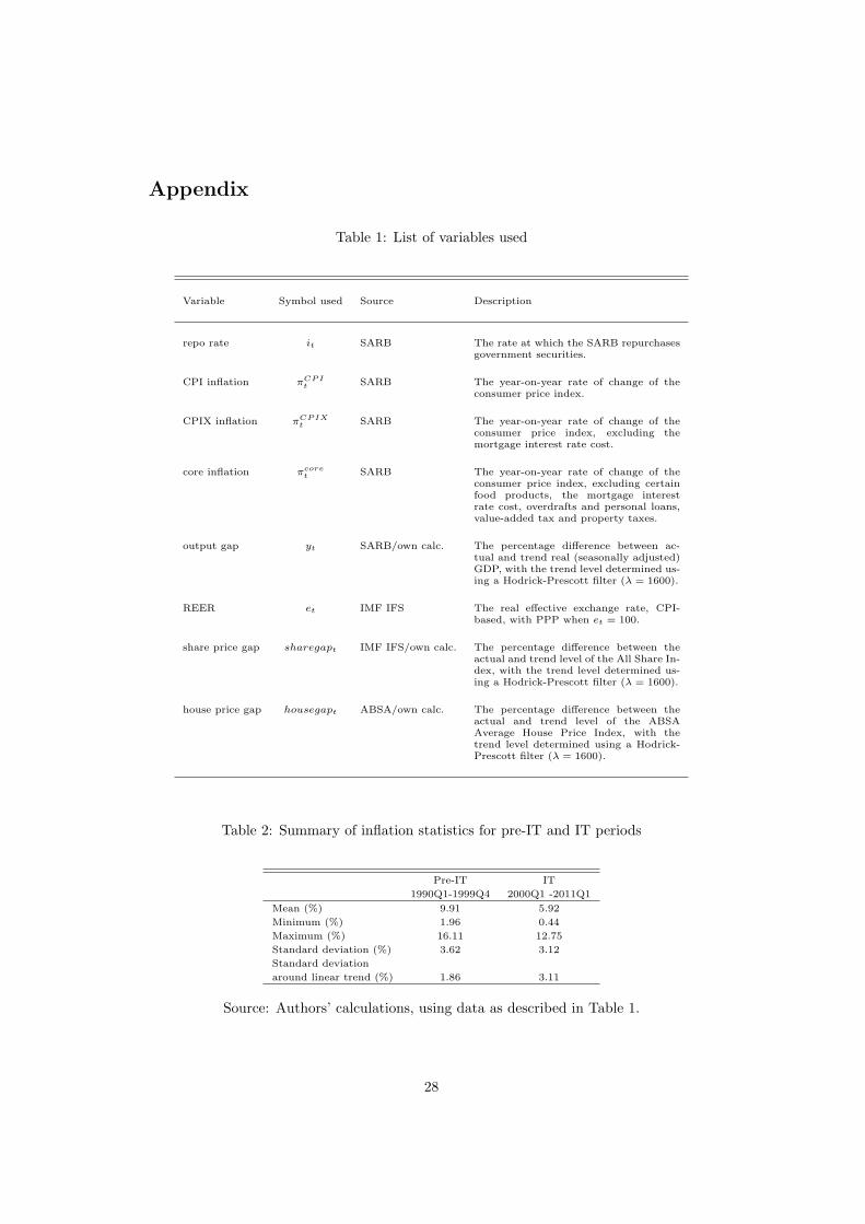
Appendix

Table 1: List of variables used

Variable Symbol used Source Description

repo rate it SARB The rate at which the SARB repurchasesgovernment securities.

CPI inflation πCPIt SARB The year-on-year rate of change of the

consumer price index.

CPIX inflation πCPIXt SARB The year-on-year rate of change of the

consumer price index, excluding themortgage interest rate cost.

core inflation πcoret SARB The year-on-year rate of change of the

consumer price index, excluding certainfood products, the mortgage interestrate cost, overdrafts and personal loans,value-added tax and property taxes.

output gap yt SARB/own calc. The percentage difference between ac-tual and trend real (seasonally adjusted)GDP, with the trend level determined us-ing a Hodrick-Prescott filter (λ = 1600).

REER et IMF IFS The real effective exchange rate, CPI-based, with PPP when et = 100.

share price gap sharegapt IMF IFS/own calc. The percentage difference between theactual and trend level of the All Share In-dex, with the trend level determined us-ing a Hodrick-Prescott filter (λ = 1600).

house price gap housegapt ABSA/own calc. The percentage difference between theactual and trend level of the ABSAAverage House Price Index, with thetrend level determined using a Hodrick-Prescott filter (λ = 1600).

Table 2: Summary of inflation statistics for pre-IT and IT periods

Pre-IT IT

1990Q1-1999Q4 2000Q1 -2011Q1

Mean (%) 9.91 5.92

Minimum (%) 1.96 0.44

Maximum (%) 16.11 12.75

Standard deviation (%) 3.62 3.12

Standard deviation

around linear trend (%) 1.86 3.11

Source: Authors’ calculations, using data as described in Table 1.

28

Table 3: Results of tests for unit root processes in the variables

H0: variable has a unit root

Standard DF test Aug. DF test - 1 lag Aug. DF test - 2 lags

θ |t| θ |t| θ |t|

repot −0.032 1.07 −0.053 1.89 −0.041 1.46

repot (pre-IT) −0.136 1.56 −0.211 2.45 −0.179 1.93

repot (IT) −0.049 0.88 −0.104 2.28 −0.093 1.97

πCPIt −0.082 2.07 −0.109∗∗ 3.10 −0.103∗ 2.79

πCPIt (pre-IT) −0.038 0.58 −0.069 1.04 −0.061 0.90

πCPIt (IT) −0.128 1.81 −0.205∗∗∗ 3.84 −0.199∗∗ 3.14

πCPIXt (IT) −0.037 0.50 −0.156 2.09 −0.190 2.32

πcoret (IT) −0.040 0.51 −0.140 1.63 −0.174 1.87

yt −0.090 2.13 −0.126∗∗∗ 3.75 −0.122∗∗ 3.40

yt (pre-IT) −0.095 1.58 −0.114 2.29 −0.112 2.11

yt (IT) −0.085 1.38 −0.143∗∗ 3.06 −0.138∗ 2.65

et −0.054 1.61 −0.062 1.86 −0.057 1.69

et (pre-IT) −0.054 0.77 −0.066 0.88 −0.039 0.50

et (IT) −0.119 1.58 −0.164 2.15 −0.167 2.02

sharegapt −0.215∗∗ 3.15 −0.270∗∗∗ 3.85 −0.271∗∗ 3.54

sharegapt (pre-IT) −0.332∗ 2.78 −0.422∗∗ 3.33 −0.397∗ 2.72

sharegapt (IT) −0.171 1.98 −0.218 2.47 −0.235 2.47

housegapt −0.065 1.60 −0.117∗∗∗ 3.87 −0.082∗ 2.61

housegapt (pre-IT) −0.140 1.53 −0.294∗∗∗ 4.44 −0.291∗∗∗ 3.55

housegapt (IT) −0.054 1.07 −0.095 2.57 −0.059 1.59

The standard Dickey-Fuller (DF) test is applied by estimating the regression:∆xt = α+ θxt−1 + et, so that θ is the first order autocorrelation of x. The augmentedDF tests add lags of ∆x to the above regression. A value for θ that is statistically sig-nificantly different from zero is evidence against x being a unit root process. The valuesfor θ, as well as their corresponding t-values, are reported. ∗,∗∗ ,∗∗∗ represent statisticallysignificant difference from zero at the 10%, 5% and 1% levels respectively, according tothe Dickey-Fuller distribution (Dickey and Fuller, 1979).

29

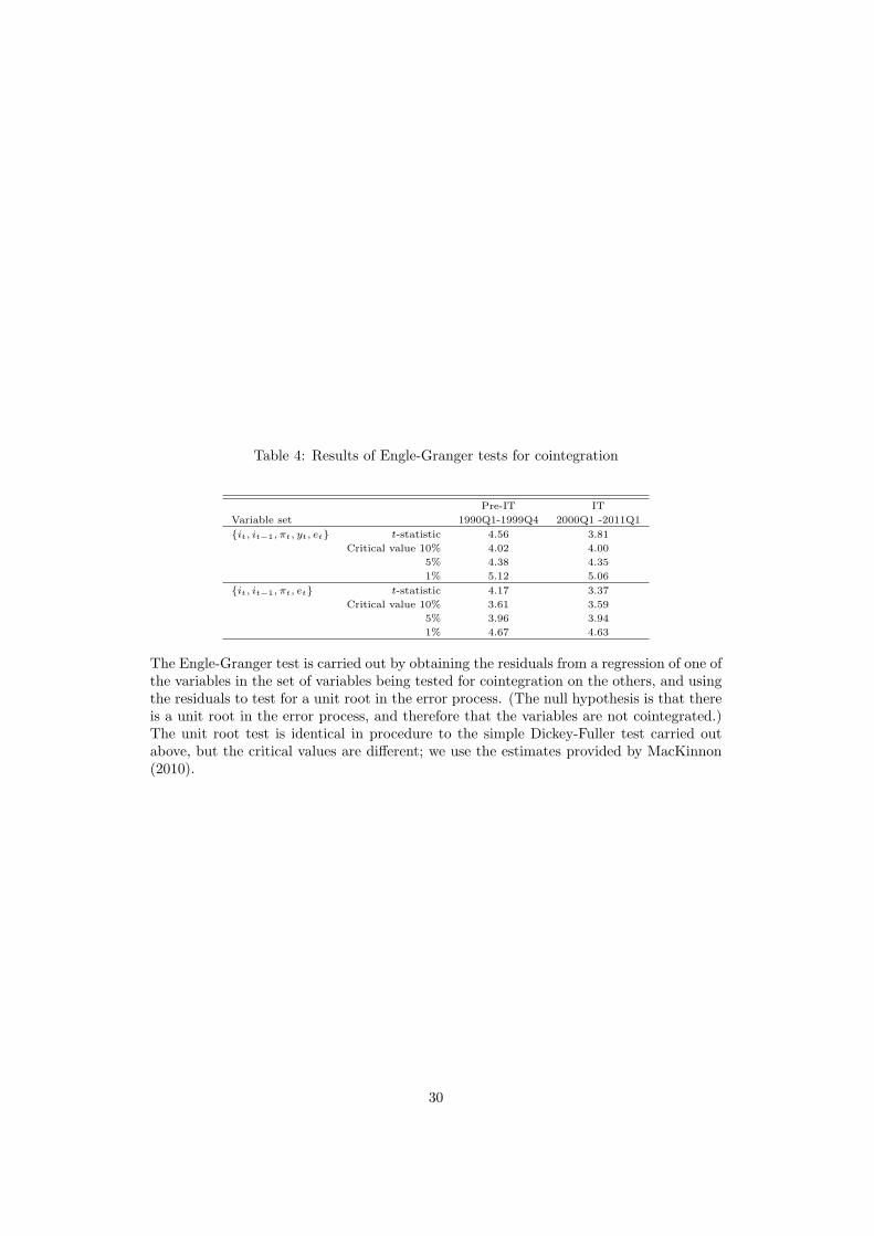
Table 4: Results of Engle-Granger tests for cointegration

Pre-IT IT

Variable set 1990Q1-1999Q4 2000Q1 -2011Q1

{it, it−1, πt, yt, et} t-statistic 4.56 3.81

Critical value 10% 4.02 4.00

5% 4.38 4.35

1% 5.12 5.06

{it, it−1, πt, et} t-statistic 4.17 3.37

Critical value 10% 3.61 3.59

5% 3.96 3.94

1% 4.67 4.63

The Engle-Granger test is carried out by obtaining the residuals from a regression of one ofthe variables in the set of variables being tested for cointegration on the others, and usingthe residuals to test for a unit root in the error process. (The null hypothesis is that thereis a unit root in the error process, and therefore that the variables are not cointegrated.)The unit root test is identical in procedure to the simple Dickey-Fuller test carried outabove, but the critical values are different; we use the estimates provided by MacKinnon(2010).

30

Table 5: Regression results

Dependent variable: ∆repot

Regression: (i) (ii) (iii) (iv) (v) (vi) (vii) (viii) (ix)

Start: 1990Q1 2000Q1 1990Q1 2000Q1 1990Q1 2000Q1 2000Q1 2000Q1 2000Q1

End: 1999Q4 2011Q1 1999Q4 2011Q1 1999Q4 2011Q1 2008Q4 2008Q4 2008Q4

Obs: 40 45 40 45 40 45 36 36 36

∆repot−1 - - 0.175 0.252∗∗ 0.235 0.306∗∗ 0.225 0.349∗∗ 0.405∗∗

(0.173) (0.113) (0.197) (0.132) (0.177) (0.155) (0.163)

∆πCPIt 0.322∗∗ 0.302∗∗∗ 0.247 0.218∗∗∗ 0.272∗ 0.199∗∗∗ 0.205∗∗ - -

(0.137) (0.063) (0.156) (0.071) (0.141) (0.070) (0.083)

∆πCPIXt - - - - - - - 0.271∗∗ -

(0.108)

∆πcoret - - - - - - - - 0.150

(0.102)

∆yt −0.014 0.574∗∗∗ 0.055 0.570∗∗∗ −0.394 0.476∗∗ 0.636∗ 0.548 0.693∗

(0.327) (0.167) (0.334) (0.160) (0.324) (0.207) (0.324) (0.334) (0.347)

∆et - - - - −0.135∗∗∗ −0.030∗ −0.018 −0.028 −0.034

(0.047) (0.016) (0.020) (0.020) (0.021)

∆sharegapt - - - - 0.066∗∗ 0.012 0.012 0.013 0.013

(0.031) (0.011) (0.012) (0.012) (0.013)

∆housegapt - - - - 0.123 −0.019 −0.117 −0.057 −0.068

(0.118) (0.060) (0.086) (0.080) (0.092)

φπ 0.322∗∗ 0.302∗∗∗ 0.299∗ 0.292∗∗∗ 0.356∗∗ 0.286∗∗∗ 0.265∗∗∗ 0.417∗∗ 0.253

φπ − 1 −0.678∗∗∗ −0.698∗∗∗ −0.701∗∗∗ −0.708∗∗∗ −0.644∗∗∗ −0.714∗∗∗ −0.735∗∗∗ −0.583∗∗∗ −0.747∗∗∗

(0.137) (0.063) (0.169) (0.080) (0.162) (0.087) (0.086) (0.163) (0.165)

φy −0.014 0.574∗∗∗ 0.066 0.762∗∗∗ −0.514 0.685∗∗ 0.820∗∗ 0.842∗ 1.165∗∗

(0.327) (0.167) (0.408) (0.242) (0.439) (0.280) (0.393) (0.465) (0.516)

R2 0.127 0.599 0.150 0.642 0.388 0.680 0.659 0.658 0.614

adj. R2 0.081 0.581 0.081 0.616 0.280 0.630 0.591 0.590 0.536

ρ 0.224 0.058 0.122 −0.114 0.088 −0.146 −0.117 −0.185 −0.078

P > |t| 0.161 0.705 0.447 0.452 0.581 0.333 0.502 0.289 0.651

DW d-stat. 1.542 1.691 1.738 2.061 1.733 2.121 2.100 2.216 2.066

Standard errors are reported in parentheses. Statistical significance at the 10%, 5% and 1% significance levels represented by ∗,∗∗ and ∗∗∗

respectively. Output, share price, oil price and house price gaps calculated using a Hodrick-Prescott filter, λ = 1600, and are representedas percentages of the trend. ρ is the estimated coefficient in a regression of the residual on its lagged value; a value for ρ that is statisticallysignificantly different from zero is evidence of serial correlation in the error terms. (None exists here.)

31