What HMMs Can Do

Jeff Bilmesbilmes@ee.washington.edu

Dept of EE, University of WashingtonSeattle WA, 98195-2500

ElectricalElectricalEngineeringEngineering

UWUW

UWEE Technical ReportNumber UWEETR-2002-0003January 2002

Department of Electrical EngineeringUniversity of WashingtonBox 352500Seattle, Washington 98195-2500PHN: (206) 543-2150FAX: (206) 543-3842URL: http://www.ee.washington.edu

What HMMs Can Do

Jeff Bilmesbilmes@ee.washington.edu

Dept of EE, University of WashingtonSeattle WA, 98195-2500

University of Washington, Dept. of EE, UWEETR-2002-0003

January 2002

Abstract

Since their inception over thirty years ago, hidden Markov models (HMMs) have have become the predominantmethodology for automatic speech recognition (ASR) systems — today, most state-of-the-art speech systems areHMM-based. There have been a number of ways to explain HMMs and to list their capabilities, each of theseways having both advantages and disadvantages. In an effort to better understand what HMMs can do, this tutorialanalyzes HMMs by exploring a novel way in which an HMM can be defined, namely in terms of random variables andconditional independence assumptions. We prefer this definition as it allows us to reason more throughly about thecapabilities of HMMs. In particular, it is possible to deduce that there are, in theory at least, no theoretical limitationsto the class of probability distributions representable by HMMs. This paper concludes that, in search of a modelto supersede the HMM for ASR, we should rather than trying to correct for HMM limitations in the general case,new models should be found based on their potential for better parsimony, computational requirements, and noiseinsensitivity.

1 IntroductionBy and large, automatic speech recognition (ASR) has been approached using statistical pattern classification [29,24, 36], mathematical methodology readily available in 1968, and summarized as follows: given data presumablyrepresenting an unknown speech signal, a statistical model of one possible spoken utterance (out of a potentially verylarge set) is chosen that most probably explains this data. This requires, for each possible speech utterance, a modelgoverning the set of likely acoustic conditions that could realize each utterance.

More than any other statistical technique, the Hidden Markov model (HMM) has been most successfully appliedto the ASR problem. There have been many HMM tutorials [69, 18, 53]. In the widely read and now classic paper[86], an HMM is introduced as a collection of urns each containing a different proportion of colored balls. Sampling(generating data) from an HMM occurs by choosing a new urn based on only the previously chosen urn, and thenchoosing with replacement a ball from this new urn. The sequence of urn choices are not made public (and are said tobe “hidden”) but the ball choices are known (and are said to be “observed”). Along this line of reasoning, an HMM canbe defined in such a generative way, where one first generates a sequence of hidden (urn) choices, and then generatesa sequence of observed (ball) choices.

For statistical speech recognition, one is not only worried in how HMMs generate data, but also, and more impor-tantly, in an HMMs distributions over observations, and how those distributions for different utterances compare witheach other. An alternative view of HMMs, therefore and as presented in this paper, can provide additional insight intowhat the capabilities of HMMs are, both in how they generate data and in how they might recognize and distinquishbetween patterns.

This paper therefore provides an up-to-date HMM tutorial. It gives a precise HMM definition, where an HMM isdefined as a variable-size collection of random variables with an appropriate set of conditional independence proper-ties. In an effort to better understand what HMMs can do, this paper also considers a list of properties, and discusseshow they each might or might not apply to an HMM. In particular, it will be argued that, at least within the paradigm

1

offered by statistical pattern classification [29, 36], there is no general theoretical limit to HMMs given enough hiddenstates, rich enough observation distributions, sufficient training data, adequate computation, and appropriate trainingalgorithms. Instead, only a particular individual HMM used in a speech recognition system might be inadequate. Thisperhaps provides a reason for the continual speech-recognition accuracy improvements we have seen with HMM-basedsystems, and for the difficulty there has been in producing a model to supersede HMMs.

This paper does not argue, however, that HMMs should be the final technology for speech recognition. On thecontrary, a main hope of this paper is to offer a better understanding of what HMMs can do, and consequently, abetter understanding of their limitations so they may ultimately be abandoned in favor of a superior model. Indeed,HMMs are extremely flexible and might remain the preferred ASR method for quite some time. For speech recognitionresearch, however, a main thrust should be searching for inherently more parsimonious models, ones that incorporateonly the distinct properties of speech utterances relative to competing speech utterances. This later property is termedstructural discriminability [8], and refers to a generative model’s inherent inability to represent the properties of datacommon to every class, even when trained using a maximum likelihood parameter estimation procedure. This meansthat even if a generative model only poorly represents speech, leading to low probability scores, it may still properlyclassify different speech utterances. These models are to be called discriminative generative models.

Section 2 reviews random variables, conditional independence, and graphical models (Section 2.1), stochasticprocesses (Section 2.2), and discrete-time Markov chains (Section 2.3). Section 3 provides a formal definition ofan HMM, that has both a generative and an “acceptive” point of view. Section 4 compiles a list of properties, anddiscusses how they might or might not apply to HMMs. Section 5 derives conditions for HMM accuracy in a Kullback-Leibler distance sense, proving a lower bound on the necessary number of hidden states. The section derives sufficientconditions as well. Section 6 reviews several alternatives to HMMs, and concludes by presenting an intuitive criterionone might use when researching HMM alternatives

1.1 NotationMeasure theoretic principles are avoided in this paper, and discrete and continuous random variables are distinguishedonly where necessary. Capital letters (e.g., X , Q) will refer to random variables, lower case letters (e.g., x, q) will referto values of those random variables, and script letters (e.q., X, Q) will refer to possible values so that x ∈ X, q ∈ Q.If X is distributed according to p, it will be written X ∼ p(X). Probabilities are denoted pX(X = x), p(X = x), orp(x) which are equivalent. For notational simplicity, p(x) will at different times symbolize a continuous probabilitydensity or a discrete probability mass function. The distinction will be unambiguous when needed.

It will be necessary to refer to sets of integer indexed random variables. Let A∆= {a1, a2, . . . , aN} be a set

of T integers. Then XA∆= {Xa1

, Xa2, . . . , XaT

}. If B ⊂ A then XB ⊂ XA. It will also be useful to definesets of integers using matlab-like ranges. As such, Xi:j with i < j will refer to the variables Xi, Xi+1, . . . , Xj .

X<i∆= {X1, X2, . . . , Xi−1}, and X¬t

∆= X1:T \ Xt = {X1, X2, . . . , Xt−1, Xt+1, Xt+2, . . . , XT } where T will be

clear from the context, and \ is the set difference operator. When referring to sets of T random variable, it will also beuseful to define X

∆= X1:T and x

∆= x1:T . Additional notation will be defined when needed.

2 PreliminariesBecause within an HMM lies a hidden Markov chain which in turn contains a sequence of random variables, it isuseful to review a few noteworthy prerequisite topics before beginning an HMM analysis. Some readers may wish toskip directly to Section 3. Information theory, while necessary for a later section of this paper, is not reviewed and thereader is referred to the texts [16, 42].

2.1 Random Variables, Conditional Independence, and Graphical ModelsA random variable takes on values (or in the continuous case, a range of values) with certain probabilities.1 Differ-ent random variables might or might not have the ability to influence each other, a notion quantified by statisticalindependence. Two random variables X and Y are said to be (marginally) statistically independent if and only if

1In this paper, explanations often use discrete random variables to avoid measure theoretic notation needed in the continuous case. See [47, 103,2] for a precise treatment of continuous random variables. Note also that random variables may be either scalar or vector valued.

UWEETR-2002-0003 2

p(X = x, Y = y) = p(X = x)p(Y = y) for every value of x and y. This is written X⊥⊥Y . Independence impliesthat regardless of the outcome of one random variable, the probabilities of the outcomes of the other random variablestay the same.

Two random variables might or might not be independent of each other depending on knowledge of a third randomvariable, a concept captured by conditional independence. A random variable X is conditionally independent ofa different random variable Y given a third random variable Z under a given probability distribution p(·), if thefollowing relation holds:

p(X = x, Y = y|Z = z) = p(X = x|Z = z)p(Y = y|Z = z)

for all x, y, and z. This is written X⊥⊥Y |Z and it is said that “X is independent of Y given Z under p(·)”. Anequivalent definition is p(X = x|Y = y, Z = z) = p(X = x|Z = z). The conditional independence of Xand Y given Z has the following intuitive interpretation: if one has knowledge of Z, then knowledge of Y doesnot change one’s knowledge of X and vice versa. Conditional independence is different from unconditional (ormarginal) independence. Therefore, it might be true that X⊥⊥Y but not true that X⊥⊥Y |Z. One valuable property ofconditional independence follows: if XA⊥⊥YB |ZC , and subsets A′ ⊂ A and B′ ⊂ B are formed, then it follows thatXA′⊥⊥YB′ |ZC . Conditional independence is a powerful concept — when assumptions are made, a statistical modelcan undergo enormous simplifications. Additional properties of conditional independence are presented in [64, 81].

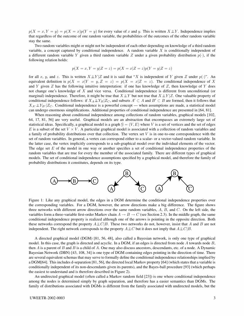
When reasoning about conditional independence among collections of random variables, graphical models [102,64, 17, 81, 56] are very useful. Graphical models are an abstraction that encompasses an extremely large set ofstatistical ideas. Specifically, a graphical model is a graph G = (V,E) where V is a set of vertices and the set of edgesE is a subset of the set V × V . A particular graphical model is associated with a collection of random variables anda family of probability distributions over that collection. The vertex set V is in one-to-one correspondence with theset of random variables. In general, a vertex can correspond either to a scalar- or a vector-valued random variable. Inthe latter case, the vertex implicitly corresponds to a sub-graphical model over the individual elements of the vector.The edge set E of the model in one way or another specifies a set of conditional independence properties of therandom variables that are true for every the member of the associated family. There are different types of graphicalmodels. The set of conditional independence assumptions specified by a graphical model, and therefore the family ofprobability distributions it constitutes, depends on its type.

A B C A

B

C A

B

C

Figure 1: Like any graphical model, the edges in a DGM determine the conditional independence properties overthe corresponding variables. For a DGM, however, the arrow directions make a big difference. The figure showsthree networks with different arrow directions over the same random variables, A, B, and C. On the left side, thevariables form a three-variable first-order Markov chain A → B → C (see Section 2.3). In the middle graph, the sameconditional independence property is realized although one of the arrows is pointing in the opposite direction. Boththese networks correspond the property A⊥⊥C|B. These two networks do not, however, insist that A and B are notindependent. The right network corresponds to the property A⊥⊥C but it does not imply that A⊥⊥C|B.

A directed graphical model (DGM) [81, 56, 48], also called a Bayesian network, is only one type of graphicalmodel. In this case, the graph is directed and acyclic. In a DGM, if an edges is directed from node A towards node B,then A is a parent of B and B is a child of A. One may also discuss ancestors, descendants, etc. of a node. A DynamicBayesian Network (DBN) [43, 108, 34] is one type of DGM containing edges pointing in the direction of time. Thereare several equivalent schemas that may serve to formally define the conditional independence relationships implied bya DGM[64]. This includes d-separation [81, 56], the directed local Markov property [64] (which states that a variable isconditionally independent of its non-descendants given its parents), and the Bayes-ball procedure [93] (which perhapsthe easiest to understand and is therefore described in Figure 2).

An undirected graphical model (often called a Markov random field [23]) is one where conditional independenceamong the nodes is determined simply by graph separation, and therefore has a easier semantics than DGMs. Thefamily of distributions associated with DGMs is different from the family associated with undirected models, but the

UWEETR-2002-0003 3

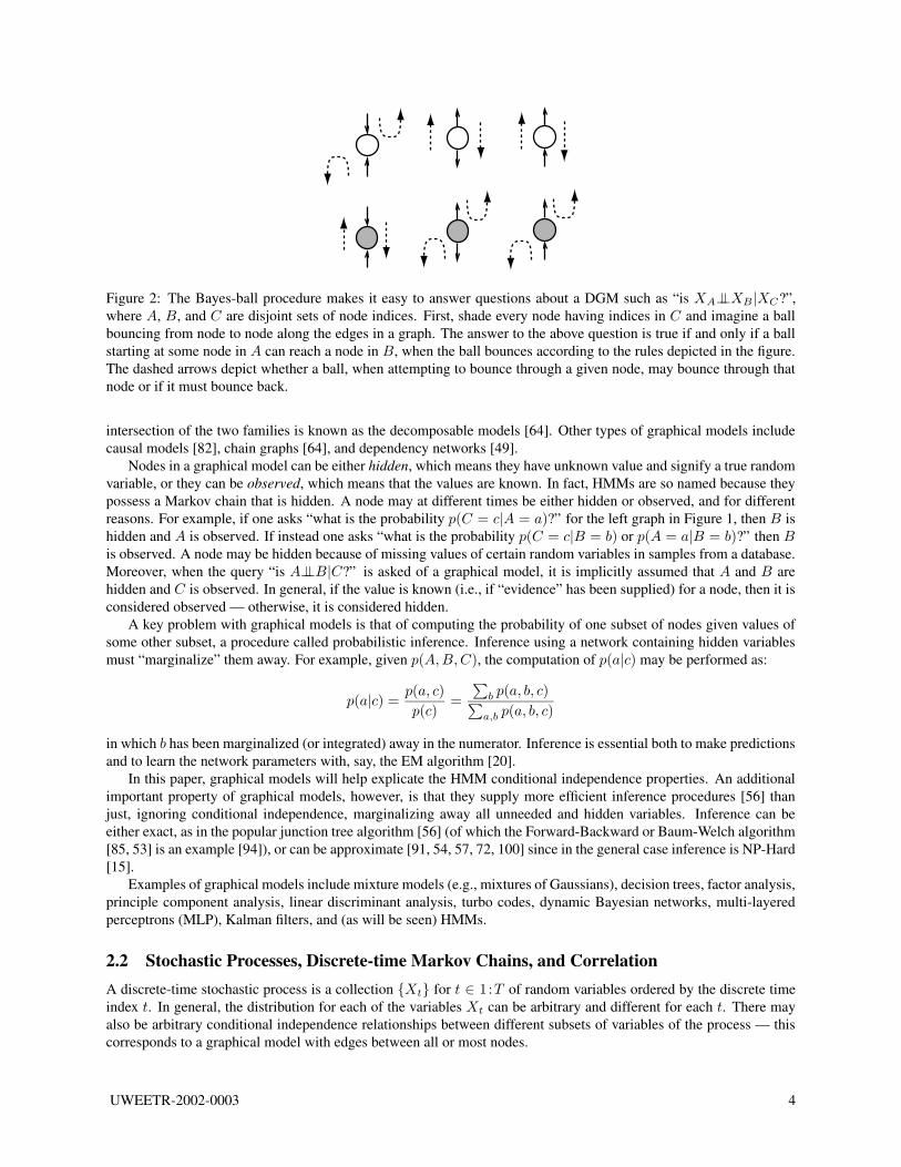
Figure 2: The Bayes-ball procedure makes it easy to answer questions about a DGM such as “is XA⊥⊥XB |XC?”,where A, B, and C are disjoint sets of node indices. First, shade every node having indices in C and imagine a ballbouncing from node to node along the edges in a graph. The answer to the above question is true if and only if a ballstarting at some node in A can reach a node in B, when the ball bounces according to the rules depicted in the figure.The dashed arrows depict whether a ball, when attempting to bounce through a given node, may bounce through thatnode or if it must bounce back.

intersection of the two families is known as the decomposable models [64]. Other types of graphical models includecausal models [82], chain graphs [64], and dependency networks [49].

Nodes in a graphical model can be either hidden, which means they have unknown value and signify a true randomvariable, or they can be observed, which means that the values are known. In fact, HMMs are so named because theypossess a Markov chain that is hidden. A node may at different times be either hidden or observed, and for differentreasons. For example, if one asks “what is the probability p(C = c|A = a)?” for the left graph in Figure 1, then B ishidden and A is observed. If instead one asks “what is the probability p(C = c|B = b) or p(A = a|B = b)?” then Bis observed. A node may be hidden because of missing values of certain random variables in samples from a database.Moreover, when the query “is A⊥⊥B|C?” is asked of a graphical model, it is implicitly assumed that A and B arehidden and C is observed. In general, if the value is known (i.e., if “evidence” has been supplied) for a node, then it isconsidered observed — otherwise, it is considered hidden.

A key problem with graphical models is that of computing the probability of one subset of nodes given values ofsome other subset, a procedure called probabilistic inference. Inference using a network containing hidden variablesmust “marginalize” them away. For example, given p(A,B,C), the computation of p(a|c) may be performed as:

p(a|c) =p(a, c)

p(c)=

∑

b p(a, b, c)∑

a,b p(a, b, c)

in which b has been marginalized (or integrated) away in the numerator. Inference is essential both to make predictionsand to learn the network parameters with, say, the EM algorithm [20].

In this paper, graphical models will help explicate the HMM conditional independence properties. An additionalimportant property of graphical models, however, is that they supply more efficient inference procedures [56] thanjust, ignoring conditional independence, marginalizing away all unneeded and hidden variables. Inference can beeither exact, as in the popular junction tree algorithm [56] (of which the Forward-Backward or Baum-Welch algorithm[85, 53] is an example [94]), or can be approximate [91, 54, 57, 72, 100] since in the general case inference is NP-Hard[15].

Examples of graphical models include mixture models (e.g., mixtures of Gaussians), decision trees, factor analysis,principle component analysis, linear discriminant analysis, turbo codes, dynamic Bayesian networks, multi-layeredperceptrons (MLP), Kalman filters, and (as will be seen) HMMs.

2.2 Stochastic Processes, Discrete-time Markov Chains, and CorrelationA discrete-time stochastic process is a collection {Xt} for t ∈ 1:T of random variables ordered by the discrete timeindex t. In general, the distribution for each of the variables Xt can be arbitrary and different for each t. There mayalso be arbitrary conditional independence relationships between different subsets of variables of the process — thiscorresponds to a graphical model with edges between all or most nodes.

UWEETR-2002-0003 4

Certain types of stochastic processes are common because of their analytical and computational simplicity. Oneexample follows:

Definition 2.1. Independent and Identically Distributed (i.i.d.) The stochastic process is said to be i.i.d.[16, 80, 26]if the following condition holds:

p(Xt = xt, Xt+1 = xt+1, . . . , Xt+h = xt+h) =h∏

i=0

p(X = xt+i) (1)

for all t, for all h ≥ 0, for all xt:t+h, and for some distribution p(·) that is independent of the index t.

An i.i.d. process therefore comprises an ordered collection of independent random variables each one havingexactly the same distribution. A graphical model of an ı.i.d process contains no edges at all.

If the statistical properties of variables within a time-window of a stochastic process do not evolve over time, theprocess is said to be stationary.

Definition 2.2. Stationary Stochastic Process The stochastic process {Xt : t ≥ 1} is said to be (strongly) stationary[47] if the two collections of random variables

{Xt1 , Xt2 , . . . , Xtn}

and{Xt1+h, Xt2+h, . . . , Xtn+h}

have the same joint probability distributions for all n and h.

In the continuous case, stationarity means that FXt1:n(a) = FXt1:n+h

(a) for all a where F (·) is the cumulativedistribution and a is a valid vector-valued constant of length n. In the discrete case, stationarity is equivalent to thecondition

P (Xt1 = x1, Xt2 = x2, . . . , Xtn= xn) = P (Xt1+h = x1, Xt2+h = x2, . . . , Xtn+h = xn)

for all t1, t2, . . . , tn, for all n > 0, for all h > 0, and for all xi. Every i.i.d. processes is stationary.The covariance between two random vectors X and Y is defined as:

cov(X,Y ) = E[(X − EX)(Y − EY )′] = E(XY ′) − E(X)E(Y )′

It is said that X and Y are uncorrelated if cov(X,Y ) = ~0 (equivalently, if E(XY ′) = E(X)E(Y )′) where ~0 is thezero matrix. If X and Y are independent, then they are uncorrelated, but not vice versa unless they are jointly Gaussian[47].

2.3 Markov ChainsA collection of discrete-valued random variables {Qt :≥ 1} forms an nth-order Markov chain [47] if

P (Qt = qt|Qt−1 = qt−1, Qt−2 = qt−2, . . . , Q1 = q1)

= P (Qt = qt|Qt−1 = qt−1, Qt−2 = qt−2, . . . , Qt−n = qt−n)

for all t ≥ 1, and all q1, q2, . . . , qt. In other words, given the previous n random variables, the current variable isconditionally independent of every variable earlier than the previous n. A first order Markov chain is depicted usingthe left network in Figure 1.

One often views the event {Qt = i} as if the chain is “in state i at time t” and the event {Qt = i, Qt+1 = j}as a transition from state i to state j starting at time t. This notion arises by viewing a Markov chain as a finite-state automata (FSA) [52] with probabilistic state transitions. In this case, the number of states corresponds to thecardinality of each random variable. In general, a Markov chain may have infinitely many states, but chain variablesin this paper are assumed to have only finite cardinality.

UWEETR-2002-0003 5

An nth-order Markov chain may always be converted into an equivalent first-order Markov chain [55] using thefollowing procedure:

Q′t

∆= {Qt, Qt−1, . . . , Qt−n}

where Qt is an nth-order Markov chain. Then Q′t is a first-order Markov chain because

P (Q′t = q′t|Q

′t−1 = q′t−1, Q

′t−2 = q′t−2, . . . , Q

′1 = q′1)

= P (Qt−n:t = qt−n:t|Q1:t = q1:t)

= P (Qt−n:t = qt−n:t|Qt−n−1:t = qt−n−1:t)

= P (Q′t = q′t|Q

′t−1 = q′t−1)

This transformation implies that, given a large enough state space, a first-order Markov chain may represent anynth-order Markov chain.

The statistical evolution of a Markov chain is determined by the state transition probabilities aij(t)∆= P (Qt =

j|Qt−1 = i). In general, the transition probabilities can be a function both of the states at successive time steps and ofthe current time t. In many cases, it is assumed that there is no such dependence on t. Such a time-independent chainis called time-homogeneous (or just homogeneous) because aij(t) = aij for all t.

The transition probabilities in a homogeneous Markov chain are determined by a transition matrix A where aij∆=

(A)ij . The rows of A form potentially different probability mass functions over the states of the chain. For this reason,A is also called a stochastic transition matrix (or just a transition matrix).

A state of a Markov chain may be categorized into one of three distinct categories [47]. A state i is said to betransient if, after visiting the state, it is possible for it never to be visited again, i.e.,:

p(Qn = i for some n > t|Qt = i) < 1.

A state i is said to be null-recurrent if it is not transient but the expected return time is infinite (i.e., E[min{n >t : Qn = i}|Qt = i] = ∞). Finally, a state is positive-recurrent if it is not transient and the expected returntime to that state is finite. For a Markov chain with a finite number of states, a state can only be either transient orpositive-recurrent.

Like any stochastic process, an individual Markov chain might or might not be a stationary process. The station-arity condition of a Markov chain, however, depends on 1) if the Markov chain transition matrix has (or “admits”) astationary distribution or not, and 2) if the current distribution over states is one of those stationary distributions.

If Qt is a time-homogeneous stationary Markov chain then:

P (Qt1 = q1, Qt2 = q2, . . . , Qtn= qn) = P (Qt1+h = q1, Qt2+h = q2, . . . , Qtn+h = qn)

for all ti, h, n, and qi. Using the first order Markov property, the above can be written as:

P (Qtn= qn|Qtn−1

= qn−1)P (Qtn−1= qn−1|Qtn−2

= qn−2) . . .

P (Qt2 = q2|Qt1 = q1)P (Qt1 = q1)

= P (Qtn+h = qn|Qtn−1+h = qn−1)P (Qtn−1+h = qn−1|Qtn−2+h = qn−2) . . .

P (Qt2+h = q2|Qt1+h = q1)P (Qt1+h = q1)

Therefore, a homogeneous Markov chain is stationary only when P (Qt1 = q) = P (Qt1+h = q) = P (Qt = q) for allq ∈ Q. This is called a stationary distribution of the Markov chain and will be designated by ξ with ξi = P (Qt = i).2

According to the definition of the transition matrix, a stationary distribution has the property that ξA = ξ implyingthat ξ must be a left eigenvector of the transition matrix A. For example, let p1 = [.5, .5] be the current distributionover a 2-state Markov chain (using matlab notation). Let A1 = [.3, .7; .7, .3] be the transition matrix. The Markovchain is stationary since p1A1 = p1. If the current distribution is p2 = [.4, .6], however, then p2A1 6= p2, so the chainis no longer stationary.

In general, there can be more than one stationary distribution for a given Markov chain (as there can be more thanone eigenvector of a matrix). The condition of stationarity for the chain, however, depends on if the chain “admits” astationary distribution, and if it does, whether the current marginal distribution over the states is one of the stationary

2This is typically designated using π, but that will be reserved for initial HMM distributions.

UWEETR-2002-0003 6

distributions. If a chain does admit a stationary distribution ξ, then ξj = 0 for all j that are transient and null-recurrent[47]; i.e., a stationary distribution has positive probability only for positive-recurrent states (states that are assuredlyre-visited).

The time-homogeneous property of a Markov chain is distinct from the stationarity property. Stationarity, however,does implies time-homogeneity. To see this, note that if the process is stationary then P (Qt = i, Qt−1 = j) =P (Qt−1 = i, Qt−2 = j) and P (Qt = i) = P (Qt−1 = i). Therefore, aij(t) = P (Qt = i, Qt−1 = j)/P (Qt−1 =j) = P (Qt−1 = i, Qt−2 = j)/P (Qt−2 = j) = aij(t−1), so by induction aij(t) = aij(t+ τ) for all τ , and the chainis time-homogeneous. On the other hand, a time-homogeneous Markov chain might not admit a stationary distributionand therefore never correspond to a stationary random process.

The idea of “probability flow” may help to determine if a Markov chain admits a stationary distribution. Stationary,or ξA = ξ, implies that for all i

ξi =∑

j

ξjaji

or equivalently,ξi(1 − aii) =

∑

j 6=i

ξjaji

which is the same as∑

j 6=i

ξiaij =∑

j 6=i

ξjaji

The left side of this equation can be interpreted as the probability flow out of state i and the right side can be interpretedas the flow into state i. A stationary distribution requires that the inflow and outflow cancel each other out for everystate.

3 Hidden Markov ModelsWe at last arrive at the main topic of this paper. As will be seen, an HMM is a statistical model for a sequence of dataitems called the observation vectors. Rather than wet our toes with HMM general properties and analogies, we diveright in by providing a formal definition.

Definition 3.1. Hidden Markov Model A hidden Markov model (HMM) is collection of random variables consistingof a set of T discrete scalar variables Q1:T and a set of T other variables X1:T which may be either discrete orcontinuous (and either scalar- or vector-valued). These variables, collectively, possess the following conditionalindependence properties:

{Qt:T , Xt:T }⊥⊥{Q1:t−2, X1:t−1}|Qt−1 (2)

andXt⊥⊥{Q¬t, X¬t}|Qt (3)

for each t ∈ 1 : T . No other conditional independence properties are true in general, unless they follow fromEquations 2 and 3. The length T of these sequences is itself an integer-valued random variable having a complexdistribution (see Section 4.7).

Let us suppose that each Qt may take values in a finite set, so Qt ∈ Q where Q is called the state space which hascardinality |Q|. A number of HMM properties may immediately be deduced from this definition.

Equations (2) and (3) imply a large assortment of conditional independence statements. Equation 2 states that thefuture is conditionally independent of the past given the present. One implication3 is that Qt⊥⊥Q1:t−2|Qt−1 whichmeans the variables Q1:T form a discrete-time, discrete-valued, first-order Markov chain. Another implication ofEquation 2 is Qt⊥⊥{Q1:t−2, X1:t−1}|Qt−1 which means that Xτ is unable, given Qt−1, to affect Qt for τ < t. Thisdoes not imply, given Qt−1, that Qt is unaffected by future variables. In fact, the distribution of Qt could dramaticallychange, even given Qt−1, when the variables Xτ or Qτ+1 change, for τ > t.

The other variables X1:T form a general discrete time stochastic process with, as we will see, great flexibil-ity. Equation 3 states that given an assignment to Qt, the distribution of Xt is independent of every other variable

3Recall Section 2.1.

UWEETR-2002-0003 7

(both in the future and in the past) in the HMM. One implication is that Xt⊥⊥Xt+1|{Qt, Qt+1} which follows sinceXt⊥⊥{Xt+1, Qt+1}|Qt and Xt⊥⊥Xt+1|Qt+1.

Definition 3.1 does not limit the number of states |Q| in the Markov chain, does not require the observations X1:T

to be either discrete, continuous, scalar-, or vector- valued, does not designate the implementation of the dependencies(e.g., general regression, probability table, neural network, etc.), does not determine the model families for each ofthe variables (e.g., Gaussian, Laplace, etc.), does not force the underlying Markov chain to be time-homogeneous, anddoes not fix the parameters or any tying mechanism.

Any joint probability distribution over an appropriately typed set of random variables that obeys the above set ofconditional independence rules is then an HMM. The two above conditional independence properties imply that, for agiven T , the joint distribution over all the variables may be expanded as follows:

p(x1:T , q1:T ) = p(xT , qT |x1:T−1, q1:T−1)p(x1:T−1, q1:T−1) Chain Rule of probability.= p(xT |qT , x1:T−1, q1:T−1)p(qT |x1:T−1, q1:T−1)p(x1:T−1, q1:T−1) Again, chain rule.= p(xT |qT )p(qT |qT−1)p(x1:T−1, q1:T−1) Since XT⊥⊥{X1:T−1, Q1:T−1}|QT

and QT⊥⊥{X1:T−1, Q1:T−2}|QT−1

which follow from Definition 3.1

.

= . . .

= p(q1)

T∏

t=2

p(qt|qt−1)

T∏

t=1

p(xt|qt)

To parameterize an HMM, one therefore needs the following quantities: 1) the distribution over the initial chainvariable p(q1), 2) the conditional “transition” distributions for the first-order Markov chain p(qt|qt−1), and 3) theconditional distribution for the other variables p(xt|qt). It can be seen that these quantities correspond to the classicHMM definition [85]. Specifically, the initial (not necessarily stationary) distribution is labeled π which is a vector oflength |Q|. Then, p(Q1 = i) = πi. where πi is the ith element of π. The observation probability distributions arenotated bj(x) = p(Xt = x|Qt = j) and the associated parameters depend on bj(x)’s family of distributions. Also,the Markov chain is typically assumed to be time-homogeneous, with stochastic matrix A where (A)ij = p(Qt =

j|Qt−1 = i) for all t. HMM parameters are often symbolized collectively as λ∆= (π,A,B) where B represents the

parameters corresponding to all the observation distributions.For speech recognition, the Markov chain Q1:T is typically hidden, which naturally results in the name hidden

Markov model. The variables X1:T are typically observed. These are the conventional variable designations but neednot always hold. For example, Xτ could be missing or hidden, for some or all τ . In some tasks, Q1:T might be knownand X1:T might be hidden. The name “HMM” applies in any case, even if Q1:T are not hidden and X1:T are notobserved. Regardless, Q1:T will henceforth refer to the hidden variables and X1:T the observations.

With the above definition, an HMM can be simultaneously viewed as a generator and a stochastic acceptor. Likeany random variable, say Y , one may obtain a sample from that random variable (e.g., flip a coin), or given a sample,say y, one may compute the probability of that sample p(Y = y) (e.g., the probability of heads). One way to samplefrom an HMM is to first obtain a complete sample from the hidden Markov chain (i.e., sample from all the randomvariables Q1:T by first sampling Q1, then Q2 given Q1, and so on.), and then at each time point t produce a sample ofXt using p(Xt|qt), the observation distribution according to the hidden variable value at time t. This is the same aschoosing first a sequence of urns and then a sequence of balls from each urn as described in [85]. To sample just fromX1:T , one follows the same procedure but then throws away the Markov chain Q1:T .

It is important to realize that each sample of X1:T requires a new and different sample of Q1:T . In other words,two different HMM observation samples typically originate from two different state assignments to the hidden Markovchain. Put yet another way, an HMM observation sample is obtained using the marginal distribution p(X1:T ) =∑

q1:Tp(X1:T , q1:T ) and not from the conditional distribution p(X1:T |q1:t) for some fixed hidden variable assignment

q1:T . As will be seen, this marginal distribution p(X1:T ) can be quite general.Correspondingly, when one observes only the collection of values x1:T , they have presumably been produced

according to some specific but unknown assignment to the hidden variables. A given x1:T , however, could have beenproduced from one of many different assignments to the hidden variables. To compute the probability p(x1:T ), one

UWEETR-2002-0003 8

must therefore marginalize away all possible assignments to Q1:T as follows:

p(x1:T ) =∑

q1:T

p(x1:T , q1:T )

=∑

q1:T

p(q1)

T∏

t=2

p(qt|qt−1)

T∏

t=1

p(xt|qt)

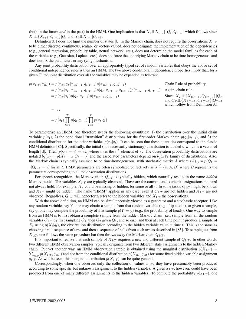
Figure 3: Stochastic finite-state automaton view of an HMM. In this case, only the possible (i.e., non-zero probability)hidden Markov chain state transitions are shown.

An HMM may be graphically depicted in three ways. The first view portrays only a directed state-transition graphas in Figure 3. It is important to realize that this view neither depicts the HMM’s output distributions nor the conditionalindependence properties. The graph depicts only the allowable transitions in the HMM’s underlying Markov chain.Each node corresponds to one of the states in Q, where an edge going from node i to node j indicates that aij > 0,and the lack of such an edge indicates that aij = 0. The transition matrix associated with Figure 3 is as follows:

A =

a11 a12 a13 0 0 0 0 0

0 a22 0 a24 a25 0 0 0

0 0 a33 a34 0 0 a37 0

0 0 0 a44 a45 a46 0 0

0 0 0 0 0 0 a57 0

0 0 0 0 0 0 0 a68

0 a72 0 0 0 0 0 a78

a81 0 0 0 0 0 0 a88

where it is assumed that the explicitly mentioned aij are non-zero. In this view, an HMM is seen as an extendedstochastic FSA [73]. One can envisage being in a particular state j at a certain time, producing an observation samplefrom the observation distribution corresponding to that state bj(x), and then advancing to the next state according tothe non-zero transitions.

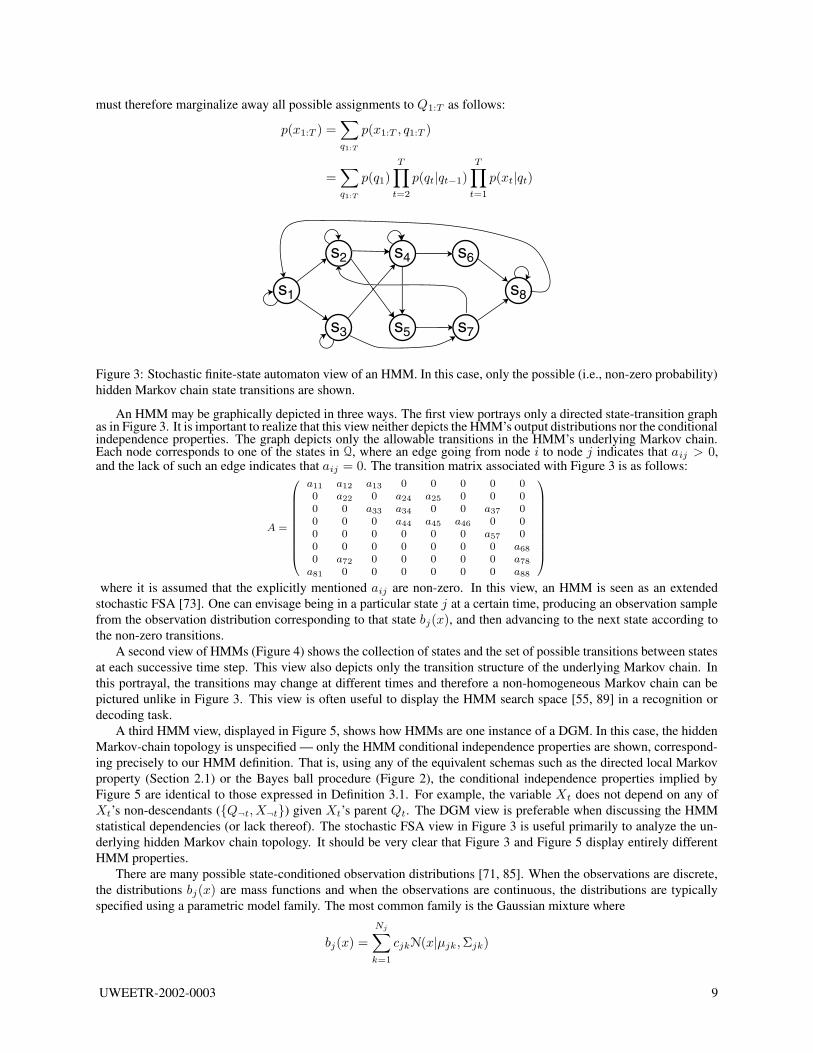
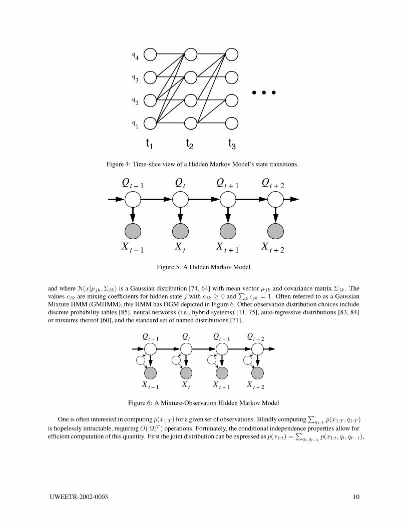
A second view of HMMs (Figure 4) shows the collection of states and the set of possible transitions between statesat each successive time step. This view also depicts only the transition structure of the underlying Markov chain. Inthis portrayal, the transitions may change at different times and therefore a non-homogeneous Markov chain can bepictured unlike in Figure 3. This view is often useful to display the HMM search space [55, 89] in a recognition ordecoding task.

A third HMM view, displayed in Figure 5, shows how HMMs are one instance of a DGM. In this case, the hiddenMarkov-chain topology is unspecified — only the HMM conditional independence properties are shown, correspond-ing precisely to our HMM definition. That is, using any of the equivalent schemas such as the directed local Markovproperty (Section 2.1) or the Bayes ball procedure (Figure 2), the conditional independence properties implied byFigure 5 are identical to those expressed in Definition 3.1. For example, the variable Xt does not depend on any ofXt’s non-descendants ({Q¬t, X¬t}) given Xt’s parent Qt. The DGM view is preferable when discussing the HMMstatistical dependencies (or lack thereof). The stochastic FSA view in Figure 3 is useful primarily to analyze the un-derlying hidden Markov chain topology. It should be very clear that Figure 3 and Figure 5 display entirely differentHMM properties.

There are many possible state-conditioned observation distributions [71, 85]. When the observations are discrete,the distributions bj(x) are mass functions and when the observations are continuous, the distributions are typicallyspecified using a parametric model family. The most common family is the Gaussian mixture where

bj(x) =

Nj∑

k=1

cjkN(x|µjk,Σjk)

UWEETR-2002-0003 9

t1 t2 t3

q1

q2

q3

q4

Figure 4: Time-slice view of a Hidden Markov Model’s state transitions.

Q t Q t 1 + Q t 1 – Q t 2 +

X t X t 1 + X t 1 – X t 2 +

Figure 5: A Hidden Markov Model

and where N(x|µjk,Σjk) is a Gaussian distribution [74, 64] with mean vector µjk and covariance matrix Σjk. Thevalues cjk are mixing coefficients for hidden state j with cjk ≥ 0 and

∑

k cjk = 1. Often referred to as a GaussianMixture HMM (GMHMM), this HMM has DGM depicted in Figure 6. Other observation distribution choices includediscrete probability tables [85], neural networks (i.e., hybrid systems) [11, 75], auto-regressive distributions [83, 84]or mixtures thereof [60], and the standard set of named distributions [71].

Qt Qt 1+Qt 1– Qt 2+

X t X t 1+X t 1– X t 2+

Figure 6: A Mixture-Observation Hidden Markov Model

One is often interested in computing p(x1:T ) for a given set of observations. Blindly computing∑

q1:Tp(x1:T , q1:T )

is hopelessly intractable, requiring O(|Q|T ) operations. Fortunately, the conditional independence properties allow forefficient computation of this quantity. First the joint distribution can be expressed as p(x1:t) =

∑

qt,qt−1p(x1:t, qt, qt−1),

UWEETR-2002-0003 10

the summand of which can be expanded as follows:

p(x1:t, qt, qt−1) = p(x1:t−1, qt−1, xt, qt)

= p(xt, qt|x1:t−1, qt−1)p(x1:t−1, qt−1) Chain rule of probability.= p(xt|qt, x1:t−1, qt−1)p(qt|x1:t−1, qt−1)p(x1:t−1, qt−1)

= p(xt|qt)p(qt|qt−1)p(x1:t−1, qt−1) Since Xt⊥⊥{X1:t−1, Q1:t−1}|Qt

and Qt⊥⊥{X1:t−1, Q1:t−2}|Qt−1

which follow from Definition 3.1.

This yields,

p(x1:t, qt) =∑

qt−1

p(x1:t, qt, qt−1) (4)

=∑

qt−1

p(xt|qt)p(qt|qt−1)p(x1:t−1, qt−1) (5)

If the following quantity is defined αq(t)∆= p(x1:t, Qt = q), then the preceding equations imply that αq(t) =

p(xt|Qt = q)∑

r p(Qt = q|Qt−1 = r)αr(t − 1). This is just the alpha, or forward, recursion [85]. Then p(x1:T ) =∑

q αq(T ), and the entire computation requires only O(|Q|2T ) operations. To derive this recursion, it was necessaryto use only the fact that Xt was independent of its past given Qt — Xt is also independent of the future given Qt, butthis was not needed. This later assumption, however, is obligatory for the beta or backward recursion.

p(xt+1,T |qt) =∑

qt+1

p(qt+1, xt+1, xt+2:T |qt)

=∑

qt+1

p(xt+2:T |qt+1, xt+1, qt)p(xt+1|qt+1, qt)p(qt+1|qt) Chain rule of probability.

=∑

qt+1

p(xt+2:T |qt+1)p(xt+1|qt+1)p(qt+1|qt) Since Xt+2:T⊥⊥{Xt+1, Qt}|Qt+1

and Xt+1⊥⊥Qt|Qt+1 which followfrom Definition 3.1.

Using the definition βq(t)∆= p(xt+1:T |Qt = q), the above equations imply the beta-recursion βq(t) =

∑

r βr(t +1)p(xt+1|Qt+1 = r)p(Qt+1 = r|Qt = q), and another expression for the full probability p(x1:T ) =

∑

q βq(1)p(q)p(x1|q).Furthermore, this complete probability may be computed using a combination of the alpha and beta values at any tsince

p(x1:T ) =∑

qt

p(qt, x1:t, xt+1:T )

=∑

qt

p(xt+1:T |qt, x1:t)p(qt, x1:t)

=∑

qt

p(xt+1:T |qt)p(qt, x1:t) Since Xt+1:T⊥⊥X1:t|Qt.

=∑

qt

βqt(t)αqt

(t)

Together, the alpha- and beta- recursions are the key to learning the HMM parameters using the Baum-Welch procedure(which is really the EM algorithm for HMMs [94, 3]) as described in [85, 3]. It may seem natural at this point to provideEM parameter update equations for HMM training. Rather than repeat what has already been provided in a variety ofsources [94, 85, 3], we are at this point equipped with the machinery sufficient to move on and describe what HMMscan do.

UWEETR-2002-0003 11

4 What HMMs Can DoThe HMM conditional independence properties (Equations 2 and 3), can be used to better understand the generalcapabilities of HMMs. In particular, it is possible to consider a particular quality in the context of conditional inde-pendence, in an effort to understand how and where that quality might apply, and its implications for using HMMsin a speech recognition system. This section therefore compiles and then analyzes in detail a list of such qualities asfollows:

• 4.1 observation variables are i.i.d.

• 4.2 observation variables are i.i.d. conditioned on the state sequence or are “locally” i.i.d.

• 4.3 observation variables are i.i.d. under the most likely hidden variable assignment (i.e., the Viterbi path)

• 4.4 observation variables are uncorrelated over time and do not capture acoustic context

• 4.5 HMMs correspond to segmented or piece-wise stationary distributions (the “beads-on-a-string” phenomena)

• 4.6 when using an HMM, speech is represented as a sequence of feature vectors, or “frames”, within which thespeech signal is assumed to be stationary

• 4.7 when sampling from an HMM, the active duration of an observation distribution is a geometric distribution

• 4.8 a first-order Markov chain is less powerful than an nth order chain

• 4.9 an HMM represents p(X|M) (a synthesis model) but to minimize Bayes error, a model should representp(M |X) (a production model)

4.1 Observations i.i.d.Given definition 2.1, it can be seen that an HMM is not i.i.d. Consider the following joint probability under an HMM:

p(Xt:t+h = xt:t+h) =∑

qt:t+h

t+h∏

j=t

p(Xj = xj |Qj = qj)aqjqj−1.

Unless only one state in the hidden Markov chain has non-zero probability for all times in the segment t : t + h, thisquantity can not in general be factored into the form

∏t+hj=t p(xj) for some time-independent distribution p(·) as would

be required for an i.i.d. process.

4.2 Conditionally i.i.d. observationsHMMs are i.i.d. conditioned on certain state sequences. This is because

p(Xt:t+h = xt:t+h|Qt:t+h = qt:t+h) =

t+h∏

τ=t

p(Xτ = xτ |Qτ = qτ ).

and if for t ≤ τ ≤ t + h, qτ = j for some fixed j then

p(Xt:t+h = xt:t+h|Qt:t+h = qt:t+h) =

t+h∏

τ=t

bj(xτ )

which is i.i.d. for this specific state assignment over this time segment t : t + h.While this is true, recall that each HMM sample requires a potentially different assignment to the hidden Markov

chain. Unless one and only one state assignment during the segment t : t + h has non-zero probability, the hiddenstate sequence will change for each HMM sample and there will be no i.i.d. property. The fact that an HMM isi.i.d. conditioned on a state sequence does not necessarily have repercussions when HMMs are actually used. AnHMM represents the joint distribution of feature vectors p(X1:T ) which is obtained by marginalizing away (summingover) the hidden variables. HMM probability “scores” (say, for a classification task) are obtained from that jointdistribution, and are not obtained from the distribution of feature vectors p(X1:T |Q1:T ) conditioned on one and onlyone state sequence.

UWEETR-2002-0003 12

4.3 Viterbi i.i.d.The Viterbi (maximum likelihood) path [85, 53] of an HMM is defined as follows:

q∗1:T = argmaxq1:T

p(X1:T = x1:T , q1:T )

where p(X1:T = x1:T , q1:T ) is the joint probability of an observation sequence x1:T and hidden state assignment q1:T

for an HMM.When using an HMM, it is often the case that the joint probability distribution of features is taken according to the

Viterbi path:

pvit(X1:T = x1:T )

= c p(X1:T = x1:T , Q1:T = q∗1:T )

= cmaxq1:T

p(X1:T = x1:T , Q1:T = q1:T )

= cmaxq1:T

T∏

t=1

p(Xt = xt|Qt = qt)p(Qt = qt|Qt−1 = qt−1) (6)

where c is some normalizing constant. This can be different than the complete probability distribution:

p(X1:T = x1:T ) =∑

q1:T

p(X1:T = x1:T , Q1:T = q1:T ).

Even under a Viterbi approximation, however, the resulting distribution is not necessarily i.i.d. unless the Viterbi pathsfor all observation assignments are identical. The Viterbi path is different for each observation sequence, and the maxoperator does not in general commute with the product operator in Equation 6, the product form required for an i.i.d.process is unattainable in general.

4.4 Uncorrelated observationsTwo observations at different times might be dependent, but are they correlated? If Xt and Xt+h are uncorrelated, thenE[XtX

′t+h] = E[Xt]E[Xt+h]′. For simplicity, consider an HMM that has single component Gaussian observation

distributions, i.e., bj(x) ∼ N(x|µj ,Σj) for all states j. Also assume that the hidden Markov chain of the HMM iscurrently a stationary process with some stationary distribution π. For such an HMM, the covariance can be computedexplicitly. In this case, the mean value of each observation is a weighted sum of the Gaussian means:

E[Xt] =

∫

xp(Xt = x)dx

=

∫

x∑

i

p(Xt = x|Qt = i)πidx

=∑

i

E[Xt|Qt = i]πi

=∑

i

µiπi

Similarly,

E[XtX′t+h] =

∫

xy′p(Xt = x,Xt+h = y)dxdy

=

∫

xy′∑

ij

p(Xt = x,Xt+h = y|Qt = i, Qt+h = j)p(Qt+h = j|Qt = i)πidxdy

=∑

ij

E[XtX′t+h|Qt = i, Qt+h = j](Ah)ijπidxdy

=∑

ij

E[XtX′t+h|Qt = i, Qt+h = j](Ah)ijπidxdy

UWEETR-2002-0003 13

The above equations follow from p(Qt+h = j|Qt = i) = (Ah)ij (i.e., the Chapman-Kolmogorov equations [47])where (Ah)ij is the i, jth element of the matrix A raised to the h power. Because of the conditional independenceproperties, it follows that:

E[XtX′t+h|Qt = i, Qt+h = j] = E[Xt|Qt = i]E[X ′

t+h|Qt+h = j] = µiµ′j

yieldingE[XtX

′t+h] =

∑

ij

µiµ′j(A

h)ijπi

The covariance between feature vectors may therefore be expressed as:

cov(Xt, Xt+h) =∑

ij

µiµ′j(A

h)ijπi −

(

∑

i

µiπi

)(

∑

i

µiπi

)′

It can be seen that this quantity is not in general the zero matrix and therefore HMMs, even with a simple Gaussianobservation distribution and a stationary Markov chain, can capture correlation between feature vectors. Results forother observation distributions have been derived in [71].

To empirically demonstrate such correlation, the mutual information [6, 16] in bits was computed between featurevectors from speech data that was sampled using 4-state per phone word HMMs trained from an isolated word taskusing MFCCs and their deltas [107]. As shown on the left of Figure 7, the HMM samples do exhibit inter-framedependence, especially between the same feature elements at different time positions. The right of Figure 7 comparesthe average pair-wise mutual information over time of this HMM with i.i.d. samples from a Gaussian mixture.

0.005

0.01

0.015

0.02

0.025

0.03

0.035

0.04

−100 −80 −60 −40 −20 0 20 40 60 80 100−25

−20

−15

−10

−5

0

5

10

15

20

25

Time (ms)

Feat

ure

diff

(feat

ure

pos)

−100 −50 0 50 1005

6

7

8

9

10

11

12

13

14x 10

−3

time (ms)

MI (

bits

)

HMM MIIID MI

Figure 7: Left: The mutual information between features that were sampled from a collection of about 1500 wordHMMs using 4 states each per context independent phone model. Right: A comparison of the average pair-wisemutual information over time between all observation vector elements of such an HMM with that of i.i.d. samplesfrom a Gaussian mixture. The HMM shows significantly more correlation than the noise-floor of the i.i.d. process.The high values in the center reflect correlation between scalar elements within the vector-valued Gaussian mixture.

HMMs indeed represent dependency information between temporally disparate observation variables. The hiddenvariables indirectly encode this information, and as the number of hidden states increases, so does the amount ofinformation that can be encoded. This point is explored further in Section 5.

4.5 Piece-wise or segment-wise stationaryA HMM’s stationarity condition may be discovered by finding the conditions that must hold for an HMM to be astationary process. In the following analysis, it is assumed that the Markov chain is time-homogeneous – if non-stationary can be shown in this case, it certainly can be shown for the more general time-inhomogeneous case.

According to Definition 2.2, an HMM is stationary when:

p(Xt1:n+h = x1:n) = p(Xt1:n = x1:n)

UWEETR-2002-0003 14

for all n, h, t1:n, and x1:n. The quantity P (Xt1:n+h = x1:n) can be expanded as follows:

p(Xt1:n+h = x1:n)

=∑

q1:n

p(Xt1:n+h = x1:n, Qt1:n+h = q1:n)

=∑

q1:n

p(Qt1+h = q1)p(Xt1+h = x1|Qt1+h = q1)

n∏

i=2

p(Xti+h = xi|Qti+h = qi)p(Qti+h = qi|Qti−1+h = qi−1)

=∑

q1

p(Qt1+h = q1)p(Xt1+h = x1|Qt1+h = q1)∑

q2:T

n∏

i=2

p(Xti+h = xi|Qti+h = qi)p(Qti+h = qi|Qti−1+h = qi−1)

=∑

q1

p(Qt1+h = q1)p(Xt1+h = x1|Qt1+h = q1)∑

q2:T

n∏

i=2

p(Xti= xi|Qti

= qi)p(Qti= qi|Qti−1

= qi−1)

=∑

q1

p(Qt1+h = q1)p(Xt1 = x1|Qt1 = q1)f(x2:n, q1)

where f(x2:n, q1) is a function that is independent of the variable h. For HMM stationarity to hold, it is required thatp(Qt1+h = q1) = p(Qt1 = q1) for all h. Therefore, the HMM is stationary only when the underlying hidden Markovchain is stationary, even when the Markov chain is time-homogeneous. An HMM therefore does not necessarilycorrespond to a stationary stochastic process.

For speech recognition, HMMs commonly have left-to-right state-transition topologies where transition matricesare upper triangular (aij = 0 ∀j > i). The transition graph is thus a directed acyclic graph (DAG) that also allows selfloops. In such graphs, all states with successors (i.e., non-zero exit transition probabilities) have decreasing occupancyprobability over time. This can be seen inductively. First consider the start states, those without any predecessors.Such states have decreasing occupancy probability over time because input transitions are unavailable to create inflow.Consequently, these states have decreasing outflow over time. Next, consider any state having only predecessors withdecreasing outflow. Such a state has decreasing inflow, a decreasing occupancy probability, and decreasing outflow aswell. Only the final states, those with only predecessors and no successors, may retain their occupancy probability overtime. Since under a stationary distribution, every state must have zero net probability flow, a stationary distributionfor a DAG topology must have zero occupancy probability for any states with successors. All states with children ina DAG topology have less than unity return probability, and so are transient. This proves that a stationary distributionmust bestow zero probability to every transient state. Therefore, any left-to-right HMM (e.g., the HMMs typicallyfound in speech recognition systems) is not stationary unless all non-final states have zero probability.

Note that HMMs are also unlikely to be “piece-wise” stationary, in which an HMM is in a particular state for atime and where observations in that time are i.i.d. and therefore stationary. Recall, each HMM sample uses a separatesample from the hidden Markov chain. As a result, a segment (a sequence of identical state assignments to successivehidden variables) in the hidden chain of one HMM sample will not necessarily be a segment in the chain of a differentsample. Therefore, HMMs are not stationary unless either 1) every HMM sample always result in the same hiddenassignment for some fixed-time region, or 2) the hidden chain is always stationary over that region. In the generalcase, however, an HMM does not produce samples from such piece-wise stationary segments.

The notions of stationarity and i.i.d. are properties of a random processes, or equivalently, of the complete ensembleof process samples. The concepts of stationarity and i.i.d. do not apply to a single HMM sample. A more appropriatecharacteristic that might apply to a single sequence (possibly an HMM sample) is that of “steady state,” where theshort-time spectrum of a signal is constant over a region of time. Clearly, human speech is not steady state.

It has been known for some time that the information in a speech signal necessary to convey an intelligent messageto the listener is contained in the spectral sub-band modulation envelopes [30, 28, 27, 45, 46] and that the spectralenergy in this domain is temporally band-limited. A liberal estimate of the high-frequency cutoff 50Hz. By band-passfiltering the sub-band modulation envelopes, this trait is deliberately used by speech coding algorithms which achievesignificant compression ratios with little or no intelligibility loss. Similarly, any stochastic process representing themessage-containing information in a speech signal need only possess dynamic properties at rates no higher than thisrate. The Nyquist sampling theorem states that any band-limited signal may be precisely represented with a discrete-time signal sampled at a sufficiently high rate (at least twice the highest frequency in the signal). The statisticalproperties of speech may therefore be accurately represented with a discrete time signal sampled at a suitably highrate.

UWEETR-2002-0003 15

Might HMMs be a poor speech model because HMM samples are piece-wise steady-state and natural speechdoes not contain steady-state segments. An HMM’s Markov chain establishes the temporal evolution of the process’sstatistical properties. Therefore, any band-limited non-stationary or non-steady-state signal can be represented by anHMM with a Markov chain having a fast enough average state change and having enough states to capture all theinherent signal variability. As argued below, only a finite number of states are needed for real-world signals.

The arguments above also apply to time inhomogeneous processes since they are a generalization of the homoge-neous case.

4.6 Within-frame stationarySpeech is a continuous time signal. A feature extraction process generates speech frames at regular time intervals(such as 10ms) each with some window width (usually 20ms). An HMM then characterizes the distribution over thisdiscrete-time set of frame vectors. Might HMMs have trouble representing speech because information encoded bywithin-frame variation is lost via the framing of speech? This also is unlikely to produce problems. Because theproperties of speech that convey any message are band-limited in the modulation domain, if the rate of hidden statechange is high enough, and if the frame-window width is small enough, a framing of speech would not result ininformation loss about the actual message.

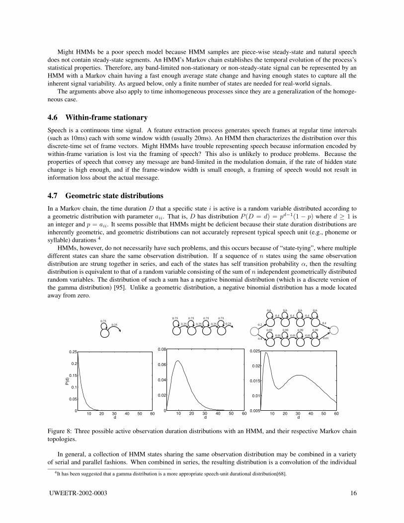
4.7 Geometric state distributionsIn a Markov chain, the time duration D that a specific state i is active is a random variable distributed according toa geometric distribution with parameter aii. That is, D has distribution P (D = d) = pd−1(1 − p) where d ≥ 1 isan integer and p = aii. It seems possible that HMMs might be deficient because their state duration distributions areinherently geometric, and geometric distributions can not accurately represent typical speech unit (e.g., phoneme orsyllable) durations 4

HMMs, however, do not necessarily have such problems, and this occurs because of “state-tying”, where multipledifferent states can share the same observation distribution. If a sequence of n states using the same observationdistribution are strung together in series, and each of the states has self transition probability α, then the resultingdistribution is equivalent to that of a random variable consisting of the sum of n independent geometrically distributedrandom variables. The distribution of such a sum has a negative binomial distribution (which is a discrete version ofthe gamma distribution) [95]. Unlike a geometric distribution, a negative binomial distribution has a mode locatedaway from zero.

0.250.75

10 20 30 40 50 600

0.05

0.1

0.15

0.2

0.25

d

P(d

)

0.75

0.25

0.75

0.25

0.75

0.25

0.75

0.25

10 20 30 40 50 600

0.02

0.04

0.06

0.08

d

0.6

0.4

0.6

0.4

0.6

0.4

0.6

0.99

0.01

0.99

0.01

0.99

0.01

0.99

0.4

0.01

0.2

0.8

10 20 30 40 50 600.005

0.01

0.015

0.02

0.025

d

Figure 8: Three possible active observation duration distributions with an HMM, and their respective Markov chaintopologies.

In general, a collection of HMM states sharing the same observation distribution may be combined in a varietyof serial and parallel fashions. When combined in series, the resulting distribution is a convolution of the individual

4It has been suggested that a gamma distribution is a more appropriate speech-unit durational distribution[68].

UWEETR-2002-0003 16

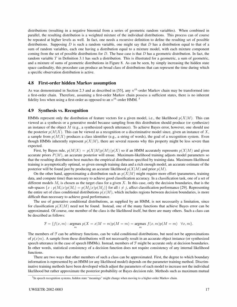
distributions (resulting in a negative binomial from a series of geometric random variables). When combined inparallel, the resulting distribution is a weighted mixture of the individual distributions. This process can of coursebe repeated at higher levels as well. In fact, one needs a recursive definition to define the resulting set of possibledistributions. Supposing D is such a random variable, one might say that D has a distribution equal to that of asum of random variables, each one having a distribution equal to a mixture model, with each mixture componentcoming from the set of possible distributions for D. The base case is that D has a geometric distribution. In fact, therandom variable T in Definition 3.1 has such a distribution. This is illustrated for a geometric, a sum of geometric,and a mixture of sums of geometric distributions in Figure 8. As can be seen, by simply increasing the hidden statespace cardinality, this procedure can produce an broad class of distributions that can represent the time during whicha specific observation distribution is active.

4.8 First-order hidden Markov assumptionAs was demonstrated in Section 2.3 and as described in [55], any nth-order Markov chain may be transformed intoa first-order chain. Therefore, assuming a first-order Markov chain possess a sufficient states, there is no inherentfidelity loss when using a first-order as opposed to an nth-order HMM. 5

4.9 Synthesis vs. RecognitionHMMs represent only the distribution of feature vectors for a given model, i.e., the likelihood p(X|M). This canviewed as a synthesis or a generative model because sampling from this distribution should produce (or synthesize)an instance of the object M (e.g., a synthesized speech utterance). To achieve Bayes error, however, one should usethe posterior p(M |X). This can be viewed as a recognition or a discriminative model since, given an instance of X ,a sample from p(M |X) produces a class identifier (e.g., a string of words), the goal of a recognition system. Eventhough HMMs inherently represent p(X|M), there are several reasons why this property might be less severe thanexpected.

First, by Bayes rule, p(M |X) = p(X|M)p(M)/p(X) so if an HMM accurately represents p(X|M) and givenaccurate priors P (M), an accurate posterior will ensue. Maximum-likelihood training adjusts model parameters sothat the resulting distribution best matches the empirical distribution specified by training-data. Maximum-likelihoodtraining is asymptotically optimal, so given enough training data and a rich enough model, an accurate estimate of theposterior will be found just by producing an accurate likelihood p(X|M) and prior p(M).

On the other hand, approximating a distribution such as p(X|M) might require more effort (parameters, trainingdata, and compute time) than necessary to achieve good classification accuracy. In a classification task, one of a set ofdifferent models Mi is chosen as the target class for a given X . In this case, only the decision boundaries, that is thesub-spaces {x : p(Mi|x)p(Mi) = p(Mj |x)p(Mj)} for all i 6= j, affect classification performance [29]. Representingthe entire set of class conditional distributions p(x|M), which includes regions between decision boundaries, is moredifficult than necessary to achieve good performance.

The use of generative conditional distributions, as supplied by an HMM, is not necessarily a limitation, sincefor classification p(X|M) need not be found. Instead, one of the many functions that achieve Bayes error can beapproximated. Of course, one member of the class is the likelihood itself, but there are many others. Such a class canbe described as follows:

F = {f(x,m) : argmaxm

p(X = x|M = m)p(M = m) = argmaxm

f(x,m)p(M = m) ∀x,m}.

The members of F can be arbitrary functions, can be valid conditional distributions, but need not be approximationsof p(x|m). A sample from these distributions will not necessarily result in an accurate object instance (or synthesizedspeech utterance in the case of speech HMMs). Instead, members of F might be accurate only at decision boundaries.In other words, statistical consistency of a decision function does not require consistency of any internal likelihoodfunctions.

There are two ways that other members of such a class can be approximated. First, the degree to which boundaryinformation is represented by an HMM (or any likelihood model) depends on the parameter training method. Discrim-inative training methods have been developed which adjust the parameters of each model to increase not the individuallikelihood but rather approximate the posterior probability or Bayes decision rule. Methods such as maximum mutual

5In speech recognition systems, hidden state “meanings” might change when moving to a higher-order Markov chain.

UWEETR-2002-0003 17

information (MMI) [1, 13], minimum discrimination information (MDI) [32, 33], minimum classification error (MCE)[59, 58], and more generally risk minimization [29, 97] essentially attempt to optimize p(M |X) by adjusting whatevermodel parameters are available, be they the likelihoods p(X|M), posteriors, or something else.

Second, the degree to which boundary information is represented depends on each model’s intrinsic ability toproduce a probability distribution at decision boundaries vs. its ability to produce a distribution between boundaries.This is the inherent discriminability of the structure of the model for each class, independent of its parameters. Modelswith this property have been called structurally discriminative [8].

Objects of class A Objects of class B

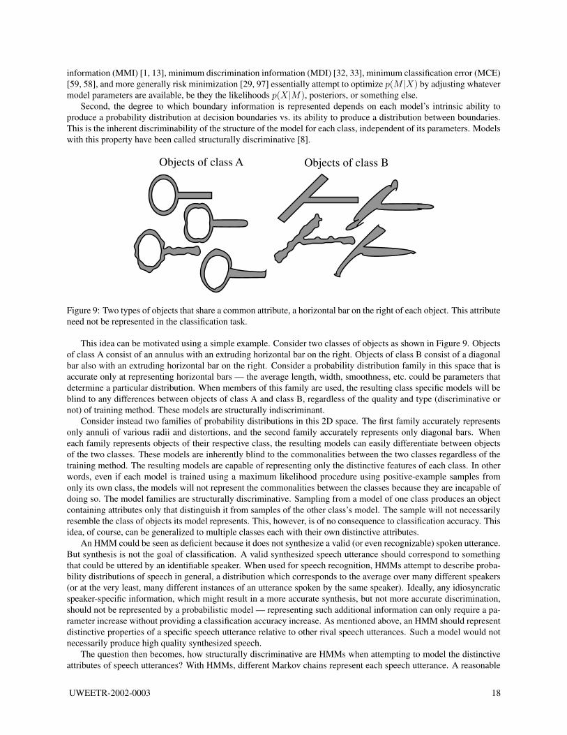
Figure 9: Two types of objects that share a common attribute, a horizontal bar on the right of each object. This attributeneed not be represented in the classification task.

This idea can be motivated using a simple example. Consider two classes of objects as shown in Figure 9. Objectsof class A consist of an annulus with an extruding horizontal bar on the right. Objects of class B consist of a diagonalbar also with an extruding horizontal bar on the right. Consider a probability distribution family in this space that isaccurate only at representing horizontal bars — the average length, width, smoothness, etc. could be parameters thatdetermine a particular distribution. When members of this family are used, the resulting class specific models will beblind to any differences between objects of class A and class B, regardless of the quality and type (discriminative ornot) of training method. These models are structurally indiscriminant.

Consider instead two families of probability distributions in this 2D space. The first family accurately representsonly annuli of various radii and distortions, and the second family accurately represents only diagonal bars. Wheneach family represents objects of their respective class, the resulting models can easily differentiate between objectsof the two classes. These models are inherently blind to the commonalities between the two classes regardless of thetraining method. The resulting models are capable of representing only the distinctive features of each class. In otherwords, even if each model is trained using a maximum likelihood procedure using positive-example samples fromonly its own class, the models will not represent the commonalities between the classes because they are incapable ofdoing so. The model families are structurally discriminative. Sampling from a model of one class produces an objectcontaining attributes only that distinguish it from samples of the other class’s model. The sample will not necessarilyresemble the class of objects its model represents. This, however, is of no consequence to classification accuracy. Thisidea, of course, can be generalized to multiple classes each with their own distinctive attributes.

An HMM could be seen as deficient because it does not synthesize a valid (or even recognizable) spoken utterance.But synthesis is not the goal of classification. A valid synthesized speech utterance should correspond to somethingthat could be uttered by an identifiable speaker. When used for speech recognition, HMMs attempt to describe proba-bility distributions of speech in general, a distribution which corresponds to the average over many different speakers(or at the very least, many different instances of an utterance spoken by the same speaker). Ideally, any idiosyncraticspeaker-specific information, which might result in a more accurate synthesis, but not more accurate discrimination,should not be represented by a probabilistic model — representing such additional information can only require a pa-rameter increase without providing a classification accuracy increase. As mentioned above, an HMM should representdistinctive properties of a specific speech utterance relative to other rival speech utterances. Such a model would notnecessarily produce high quality synthesized speech.

The question then becomes, how structurally discriminative are HMMs when attempting to model the distinctiveattributes of speech utterances? With HMMs, different Markov chains represent each speech utterance. A reasonable

UWEETR-2002-0003 18

assumption is that HMMs are not structurally indiscriminant because, even when trained using a simple maximumlikelihood procedure, HMM-based speech recognition systems perform reasonably well. Sampling from such anHMM might produce an unrealistic speech utterance, but the underlying distribution might be accurate at decisionboundaries. Such an approach was taken in [8], where HMM dependencies were augmented to increase structuraldiscriminability.

Earlier sections of this paper suggested that HMM distributions are not destitute in their flexibility, but this sectionclaimed that for the recognition task an HMM need not accurately represent the true likelihood p(X|M) to achievehigh classification accuracy. While HMMs are powerful, a fortunate consequence of the above discussion is thatHMMs need not capture many nuances in a speech signal and may be simpler as a result. In any event, just because aparticular HMM does not represent speech utterances does not mean it is poor at the recognition task.

5 Conditions for HMM AccuracySuppose that p(X1:T ) is the true distribution of the observation variables X1:T . In this section, it is shown that if anHMM represents this distribution accurately, necessary conditions on the number of hidden states and the necessarycomplexity of the observation distributions may be found. Let ph(X1:T ) be the joint distribution over the observationvariables under an HMM. HMM accuracy is defined as KL-distance between the two distributions being zero, i.e.:

D(p(X1:T )||ph(X1:T )) = 0

If this condition is true, the mutual information between any subset of variables under each distribution will be equal.That is,

I(XS1;XS2

) = Ih(XS1;XS2

)

where I(·; ·) is the mutual information between two random vectors under the true distribution, Ih(·; ·) is the mutualinformation under the HMM, and Si is any subset of 1:T .

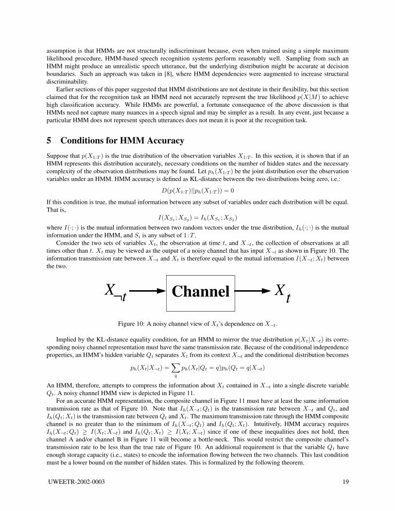
Consider the two sets of variables Xt, the observation at time t, and X¬t, the collection of observations at alltimes other than t. Xt may be viewed as the output of a noisy channel that has input X¬t as shown in Figure 10. Theinformation transmission rate between X¬t and Xt is therefore equal to the mutual information I(X¬t;Xt) betweenthe two.

X XtChannelt ¬

Figure 10: A noisy channel view of Xt’s dependence on X¬t.

Implied by the KL-distance equality condition, for an HMM to mirror the true distribution p(Xt|X¬t) its corre-sponding noisy channel representation must have the same transmission rate. Because of the conditional independenceproperties, an HMM’s hidden variable Qt separates Xt from its context X¬t and the conditional distribution becomes

ph(Xt|X¬t) =∑

q

ph(Xt|Qt = q)ph(Qt = q|X¬t)

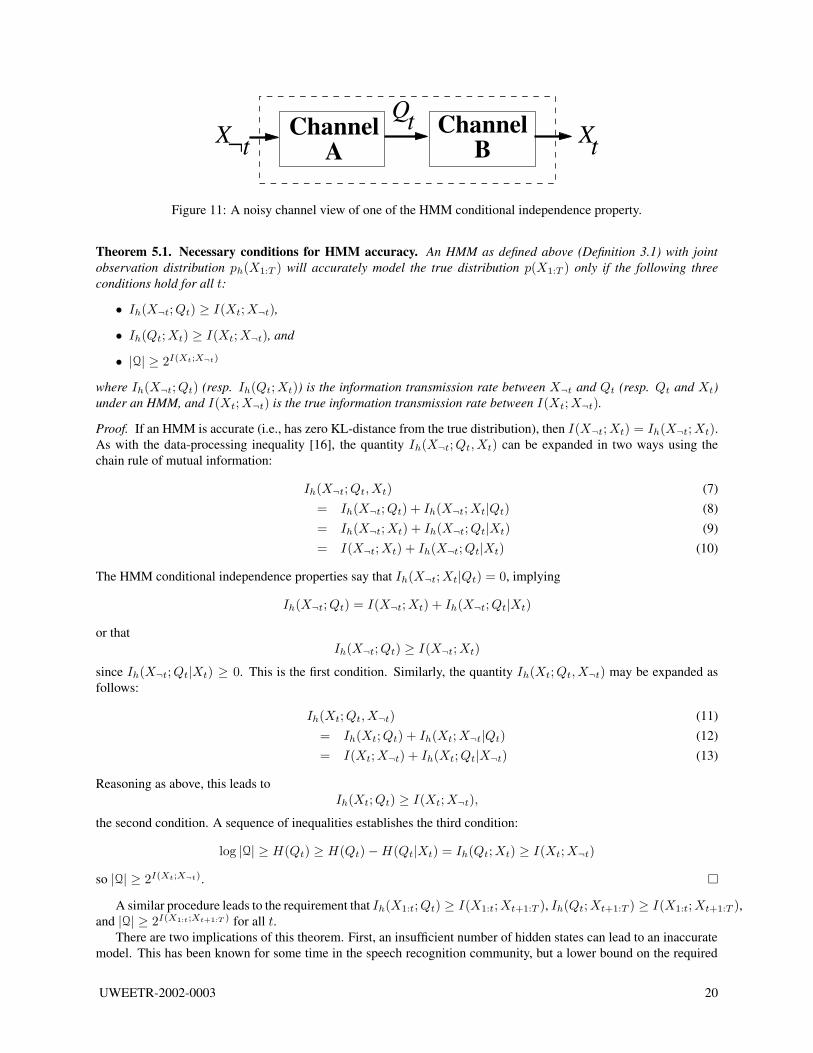
An HMM, therefore, attempts to compress the information about Xt contained in X¬t into a single discrete variableQt. A noisy channel HMM view is depicted in Figure 11.

For an accurate HMM representation, the composite channel in Figure 11 must have at least the same informationtransmission rate as that of Figure 10. Note that Ih(X¬t;Qt) is the transmission rate between X¬t and Qt, andIh(Qt;Xt) is the transmission rate between Qt and Xt. The maximum transmission rate through the HMM compositechannel is no greater than to the minimum of Ih(X¬t;Qt) and Ih(Qt;Xt). Intuitively, HMM accuracy requiresIh(X¬t;Qt) ≥ I(Xt;X¬t) and Ih(Qt;Xt) ≥ I(Xt;X¬t) since if one of these inequalities does not hold, thenchannel A and/or channel B in Figure 11 will become a bottle-neck. This would restrict the composite channel’stransmission rate to be less than the true rate of Figure 10. An additional requirement is that the variable Qt haveenough storage capacity (i.e., states) to encode the information flowing between the two channels. This last conditionmust be a lower bound on the number of hidden states. This is formalized by the following theorem.

UWEETR-2002-0003 19

X XtQtChannel Channel

A Bt¬

Figure 11: A noisy channel view of one of the HMM conditional independence property.

Theorem 5.1. Necessary conditions for HMM accuracy. An HMM as defined above (Definition 3.1) with jointobservation distribution ph(X1:T ) will accurately model the true distribution p(X1:T ) only if the following threeconditions hold for all t:

• Ih(X¬t;Qt) ≥ I(Xt;X¬t),

• Ih(Qt;Xt) ≥ I(Xt;X¬t), and

• |Q| ≥ 2I(Xt;X¬t)

where Ih(X¬t;Qt) (resp. Ih(Qt;Xt)) is the information transmission rate between X¬t and Qt (resp. Qt and Xt)under an HMM, and I(Xt;X¬t) is the true information transmission rate between I(Xt;X¬t).

Proof. If an HMM is accurate (i.e., has zero KL-distance from the true distribution), then I(X¬t;Xt) = Ih(X¬t;Xt).As with the data-processing inequality [16], the quantity Ih(X¬t;Qt, Xt) can be expanded in two ways using thechain rule of mutual information:

Ih(X¬t;Qt, Xt) (7)= Ih(X¬t;Qt) + Ih(X¬t;Xt|Qt) (8)= Ih(X¬t;Xt) + Ih(X¬t;Qt|Xt) (9)= I(X¬t;Xt) + Ih(X¬t;Qt|Xt) (10)

The HMM conditional independence properties say that Ih(X¬t;Xt|Qt) = 0, implying

Ih(X¬t;Qt) = I(X¬t;Xt) + Ih(X¬t;Qt|Xt)

or thatIh(X¬t;Qt) ≥ I(X¬t;Xt)

since Ih(X¬t;Qt|Xt) ≥ 0. This is the first condition. Similarly, the quantity Ih(Xt;Qt, X¬t) may be expanded asfollows:

Ih(Xt;Qt, X¬t) (11)= Ih(Xt;Qt) + Ih(Xt;X¬t|Qt) (12)= I(Xt;X¬t) + Ih(Xt;Qt|X¬t) (13)

Reasoning as above, this leads toIh(Xt;Qt) ≥ I(Xt;X¬t),

the second condition. A sequence of inequalities establishes the third condition:

log |Q| ≥ H(Qt) ≥ H(Qt) − H(Qt|Xt) = Ih(Qt;Xt) ≥ I(Xt;X¬t)

so |Q| ≥ 2I(Xt;X¬t).

A similar procedure leads to the requirement that Ih(X1:t;Qt) ≥ I(X1:t;Xt+1:T ), Ih(Qt;Xt+1:T ) ≥ I(X1:t;Xt+1:T ),and |Q| ≥ 2I(X1:t;Xt+1:T ) for all t.

There are two implications of this theorem. First, an insufficient number of hidden states can lead to an inaccuratemodel. This has been known for some time in the speech recognition community, but a lower bound on the required

UWEETR-2002-0003 20

number of states has not been established. With an HMM, the information about Xt contained in X<t is squeezedthrough the hidden state variable Qt. Depending on the number of hidden states, this can overburden Qt and result inan inaccurate probabilistic model. But if there are enough states, and if the information in the surrounding acousticcontext is appropriately encoded in the hidden states, the required information may be compressed and representedby Qt. An appropriate encoding of the contextual information is essential since just adding states does not guaranteeaccuracy will increase.

To achieve high accuracy, it is likely that a finite number of states is required for any real task since signalsrepresenting natural objects will have bounded mutual information. Recall that the first order Markov assumption inthe hidden Markov chain is not necessarily a problem since a first-order chain may represent an nth order chain (seeSection 2.3 and [55]).

The second implication of this theorem is that each of the two channels in Figure 11 must be sufficiently powerful.HMM inaccuracy can result from using a poor observation distribution family which corresponds to using a channelwith too small a capacity. The capacity of an observation distribution is, for example, determined by the number ofGaussian components or covariance type in a Gaussian mixture HMM [107], or the number of hidden units in anHMM with MLP [9] observation distributions [11, 75].

In any event, just increasing the number of components in a Gaussian mixture system or increasing the numberof hidden units in an MLP system does not necessarily improve HMM accuracy because the bottle-neck ultimatelybecomes the fixed number of hidden states (i.e., value of |Q|). Alternatively, simply increasing the number of HMMhidden states might not increase accuracy if the observation model is too weak. Of course, any increase in the numberof model parameters must accompany a training data increase to yield reliable low-variance parameter estimates.

Can sufficient conditions for HMM accuracy be found? Assume for the moment that Xt is a discrete randomvariable with finite cardinality. Recall that X<t

∆= X1:t−1. Suppose that Hh(Qt|X<t) = 0 for all t (a worst case

HMM condition to achieve this property is when every observation sequence has its own unique Markov chain stateassignment). This implies that Qt is a deterministic function of X<t (i.e., Qt = f(X<t) for some f(·)). Consider theHMM approximation:

ph(xt|x<t) =∑

qt

ph(xt|qt)ph(qt|x<t) (14)

but because H(Qt|X<t) = 0, the approximation becomes

ph(xt|x<t) = ph(xt|qx<t)

where qx<t= f(x<t) since every other term in the sum in Equation 14 is zero. The variable Xt is discrete, so for

each value of xt and for each hidden state assignment qx<t, the distribution ph(Xt = xt|qx<t

) can be set as follows:

ph(Xt = xt|qx<t) = p(Xt = xt|X<t = x<t)

This last condition might require a number of hidden states equal to the cardinality of the discrete observation space,i.e., |X1:T | which can be very large. In any event, it follows that for all t:

D(p(Xt|X<t)||ph(Xt|X<t))

=∑

x1:t

p(x1:t) logp(xt|x<t)

ph(xt|x<t)

=∑

x1:t

p(x1:t) logp(xt|x<t)

∑

qtph(xt|qt)ph(qt|x<t)

=∑

x1:t

p(x1:t) logp(xt|x<t)

ph(xt|qx<t)

=∑

x1:t

p(x1:t) logp(xt|x<t)

p(xt|x<t)

= 0

UWEETR-2002-0003 21

It then follows, using the above equation, that:

0 =∑

t

D(p(Xt|X<t)||ph(Xt|X<t))

=∑

t

∑

x1:t

p(x1:t) logp(xt|x<t)

ph(xt|x<t)

=∑

t

∑

x1:T

p(x1:T ) logp(xt|x<t)

ph(xt|x<t)

=∑

x1:T

p(x1:T ) log

∏

t p(xt|x<t)∏

t ph(xt|x<t)

=∑

x1:T

p(x1:T ) logp(x1:T )

ph(x1:T )

= D(p(X1:T )||ph(X1:T ))

In other words, the HMM is a perfect representation of the true distribution, proving the following theorem.

Theorem 5.2. Sufficient conditions for HMM accuracy. An HMM as defined above (Definition 3.1) with a jointdiscrete distribution ph(X1:T ) will accurately represent a true discrete distribution p(X1:T ) if the following conditionshold for all t:

• H(Qt|X<t) = 0

• ph(Xt = xt|qx<t) = p(Xt = xt|X<t = x<t).

It remains to be seen if simultaneously necessary and sufficient conditions can be derived to achieve HMM accu-racy, if it is possible to derive sufficient conditions for continuous observation vector HMMs under some reasonableconditions (e.g., finite power, etc.), and what conditions might exist for an HMM that is allowed to have a fixedupper-bound KL-distance error.

6 What HMMs Can’t DoFrom the previous sections, there appears to be little an HMM can’t do. If under the true probability distribution,two random variables possess extremely large mutual information, an HMM approximation might fail because of therequired number of states required. This is unlikely, however, for distributions representing objects contained in thenatural world.

One problem with HMMs is how they are used; the conditional independence properties are inaccurate when thereare too few hidden states, or when the observation distributions are inadequate. Moreover, a demonstration of HMMgenerality acquaints us not with other inherently more parsimonious models which could be superior. This is exploredin the next section.

6.1 How to Improve an HMMThe conceptually easiest way to increase an HMM’s accuracy is by increasing the number of hidden states and thecapacity of the observation distributions. Indeed, this approach is very effective. In speech recognition systems, it iscommon to use multiple states per phoneme and to use collections of states corresponding to tri-phones, quad-phones,or even penta-phones. State-of-the-art speech recognition systems have achieved their performance on difficult speechcorpora partially by increasing the number of hidden states. For example, in the 1999 DARPA Broadcast NewsWorkshop [19], the best performing systems used penta-phones (a phoneme in the context of two preceding and twosucceeding phonemes) and multiple hidden states for each penta-phone. At the time of this writing, some advancedsystems condition on both the preceding and succeeding five phonemes leading to what could be called “unodeca-phones.” Given limits of training data size, such systems must use methods to reduce what otherwise would be anenormous number of parameters — this is done by automatically tying parameters of different states together [107].

UWEETR-2002-0003 22

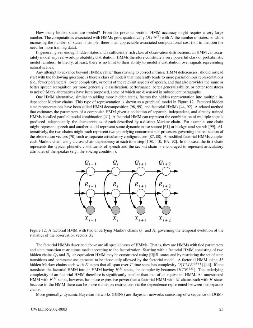
How many hidden states are needed? From the previous section, HMM accuracy might require a very largenumber. The computations associated with HMMs grow quadratically O(TN 2) with N the number of states, so whileincreasing the number of states is simple, there is an appreciable associated computational cost (not to mention theneed for more training data).

In general, given enough hidden states and a sufficiently rich class of observation distributions, an HMM can accu-rately model any real-world probability distribution. HMMs therefore constitute a very powerful class of probabilisticmodel families. In theory, at least, there is no limit to their ability to model a distribution over signals representingnatural scenes.

Any attempt to advance beyond HMMs, rather than striving to correct intrinsic HMM deficiencies, should insteadstart with the following question: is there a class of models that inherently leads to more parsimonious representations(i.e., fewer parameters, lower complexity, or both) of the relevant aspects of speech, and that also provides the same orbetter speech recognition (or more generally, classification) performance, better generalizability, or better robustnessto noise? Many alternatives have been proposed, some of which are discussed in subsequent paragraphs.

One HMM alternative, similar to adding more hidden states, factors the hidden representation into multiple in-dependent Markov chains. This type of representation is shown as a graphical model in Figure 12. Factored hiddenstate representations have been called HMM decomposition [98, 99], and factorial HMMs [44, 92]. A related methodthat estimates the parameters of a composite HMM given a collection of separate, independent, and already trainedHMMs is called parallel model combination [41]. A factorial HMM can represent the combination of multiple signalsproduced independently, the characteristics of each described by a distinct Markov chain. For example, one chainmight represent speech and another could represent some dynamic noise source [61] or background speech [99]. Al-ternatively, the two chains might each represent two underlying concurrent sub-processes governing the realization ofthe observation vectors [70] such as separate articulatory configurations [87, 88]. A modified factorial HMMs coupleseach Markov chain using a cross-chain dependency at each time step [108, 110, 109, 92]. In this case, the first chainrepresents the typical phonetic constituents of speech and the second chain is encouraged to represent articulatoryattributes of the speaker (e.g., the voicing condition).

R t R t 1+R t 1– R t 2+

Qt Qt 1+Qt 1– Qt 2+

X t X t 1+X t 1– X t 2+

Figure 12: A factorial HMM with two underlying Markov chains Qt and Rt governing the temporal evolution of thestatistics of the observation vectors Xt.

The factorial HMMs described above are all special cases of HMMs. That is, they are HMMs with tied parametersand state transition restrictions made according to the factorization. Starting with a factorial HMM consisting of twohidden chains Qt and Rt, an equivalent HMM may be constructed using |Q||R| states and by restricting the set of statetransitions and parameter assignments to be those only allowed by the factorial model. A factorial HMM using Mhidden Markov chains each with K states that all span over T time steps has complexity O(TMKM+1) [44]. If onetranslates the factorial HMM into an HMM having KM states, the complexity becomes O(TK2M ). The underlyingcomplexity of an factorial HMM therefore is significantly smaller than that of an equivalent HMM. An unrestrictedHMM with KM states, however, has more expressive power than a factorial HMM with M chains each with K statesbecause in the HMM there can be more transition restrictions via the dependence represented between the separatechains.

More generally, dynamic Bayesian networks (DBNs) are Bayesian networks consisting of a sequence of DGMs

UWEETR-2002-0003 23

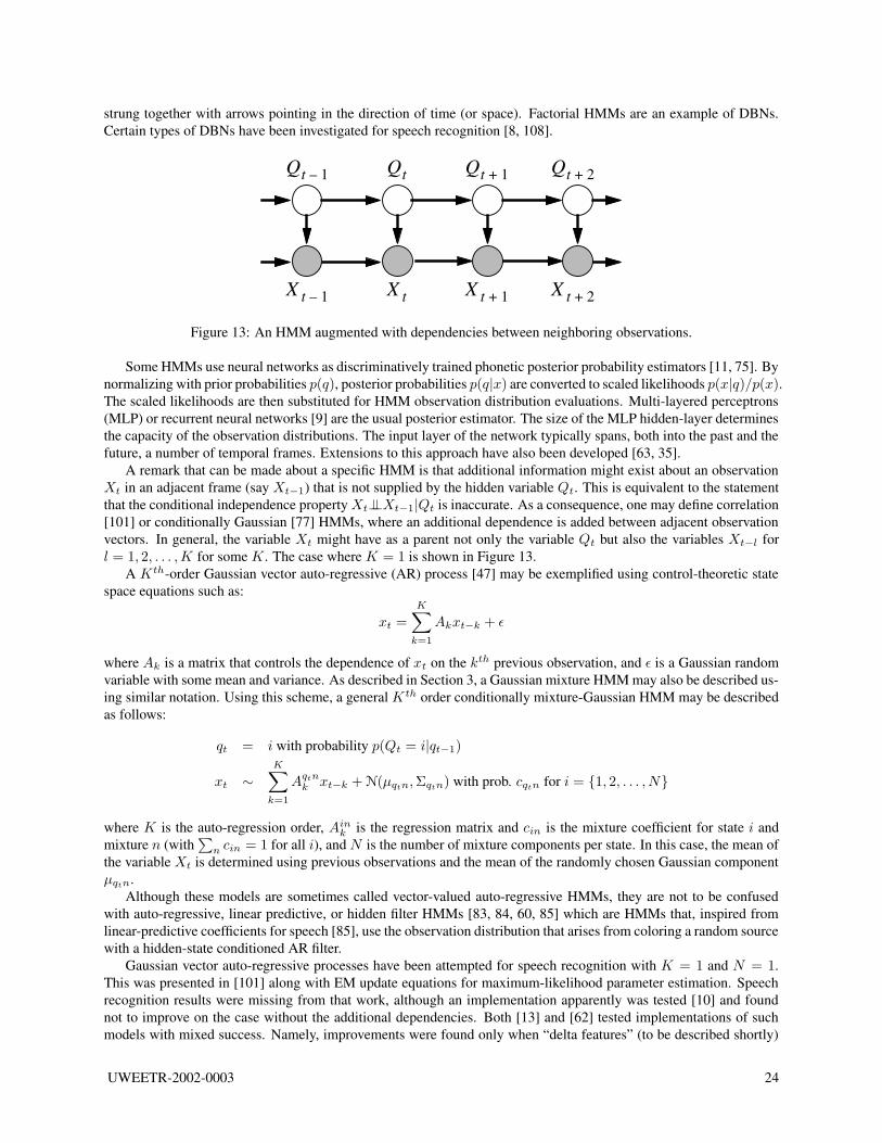
strung together with arrows pointing in the direction of time (or space). Factorial HMMs are an example of DBNs.Certain types of DBNs have been investigated for speech recognition [8, 108].

Qt Qt 1+Qt 1– Qt 2+

X t X t 1+X t 1– X t 2+

Figure 13: An HMM augmented with dependencies between neighboring observations.

Some HMMs use neural networks as discriminatively trained phonetic posterior probability estimators [11, 75]. Bynormalizing with prior probabilities p(q), posterior probabilities p(q|x) are converted to scaled likelihoods p(x|q)/p(x).The scaled likelihoods are then substituted for HMM observation distribution evaluations. Multi-layered perceptrons(MLP) or recurrent neural networks [9] are the usual posterior estimator. The size of the MLP hidden-layer determinesthe capacity of the observation distributions. The input layer of the network typically spans, both into the past and thefuture, a number of temporal frames. Extensions to this approach have also been developed [63, 35].

A remark that can be made about a specific HMM is that additional information might exist about an observationXt in an adjacent frame (say Xt−1) that is not supplied by the hidden variable Qt. This is equivalent to the statementthat the conditional independence property Xt⊥⊥Xt−1|Qt is inaccurate. As a consequence, one may define correlation[101] or conditionally Gaussian [77] HMMs, where an additional dependence is added between adjacent observationvectors. In general, the variable Xt might have as a parent not only the variable Qt but also the variables Xt−l forl = 1, 2, . . . ,K for some K. The case where K = 1 is shown in Figure 13.

A Kth-order Gaussian vector auto-regressive (AR) process [47] may be exemplified using control-theoretic statespace equations such as:

xt =

K∑

k=1

Akxt−k + ε

where Ak is a matrix that controls the dependence of xt on the kth previous observation, and ε is a Gaussian randomvariable with some mean and variance. As described in Section 3, a Gaussian mixture HMM may also be described us-ing similar notation. Using this scheme, a general K th order conditionally mixture-Gaussian HMM may be describedas follows:

qt = i with probability p(Qt = i|qt−1)

xt ∼

K∑

k=1

Aqtnk xt−k + N(µqtn,Σqtn) with prob. cqtn for i = {1, 2, . . . , N}

where K is the auto-regression order, Aink is the regression matrix and cin is the mixture coefficient for state i and

mixture n (with∑

n cin = 1 for all i), and N is the number of mixture components per state. In this case, the mean ofthe variable Xt is determined using previous observations and the mean of the randomly chosen Gaussian componentµqtn.

Although these models are sometimes called vector-valued auto-regressive HMMs, they are not to be confusedwith auto-regressive, linear predictive, or hidden filter HMMs [83, 84, 60, 85] which are HMMs that, inspired fromlinear-predictive coefficients for speech [85], use the observation distribution that arises from coloring a random sourcewith a hidden-state conditioned AR filter.

Gaussian vector auto-regressive processes have been attempted for speech recognition with K = 1 and N = 1.This was presented in [101] along with EM update equations for maximum-likelihood parameter estimation. Speechrecognition results were missing from that work, although an implementation apparently was tested [10] and foundnot to improve on the case without the additional dependencies. Both [13] and [62] tested implementations of suchmodels with mixed success. Namely, improvements were found only when “delta features” (to be described shortly)

UWEETR-2002-0003 24

were excluded. Similar results were found by [25] but for segment models (also described below). In [79], thedependency structure in Figure 13 used discrete rather than Gaussian observation densities. And in [76], a parallelalgorithm was presented that can efficiently perform inference with such models.

The use of dynamic or delta features [31, 37, 38, 39] has become standard in state-of-the-art speech recognitionsystems. While incorporating delta features does not correspond to a new model per se, they can also be viewed as anHMM model augmentation. Similar to conditionally Gaussian HMMs, dynamic features also represent dependenciesin the feature streams. Such information is gathered by computing an estimate of the time derivative of each featureddtXt = Xt and then augmenting the feature stream with those estimates, i.e., X ′

t = {Xt,ddtXt}. Acceleration, or

delta-delta, features are defined similarly and are sometimes found to be additionally beneficial [104, 65].Most often, estimates of the feature derivative are obtained [85] using linear regression, i.e.,

xt =

K∑

k=−K

kxt

K∑

k=−K

k2

where K is the number of points to fit the regression. Delta (or delta-delta) features are therefore similar to auto-regression, but where the regression is over samples not just from the past but also from the future. That is, consider ahypothetical process defined by

xt =

K∑

k=−K

akxt−k + ε

where the fixed regression coefficients ak are defined by ak = −k/∑K

l=−K l2 for k 6= 0 and a0 = 1. This isequivalent to

xt −

K∑

k=−K

akxt−k =

∑Kk=−K kxt−k∑K

l=−K l2= ε

which is the same as modeling delta features with a single Gaussian component.The addition of delta features to a feature stream is therefore similar to additionally using a separate conditionally

Gaussian observation model. Observing the HMM DGM (Figure 5), delta features add dependencies between obser-vation nodes and their neighbors from both the past and the future (the maximum range determined by K). Of course,this would create a directed cycle in a DGM violating its semantics. To be theoretically accurate, one must perform aglobal re-normalization as is done with a Markov random field [23]. Nevertheless, it can be seen that the use of deltafeatures corresponds in some sense to a relaxation of the HMM conditional independence properties.

As mentioned above, conditionally Gaussian HMMs often do not supply an improvement when delta features areincluded in the feature stream. Improvements were reported with delta features in [106] using discriminative outputdistributions [105]. In [66, 67], successful results were obtained using delta features but where the conditional mean,rather than being linear, was non-linear and was implemented using a neural network. Also, in [96], benefits wereobtained using mixtures of discrete distributions. In a similar model, improvements when using delta features werealso reported when sparse dependencies were chosen individually between feature vector elements, and according toan data-driven hidden-variable dependent information-theoretic criteria [8, 7, 5].

In general, one can consider the model

qt = i with prob. p(Qt = i|qt−1)

xt = Ft(xt−1, xt−1, . . . , xt−k)

where Ft is an arbitrary random function of the previous k observations. In [21, 22], the model becomes

xt =

K∑

k=1

φqt,t,kxt−k + gqt,t + εqt

where φi,t,k is a dependency matrix for state i and time lag k and is a polynomial function of t, gi,t is a fixed mean forstate i and time t, and εi is a state dependent Gaussian. Improvements using this model were also found with featurestreams that included delta features.

UWEETR-2002-0003 25

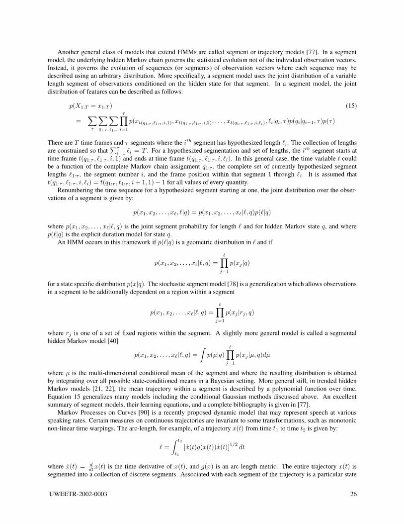
Another general class of models that extend HMMs are called segment or trajectory models [77]. In a segmentmodel, the underlying hidden Markov chain governs the statistical evolution not of the individual observation vectors.Instead, it governs the evolution of sequences (or segments) of observation vectors where each sequence may bedescribed using an arbitrary distribution. More specifically, a segment model uses the joint distribution of a variablelength segment of observations conditioned on the hidden state for that segment. In a segment model, the jointdistribution of features can be described as follows:

p(X1:T = x1:T ) (15)

=∑

τ

∑

q1:τ

∑

`1:τ

τ∏

i=1

p(xt(q1:τ ,`1:τ ,i,1), xt(q1:τ ,`1:τ ,i,2), . . . , xt(q1:τ ,`1:τ ,i,`i), `i|qi, τ)p(qi|qi−1, τ)p(τ)

There are T time frames and τ segments where the ith segment has hypothesized length `i. The collection of lengthsare constrained so that

∑τi=1 `i = T . For a hypothesized segmentation and set of lengths, the ith segment starts at

time frame t(q1:τ , `1:τ , i, 1) and ends at time frame t(q1:τ , `1:τ , i, `i). In this general case, the time variable t couldbe a function of the complete Markov chain assignment q1:τ , the complete set of currently hypothesized segmentlengths `1:τ , the segment number i, and the frame position within that segment 1 through `i. It is assumed thatt(q1:τ , `1:τ , i, `i) = t(q1:τ , `1:τ , i + 1, 1) − 1 for all values of every quantity.

Renumbering the time sequence for a hypothesized segment starting at one, the joint distribution over the obser-vations of a segment is given by:

p(x1, x2, . . . , x`, `|q) = p(x1, x2, . . . , x`|`, q)p(`|q)

where p(x1, x2, . . . , x`|`, q) is the joint segment probability for length ` and for hidden Markov state q, and wherep(`|q) is the explicit duration model for state q.

An HMM occurs in this framework if p(`|q) is a geometric distribution in ` and if

p(x1, x2, . . . , x`|`, q) =∏

j=1

p(xj |q)

for a state specific distribution p(x|q). The stochastic segment model [78] is a generalization which allows observationsin a segment to be additionally dependent on a region within a segment

p(x1, x2, . . . , x`|`, q) =∏

j=1

p(xj |rj , q)

where rj is one of a set of fixed regions within the segment. A slightly more general model is called a segmentalhidden Markov model [40]

p(x1, x2, . . . , x`|`, q) =

∫

p(µ|q)∏

j=1

p(xj |µ, q)dµ

where µ is the multi-dimensional conditional mean of the segment and where the resulting distribution is obtainedby integrating over all possible state-conditioned means in a Bayesian setting. More general still, in trended hiddenMarkov models [21, 22], the mean trajectory within a segment is described by a polynomial function over time.Equation 15 generalizes many models including the conditional Gaussian methods discussed above. An excellentsummary of segment models, their learning equations, and a complete bibliography is given in [77].

Markov Processes on Curves [90] is a recently proposed dynamic model that may represent speech at variousspeaking rates. Certain measures on continuous trajectories are invariant to some transformations, such as monotonicnon-linear time warpings. The arc-length, for example, of a trajectory x(t) from time t1 to time t2 is given by:

` =

∫ t2

t1

[x(t)g(x(t))x(t)]1/2

dt

where x(t) = ddtx(t) is the time derivative of x(t), and g(x) is an arc-length metric. The entire trajectory x(t) is

segmented into a collection of discrete segments. Associated with each segment of the trajectory is a particular state

UWEETR-2002-0003 26

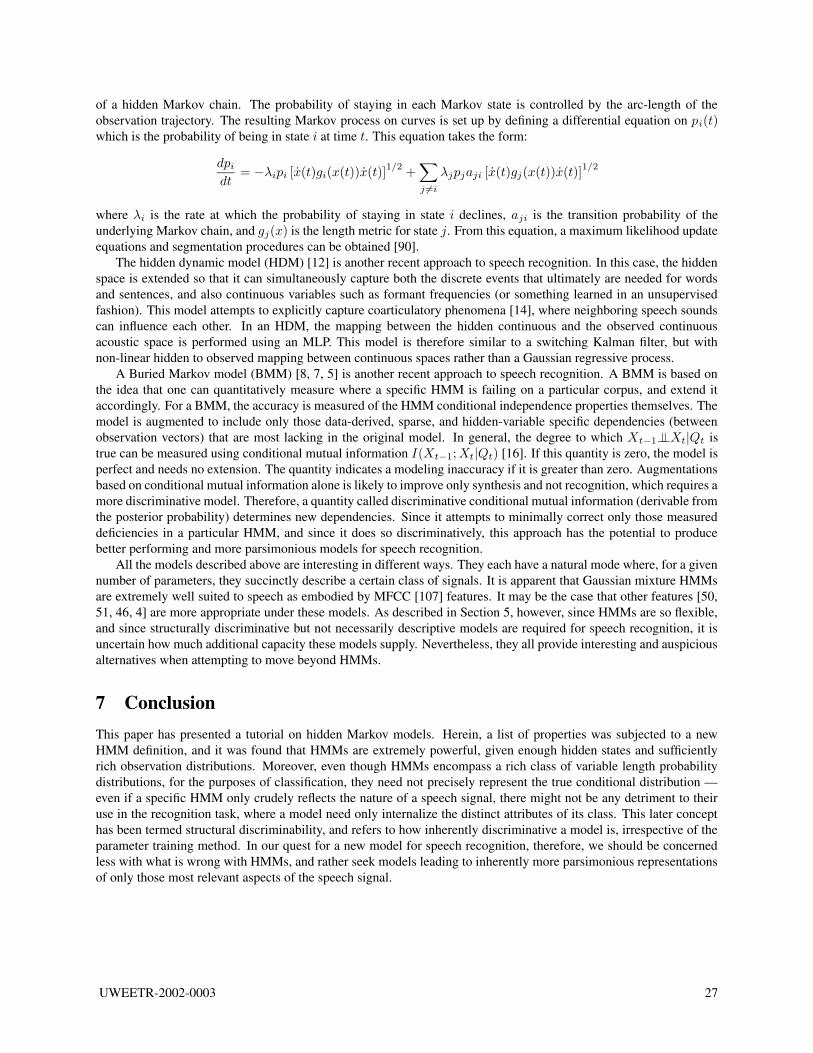
of a hidden Markov chain. The probability of staying in each Markov state is controlled by the arc-length of theobservation trajectory. The resulting Markov process on curves is set up by defining a differential equation on pi(t)which is the probability of being in state i at time t. This equation takes the form:

dpi

dt= −λipi [x(t)gi(x(t))x(t)]

1/2+∑

j 6=i

λjpjaji [x(t)gj(x(t))x(t)]1/2

where λi is the rate at which the probability of staying in state i declines, aji is the transition probability of theunderlying Markov chain, and gj(x) is the length metric for state j. From this equation, a maximum likelihood updateequations and segmentation procedures can be obtained [90].

The hidden dynamic model (HDM) [12] is another recent approach to speech recognition. In this case, the hiddenspace is extended so that it can simultaneously capture both the discrete events that ultimately are needed for wordsand sentences, and also continuous variables such as formant frequencies (or something learned in an unsupervisedfashion). This model attempts to explicitly capture coarticulatory phenomena [14], where neighboring speech soundscan influence each other. In an HDM, the mapping between the hidden continuous and the observed continuousacoustic space is performed using an MLP. This model is therefore similar to a switching Kalman filter, but withnon-linear hidden to observed mapping between continuous spaces rather than a Gaussian regressive process.

A Buried Markov model (BMM) [8, 7, 5] is another recent approach to speech recognition. A BMM is based onthe idea that one can quantitatively measure where a specific HMM is failing on a particular corpus, and extend itaccordingly. For a BMM, the accuracy is measured of the HMM conditional independence properties themselves. Themodel is augmented to include only those data-derived, sparse, and hidden-variable specific dependencies (betweenobservation vectors) that are most lacking in the original model. In general, the degree to which Xt−1⊥⊥Xt|Qt istrue can be measured using conditional mutual information I(Xt−1;Xt|Qt) [16]. If this quantity is zero, the model isperfect and needs no extension. The quantity indicates a modeling inaccuracy if it is greater than zero. Augmentationsbased on conditional mutual information alone is likely to improve only synthesis and not recognition, which requires amore discriminative model. Therefore, a quantity called discriminative conditional mutual information (derivable fromthe posterior probability) determines new dependencies. Since it attempts to minimally correct only those measureddeficiencies in a particular HMM, and since it does so discriminatively, this approach has the potential to producebetter performing and more parsimonious models for speech recognition.

All the models described above are interesting in different ways. They each have a natural mode where, for a givennumber of parameters, they succinctly describe a certain class of signals. It is apparent that Gaussian mixture HMMsare extremely well suited to speech as embodied by MFCC [107] features. It may be the case that other features [50,51, 46, 4] are more appropriate under these models. As described in Section 5, however, since HMMs are so flexible,and since structurally discriminative but not necessarily descriptive models are required for speech recognition, it isuncertain how much additional capacity these models supply. Nevertheless, they all provide interesting and auspiciousalternatives when attempting to move beyond HMMs.

7 ConclusionThis paper has presented a tutorial on hidden Markov models. Herein, a list of properties was subjected to a newHMM definition, and it was found that HMMs are extremely powerful, given enough hidden states and sufficientlyrich observation distributions. Moreover, even though HMMs encompass a rich class of variable length probabilitydistributions, for the purposes of classification, they need not precisely represent the true conditional distribution —even if a specific HMM only crudely reflects the nature of a speech signal, there might not be any detriment to theiruse in the recognition task, where a model need only internalize the distinct attributes of its class. This later concepthas been termed structural discriminability, and refers to how inherently discriminative a model is, irrespective of theparameter training method. In our quest for a new model for speech recognition, therefore, we should be concernedless with what is wrong with HMMs, and rather seek models leading to inherently more parsimonious representationsof only those most relevant aspects of the speech signal.

UWEETR-2002-0003 27

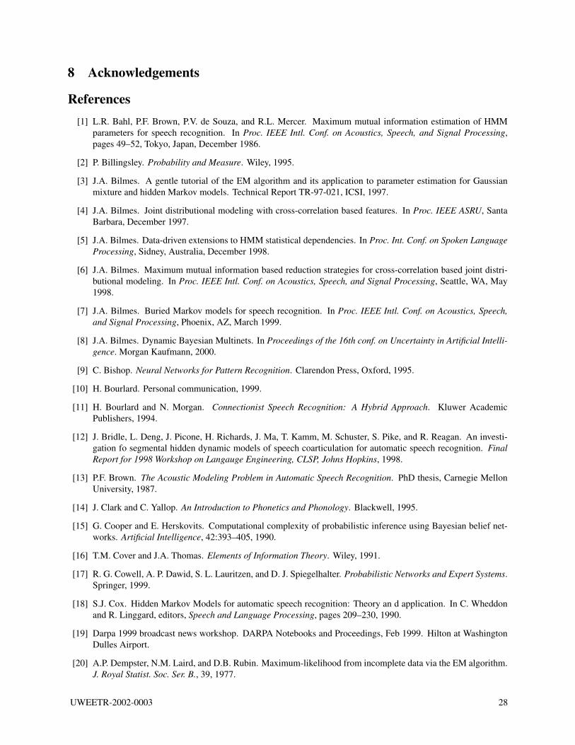
8 Acknowledgements

References[1] L.R. Bahl, P.F. Brown, P.V. de Souza, and R.L. Mercer. Maximum mutual information estimation of HMM

parameters for speech recognition. In Proc. IEEE Intl. Conf. on Acoustics, Speech, and Signal Processing,pages 49–52, Tokyo, Japan, December 1986.

[2] P. Billingsley. Probability and Measure. Wiley, 1995.

[3] J.A. Bilmes. A gentle tutorial of the EM algorithm and its application to parameter estimation for Gaussianmixture and hidden Markov models. Technical Report TR-97-021, ICSI, 1997.

[4] J.A. Bilmes. Joint distributional modeling with cross-correlation based features. In Proc. IEEE ASRU, SantaBarbara, December 1997.

[5] J.A. Bilmes. Data-driven extensions to HMM statistical dependencies. In Proc. Int. Conf. on Spoken LanguageProcessing, Sidney, Australia, December 1998.

[6] J.A. Bilmes. Maximum mutual information based reduction strategies for cross-correlation based joint distri-butional modeling. In Proc. IEEE Intl. Conf. on Acoustics, Speech, and Signal Processing, Seattle, WA, May1998.

[7] J.A. Bilmes. Buried Markov models for speech recognition. In Proc. IEEE Intl. Conf. on Acoustics, Speech,and Signal Processing, Phoenix, AZ, March 1999.

[8] J.A. Bilmes. Dynamic Bayesian Multinets. In Proceedings of the 16th conf. on Uncertainty in Artificial Intelli-gence. Morgan Kaufmann, 2000.

[9] C. Bishop. Neural Networks for Pattern Recognition. Clarendon Press, Oxford, 1995.

[10] H. Bourlard. Personal communication, 1999.

[11] H. Bourlard and N. Morgan. Connectionist Speech Recognition: A Hybrid Approach. Kluwer AcademicPublishers, 1994.

[12] J. Bridle, L. Deng, J. Picone, H. Richards, J. Ma, T. Kamm, M. Schuster, S. Pike, and R. Reagan. An investi-gation fo segmental hidden dynamic models of speech coarticulation for automatic speech recognition. FinalReport for 1998 Workshop on Langauge Engineering, CLSP, Johns Hopkins, 1998.

[13] P.F. Brown. The Acoustic Modeling Problem in Automatic Speech Recognition. PhD thesis, Carnegie MellonUniversity, 1987.

[14] J. Clark and C. Yallop. An Introduction to Phonetics and Phonology. Blackwell, 1995.

[15] G. Cooper and E. Herskovits. Computational complexity of probabilistic inference using Bayesian belief net-works. Artificial Intelligence, 42:393–405, 1990.

[16] T.M. Cover and J.A. Thomas. Elements of Information Theory. Wiley, 1991.

[17] R. G. Cowell, A. P. Dawid, S. L. Lauritzen, and D. J. Spiegelhalter. Probabilistic Networks and Expert Systems.Springer, 1999.

[18] S.J. Cox. Hidden Markov Models for automatic speech recognition: Theory an d application. In C. Wheddonand R. Linggard, editors, Speech and Language Processing, pages 209–230, 1990.

[19] Darpa 1999 broadcast news workshop. DARPA Notebooks and Proceedings, Feb 1999. Hilton at WashingtonDulles Airport.

[20] A.P. Dempster, N.M. Laird, and D.B. Rubin. Maximum-likelihood from incomplete data via the EM algorithm.J. Royal Statist. Soc. Ser. B., 39, 1977.

UWEETR-2002-0003 28

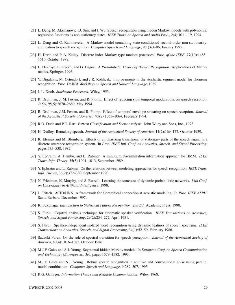
[21] L. Deng, M. Aksmanovic, D. Sun, and J. Wu. Speech recognition using hidden Markov models with polynomialregression functions as non-stationary states. IEEE Trans. on Speech and Audio Proc., 2(4):101–119, 1994.

[22] L. Deng and C. Rathinavelu. A Markov model containing state-conditioned second-order non-stationarity:application to speech recognition. Computer Speech and Language, 9(1):63–86, January 1995.

[23] H. Derin and P. A. Kelley. Discrete-index Markov-type random processes. Proc. of the IEEE, 77(10):1485–1510, October 1989.

[24] L. Devroye, L. Gyorfi, and G. Lugosi. A Probabilistic Theory of Pattern Recognition. Applications of Mathe-matics. Springer, 1996.

[25] V. Digalakis, M. Ostendorf, and J.R. Rohlicek. Improvements in the stochastic segment model for phonemerecognition. Proc. DARPA Workshop on Speech and Natural Language, 1989.

[26] J. L. Doob. Stochastic Processes. Wiley, 1953.

[27] R. Drullman, J. M. Festen, and R. Plomp. Effect of reducing slow temporal modulations on speech reception.JASA, 95(5):2670–2680, May 1994.

[28] R. Drullman, J.M. Festen, and R. Plomp. Effect of temporal envelope smearing on speech reception. Journalof the Acoustical Society of America, 95(2):1053–1064, February 1994.

[29] R.O. Duda and P.E. Hart. Pattern Classification and Scene Analysis. John Wiley and Sons, Inc., 1973.

[30] H. Dudley. Remaking speech. Journal of the Acoustical Society of America, 11(2):169–177, October 1939.

[31] K. Elenius and M. Blomberg. Effects of emphasizing transitional or stationary parts of the speech signal in adiscrete utterance recognition system. In Proc. IEEE Intl. Conf. on Acoustics, Speech, and Signal Processing,pages 535–538, 1982.

[32] Y. Ephraim, A. Dembo, and L. Rabiner. A minimum discrimination information approach for HMM. IEEETrans. Info. Theory, 35(5):1001–1013, September 1989.

[33] Y. Ephraim and L. Rabiner. On the relations between modeling approaches for speech recognition. IEEE Trans.Info. Theory, 36(2):372–380, September 1990.

[34] N. Friedman, K. Murphy, and S. Russell. Learning the structure of dynamic probabilistic networks. 14th Conf.on Uncertainty in Artificial Intelligence, 1998.

[35] J. Fritsch. ACID/HNN: A framework for hierarchical connectionist acoustic modeling. In Proc. IEEE ASRU,Santa Barbara, December 1997.

[36] K. Fukunaga. Introduction to Statistical Pattern Recognition, 2nd Ed. Academic Press, 1990.

[37] S. Furui. Cepstral analysis technique for automatic speaker verification. IEEE Transactions on Acoustics,Speech, and Signal Processing, 29(2):254–272, April 1981.

[38] S. Furui. Speaker-independent isolated word recognition using dynamic features of speech spectrum. IEEETransactions on Acoustics, Speech, and Signal Processing, 34(1):52–59, February 1986.

[39] Sadaoki Furui. On the role of spectral transition for speech perception. Journal of the Acoustical Society ofAmerica, 80(4):1016–1025, October 1986.

[40] M.J.F. Gales and S.J. Young. Segmental hidden Markov models. In European Conf. on Speech Communicationand Technology (Eurospeech), 3rd, pages 1579–1582, 1993.

[41] M.J.F. Gales and S.J. Young. Robust speech recognition in additive and convolutional noise using parallelmodel combination. Computer Speech and Language, 9:289–307, 1995.

[42] R.G. Gallager. Information Theory and Reliable Communication. Wiley, 1968.

UWEETR-2002-0003 29

[43] Z. Ghahramani. Lecture Notes in Artificial Intelligence, chapter Learning Dynamic Bayesian Networks.Springer-Verlag, 1998.

[44] Z. Ghahramani and M. Jordan. Factorial hidden Markov models. Machine Learning, 29, 1997.

[45] S. Greenberg. Understanding speech understanding: Towards a unified theory of speech perception. In WilliamAinsworth and Steven Greenberg, editors, Workshop on the Auditory Basis of Speech Perception, pages 1–8,Keele University, UK, July 1996.

[46] S. Greenberg and B. Kingsbury. The modulation spectrogram: in pursuit of an invariant representation ofspeech. In Proceedings ICASSP-97, pages 1647–1650, 1997.

[47] G.R. Grimmett and D.R. Stirzaker. Probability and Random Processes. Oxford Science Publications, 1991.

[48] D. Heckerman. A tutorial on learning with Bayesian networks. Technical Report MSR-TR-95-06, Microsoft,1995.

[49] D. Heckerman, Max Chickering, Chris Meek, Robert Rounthwaite, and Carl Kadie. Dependency networks fordensity estimation, collaborative filtering, and data visualization. In Proceedings of the 16th conf. on Uncer-tainty in Artificial Intelligence. Morgan Kaufmann, 2000.

[50] H. Hermansky. Int. Conf. on Spoken Language Processing, 1998. Panel Discussion.

[51] H. Hermansky and N. Morgan. RASTA processing of speech. IEEE Transactions on Speech and Audio Pro-cessing, 2(4):578–589, October 1994.

[52] J. Hopcroft and J. Ullman. Introduction to Automata Theory, Languages, and Computation. Addison Wesley,1979.

[53] X.D. Huang, Y. Ariki, and M. Jack. Hidden Markov Models for Speech Recognition. Edinburgh UniversityPress, 1990.

[54] T.S. Jaakkola and M.I. Jordan. Learning in Graphical Models, chapter Improving the Mean Field Approxima-tions via the use of Mixture Distributions. Kluwer Academic Publishers, 1998.

[55] F. Jelinek. Statistical Methods for Speech Recognition. MIT Press, 1997.

[56] F.V. Jensen. An Introduction to Bayesian Networks. Springer, 1996.

[57] M.I. Jordan, Z. Ghahramani, T.S. Jaakkola, and L.K. Saul. Learning in Graphical Models, chapter An Intro-duction to Variational Methods for Graphical Models. Kluwer Academic Publishers, 1998.

[58] B.-H. Juang, W. Chou, and C.-H. Lee. Minimum classification error rate methods for speech recognition. IEEETrans. on Speech and Audio Signal Processing, 5(3):257–265, May 1997.

[59] B-H Juang and S. Katagiri. Discriminative learning for minimum error classification. IEEE Trans. on SignalProcessing, 40(12):3043–3054, December 1992.

[60] B.-H. Juang and L.R. Rabiner. Mixture autoregressive hidden Markov models for speech signals. IEEE Trans.Acoustics, Speech, and Signal Processing, 33(6):1404–1413, December 1985.

[61] M. Kadirkamanathan and A.P. Varga. Simultaneous model re-estimation from contaminated data by composedhidden Markov modeling. In Proc. IEEE Intl. Conf. on Acoustics, Speech, and Signal Processing, pages 897–900, 1991.

[62] P. Kenny, M. Lennig, and P. Mermelstein. A linear predictive HMM for vector-valued observations with appli-cations to speech recognition. IEEE Transactions on Acoustics, Speech, and Signal Processing, 38(2):220–225,February 1990.

[63] Y. Konig. REMAP: Recursive Estimation and Maximization of A Posterior Probabilities in Transition-basedSpeech Recognition. PhD thesis, U.C. Berkeley, 1996.

UWEETR-2002-0003 30

[64] S.L. Lauritzen. Graphical Models. Oxford Science Publications, 1996.

[65] C.-H. Lee, E. Giachin, L.R. Rabiner, R. Pieraccini, and A.E. Rosenberg. Improved acoustic modeling forspeaker independent large vocabulary continuous speech recognition. Proc. IEEE Intl. Conf. on Acoustics,Speech, and Signal Processing, 1991.

[66] E. Levin. Word recognition using hidden control neural architecture. In Proc. IEEE Intl. Conf. on Acoustics,Speech, and Signal Processing, pages 433–436. IEEE, 1990.

[67] E. Levin. Hidden control neural architecture modeling of nonlinear time varying systems and its applications.IEEE Trans. on Neural Networks, 4(1):109–116, January 1992.

[68] S.E. Levinson. Continuously variable duration hidden Markov models for automatic speech recognition. Com-puter Speech and Language, I:29–45, 1986.

[69] S.E. Levinson, L.R. Rabiner, and M.M. Sondhi. An introduction to the application of the theory of probabilisticf unctions of a Markov process to automatic speech recognition. The Bell System Technical Journal, pages1035–1073, 1983.

[70] B.T. Logan and P.J. Moreno. Factorial HMMs for acoustic modeling. Proc. IEEE Intl. Conf. on Acoustics,Speech, and Signal Processing, 1998.

[71] I.L. MacDonald and W. Zucchini. Hidden Markov and Other Models for Discrete-valued Time Series. Chapmanand Hall, 1997.

[72] D.J.C. MacKay. Learning in Graphical Models, chapter Introduction to Monte Carlo Methods. Kluwer Aca-demic Publishers, 1998.

[73] C. D. Manning and H. Sch utze. Foundations of Statistical Natural Language Processing. MIT Press, 1999.

[74] K.V. Mardia, J.T. Kent, and J.M. Bibby. Multivariate Analysis. Academic Press, 1979.

[75] N. Morgan and H. Bourlard. Continuous speech recognition. IEEE Signal Processing Magazine, 12(3), May1995.

[76] H. Noda and M.N. Shirazi. A MRF-based parallel processing algorithm for speech recognition using linearpredictive HMM. Proc. IEEE Intl. Conf. on Acoustics, Speech, and Signal Processing, 1994.

[77] M. Ostendorf, V. Digalakis, and O. Kimball. From HMM’s to segment models: A unified view of stochasticmodeling for speech recognition. IEEE Trans. Speech and Audio Proc., 4(5), September 1996.

[78] M. Ostendorf, A. Kannan, O. Kimball, and J. Rohlicek. Continuous word recognition based on the stochasticsegment model. Proc. DARPA Workshop CSR, 1992.

[79] K.K. Paliwal. Use of temporal correlations between successive frames in a hidden Markov model based speechrecognizer. Proc. IEEE Intl. Conf. on Acoustics, Speech, and Signal Processing, pages II–215/18, 1993.

[80] A. Papoulis. Probability, Random Variables, and Stochastic Processes, 3rd Edition. McGraw Hill, 1991.

[81] J. Pearl. Probabilistic Reasoning in Intelligent Systems: Networks of Plausible Inference. Morgan Kaufmann,2nd printing edition, 1988.

[82] J. Pearl. Causality. Cambridge, 2000.

[83] A.B. Poritz. Linear predictive hidden Markov models and the speech signal. Proc. IEEE Intl. Conf. on Acoustics,Speech, and Signal Processing, pages 1291–1294, 1982.

[84] A.B. Poritz. Hidden Markov models: A guided tour. Proc. IEEE Intl. Conf. on Acoustics, Speech, and SignalProcessing, pages 7–13, 1988.

[85] L.R. Rabiner and B.-H. Juang. Fundamentals of Speech Recognition. Prentice Hall Signal Processing Series,1993.

UWEETR-2002-0003 31

[86] L.R. Rabiner and B.H. Juang. An introduction to hidden Markov models. IEEE ASSP Magazine, 1986.

[87] M. Richardson, J. Bilmes, and C. Diorio. Hidden-articulator markov models for speech recognition. In Proc.of the ISCA ITRW ASR2000 Workshop, Paris, France, 2000. LIMSI-CNRS.

[88] M. Richardson, J. Bilmes, and C. Diorio. Hidden-articulator markov models: Performance improvements androbustness to noise. In Proc. Int. Conf. on Spoken Language Processing, Beijing, China, 2000.

[89] S.J. Russel and P. Norvig. Artificial Intelligence: A Modern Approach. Prentice Hall, 1995.

[90] L. Saul and M. Rahim. Markov processes on curves for automatic speech recognition. NIPS, 11, 1998.

[91] L.K. Saul, T. Jaakkola, and M.I. Jordan. Mean field theory for sigmoid belief networks. JAIR, 4:61–76, 1996.

[92] L.K. Saul and M.I. Jordan. Mixed memory markov models: Decomposing complex stochastic processes asmixtures of simpler ones. Machine Learning, 1999.

[93] R.D. Shachter. Bayes-ball: The rational pastime for determining irrelevance and requisite information in beliefnetworks and influence diagrams. In Uncertainty in Artificial Intelligence, 1998.

[94] P. Smyth, D. Heckerman, and M.I. Jordan. Probabilistic independence networks for hidden Markov probabilitymodels. Technical Report A.I. Memo No. 1565, C.B.C.L. Memo No. 132, MIT AI Lab and CBCL, 1996.

[95] D. Stirzaker. Elementary Probability. Cambridge, 1994.

[96] S. Takahashi, T. Matsuoka, Y. Minami, and K. Shikano. Phoneme HMMs constrained by frame correlations.Proc. IEEE Intl. Conf. on Acoustics, Speech, and Signal Processing, 1993.

[97] V. Vapnik. Statistical Learning Theory. Wiley, 1998.

[98] A.P. Varga and R.K. Moore. Hidden Markov model decomposition of speech and noise. In Proc. IEEE Intl.Conf. on Acoustics, Speech, and Signal Processing, pages 845–848, Alburquerque, April 1990.

[99] A.P. Varga and R.K. Moore. Simultaneous recognition of concurrent speech signals using hidden makov modeldecomposition. In European Conf. on Speech Communication and Technology (Eurospeech), 2nd, 1991.

[100] Y. Weiss. Correctness of local probability propagation in graphical models with loops. Neural Computation,12(1):1–41, 2000.

[101] C.J. Wellekens. Explicit time correlation in hidden Markov models for speech recognition. Proc. IEEE Intl.Conf. on Acoustics, Speech, and Signal Processing, pages 384–386, 1987.

[102] J. Whittaker. Graphical Models in Applied Multivariate Statistics. John Wiley and Son Ltd., 1990.

[103] D. Williams. Probability with Martingales. Cambridge Mathematical Textbooks, 1991.

[104] J.G. Wilpon, C.-H. Lee, and L.R. Rabiner. Improvements in connected digit recognition using higher orderspectral and energy features. Proc. IEEE Intl. Conf. on Acoustics, Speech, and Signal Processing, 1991.

[105] P.C. Woodland. Optimizing hidden Markov models using discriminative output distributions. In Proc. IEEEIntl. Conf. on Acoustics, Speech, and Signal Processing, 1991.

[106] P.C. Woodland. Hidden Markov models using vector linear prediction and discriminative output distributions.In Proc. IEEE Intl. Conf. on Acoustics, Speech, and Signal Processing, pages I–509–512, 1992.

[107] S. Young. A review of large-vocabulary continuous-speech recognition. IEEE Signal Processing Magazine,13(5):45–56, September 1996.

[108] G. Zweig. Speech Recognition with Dynamic Bayesian Networks. PhD thesis, U.C. Berkeley, 1998.

[109] G. Zweig and M. Padmanabhan. Dependency modeling with bayesian networks in a voicemail transcriptionsystem. In European Conf. on Speech Communication and Technology (Eurospeech), 6th, 1999.

[110] G. Zweig and S. Russell. Probabilistic modeling with Bayesian networks for automatic speech recognition. InInt. Conf. on Spoken Language Processing, 1998.

UWEETR-2002-0003 32