What explains differences and changes in consumption during economic development?

AGEC 340: International Economic Development

Course slides for week 3 (Jan. 26 & 28)

Consumption Patterns*

* If you’re following the textbook, this material is in Chapter 3.

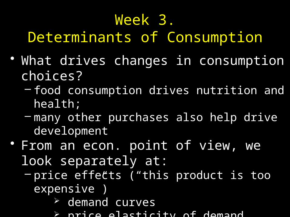
Week 3.Determinants of Consumption

• What drives changes in consumption choices? – food consumption drives nutrition and health; – many other purchases also help drive development

• From an econ. point of view, we look separately at:– price effects (“this product is too expensive”)

demand curves price elasticity of demand

– income effects (“my income is too low”) income-consumption (Engel) curves income elasticity of demand

…and then consider lots of other factors as well!

The Demand Function

Lots of factors could influence quantities consumed;

mathematically, for any one good (Q1):Q1 = f (...)

What should be in the function? For example, for the quantity of wheat…

Qwheat = f (...)How about for the quantity of pork?

Qpork = f (...)…or potatoes?

Qpotatoes = f (...)

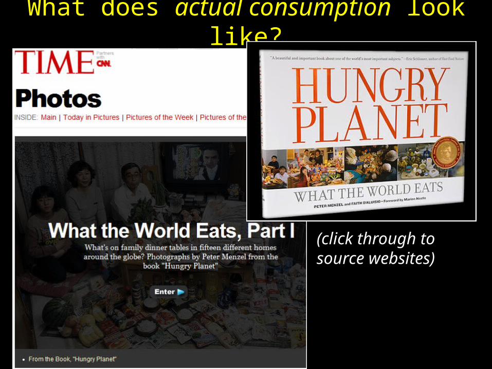
What does actual consumption look like?

(click through to source websites)

Luxembourg: The Kuttan-Kasses of Erpeldange

Food expenditure for one week: 347.64 Euros or $465.84

USA: The Revis family of North Carolina

Food expenditure for one week: $341.98

Japan: The Ukita family of Kodaira City

Food expenditure for one week: 37,699 Yen or $317.25

UK: The Bainton family of Cllingbourne Ducis

Food expenditure for one week: 155.54 British Pounds or $253.15

United States: The Fernandezes of Texas

Food expenditure for one week: $242.48

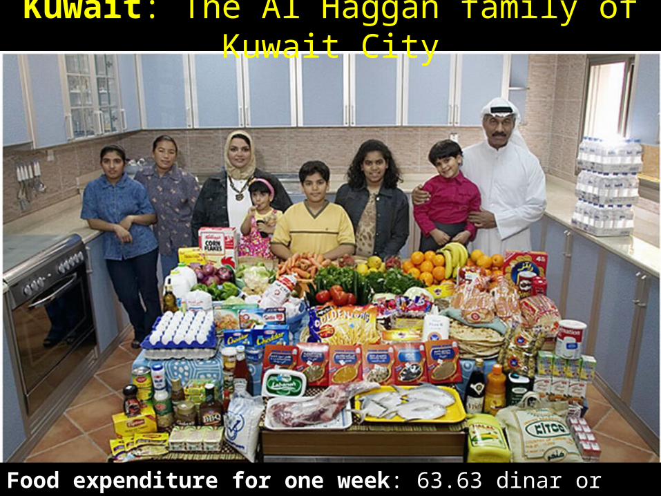
Kuwait: The Al Haggan family of Kuwait City

Food expenditure for one week: 63.63 dinar or $221.45

Mexico: The Casales family of Cuernavaca

Food expenditure for one week: 1,862.78 Mexican Pesos or $189.09

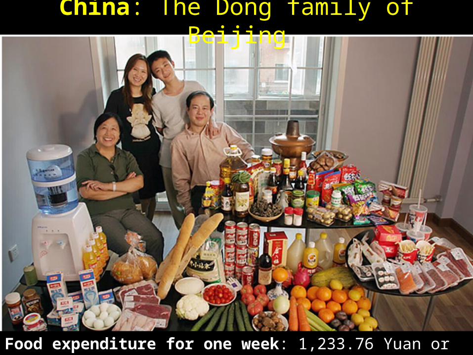
China: The Dong family of Beijing

Food expenditure for one week: 1,233.76 Yuan or $155.06

Poland: The Sobczynscy family of Konstancin

Food expenditure for one week: 582.48 Zlotys or $151.27

Guatemala: The Mendozas of Todos Santos

Food expenditure for one week: 573 Quetzales or $75.70

Egypt: The Ahmed family of Cairo

Food expenditure for one week: 387.85 Egyptian Pounds or $68.53

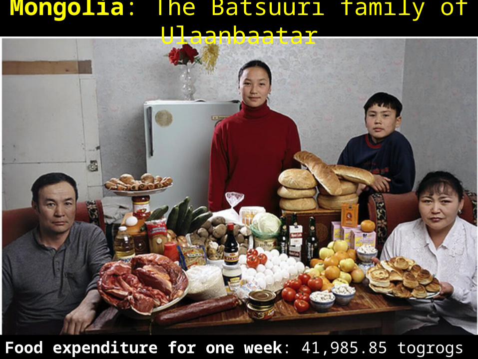
Mongolia: The Batsuuri family of Ulaanbaatar

Food expenditure for one week: 41,985.85 togrogs or $40.02

India: The Patkars of Ujjain

Food expenditure for one week: 1,636.25 rupees or $39.27

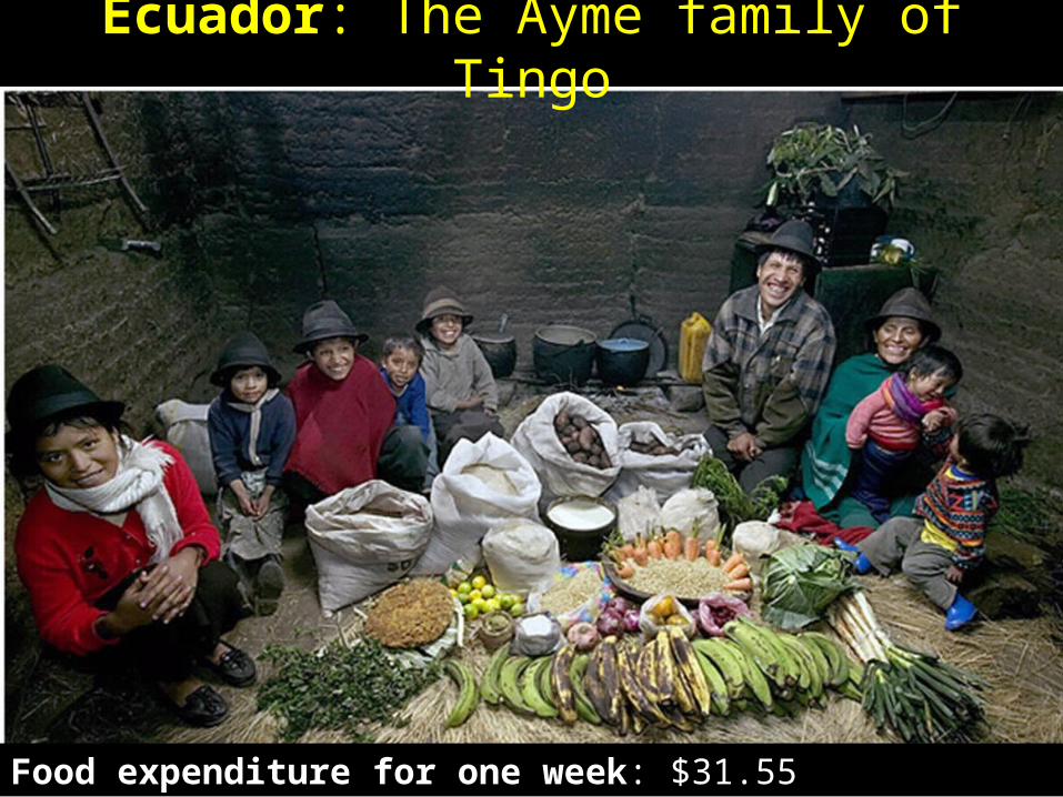
Ecuador: The Ayme family of Tingo

Food expenditure for one week: $31.55

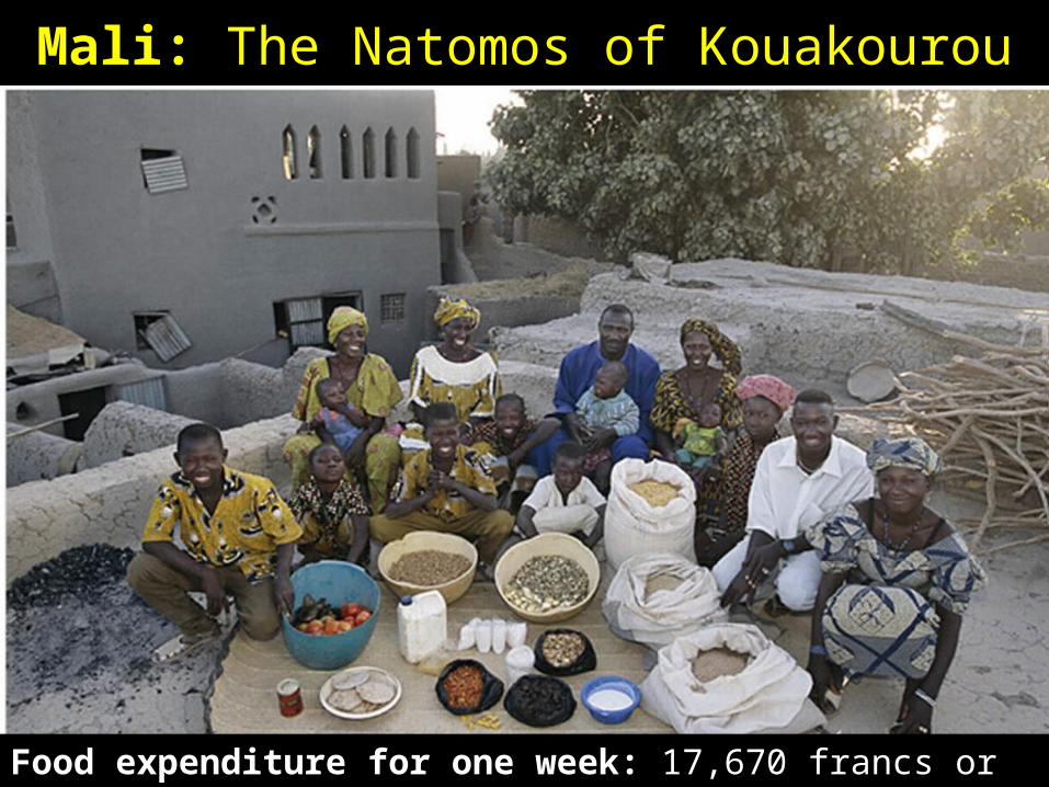
Mali: The Natomos of Kouakourou

Food expenditure for one week: 17,670 francs or $26.39

Bhutan: The Namgay family of Shingkhey

Food expenditure for one week: 224.93 ngultrum or $5.03

Chad: The Aboubakar family of Breidjing Camp

Food expenditure for one week: 685 CFA Francs or $1.23

What explains differences and changes in consumption during economic development?

Now back to economics…

Week 3.Determinants of Consumption

• What drives changes in consumption choices? – food consumption drives nutrition and health; – many other purchases also help drive development

• From an econ. point of view, we look separately at:– price effects (“this product is too expensive”)

demand curves price elasticity of demand

– income effects (“my income is too low”) income-consumption (Engel) curves income elasticity of demand

…and then consider lots of other factors as well!

The Demand Function

Lots of factors could influence quantities consumed;

mathematically, for any one good (Q1):Q1 = f (...)

What should be in the function? For example, for the quantity of wheat…

Qwheat = f (...)How about for the quantity of pork?

Qpork = f (...)…or potatoes?

Qpotatoes = f (...)

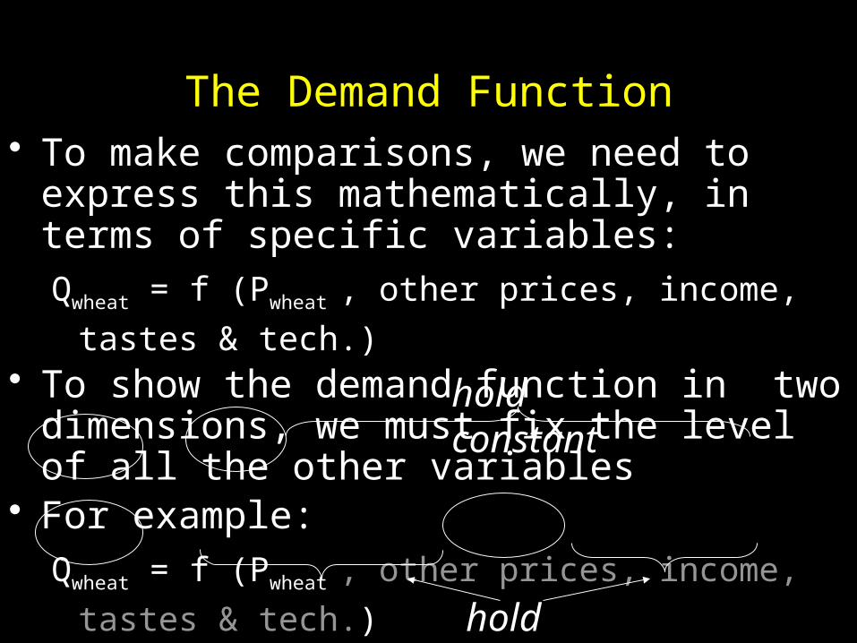
The Demand Function• To make comparisons, we need to express this

mathematically, in terms of specific variables:

Qwheat = f (Pwheat , other prices, income, tastes & tech.)

• To show the demand function in two dimensions, we must fix the level of all the other variables

• For example:

Qwheat = f (Pwheat , other prices, income, tastes & tech.)orQwheat = f (Pwheat, other prices, income, tastes & tech.)

hold constant

hold constant

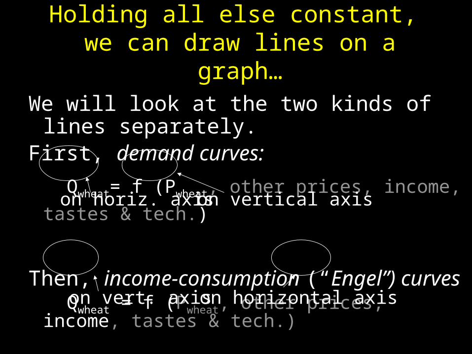
Holding all else constant, we can draw lines on a graph…

We will look at the two kinds of lines separately.First, demand curves:

Qwheat= f (Pwheat, other prices, income, tastes &

tech.)

Then, income-consumption (“Engel”) curvesQwheat = f (Pwheat, other prices, income, tastes &

tech.)

on horiz. axis on vertical axis

on vert. axis on horizontal axis

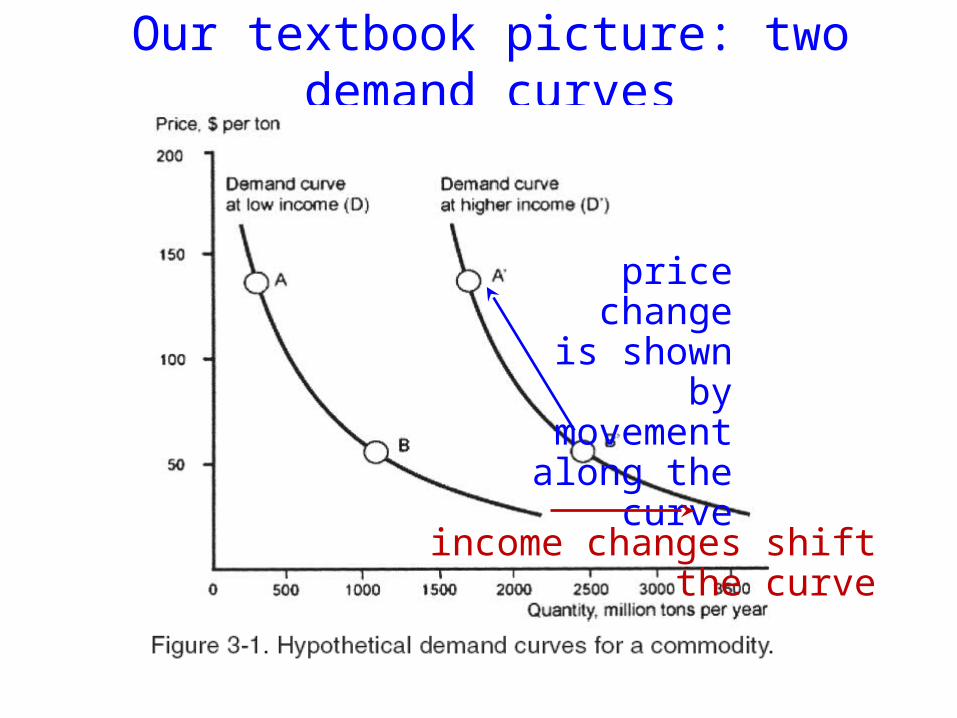
Our textbook picture: two demand curves

price changeis shown by

movement along the

curve

income changes shift the curve

slope = rise / run ≈ 100 / -500 = -0.2 units are $/ton per mt/yr

elasticity = %∆Q / %∆P = (∆Q/Q) / (∆P/P) ≈ 500/2500 / -100/50 = .2 /-2 = -0.1 = 10%

How can we measure these curves?

no units, so we can make comparisons!

Can we make comparisons that eliminate units?

We also need income elasticities of demand

but how big wasthis income change?

n = %∆Q / %∆I ≈ 1500/500 / 1000/250 = 3 / 4 = 0.75 =75%

…let’s say it was from 250 to 1000 $/yr :

again, no units so

we can make comparisons!

Demand follows fairly regular laws:

In response to price, note:--The “law of demand”: demand curves slope down

» price elasticities of demand are negative

( E < 0) » higher prices lead to lower quantity consumed

--Food demand is usually “price-inelastic”» quantity consumed changes less than price

( |E| < 1)» higher prices lead to more total expenditure

In response to income, note:--Food demand follows “Engel’s Law”: grows slower than income

» income elasticity of demand is often less than one

( n < 1) » higher income allows a lower share of it spent on food

--Staple food follows “Bennett’s Law”: grows slower than other food» income elasticities are especially low

( |nstaples| < |nothers| )

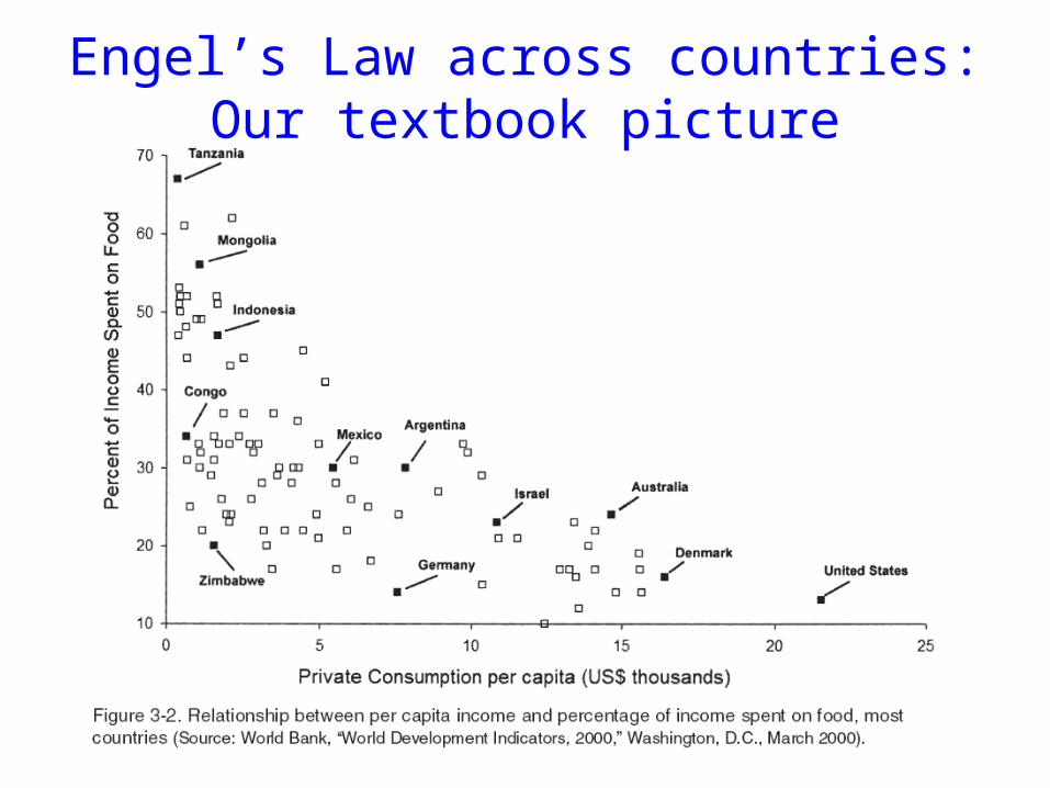
Engel’s Law across countries:Our textbook picture

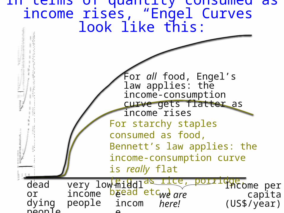
In terms of quantity consumed as income rises, “Engel Curves” look like this:

For starchy staples consumed as food, Bennett’s law applies: the income-consumption curve is really flat(e.g. as rice, porridge, bread etc.)

For all food, Engel’s law applies: the income-consumption curve gets flatter as income rises

deador dyingpeople

very low-incomepeople

middle-incomepeople

Income per capita (US$/year)we are here!

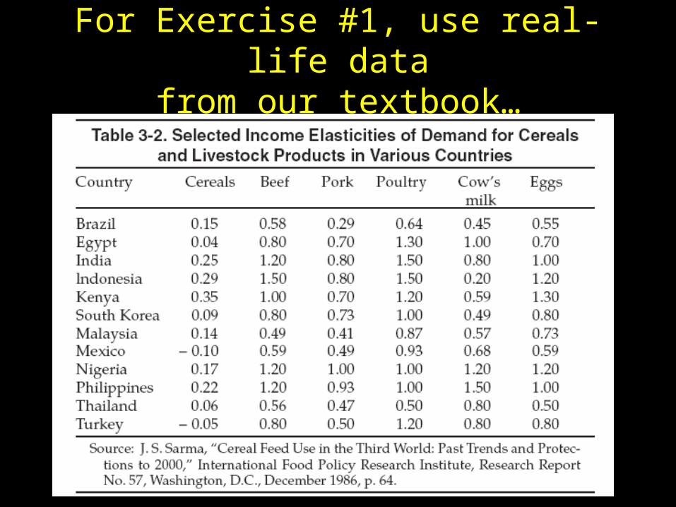
For Exercise #1, use real-life datafrom our textbook…

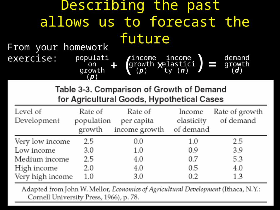
Describing the past allows us to forecast the future

From your homework exercise:population

growth (p)

income growth

(p)

income elasticity

(n)

demand growth

(d) x =+ ( )

But reality is more complicated! How has U.S. consumption actually changed

with our income growth?

0

500

1,000

1,500

2,000

2,500

3,000

1970

1972

1974

1976

1978

1980

1982

1984

1986

1988

1990

1992

1994

1996

1998

2000

2002

2004

2006

Added Sugars

Added Fats

Cereals&Flour

Fruit&Veg.

Dairy

Meat, eggs, and nuts

Source: Calculated from the Loss-Adjusted Food Availability estimates of the USDA/Economic Research Service (www.ers.usda.gov/Data/FoodConsumption). Data last updated March 15, 2008.

Estimated total food consumption in the U.S.,1970-2006(calories per capita, by source)

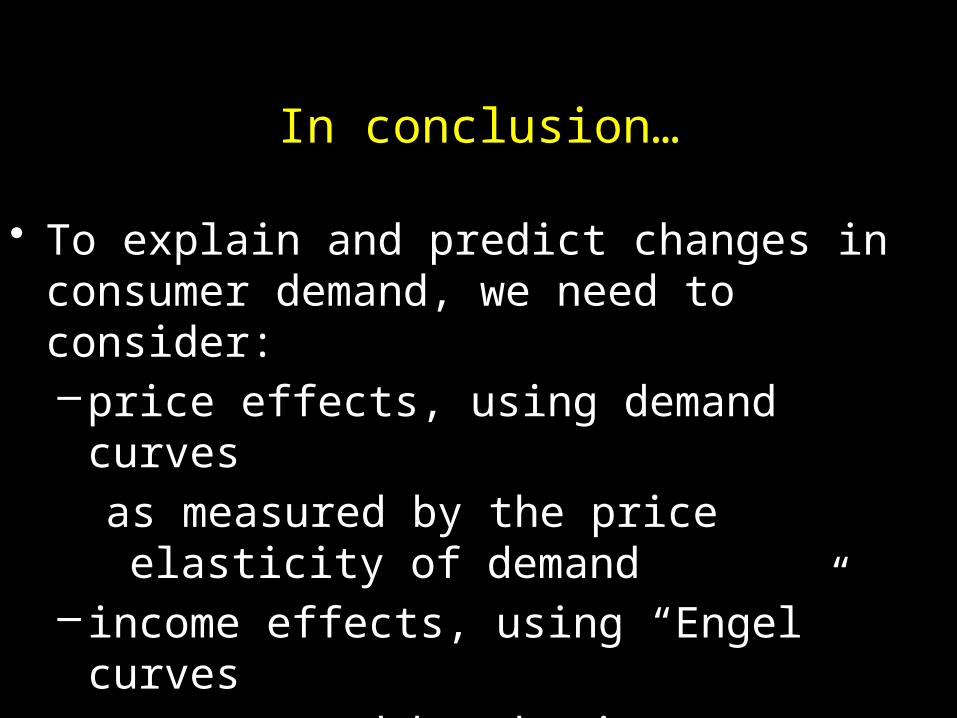
In conclusion…

• To explain and predict changes in consumer demand, we need to consider:–price effects, using demand curves

as measured by the price elasticity of demand– income effects, using “Engel” curves

as measured by the income elasticity of demand–…and then consider many other factors that can

shift these curves over time or across countries.