What Drove 19th Century Market Integration?

David S. Jacks Department of Economics One Shields Avenue UC Davis Davis, CA 95616

2

I. INTRODUCTION

For a number of years, the process of commodity market integration has proven to be an

area of abiding theoretical and empirical interest. Long-standing deviations from the Law of

One Price (LOP) have been documented for a remarkably wide range of geographic areas and

time periods.

As of late, the literature on the topic has been reoriented, primarily due to the work of

Engel and Rogers (1995, 1996) and McCallum (1995). The shared hypothesis of these two lines

of work is that there is a pernicious and persistent border effect, both in terms of commodity

price variation and commodity flows, which is registered in the data even after controlling for

such things as distance and exchange rate volatility. Although very recent work has called into

question the extent of the border effect in relation to the impediment of physical flows of goods

(Anderson and van Wincoop, 2003), the ubiquity of a border effect in the determination of

relative price volatility seems inescapable (cf. Engel and Rogers, 2001; OConnell and Wei,

2002; and Parsley and Wei, 1996, 2001a,b).

The common strand linking this literature is the attempt to explain the degree of

commodity market integration through the use of a handful of geographic and institutional

variables. A few questions have remained unasked, and therefore, unanswered, in the literature.

Are the forces at work identified in the contemporary literature indicative of commodity market

integration in other periods? More importantly, what may we take as the proximate causes of the

evolution of commodity market integration?

To answer these questions, we propose to broaden the temporal scope of the existing

literature by considering another period of nascent globalization, namely the long 19th Century.

In the past decade, the 19th century has received a new wave of interest and inquiry as

3

researchers have repositioned the period as one of so-called early globalization. Thus, the corpus

of work by ORourke, Williamson, and others has directed the attention of economic historians

and economists alike back to this time of unprecedentedand in many respects, unsurpassed

integration of global commodity, capital, and labor markets (ORourke and Williamson, 1999).

This paper takes as it aim to act as a bridge between the contemporary trade literature and the

study of economic history.

The fundamental results are, first, we are able to not only align our results with the

received wisdom but also identify further variables which have been relatively underrepresented

in the literature: proxies for technological change; enduring, trade-enhancing geographical

features associated with navigable waterways; and the choice of monetary regime.

Second, we find that splitting commodity market integration into the sub-processes of

price convergence and synchronization is justified as all of our results confirm the fact that two

different sets of causal factors predominant in each case. Most surprisingly, institutional and not

technological variables dominate the former. And while a more balanced set of factors is at play

in the latter case, the role of technological change is much more muted than previously supposed.

Finally, intertemporal analysis allows us to not only expound upon the most significant

factors under consideration but also the rich variety of experience partially masked by our panel

results. The sub-sample results are found to be consistent with our maintained thesis that

traditional explanations of the evolution of market integration have been overly reliant on

technological change as an explanatory variable, given the apparently more substantive role of

the organization of trade.

By way of conclusion, we draw implications from these results which we find to be far

from trivial. First, given that current disparities in economic development worldwide are best

4

explained in terms of a dynamic process which extends far into the past, the degree to which

institutions or technology matters in terms of getting prices right through market integration is

essential, in the sense that the promotion of markets has long been a tacit, if not explicit, goal of

many development agencies. Second, the recent work of Acemoglu et al. (2002a,b) proposes a

path of causality stretching from (geographically-dependent) trade to institutional change to

economic growth. The results proffered here suggest another line of thinking, namely that trade

itself could potentially be a function of existing institutions. Thus, Acemoglu et al.s explanation

for the rise of Europe would necessarily be incomplete as the path of causality would again

originate from institutions.

The rest of the paper is structured as follows. Section II positions the paper with respect

to the context of commodity market integration as well as outlines the various measures and

techniques employed throughout the study. Section III briefly details the construction of our

data. Section IV presents and discusses our empirical results while section V concludes.

II. ANALYTICAL FRAMEWORK

Following the contemporary literature on the empirical irregularities of the Law of One Price, we

split the concept of market integration into the related but distinct sub-processes of price

convergence and price synchronicity.

Generally, it is suggested that price convergence is the sine qua non of market integration

as the fundamental issue at hand is the formulation of an intra- and inter-national division of

labor. Of course, this process is predicated upon the successful transmission of price signals to

the constituent economies, i.e. with no tendency for prices to equalize, the process of market

integration is a meaningless concept. However, it does not necessarily follow that the

observation of price convergence alone can be taken as proof of economically significant market

5

integration, as prices may be influenced by processes outside of the realm of economic

transaction and exchange (e.g., climatological events).

What is needed is some idea of the interrelationship among price systems (or series),

specifically how they dynamically adjust to shocks in other markets. Price synchronization can

then be viewed as a supplementary element in the process of market integration. To this end, we

propose the simultaneous consideration of these two independent conditions, convergence and

synchronization, as the proper approach to studies of market integration.

ON THE SYNCHRONICITY OF PRICES

Fairly dramatic developments have occurred in furthering our understanding of precisely how to

model price synchronization in market integration. What we have specifically in mind is a class

of econometric models for goods market arbitrage that explicitly account for those elements

thought to be most important in determining the degree of market integration, namely time and

space. As has been shown (cf. Obstfeld and Taylor, 1997; Prakash, 1996; and Prakash and

Taylor, 1997), those studies of market integration based on the absolute Law of One Price (LOP)

fail to compensate for the elements of transportation and transaction costs associated with trade

and, hence, proffer significantly biased results.

In order to capture the effects of transportation and transaction costs, the model to be

used incorporates a band equilibrium whereby prices in one market vis-à-vis those in another

market are allowed a certain degree of latitude not allowed for in other models of market

integration: if prices are outside the band equilibrium they will adjust, but if prices are inside the

band price movements will be random. Further innovations to this model include asymmetric

responses in the respective markets due to route-specific transportation and transaction costs

6

(Ejrnæs and Persson, 2000) and the modeling of storage strategies on the part of arbitrageurs

(Coleman, 1995).

Sparing some of the details and referring the interested reader to Appendix I, we can state

that for any pair of localities, the change in price in one locality at time t, )( 11

11−−=∆ ttt PPP ,

should be negatively related to the level of the margin between the two localities in the previous

period t-1, )( 21

11

121 −−− −= ttt PPM , if the margin exceeds the band of transaction/transportation costs,

),( 211

121 −− tt CC .1 If the margin is less than the band of transaction/transportation costs (i.e., the

thresholds), the change in price is free to follow a random walk within the corridor between the

two bands. The asymmetric-threshold error-correction-mechanism (ATECM) is then given by:

(1) =∆ 1tP

−<++

≤≤−

>+−

−−

−

−−

12121

1121211

21121

121

21121

1211211

)(

)(

CMifCM

CMCif

CMifCM

ttt

tt

ttt

ηρη

ηρ

(2) =∆ 2tP

−<++

≤≤−

>+−

−−

−

−−

21211

2212112

12211

212

12211

2122112

)(

)(

CMifCM

CMCif

CMifCM

ttt

tt

ttt

ηρη

ηρ

where ( ) ( )Ω,0~, 21 Nidtt ηη . The sum of the ρ-coefficients (designated as rho below) will equal

zero in the case of no integration and negative one (or below) in the case of perfect integration.2

1 In what follows, we will remain agnostic as to the form and composition of the transaction costs term. Although certain elements can easily be enumerated as belonging in the set of transaction-cost determinants (i.e. transportation costs, brokerage costs, storage costs, tariffs, taxes, and spoilage), others remain decidedly recalcitrant in terms of incorporating them into the present model (i.e. exchange rate risk, prevailing interest rates, the risk aversion of agents, and the quality of information available). As such, we will interpret the transaction cost term in an appropriately broad fashion. 2 Conceptually, the summed coefficients may indeed exceed unity in that the concept of the corridor of inaction implies that we can observe price movements in excess of the initial price margin; here, a simple numerical example might be instructive. Let city A in time t-1 have a price of $10 and city B a price of $5; the transaction costs associated with transporting the good from A to B is $5 while the costs from B to A are $3; finally, the price in A and B in time t are $7.60 and $7.10, respectively. Basic algebra reveals that the sum of the coefficients on ρ must be less than 1. As we will see below, this is hardly a pedantic exercise as we actually observe estimates lower than -1.

7

With no closed form solution available due to the non-linearity introduced by the

thresholds, estimation takes place by maximization of the likelihood function via a grid search on

the observed price differentials. In this case, the likelihood function should follow that of the

SUR estimator, or namely

∑=

−Ω−Ω−−=T

ttt

TTML1

1'

21log

2)2log(

2log)3( ηηπ ,

where T = number of observations and M = number of equations (here, 2).

Naturally, this type of highly-detailed modeling does come at a cost, in terms of the need

for high frequency price data. Add to this the wide-ranging geographic and temporal scale of our

project and the data requirements become truly prodigious. To avoid compounding the

dimensionality of the project, the focus will exclusively be on the intra- and inter-national

markets for (constant-quality-adjusted) wheat. Motivating this choice of commodities is an easy

task: throughout the 19th Century, the intra- and inter-national markets for wheat can be taken as

high watermarks for commodity market integration due to the heavy weight of wheat in

production, consumption, and commerce alike. Appendix II below summarizes the coverage and

sources of the dataset.

ON THE CONVERGENCE OF PRICES

Returning to the economically substantive aspect of market integration, our attention now turns

to the means of assessing the degree of price convergence. As a starting point, it is suggested

that we make use of the output generated from the ATECM model above, as one of the chief

attractions of the model is that it provides estimates of the combined transportation and

transaction costs directly based on observed price differentials. Thus, if for any particular pair of

cities we observe that the estimated transaction cost parameters decline through time, it can be

8

inferred that the level of the price differential between the two cities has fallen as well.

Additionally, coupled with information on the general level of prices, we can scale our estimates

of the transaction costs by the average price for the corresponding city-pair and time horizon in

order to arrive at a unit-less measure of price convergence (designated as reltc below)

appropriate for the type of cross-country comparisons we would like to make.3

III. DATA CONSTRUCTION

To assess the intranational components of price synchronicity and convergence, the first

step is to construct a matrix of prices of dimension n (the number of cities; generally twelve) by t

(generally, 11 years, for 132 observations) and to form all pair-wise combinations of cities in the

set of prices in order to arrive at estimates of our asymmetric ρ-coefficients (or adjustment

parameters) and the transaction costs (divided by average price) inferred from the behavior of the

data. The next step was to then record these estimated parameters. The final step was to iterate

this procedure at 5-year steps for each country; thus, for a country like the United Kingdom for

which we have a full panel of 12 cities for 114 years, we began in the period of 1800-1810 and

ended in that of 1905-1913 with 20 intervening observations on the course of market integration

(thus, T=22).

As to the international component, we in large part followed the precedent set above on

intranational market integration. Here, instead of constructing our variables from observations

3A further measure of price convergence used extensively in the contemporary literature (cf. Engel and Rogers 1995, 1996; and Parsley and Wei, 2001a, 2001b) is defined as the variance of the logged relative price over a given time horizon, or

).ln(,,kT

jTTkj P

PVarV =

This measure was constructed for the database at hand and explored under all regression specifications discussed below. Given the high degree of correlation between this variance term and the reltc variable (R>.90), it will come

9

formed from every pair-wise combination available in any given country, it was decided that the

panels of price data for each country should be matched with prices from a set of 5 cities

(Bruges, London, Lwow, Marseille, and New York City), all of which represent important

markets for wheat in the international economy and for which data exists over the entire period.4

Apart from this distinction, our methodology was identical to that identified previously: estimate

our asymmetric ρ-coefficients and the transportation/transaction costs (divided by average price)

inferred from the behavior of the data; record the average value of these estimated parameters;

and iterate this procedure at 5-year steps for each country.

Finally, appropriate explanatory variables were considered and constructed. Table 1

below provides summary statistics of our dependent and independent variables. Notes on the

particulars underlying their construction made be found in Appendix III.

IV. EMPIRICAL RESULTS

To weigh the determinants of 19th Century commodity market integration, we proceed by first

considering a benchmark case inspired by the work of Engel and Rogers (1995, 1996) and

Parsley and Wei (1996, 2001a). As a unique contribution to the literature we explore not only

the two facets of commodity market integration (price convergence and synchronicity) but also

the differential effects implied by the inclusion of variables meant to capture of proxies for

technological, geographical, and institutional variations across time and space.

as no surprise that the results added little further information on the process of price convergence and, therefore, are not reported here. 4 Please note that we have fully separated out the intra-national component from our various datasets. Thus, for Spain, we compare the observations on all 12 cities available against those in our 5 sample cities whereas for France, we compare the observations on all 12 cities available against all sample cities expect Marseille.

10

BENCHMARK ANALYSIS

As mentioned before, certain researchers looking into the forces affecting market integration for

the late 20th Century have used a gravity-model-inspired framework of inquiry. Generally, this

has been implemented as a regression of the following type, taken from Engel and Rogers

seminal work (1996):

(4) kj

n

mmmkjkjkj uDBrPV ,

1,2,1, )( ∑

=

+++= γββ ,

where the dependent variable equals the variance of the logged price ratio in cities j and k, rj,k is

the distance between cities, Bj,k indicates a border between the two cities (i.e., a dummy for

international exchange), and Dm is a dummy variable for each city in the sample. Additions to

this model have included trade barriers and regional dummies (Engle and Rogers, 1995), of

lagged dependent variables (Parsley and Wei, 1996), of the difference of the changes in the

logged prices as the dependent variable (Parsley and Wei, 2001b), and of a squared distance term

(Engel and Rogers, 2001).

Here, we follow in broad form the same exercise, but with a view towards more explicitly

modeling the structure of errors. Typically, estimation of equation (5) has taken place within the

framework of OLS estimation with partial attempts to control for heteroscedasticity (via fixed-

effects estimation or the use of city dummies) and the possibility of serial correlation when using

time series (via the inclusion of the lagged dependent variable). What we propose is the use of

GLS estimation,5 explicitly incorporating group-wise heteroscedasticity (based on country-

5 GLS estimation also has the desirable property of controlling for the fact that our dependent variables are themselves estimated variables. Given a properly defined set of weights on observations, the GLS estimator is consistent and unbiased (see Saxonhouse, 1976).

11

rather than city-pairs) and serial correlation6 into the structure of the variance-covariance matrix.

Thus, our baseline results come from the following regression:

(6) Tkjt

TTkjTkjkjkjTkj uDborderevoldistsqdistnIntegratio ,,

22

1,4,,3,2,1,, ∑

=

+++++= γββββ ,

where the dependent variable is time-specific and is defined either as one of our measures of

market integration (i.e., the transaction-cost-adjusted adherence to the LOP (ρ) or the estimated

relative transaction cost); the first two terms on the right-hand side, distj,k and distsqj,k, refer to

distance and squared distance variables, respectively; evolj,k,t is the variance of the logged

nominal exchange rate between the currencies of j and k in time t; borderj,k denotes the existence

of a border between j and k; and Dt is a set of time dummies.

Furthermore, a suitable weighting matrix for the dependent variables must be specified in

order to implement our estimator with group-wise and serially-correlated disturbance terms. In

all results reported below, the weights used were the differences between one and the p-value of

each city-pair regression (calculated according to the methodology set out in Appendix III) for

the relative transaction cost and LOP-adherence terms.7

The results from this initial regression are reported in Table 2 below. The patterns look

sensible. Price convergence (as measured inversely by relative transaction costs) decreases with

distance, nominal exchange rate volatility, and the border. The degree of price synchronization

(as measured by ρ) decreases as these same variables rise.

6 As a further corrective for the possibility of serial correlation, we also estimated our models on non-overlapping observations. In this case, the results were not fundamentally altered, although this approach entailed a general loss of power, especially when we consider our model on sub-samples (see below). Consequently, we opt for using all available data and correcting for serial correlation as described above. 7 It should also be noted that the results presented are seemingly invariant to any set of plausible weights selected, such as the value of summed squared errors, log-likelihoods, and F-test values.

12

TECHNOLOGY

One of the most noticeable gaps in the existing literature is any consideration of technological

change. Understandably, this gap is primarily a function of the limited time horizons considered

(i.e., the 1990s) in which one would reasonably expect no fundamental changes in the

technology of transport or transaction. Here, we make a unique contribution to the literature by

attempting to successfully integrate technological change into our analysis.

As even the most cursory review will reveal, the historical literature for the 19th Century

seems to be dominated by certain key themes, namely the development of intra- and inter-

national communication and transport networks. In this account, the dynamic twins of the

railroad and telegraph take pride of place in creating economically and socially unified polities.

In order to assess the validity of the various untested claims made about the efficacy of

railroads, in particular, in forming coherent national and international markets, we have

constructed a series of variables which capture the historical development of American and

European rail networks. These variables take the form of indicator variables which switch on

with the completion of an inter-city rail connection.

The effects of including one of these variables, rr1, along with an interaction term with

distance, rrdist, on our initial results are reported in the first panel of Table 3 below.8 The rr1

variable proves to be significant in the case of both price convergence and synchronization. The

motivation for including our interaction term, rrdist, is that a railroad between Maddaloni and

Naples (our shortest rail route at 30 km.) may have had a different impact than that between

Samara and Brugges (our longest route at 8080 km.) The results in Table 3 bear out this

8 This variable, rr1, indicates the existence of a railroad connection in any year of the eleven years considered. The railroad indicator was variously defined to indicate the existence of connection in a majority of years (rr2) and all years (rr3) in order to potentially capture a delay in the general diffusion of railroad use. All specifications reported were ran with these alternate variables with no material effect on the estimated coefficients.

13

suspicion. The interaction of railroads with distances is significant, simultaneously promoting

price convergence and muting price synchronization as distance increases.

A further issue to be addressed is one touched off forty years ago by Fogel (1964).

Briefly, the debate revolves around the question of what was the incremental contribution of

railroads over and beyond that of canals. Given the extensive and expandable canal network in

the United States prior to the establishment of railroads, it was Fogels argument that this

incremental contribution of railroads was small. The results presented here are surprising in that

they confirm Fogels skepticism, albeit in a way not addressed in the original debate. Whereas

the original argument was framed in terms of the contribution of railroads to economic growth

via investment demand and social savings via lower transportation costs, what the second panel

of Table 3 implies is that while canals contribution to price synchronization was overshadowed

by that of railroads, canals were associated with lower thresholds.9

Finally, to assess technological change in maritime shipping, exploratory regressions

were ran on the variables included in our final specification (see below) along with an interaction

term between time and a dummy on port city-pairs (ports). The results of these exercises are

depicted in Figures 1 & 2 which plot the sum of the coefficients attached to this interaction term

along with those associated with the original set of time dummies. Broadly, they offer a very

compelling story of the integration of ports through time: following the turbulence of the

Napoleonic Wars, prices were strongly converging until mid-century at which time integration

slowed while price synchronization saw no deterministic pattern. These results imply that

technological change in the maritime industry (read steamships) may have had far more muted

9 In a preliminary exercise, an interaction term between canal and distance was employed. The estimated coefficients were highly insignificant. This was a pattern repeated with other potentially distance-related variables, i.e. rivers and ports. Throughout, it is only the railroad-distance interaction which performs well. Consequently, interaction terms for the other variables have been suppressed.

14

effects than previously supposed. Until we can more explicitly capture the diffusion of maritime

technology, however, these results will remain only suggestive.

GEOGRAPHY

Much of the recent literature on long-term growth patterns has tried to assess the implications of

geography for economic activity and evolutionsome finding a critical role (Sachs, 2000, 2001)

and others a negligible one (Acemoglu et al., 2002a). Without pushing the parallel too far, it can

be fairly said that one of the issues central to this debate is the degree to which geography shapes

patterns and terms of trade. Surprisingly, little work in the literature on market integration has

explicitly tried to incorporate the potential contribution of geographic features, beyond the

inclusion of distance, border, or non-adjacency variables.

We can offer a slight remedy by including indicator variables on the existence of port

facilities on both sides of our city-pairs (port) and of a shared navigable river system (river). As

can be seen in Table 4, the inclusion of these variables significantly adds to the explanatory

power of our regressions on price convergence (with the expected negative signs confirmed) and

synchronization (with the expected positive signs confirmed).

INSTITUTIONS

In this section, we will interpret the term institutions in an appropriately broad fashion to include

such variables as the choice of monetary standard, the existence of a common language, and the

outbreak of intra- and inter-state conflict. The motivation for the first two variables is that they

have been consistently shown to be strong determinants (or at least, correlated with other

unobserved determinants) on market integration and the directions and dimensions of the volume

15

of trade.10 As to the last variable, we are confronted with a literature which has focussed almost

exclusively on geographic and temporal units which are free from such incidences of war and

insurrection, so we might do well in giving them their proper do for the 19th Centurya

relatively peaceful century, but one to which the depredations of war were not unknown.

As a first pass, we consider the effects of two key variables, the emergence of the gold

standard11 and the existence of a common language, on the process of market integration. The

first panel of Table 5 clearly indicates that these two variables consistently and significantly

contribute to the total process of market integration. This is especially true for the gold standard

variable as the nearly equal but opposite coefficients respectively associated with border and gs1

in the regressions on price convergence and synchronization allow for a very tantalizing

interpretation: namely, the adoption of the gold standard resulted in the effective extension of a

countrys borders to include other nations in the gold standard club. Furthermore, as we are

already explicitly controlling for exchange rate volatility, the adoption of the gold standard must

be symptomatic of deeper integrative forces at work (Bordo and Flandreau, 2003).12

10 For an indication of the work on historical monetary standards see López-Córdova and Meissner (2003); on contemporary currency unions, see Frankel and Rose (2002), Glick and Rose (2002), and Rose and van Wincoop (2001). 11 Following the precedent set by our analysis of railroad development, the gold standard indicator was variously defined to indicate the existence of a common adherence in any year (gs1), a majority of years (gs2) and all years (gs3) in order to potentially capture delays in transmission of the effects of the gold standard. All specifications reported were ran with these alternate variables with, again, no material effect on the estimated coefficients. 12 The inclusion of these institutional variables also affected changes in some of our original estimates which are worth mentioning. First, we find that the mere existence of a railroad is now significant for price convergence while the distance-interacted railroad term has no effect. In any case, our original conclusion of the predominance of canals is borne out as the coefficient attached to the former is over twice as large as that for railroads. Second, we are confronted with the seemingly surprising result that port, although correctly signed, yields insignificant resultsand as we shall see, does so consistently in the remainder of the analysis. However, given that the distances separating river cities are generally much smaller than those separating port cities and that the river and port variables are almost exclusively delineated along the lines of intra- and inter-national trade, there seems little trouble in aligning these results with our a priori expectations. Finally, the addition of the gold standard indicator, now nullifies the effect of nominal exchange rate volatility on price synchronization, suggesting our original result was proxying for the gold standard (and its correspondingly low levels of exchange rate volatility).

16

Unfortunately, less dramatic results are forthcoming when we included the mu variable,

our indicator of the existence of a shared monetary union. In unreported exercises, mu fails to be

uniformly significant; what is more, it is also signed contrary to our priorspositively correlated

with both relative transaction costs and transaction-cost-corrected adherence to the LOP. Given

the peculiar history of monetary unions in the 19th Century, however, these results may not be

surprising. In our sample countries, we were effectively able to code up one monetary union

from 1800-1913the Latin Monetary Union which saw Belgium, France, and Italy united under

a single monetary standard based on the silver 5-franc piece. Its year of inauguration, 1865, was

an inauspicious one as the dollar price of silver was set to fall by over 55% in the next fifty years

or so. Thus, the effectiveness of the LMU in terms of its purported stabilizing properties was

severely circumscribed. In what follows, we, therefore, will omit the mu variable from our

regressions.

The final element we will consider under the heading of institutions is the outbreak of

intra- and inter-state conflict. Again, the contemporary literature is noticeably silent on the issue,

given its relatively limited geographic and temporal scope. Using data collected under the

auspices of the Correlates of War project, we were able to code up suitable indicator variables

for the occurrence of war, capturing the effects of intra- or inter-national conflict on the internal

economy (intrawar), of one countrys neutrality in the face of a time of war for a trading partner

(neutral), of the outbreak of open conflict between trading partners (atwar), and finally, of the

outbreak of open conflict between trading partners and a common enemy (allies).

The results of this exercise are reported in Table 6. Of the two specifications, it is the

price convergence regression which performs best with respect to all variables. Thus, we find

intrawar and neutral to be insignificant but correctly signed while the atwar and allies variables

17

are significant and consistent with reasonable priors. As to price synchronization and its

response to intra- and inter-state conflict we are first confronted with a lack of priorsthe

justifications conceivably associated with price convergence (or divergence) are not as apparent

in this case. The intrawar and neutral variables yield results congruent to those of price

convergence. The results that atwar was associated with higher levels of price synchronization

than allies is somewhat puzzling, but citing our lack of priors these results must be accepted until

a more finely-grained analysis is explored (see below).

Rounding things out, Table 7 below summarizes our preferred specification into a more

easily translated format. Decomposing the effects of standard-deviation or discrete changes in

the independent variables on the various measures of market integration, we can come to a few

conclusions regarding the relative contributions of technology, geography, and institutions.

First, the sub-process of price convergence was dominated by institutional factors (gs1 and

comlang) with a healthy contribution of geographic factors (if we consider border to be a

geographic variable) and little contribution from technology. Second, the sub-process of price

synchronization represents a much more balanced account as institutions cede some of their

pride of place, most notably to technology. Finally, we can see that across all independent

variables the gold standard alone acted as a means to deconstruct the artificial geographic

barriers implied with national borders.

INTERTEMPORAL COMPARISONS

Having explored the pooled results of our panel data, we might do well to step back and ask

whether the results we found for the aggregate hold in discrete sub-periods. To this end, we ran

our preferred specification on three easily demarcated eras (i.e., the pre-railroad and pre-gold-

18

standard, the pre-gold-standard but post-railroad, and the post-railroad and post-gold-standard

eras).

In table 8 below, these disaggregated results are presented for the transactions-cost-

adjusted adjustment parameters (rho) and the relative transactions costs (reltc) in Panels A and

B, respectively. The changes in specification and sample suggest not only that inference from

our panel estimates is generally valid, but also allow for some further insights into the process of

integration.

With respect to rho, we will limit ourselves to two observations. First, what is most

striking about the results of this exercise is the marked failure of our independent variables to

explain the variation in rho in the period from 1800 to 1830. We can partially justify this poor

performance in light of the enormous disruption caused by the Napoleonic Wars, thus, providing

the first explicit demonstration of the price effects of the wars (Findlay and ORourke, 2003).13

Second, the two variables, border and port, appear to have become more prominent through

time. This result is somewhat surprising in that our priors would lead us to believe that the

simultaneous action of increasing economic interaction along with the development of internal

transport linkages would have sapped, not augmented, the variables force.

Turning to reltc, the disaggregated results tell some interesting stories. To begin, we can

see that intra- and inter-state conflict served to aggravate the convergence of prices more at the

end than the beginning of the period. This probably reflects the high degree of mobilization

attendant with the Napoleonic Wars, but again, this is a topic open for discussion. Second, the

insignificance of the port variablein spite of its earlier contribution to convergenceraises

further suspicions regarding the true effect of maritime technology in fundamentally altering the

13 Furthermore, the notable insignificance of evol and port in the panel estimates seem to be explained by this generalized failure as well.

19

course of market integration, citing the fact that widespread adoption of steam technology came

only after 1870. Our results suggest this adoption had little discernible impact on narrowing

price differentials in the Atlantic economy. In a similar vein, the question of the efficacy of

technological change in the form of railroads is demonstrated in the reversal of signs and

significance attached to rr1 and rrdist from 1830-1872 to 1872-1913. The story emerging is one

which challenges the received wisdom in which railroads played a singular role in conquering

time and space and, thus, creating factor and output markets of unprecedented scale.

V. CONCLUSION

Building on the insights provided by the contemporary literature on the determinants of the

extent of commodity market integration, we have attempted in this paper to lay a framework for

assessing the determinants of the evolution of commodity market integration.

First, we have been successful in determining a number of variables which undoubtedly

figured heavily in determining the pace of market integration. Among these were variables

recognizable from the contemporary literature such as controls for distance, exchange rate

volatility, common languages, and the border effect, thus, verifying the commonality of

experience with commodity market integration in the 19th and 20th Centuries. Additionally, we

have been able to identify further variables which heretofore have been relatively

underrepresented in the literature: the establishment of inter-city railroad linkages (our proxy for

technological development); enduring, trade-enhancing geographical features associated with

navigable waterways; and the classical gold standard. Furthermore, we have been able to lay

some foundations for more precisely determining the effects of intra- and inter-state conflict as in

the course of market integration.

20

Second, we have been able to justify our decision of splitting commodity market

integration into the sub-processes of price convergence and price synchronization as all of our

results have confirmed the fact that two different sets of causal factors predominant in each case.

The fundamental sub-process of price convergence seems to be more responsive to changes in

institutional and (to a lesser extent) geographic variables than changes in the underlying

technology of trade. Running somewhat counter to this finding, we note that the sub-process of

price synchronization represents a more balanced account as technological, geographic, and

institutional variables all seem to play a part. In any case, we see that explanations of market

integration in terms of exogenous, technological change (and railroads, in particular) has unduly

diverted our attention from analyzing the more important endogenous elements of the

organization of trade and its institutional apparatus.

Finally, intertemporal analysis allows for an even greater sense of not only the most

significant factors under consideration but also the rich variety of experience partially masked by

our panel results. Chief among the findings in this respect were the continued relevance of many

of the variables identified in the panel exercises as well as more results consistent with our

maintained thesis that traditional explanations of the evolution of market integration have been

overly reliant on technological change as an explanatory variable, given the apparently more

substantive role of the organization of trade.

The implications from these results are interesting in at least two respects. On the one

hand, if current disparities in economic development worldwide are best explained in terms of a

dynamic process which extends far into the past, the degree to which institutions or technology

matters in terms of getting prices right through market integration is essential in the sense that

21

the promotion of well-developed markets has long been, at least a tacit, if not explicit, goal of

many development agencies.

On the other hand, the recent work of Acemoglu et al. (2002a, b) proposes a path of

causality stretching from (geographically-dependent) trade to institutional change to economic

growth. The results proffered here suggest another line of thinking, namely that trade itself

could potentially be a function of existing institutions. Thus, Acemoglu et al.s explanation for

the rise of Europe would necessarily be incomplete as the path of causality would again originate

from institutions. Needless to say, this an area which demands further research.

22

APPENDIX I: THE ATECM MODEL & DIAGNOSTICS

We begin by positing the following two conditions, which encapsulate the relation of prices in two locations consistent with efficient goods-market arbitrage:

(1) 2121 CPP tt +≤ , or namely, that the price in the first location ( 1tP ) must be less than or

equal to the price in the second location ( 2tP ) plus the transaction cost associated

with physically transferring the identical good from the second to the first location ( 21C ).

What condition (1) then implies is the following inequalities: (1a.) 1221

tt PPC −≤− (1b) 2121 CPP tt ≤−

Likewise, if we reverse the order, we arrive at (2) 1212 CPP tt +≤ which, in turn, implies the following inequalities:

(2a) 2112tt PPC −≤−

(2b) 1212 CPP tt ≤− For the sake of simplicity, we can define the price margins between the two locations

as 1221ttt MPP =− and 2112

ttt MPP =− , noting that 1221tt MM −= . What the conditions, (1a)-(2b),

then imply are the following restrictions: (3) 211212 CMC t ≤≤− (4) 122121 CMC t ≤≤− To operationalize conditions (3)-(4), we state that the change in price in one market

should be negatively related to the level of the margin between the two markets in the previous period if the margin exceeds either band of transaction/transportation costs while in the corridor between the two bands the change in price is free to follow a random walk. The asymmetric-threshold error-correction-mechanism (ATECM) is then given by:

(5) =∆ 1tP

−<++

≤≤−

>+−

−−

−

−−

12121

1121211

21121

121

21121

1211211

)(

)(

CMifCM

CMCif

CMifCM

ttt

tt

ttt

ηρη

ηρ

(6) =∆ 2tP

−<++

≤≤−

>+−

−−

−

−−

21211

2212112

12211

212

12211

2122112

)(

)(

CMifCM

CMCif

CMifCM

ttt

tt

ttt

ηρη

ηρ

where ( ) ( )Ω,0~, 21 Nidtt ηη . The sum of the ρ-coefficients will equal zero in the case of no integration and negative one (or below) in the case of perfect integration.

Moving on, as 21211 CM t −<− is equivalent to 2112

1 CM t >− and 12211 CM t >− is equivalent to

12121 CM t −<− , we conveniently have three regions defined to describe the movement of the

dependent variables: I.) If 2112

1 CM t >− , then =∆ 1tP 12112

11 )( tt CM ηρ +−− and =∆ 2tP 22121

12 )( tt CM ηρ ++− .

23

II.) If 21121

12 CMC t ≤≤− − , then =∆ 1tP 1

tη and =∆ 2tP 2

tη . III.) If 1212

1 CM t −<− , then =∆ 1tP 11212

11 )( tt CM ηρ ++− and =∆ 2tP 21221

12 )( tt CM ηρ +−− . With no closed form solution available due to the non-linearity introduced by the thresholds, estimation takes place by means of maximization of the likelihood function given above via a grid search on the range of observed price differentials. DIAGNOSTIC STATISTICS

Hansen (1997) suggests a distribution theory for least-squares estimates of the threshold in a similar family of threshold autoregressive (TAR) models as well as a means of forming likelihood ratio statistics in order to gauge the relative performance of TAR models versus standard (linear) autoregressive models. The methodology developed by Hansen was adapted for use with our ATECM model. Specifically, the F-statistic was formed as:

−=

)()(

2

22*

γσγσσ

n

nnn nF ,

where the denominator equals the residual variance of the threshold model and the first term in the numerator equals the residual variance of a linear model; however, as γ (the threshold) is not identified, this F-statistic does not take a χ2 distribution. Thus, we approximate by using:

−= ∈ )(~

)(~~sup 2*

2*2**

γσγσσ

γn

nnFn nF ,

where the denominator equals the residual variance of a regression of n standard normals on the price margin (M12) and the first term in the numerator equals the residual variance of a regression of n standard normals on the price margin less the estimated transaction cost (M12-C21) . The approximation converges weakly in probability to the null distribution of the F-statistic, so we bootstrap (with 1000 replications) to approximate the asymptotic distribution and calculate:

1000

*nn FFifcount

valuep>

=− .

For the sampling distribution of the threshold estimate, we form:

−=

)()()(

)( 2

22

γσγσγσγ

n

nnn nLR ,

for every set of γ used in the grid search. Using the critical values provided by Hansen for ),(βξC we determine minimum and maximum values of Γ for which:

)()(: βγγ ξCLRn ≤=Γ . This range of values for Γ provides confidence intervals from which the standard error was calculated as:

3125.4)min(max Γ−Γabs .

An informal review of the standard errors and p-values strongly suggests the applicability and significance of the ATECM specification; for those interested, the complete set of diagnostic statistics is available from the author by request.

24

TABLE A.1: THE ATECM MODEL, DAILY VS. MONTHLY DATA, NYC-PARIS-BERLIN, 1896-1905(t-statistics reported in brackets)

PANEL A: ESTIMATION VIA PRICE LEVELSDAILY Rho Rho Threshold Threshold

City 1 City 2 for city1 for city 2 from 2 to 1 from 1 to 2 p-value Obs.Paris New York -0.0172 -0.0232 6.98 -3.02 0.0490 2940

[-230.74] [-240.66] [6.54] [-2.96]Paris Berlin -0.0224 -0.0028 2.83 0.11 0.0390 2866

[-195.62] [-63.90] [3.81] [0.13]Berlin New York -0.0120 -0.0069 4.68 -2.55 0.0411 3012

[-690.69] [-117.70] [7.47] [-4.58]MONTHLY

Paris New York -0.0303 -0.5223 6.66 -3.23 0.0739 119[-2.13] [-8.45] [2.43] [-2.79]

Paris Berlin -0.0876 -0.1666 2.47 -0.02 0.0987 119[-2.38] [-7.52] [3.56] [-0.15]

Berlin New York -0.0340 -0.2161 4.73 -2.73 0.0972 119[-2.60] [-4.09] [2.04] [-3.92]

PANEL B: ESTIMATION VIA LOGGED PRICESDAILY Rho Rho Threshold Threshold

City 1 City 2 for city1 for city 2 from 2 to 1 from 1 to 2 p-value Obs.Paris New York -0.0132 -0.0138 0.19 -0.09 0.0478 2940

[-282.23] [-169.23] [6.38] [-4.01]Paris Berlin -0.0237 -0.0053 0.06 0.00 0.0413 2866

[-270.27] [-145.31] [4.17] [.06]Berlin New York -0.0074 -0.0070 0.14 -0.08 0.0433 3012

[-720.73] [-161.94] [6.86] [-4.12]MONTHLY

Paris New York -0.0286 -0.3880 0.44 -0.23 0.1330 119[-1.55] [-7.21] [6.36] [-4.54]

Paris Berlin -0.1643 -0.1266 0.14 0.00 0.1272 119[-3.96] [-5.06] [3.67] [-0.09]

Berlin New York -0.0086 -0.2271 0.33 -0.18 0.1044 119[-1.04] [-5.43] [6.01] [-3.64]

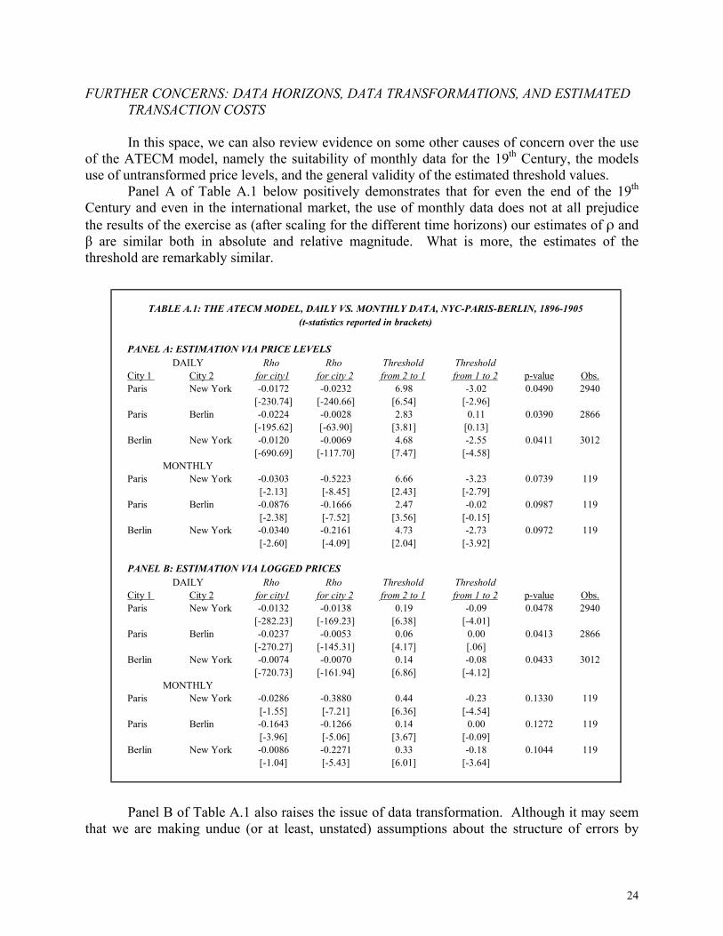
FURTHER CONCERNS: DATA HORIZONS, DATA TRANSFORMATIONS, AND ESTIMATED TRANSACTION COSTS

In this space, we can also review evidence on some other causes of concern over the use

of the ATECM model, namely the suitability of monthly data for the 19th Century, the models use of untransformed price levels, and the general validity of the estimated threshold values. Panel A of Table A.1 below positively demonstrates that for even the end of the 19th Century and even in the international market, the use of monthly data does not at all prejudice the results of the exercise as (after scaling for the different time horizons) our estimates of ρ and β are similar both in absolute and relative magnitude. What is more, the estimates of the threshold are remarkably similar.

Panel B of Table A.1 also raises the issue of data transformation. Although it may seem that we are making undue (or at least, unstated) assumptions about the structure of errors by

25

TABLE A.2:PREFERRED SPECIFICATION USING PRICE LEVELS v. LOGGED PRICESDependent Variable:

Reltc (levels) Reltc (logs) Rho (levels) Rho (logs)Independent Variables: Coefficient P>|z| Coefficient P>|z| Coefficient P>|z| Coefficient P>|z|

dist 0.027000 0.000 0.028800 0.000 -0.009150 0.000 -0.014800 0.005distsq -0.000128 0.000 -0.000674 0.045 0.000240 0.027 0.000166 0.047evol 0.741747 0.000 0.292632 0.000 0.109694 0.546 0.168250 0.662

border 0.252436 0.000 0.204645 0.000 -0.101505 0.000 -0.169718 0.000rr1 -0.017810 0.022 0.017925 0.000 0.182243 0.000 0.265532 0.000

rrdist -0.002020 0.385 -0.001340 0.663 -0.033400 0.000 -0.047800 0.000canal -0.042563 0.000 -0.029527 0.003 0.070038 0.000 0.042257 0.000river -0.035596 0.000 -0.014477 0.005 0.066407 0.000 0.042251 0.000port -0.019397 0.000 -0.018054 0.000 0.013890 0.110 0.033630 0.184gs1 -0.202311 0.000 -0.211561 0.000 0.132036 0.000 0.192747 0.000

comlang -0.137952 0.000 -0.171649 0.000 0.029355 0.020 0.037886 0.000intrawar 0.002252 0.855 0.002043 0.325 -0.093747 0.000 -0.122700 0.009neutral 0.024066 0.105 0.000835 0.609 -0.007894 0.533 -0.002465 0.354atwar 0.084237 0.002 0.130300 0.000 -0.025698 0.265 -0.047950 0.311allies -0.058264 0.018 -0.025922 0.082 -0.054341 0.004 -0.044109 0.001

N: 11576 11576 11576 11576Weighted by: (1-"p-value") (1-"p-value") (1-"p-value") (1-"p-value")

Wald χ-squared: 8750.43 3214.07 27926.99 7154.24Prob > χ-squared: 0.0000 0.0000 0.0000 0.0000

NB: Year dummies suppressed; distance coefficients scaled to 1000 km.

using the price level, we can see that, if anything, the use of logged prices is not as desirable as our original specification. This is seen primarily in the closer adherence of the estimated thresholds in daily versus monthly data in the original specification. The two specifications do, however, offer similar stories which is further demonstrated in Table A.2 below which contrasts the results of our preferred regression analysis reported above and results using a database solely composed of logged prices.

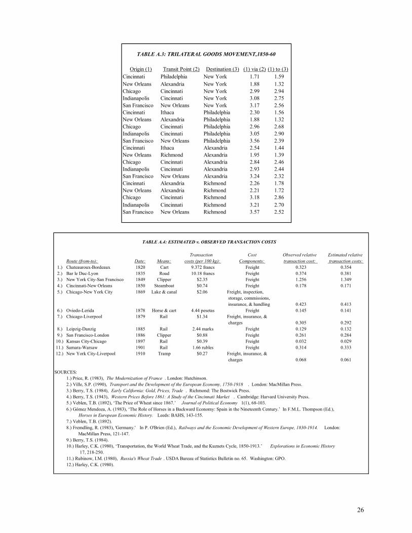
As to the validity of the estimated thresholds themselves, we consider two elements. First, we need to see that our estimates of bilateral transaction costs are consistent. Table A.3 below demonstrates that for the sample considered we see no violations of arbitrage potentials across multiple cities, i.e., 132312

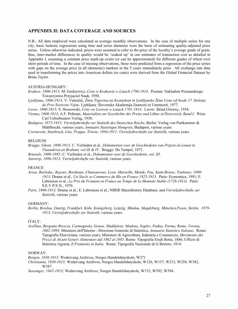
ttt CCC ≥+ . Second, we would hope to find correspondence to actual transaction costs. Table A.4 below presents compelling (albeit very limited) evidence to the effect that our estimates are indeed a good approximation to reality, especially given the wide temporal, geographical, and technological range considered.

26

TABLE A.4: ESTIMATED v. OBSERVED TRANSACTION COSTS

Transaction Cost Observed relative Estimated relativeRoute (from-to): Date: Means: costs (per 100 kg): Components: transaction cost: transaction costs:

1.) Chateauroux-Bordeaux 1820 Cart 9.372 francs Freight 0.323 0.3542.) Bar le Duc-Lyon 1835 Road 10.18 francs Freight 0.374 0.3813.) New York City-San Francisco 1849 Clipper $2.35 Freight 1.256 1.3494.) Cincinnati-New Orleans 1850 Steamboat $0.74 Freight 0.178 0.1715.) Chicago-New York City 1869 Lake & canal $2.06 Freight, inspection,

storage, commissions, insurance, & handling 0.423 0.413

6.) Oviedo-Lerida 1878 Horse & cart 4.44 pesetas Freight 0.145 0.1417.) Chicago-Liverpool 1879 Rail $1.34 Freight, insurance, &

charges 0.305 0.2928.) Leipzig-Danzig 1885 Rail 2.44 marks Freight 0.129 0.1329.) San Francisco-London 1886 Clipper $0.88 Freight 0.261 0.284

10.) Kansas City-Chicago 1897 Rail $0.39 Freight 0.032 0.02911.) Samara-Warsaw 1901 Rail 1.66 rubles Freight 0.314 0.33312.) New York City-Liverpool 1910 Tramp $0.27 Freight, insurance, &

charges 0.068 0.061

SOURCES:1.) Price, R. (1983), The Modernization of France . London: Hutchinson.2.) Ville, S.P. (1990), Transport and the Development of the European Economy, 1750-1918 . London: MacMillan Press.3.) Berry, T.S. (1984), Early California: Gold, Prices, Trade . Richmond: The Bostwick Press.4.) Berry, T.S. (1943), Western Prices Before 1861: A Study of the Cincinnati Market . Cambridge: Harvard University Press.5.) Veblen, T.B. (1892), The Price of Wheat since 1867. Journal of Political Economy 1(1), 68-103.6.) Gómez Mendoza, A. (1983), The Role of Horses in a Backward Economy: Spain in the Nineteenth Century. In F.M.L. Thompson (Ed.),

Horses in European Economic History. Leeds: BAHS, 143-155.7.) Veblen, T.B. (1892).8.) Fremdling, R. (1983), 'Germany.' In P. O'Brien (Ed.), Railways and the Economic Development of Western Europe, 1830-1914. London: MacMillan Press, 121-147.9.) Berry, T.S. (1984).10.) Harley, C.K. (1980), Transportation, the World Wheat Trade, and the Kuznets Cycle, 1850-1913. Explorations in Economic History

17, 218-250.11.) Rubinow, I.M. (1980), Russia's Wheat Trade . USDA Bureau of Statistics Bulletin no. 65. Washington: GPO.12.) Harley, C.K. (1980).

TABLE A.3: TRILATERAL GOODS MOVEMENT,1850-60

Origin (1) Transit Point (2) Destination (3) (1) via (2) (1) to (3)Cincinnati Philadelphia New York 1.71 1.59New Orleans Alexandria New York 1.88 1.32Chicago Cincinnati New York 2.99 2.94Indianapolis Cincinnati New York 3.08 2.75San Francisco New Orleans New York 3.17 2.56Cincinnati Ithaca Philadelphia 2.30 1.56New Orleans Alexandria Philadelphia 1.88 1.32Chicago Cincinnati Philadelphia 2.96 2.68Indianapolis Cincinnati Philadelphia 3.05 2.90San Francisco New Orleans Philadelphia 3.56 2.39Cincinnati Ithaca Alexandria 2.54 1.44New Orleans Richmond Alexandria 1.95 1.39Chicago Cincinnati Alexandria 2.84 2.46Indianapolis Cincinnati Alexandria 2.93 2.44San Francisco New Orleans Alexandria 3.24 2.32Cincinnati Alexandria Richmond 2.26 1.78New Orleans Alexandria Richmond 2.21 1.72Chicago Cincinnati Richmond 3.18 2.86Indianapolis Cincinnati Richmond 3.21 2.70San Francisco New Orleans Richmond 3.57 2.52

27

APPENDIX II: DATA COVERAGE AND SOURCES N.B.: All data employed were calculated as average monthly observations. In the case of multiple series for one city, basic hedonic regressions using time and series dummies were the basis of estimating quality-adjusted price series. Unless otherwise indicated, prices were assumed to refer to the price of the localitys average grade of grain; thus, inter-market differences in quality would be soaked up in our estimates of transaction cost as detailed in Appendix I, assuming a constant price mark-up exists (or can be approximated) for different grades of wheat over short periods of time. In the case of missing observations, these were predicted from a regression of the price series with gaps on the average price in all (domestic) markets in the 5 years immediately prior. All exchange rate data used in transforming the prices into American dollars (or cents) were derived from the Global Financial Dataset by Brian Taylor. AUSTRIA-HUNGARY: Krakow, 1800-1913; M. Gorkiewicz, Ceny w Krakowie w Latach 1796-1914. Poznan: Nakladem Poznanskiego

Towarzystwa Przyjaciol Nauk, 1950. Ljubljana, 1800-1913; V. Valenčič, itna Trgovina na Kranjskem in Ljubljanske itne Cene od Srede 17. Stoletja

do Prve Svetovne Vojne. Ljubljana: Slovenska Akademija Znanosti in Umetnosti, 1977. Lwow, 1800-1913; S. Hoszowski, Ceny we Lwowie w Latach 1701-1914. Lwow: Sklad Glowny, 1934. Vienna, 1800-1913; A.F. Pribram, Materialien zur Geschichte der Preise und Löhne in Österreich, Band I. Wien:

Carl Ueberbeuters Verlag, 1938. Budapest, 1873-1913; Vierteljahrshefte zur Statistik des Deutschen Reichs; Berlin: Verlag von Puttkammer &

Mühlbrecht, various years; Annuaire Statistique Hongrois, Budapest, various years. Czernowitz, Innsbruck, Linz, Prague, Trieste, 1894-1911; Vierteljahreshefte zur Statistik, various years. BELGIUM: Brugge, Ghent, 1800-1913; C. Verlinden et al., Dokumenten voor de Geschiedenis van Prijzen en Lonen in

Vlaanderen en Brabant, vol.III & IV. Brugge: De Tempel, 1972. Brussels, 1800-1895; C. Verlinden et al., Dokumenten voor de Geschiedenis, vol. III. Antwerp, 1896-1913; Vierteljahrshefte zur Statistik, various years. FRANCE: Arras, Barleduc, Bayeux, Bordeaux, Chateauroux, Lyon, Marseille, Mende, Pau, Saint-Brieuc, Toulouse, 1800-

1913; Drame et al., Un Siecle se Commerce du Ble en France 1825-1913. Paris: Economica, 1991; E. Labrousse et al., Le Prix du Froment en France au Temps de la Monnaie Stable (1726-1913). Paris: S.E.V.P.E.N., 1970.

Paris, 1800-1913; Drame et al.; E. Labrousse et al.; NBER Macrohistory Database; and Vierteljahreshefte zur Statistik, various years.

GERMANY: Berlin, Breslau, Danzig, Frankfurt, Köln, Konigsberg, Leipzig, Mindau, Magdeburg, München,Posen, Stettin, 1879-

1913; Vierteljahreshefte zur Statistik, various years. ITALY: Avellino, Bergamo Brescia, Carmagnola, Genoa, Maddaloni, Modena, Naples, Padua, Parma, Rome, Verona,

1862-1894; Ministero dell'Interno - Direzione Generale di Statistica, Annuario Statistico Italiano. Rome: Tipografia Elzeviriana, various years; Ministero di Agricoltura, Industria e Commercio, Movimento dei Prezzi di Alcuni Generi Alimentari dal 1862 al 1885. Rome: Tipografia Eredi Botta, 1886; Ufficio di Statistica Agraria, Il Frumento in Italia. Rome: Tipografia Nazionale di G Bertero, 1914.

NORWAY: Bergen, 1830-1913; Wedervang Archives, Norges Handelshøyskole, W271 Christiania, 1830-1913; Wedervang Archives, Norges Handelshøyskole, W126, W137, W213, W258, W382,

W387. Stavanger, 1842-1913; Wedervang Archives, Norges Handelshøyskole, W132, W392, W394.

28

RUSSIA: Ieletz, Libau, Moscow, Nicolaief, Novorisslisk, Odessa, Riga, Rostov, Samara, Saratof, St. Petersburg,

Warsaw,1893-1913; Svod Tovarnykh Tsien na Glavnykh Rynkakh Rossil. St Petersburg, various years. SPAIN: Burgos, Cordoba, Coruña, Gerona, Granada, Lerida, Oviedo, Segovia, Zaragoza, 1814-1907; R. Barquin Gil, "El

precio del trigo en Espana (1814-1883)," Historia Agraria, 17 (1999), 177-217; Grupo de Estudios de Historia Rural, Los Precios del Trigo y la Cebada en España, 1891-1907. Madrid: Banco de Espana, 1980; N. Sanchez-Alborboz, Los precios agricolas durante la segunda mitad del siglo XIX. Madrid: Servicio de Estudios del Banco de España, 1975.

Santander, 1821-1907; Ibid. León, 1829-1907; Ibid. Toledo, 1836-1907; Ibid. UNITED KINGDOM: Carmarthen, Cambridge, Dover, Exeter, Gloucester, Leeds, Liverpool, London, Manchester, Newcastle, Norwich,

Worcester, 1800-1913; London Gazette, various years; Public Record Office MAF 10/74-107, 223-253. UNITED STATES: New York City, 1800-1913; A.H. Cole, Wholesale Commodity Prices in the United States, 1700-1861: Statistical

Supplement. Cambridge: Harvard University Press, 1938; I.M. Rubinow, Russian Wheat and Wheat Flour in European Markets. USDA Bureau of Statistics Bulletin no. 66, Washington: GPO, 1908; Vierteljahrshefte zur Statistik, various years.

Philadelphia, 1800-1896; A. Bezanson et al., Wholesale Prices in Philadelphia, 1784-1861, Part II. Philadelphia: UPP, 1937; A. Bezanson et al., Wholesale Prices in Philadelphia 1852-1896. Philadelphia: UP Press, 1954; and A.H. Cole, Wholesale Commodity Prices in the United States, 1700-1861: Statistical Supplement. Cambridge: Harvard University Press, 1938.

Alexandria, 1801-1913; A.G. Peterson, Historical Study of Prices Received by Producers of Farm Products in Virginia, 1801-1927. Technical Bulletin of the Virginia Polytechnic Institute, 1929.

Cincinnati, 1816-1913; T.S. Berry, Western Prices Before 1861: A Study of the Cincinnati Market. Cambridge: Harvard University Press, 1943; Cincinnati Price Current, various years; A.H. Cole, Wholesale Commodity Prices in the United States, 1700-1861: Statistical Supplement. Cambridge: Harvard University Press, 1938; and H.E. White, An Economic Study of Wholesale Prices at Cincinnati, 1844-1914. Cornell University, Ph.D. dissertation, 1935.

New Orleans, 1818-1861; A.H. Cole, Wholesale Commodity Prices in the United States, 1700-1861: Statistical Supplement. Cambridge: Harvard University Press, 1938.

Richmond, 1825-1865; A.G. Peterson, Historical Study of Prices Received by Producers of Farm Products in Virginia, 1801-1927. Technical Bulletin of the Virginia Polytechnic Institute, 1929.

Chicago, 1841-1913; NBER Macrohistory Database. Indianapolis, 1841-1913; H.J. Houk, A Century of Indiana Farm Prices, 1841 to 1941. Purdue University, Ph.D.

dissertation, 1942. Ithaca, 1841-1913; S.E. Ronk, Prices of Farm Products in New York State, 1841 to 1935. Ithaca: Cornell

University Agricultural Experiment Station, 1935. San Francisco, 1852-1913; Annual Report of the Chamber of Commerce of San Francisco. San Francisco:

Neal Publishing Company, various years; Annual Report of the San Francisco Merchants Exchange. San Francisco: Commercial News Publishing, various years; Annual Report of the San Francisco Produce Exchange. San Francisco: Commercial Publishing Company, various years; T.S. Berry. Early California: Gold, Prices, Trade. Richmond: The Bostwick Press, 1984; H. Davis, "Appendix I: Tables Relating to California Breadstuffs." The Journal of Political Economy, 2(4) 1894, 600-12; Sacramento Union, various years; Transactions of the California State Agricultural Society. Sacramento: O.M. Clayes, various years.

Kansas City, Minneapolis, St. Louis, 1899-1913; USDA Agriculture Yearbook. Washington: GPO, various years.

29

APPENDIX III: EXPLANATORY VARIABLE SOURCES Canal indicators: The following sources were used to construct route maps of canals. Please note that we consider

cities to be connected by canals whenever the possibility of an all-water route arises, rather than by a direct inter-city service being established. For Belgium: Buyst, E., S. Dercon, and B. van Campenhout (2000), Road Expansion and Market Integration in the Austrian Low Countries during the Second Half of the 18th Century. Center for Economic Studies, University of Leuven, mimeo.

For France: Geiger, R.G. (1994), Planning the French Canals. Newark: University of Delaware Press. For Germany: Kunz, A. (1994), Transnational Traffic Flows on Central European Inland Waterways in the late 19th and early 20th Centuries. In European Networks, 19-20th Century. Milan: Universita Bocconi, 105-118; Kunz, A. (1996), Statistik der Binnenschiffahrt in Deutschland 1835-1989. Berlin: St. Katharinen.

For the United Kingdom: Crompton, G. (1996), Canals and Inland Navigation. Aldershot: Scolar; and Rolt, L.T.C. (1971), Navigable Waterways. London: Longman.

For the United States: Fogel, W.F. (1964), Railroads and American Economic Growth. Baltimore: Johns Hopkins University Press; and Goodrich, C. (1961), Canals and American Economic Development. New York: Cambridge University Press.

Distance: Intranationally calculated as the linear distance between two cities using ESRI ArcView; internationally

calculated as the sum of the linear distance to the nearest port(s) and the trade-route-specific (nonlinear) distance between departure ports taken from Philip, G. (1935), Philips Centenary Mercantile Marine Atlas. London: Philip George & Son.

Exchange rates: Taken from the Global Financial Database. Gold standard indicators: Equal to one if both countries in which the cities reside were on the gold standard;

defined according to the database compiled by Chris Meissner, Kings College, University of Cambridge. Intra- and inter-state conflict variables: Coded according to the Correlates of War Militarized Interstate Disputes

database. The minimum criteria for inclusion were the existence of (non-colonial) open conflict for a duration of at least six months and with a minimum of 1000 casualties. Accordingly, the following conflicts were included:

Napoleonic Wars: Belgium/France vs. Austria-Hungary/United Kingdom, 1800-1815 War of 1812: United Kingdom vs. United States, 1812-1815 Mexican-American War: United States, 1843-1848

Crimean War: France and United Kingdom allied, 1853-1856 War of Italian Unification: Austria-Hungary vs. France, 1859 American Civil War: United States, 1861-1865 Seven Weeks War: Austria-Hungary vs. Germany, 1865-1866

Franco-Prussian War: France vs. Germany, 1870-1871 Spanish-American War: Spain vs. United States, 1898

Russo-Japanese War: Russia, 1903-1905 Port: Equal to one if both cities in the city-pair are oceanic ports; defined singly, port cities include: For Austria-Hungary: Trieste For Belgium: Antwerp For France: Bayeux, Bordeaux, Marseille, St. Briec For Germany: Danzig, Königsberg, Stettin

30

For Italy: Genoa, Naples For Norway: Christiania, Bergen, Stavanger For Russia: Libau, Nicolaief, Novorosslisk, Odessa, Riga, St. Petersburg For Spain: La Coruña, Santander For the United Kingdom: Dover, Liverpool, London, Newcastle For the United States: New Orleans, New York City, Philadelphia, San Francisco Railroad indicators: The following sources were used to construct route maps of railroads. Please note that we

consider cities to be connected by railroads whenever the possibility of an all-rail route arises, rather than by a direct inter-city service being established (e.g., Marseilles and Bordeaux were coded as connected in 1855 with the completion of the Marseilles-Paris line, as the Bordeaux-Paris line was established in 1853). For Austria-Hungary: Gasiorowski, Z.J. (1950), The System of Transportation in Poland. University of California-Berkeley, Ph.D. dissertation; Komlos, J. (1983), The Habsburg Monarchy as a Customs Union. Princeton: Princeton University Press; Milward, A.S. and S.B. Saul (1977), The Development of the Economies of Continental Europe, 1850-1914. London: George Allen & Unwin; Plaschka, R.G., A.M. Drabek, and B. Zaar (1993), Eisenbahnbau und Kapitalinteressen in der Beziehung der Österreichischen mit der Südslawischen Ländern. Vienna: Verlag der Österreichischen Akademic der Wissenshaften; Szabad, G. (1961), Das Anwachsen der Ausgleichstendenz der Produktenpreise im Habsburgerreich um die Mitte des 19. Jahrhunderts. In V. Sándor and P. Hanák (Eds.), Studien zur Geschichte der Österreichisch-Ungarischen Monarchie. Budapest: Akadémiai Kiadò, 213-235.

For Belgium: Laffut, M. (1983), Belgium. In P. OBrien (Ed.), Railways and the Economic Development of Western Europe, 1830-1914, London: MacMillan Press, 203-226; Ville, S.P. (1990), Transport and the Development of the European Economy, 1750-1918. London: MacMillan Press.

For France: The primary source was Joanne, A. (1858), Atlas Historique et Statistique des Chemins de Fer Francais. Paris: Librairie de L. Hachette. Supplementary data from Leclercq, Y. (1987) Le Reseau Impossible. Geneva: Librairie Droz; Milward, A.S. and S.B. Saul (1973), The Economic Development of Continental Europe 1780-1870. London: Geogre Allen & Unwin; Mitchell, A. (2000), The Great Train Race: Railways and the Franco-German Rivalry, 1815-1914. New York: Berghahn Books; and Price, R. (1983), The Modernization of France. London: Hutchinson.

For Germany: Gasiorowski, Z.J. (1950), The System of Transportation in Poland.; Mitchell, A. (2000), The Great Train Race.

For Italy: The primary source was Ferrovie dello Stato (1940), Il Centenario delle Ferrovie Italiane, 1839- 1939. Rome: Istituto Geografico de Agostini. Supplementary data from the Board of Trade (1910), Railways in Belgium, France, and Italy. London: Darling & Son; Fenoaltea, S. (1983), Italy. In P. OBrien (Ed.), Railways and the Economic Development of Western Europe, 1830-1914, London: MacMillan Press, 49-120; and Ville, S.P. (1990), Transport and the Development of the European Economy. For Norway: Milward, A.S. and S.B. Saul (1973), The Economic Development of Continental Europe. For Russia: The primary source was Section de Statistique et de Cartogrpahie du Ministere de voies de communication (1900), Apercu Statistique des Chemins de Fer et des Voies Navigables de la Russie. St Petersburg: Imprimerie du Ministere des voies de communication. Supplementary data from Gasiorowski, Z.J. (1950), The System of Transportation in Poland; and Milward, A.S. and S.B. Saul (1977), The Development of the Economies of Continental Europe. For Spain: The primary source was Cordero, R. and F. Merendez (1978), 'El sistema ferroviario espanol.' In M. Artola (Ed.), Los Ferrocarriles en Espana, 1844-1943, Vol. I. Madrid: Banco de Espana, 163-340. Supplementary data came from Milward, A.S. and S.B. Saul (1977), The Development of the Economies of Continental Europe.

31

For the United Kingdom: Acworth, W.M. (1889) The Railways of England. London: John Murray; and The Oxford Companion to British Railway History from 1603 to the 1990s. J. Simmons and G. Biddle (Eds.), New York: Oxford University Press. For the United States: Martin, A. (1992), Railroads Triumphant. New York: Oxford University Press; Stover, J.F. (1961) American Railroads. Chicago: University of Chicago Press; Stover, J.F. (1999) The Routledge Historical Atlas of the American Railroads. New York: Routledge; Taylor, G.R. and I.D. Neu (1956), The American Railroad Network. Cambridge: Harvard University Press.

River: Equal to one if both cities in the city-pair are connected by a navigable river system; defined jointly, river

cities include: For Austria-Hungary: Budapest/Linz/Prague/Vienna For Belgium: Antwerp/Ghent For France: Lyon/Marseille, Bordeaux/Mende/Toulouse For Germany: Berlin/Magdeburg/Stettin, Danzig/Posen, Frankfurt AM/Köln For Russia: Rostov/Samara/Saratof For Spain: Burgos/Segovia, Cordoba/Granada, Lerida/Zaragoza For the United Kingdom: Gloucester/Worcester, Liverpool/Manchester For the United States: Cincinnati/Indianapolis/Kansas City/Minneapolis/New Orleans/St. Louis

32

WORKS CITED

Acemoglu, D., S. Johnson, and J.A. Robinson (2002a), Reversal of Fortune: Geography and

Institutions in the Making of the Modern World Income Distribution. Quarterly Journal

of Economics 117(4), 1231-1294.

Acemoglu, D., S. Johnson, and J.A. Robinson (2002b), The Rise of Europe: Atlantic Trade,

Institutional Change and Economic Growth. University of California-Berkeley.

Anderson, J.E. and E. van Wincoop (2003), Gravity with Gravitas: A Solution to the Border

Puzzle. American Economic Review 93(1), 170-192.

Bordo, M. and M. Flandreau (2003), Core, Periphery, Exchange Rate Regimes, and

Globalization. In Bordo et al. (Eds.), Globalization in Historical Perspective. Chicago:

UC Press, 417-72.

Coleman, A. M. G. (1995), Arbitrage, Storage, and the Law of One Price: New Theory for the

Time Series Analysis of an Old Problem. Princeton University.

Ejrnæs, M., and K.G. Persson (2000), Market Integration and Transport Costs in France

1825-1903. Explorations in Economic History 37, 149-173.

Engel, C. and J.H. Rogers (1995), Regional Patterns in the Law of One Price: The Roles of

Geography vs. Currencies. NBER Working Paper 5395, December.

Engel, C. and J.H. Rogers (1996), How Wide is the Border? American Economic Review

86(5), 1112-1125.

Engle, C. and J.H. Rogers (2001), Violating the Law of One Price: Should We Make a Federal

Case Out of It? Journal of Money, Credit, and Banking 33(1), 1-15.

Findlay, R. and K.H. ORourke (2003), Commodity Market Integration, 1500-2000. In Bordo

et al. (Eds.), Globalization in Historical Perspective. Chicago: UC Press, 13-64.

Fogel, R.W. (1964), Railroads and American Economic Growth. Baltimore: The Johns Hopkins

University Press.

Glick, R. and A. Rose (2002), Does a Currency Union affect Trade? The Time-Series

Evidence. European Economic Review 46(6), 1125-1151.

Hansen, B.E. (1997), Inference in TAR Models. Studies in Nonlinear Dynamics and

Econometrics 2(1), 1-14.

López-Córdova, J.E. and C. Meissner (2003), Exchange-Rate Regimes and International Trade:

Evidence from the Classical Gold Standard Era. American Economic Review 93(1),

33

344-353.

McCallum, J. (1995), National Borders Matter: Regional Trade Patterns in North America.

American Economic Review 85(3), 615-623.

Obstfeld, M., and A.M. Taylor (1997), Nonlinear Aspects of Goods-market Arbitrage and

Adjustment: Heckschers Commodity Points Revisited. Journal of the Japanese and

International Economies 11, 441-479.

OConnell, P.G.J. and S.-J. Wei (2002), The Bigger They Are, the Harder They Fall: Retail

Price Differences across U.S. Cities. Journal of International Economics 56(1), 21-53.

ORourke, K.H. and J.G. Williamson (1999), Globalization and History. Cambridge: MIT Press.

Parsley, D.C. and S.-J. Wei (1996), Convergence to the Law of One Price without Trade

Barriers or Currency Fluctuations. Quarterly Journal of Economics 111(4), 1211-1236.

Parsley, D.C. and S.-J. Wei (2001a), Explaining the Border Effect: the role of exchange rates,

shipping costs, and geography. Journal of International Economics 55(1), 87-105.

Parsley, D.C. and S.-J. Wei (2001b), Limiting Currency Volatility to Stimulate Goods Market

Integration: A Price Based Approach. NBER Working Paper 8468, September.

Prakash, G. (1996), Pace of Market Integration. Northwestern University.

Prakash, G. and A.M. Taylor (1997), Measuring Market Integration: A Model of Arbitrage with

an Econometric Application to the Gold Standard, 1879-1913. NBER Working Paper

6073, June.

Rose, A. and E. van Wincoop (2001), National Money as a Barrier to International Trade: The

Real Case for Currency Union. American Economic Review 91(2), 386-390.

Frankel, J. and A. Rose (2002), An Estimate of the Effect of Currency Unions on Trade and

Growth. Quarterly Journal of Economics 117(2), 437-466.

Sachs, J.D. (2000), Notes on a New Sociology of Economic Development. In L.E. Harrison

and S.P. Huntington (Eds.), Culture Matters: How Values Shape Human Progress. New

York: Basic Books.

Sachs, J.D. (2001), Tropical Underdevelopment. NBER Working Paper #8119, May.

Saxonhouse, G. (1976), Estimated Parameters as Dependent Variables. American Economic

Review 46(1), 178-183.

34

TABLE 1: DATA SUMMARY

Description: N Mean Standard Deviation Minimum MaximumDEPENDENT VARIABLES

reltc Sum of estimated transaction costs over average price 11614 0.416 0.905 0 31.263rho Sum of estimated asymmetric adjustment parameters (unrestricted band) 11614 0.584 0.334 -1.432 3.643

WEIGHTSp-value P-value derived from Hansen's F-test on the null of linearity 11614 0.204 0.121 0 1

INDEPENDENT VARIABLESdist Distance (km.) 11614 2542 3259 30 27270distsq Distance squared (km.) 11614 17100000 49900000 900 744000000evol Variance of logged nominal exchange rate 11576 0.0047 0.019 0 0.156devol Variance of change in logged nominal exchange rate 11576 0.00066 0.0027 0 0.019border Indicator of external trade 11614 0.466 0.499 0 1rr1 Indicator of existence of railroad connection in any year 11614 0.474 0.499 0 1rr2 Indicator of existence of railroad connection in majority of years 11614 0.444 0.497 0 1rr3 Indicator of existence of railroad connection in entirety of years 11614 0.409 0.492 0 1rrdist Interaction term between "rr1" and "dist" 11614 614 1394 0 8079canal Indicator of existence of canal connection in any year 11614 0.050 0.218 0 1river Indicator of a shared river system (bilaterally defined) 11614 0.028 0.166 0 1port Indicator of ports (bilaterally defined) 11614 0.099 0.299 0 1gs1 Indicator of existence of gold standard in any year (bilaterally defined) 11614 0.132 0.339 0 1gs2 Indicator of existence of gold standard in majority of years (bilaterally defined) 11614 0.119 0.324 0 1gs3 Indicator of existence of gold standard in entirety of years (bilaterally defined) 11614 0.099 0.298 0 1comlang Indicator of a common language 11614 0.065 0.247 0 1mu Indicator of a monetary union (bilaterally defined) 11614 0.020 0.142 0 1intrawar Interaction term between (1-"border") and "war" 11614 0.139 0.346 0 1neutral Indicator of neutrality in set of "war" (bilaterally defined) 11614 0.095 0.293 0 1atwar Indicator of open conflict in set of "war" (bilaterally defined) 11614 0.028 0.165 0 1allies Indicator of common enemy in set of "war" (bilaterally defined) 11614 0.047 0.213 0 1

35

TABLE 2: BENCHMARK ANALYSIS

Dependent Variable:Reltc Rho

Independent Variables: Coefficient P>|z| Coefficient P>|z|dist 0.038900 0.000 -0.023700 0.000

distsq -0.023300 0.000 0.000699 0.000evol 1.420201 0.000 -0.466355 0.010

border 0.144420 0.000 0.010449 0.000

N: 11576 11576Weighted by: (1-"p-value") (1-"p-value")Wald χ-squared: 8630.35 24165.08Prob > χ-squared: 0.0000 0.0000

NB: Year dummies suppressed; distance coefficients scaled to 1000 km.

36

TABLE 3: TECHNOLOGY VARIABLESPANEL A:

Dependent Variable:Reltc Rho

Independent Variables: Coefficient P>|z| Coefficient P>|z|dist 0.043300 0.000 -0.011900 0.000

distsq -0.002500 0.000 0.000317 0.003evol 1.418400 0.000 -0.354218 0.051

border 0.134886 0.000 -0.049587 0.000rr1 -0.014288 0.056 0.152621 0.000

rrdist -0.009280 0.000 -0.032800 0.000

N: 11576 11576Weighted by: (1-"p-value") (1-"p-value")Wald χ-squared: 8529.22 25324.71Prob > χ-squared: 0.0000 0.0000

PANEL B:Independent Variables: Coefficient P>|z| Coefficient P>|z|

dist 0.036700 0.000 -0.013400 0.000distsq -0.001950 0.000 0.000396 0.000evol 1.490442 0.000 -0.434595 0.015

border 0.142457 0.000 -0.043971 0.000rr1 -0.001550 0.838 0.142555 0.000

rrdist -0.008000 0.000 -0.031000 0.000canal -0.045522 0.000 0.069418 0.000

N: 11576 11576Weighted by: (1-"p-value") (1-"p-value")Wald χ-squared: 9330.51 26042.03Prob > χ-squared: 0.0000 0.0000

NB: Year dummies suppressed; distance coefficients scaled to 1000 km.

37

Figure 1: Thresholds in Ports

0.10

0.15

0.20

0.25

0.30

0.35

0.40

1805

1810

1815

1820

1825

1830

1835

1840

1845

1850

1855

1860

1865

1870

1875

1880

1885

1890

1895

1900

1905

1910

Reltc

Figure 2: Price Synchronization in Ports

0.40

0.45

0.50

0.55

0.60

0.65

0.70

1805

1810

1815

1820

1825

1830

1835

1840

1845

1850

1855

1860

1865

1870

1875

1880

1885

1890

1895

1900

1905

1910

Rho

38

TABLE 4: GEOGRAPHY VARIABLES

Dependent Variable:Reltc Rho

Independent Variables: Coefficient P>|z| Coefficient P>|z|dist 0.031000 0.000 -0.013500 0.000

distsq -0.000181 0.000 0.000415 0.000evol 1.422356 0.000 -0.429796 0.017

border 0.139500 0.000 -0.044546 0.000rr1 -0.004715 0.523 0.139859 0.000

rrdist -0.007930 0.000 -0.030700 0.000canal -0.039755 0.000 0.067292 0.000river -0.042584 0.000 0.059648 0.000port -0.021832 0.000 0.018980 0.028

N: 11576 11576Weighted by: (1-"p-value") (1-"p-value")Wald χ-squared: 9554.94 25977.42Prob > χ-squared: 0.0000 0.0000

NB: Year dummies suppressed; distance coefficients scaled to 1000 km.

39

TABLE 5: INSTITUTIONAL VARIABLES

Dependent Variable:Reltc Rho

Independent Variables: Coefficient P>|z| Coefficient P>|z|dist 0.032500 0.000 -0.010000 0.000

distsq -0.001640 0.000 0.000254 0.018evol 0.851138 0.000 0.179468 0.334

border 0.240847 0.000 -0.083448 0.000rr1 -0.015577 0.033 0.173454 0.000

rrdist -0.003220 0.156 -0.032900 0.000canal -0.039816 0.000 0.065169 0.000river -0.036942 0.000 0.061477 0.000port -0.015292 0.000 0.012230 0.156gs1 -0.198134 0.000 0.124233 0.000

comlang -0.140626 0.000 0.028743 0.025

N: 11576 11576Weighted by: (1-"p-value") (1-"p-value")Wald χ-squared: 10555.24 26820.99Prob > χ-squared: 0.0000 0.0000

NB: Year dummies suppressed; distance coefficients scaled to 1000 km.

40

TABLE 6: INTRA- AND INTER-STATE CONFLICT VARIABLES

Dependent Variable:Reltc Rho

Independent Variables: Coefficient P>|z| Coefficient P>|z|dist 0.027000 0.000 -0.009150 0.000

distsq -0.000128 0.000 0.000240 0.027evol 0.741747 0.000 0.109694 0.546

border 0.252436 0.000 -0.101505 0.000rr1 -0.017810 0.022 0.182243 0.000

rrdist -0.002020 0.385 -0.033400 0.000canal -0.042563 0.000 0.070038 0.000river -0.035596 0.000 0.066407 0.000port -0.019397 0.000 0.013890 0.110gs1 -0.202311 0.000 0.132036 0.000

comlang -0.137952 0.000 0.029355 0.020intrawar 0.002252 0.855 -0.093747 0.000neutral 0.024066 0.105 -0.007894 0.533atwar 0.084237 0.002 -0.025698 0.265allies -0.058264 0.018 -0.054341 0.004

N: 11576 11576Weighted by: (1-"p-value") (1-"p-value")

Wald χ-squared: 8750.43 27926.99Prob > χ-squared: 0.0000 0.0000

NB: Year dummies suppressed; distance coefficients scaled to 1000 km.

41

TABLE 7: DECOMPOSITION OF PREFERRED ESTIMATES

Change in dependent variable (expressed as % of a standard deviation) brought on by a:

RELTC RHO

a.) One standard deviation increase in independent variable* dist 9.72 -8.92

distsq -1.50 0.76evol 1.57 0.63rrdist -0.31 -13.93

b.) Discrete change from 0 to 1 in indicator variableborder 22.89 -30.39

rr1 -1.96 54.57canal -4.70 20.97river -3.93 19.88port -2.14 4.16gs1 -22.35 39.53

comlang -15.24 8.79intrawar 0.25 -28.07neutral 2.66 -2.35atwar 9.31 -7.69allies -6.44 -16.27

* Change in "distsq" taken as the square of a standard deviation of the "dist" variable.

NB: Figures in bold represent variables with coefficients at least 10% significance.

42

TABLE 8: INTERTEMPORAL COMPARISONSPANEL A: RHO THROUGH TIME

Pre-RR and GS: Post-RR and Pre-GS: Post-RR and GS: Full Panel:1800-1830 1830-1872 1872-1913 1800-1913

Independent Variables: Coefficient P>|z| Coefficient P>|z| Coefficient P>|z| Coefficient P>|z|dist -0.003390 0.743 -0.016400 0.000 -0.017200 0.000 -0.009150 0.000

distsq 0.001030 0.333 0.000537 0.000 0.000458 0.005 0.000240 0.027evol -0.458320 0.121 -2.096031 0.000 0.484772 0.039 0.109694 0.546

border -0.025441 0.435 -0.096499 0.000 -0.136851 0.000 -0.101505 0.000rr1 dropped 0.187558 0.000 0.114841 0.000 0.182243 0.000

rrdist dropped -0.032500 0.000 -0.019600 0.000 -0.033400 0.000canal 0.004149 0.904 0.160665 0.000 0.031706 0.090 0.070038 0.000river 0.113944 0.028 0.023998 0.395 -0.017455 0.148 0.066407 0.000port -0.008329 0.718 0.051641 0.000 0.065317 0.004 0.013890 0.110gs1 dropped dropped 0.140334 0.000 0.132036 0.000

comlang 0.120299 0.000 -0.005219 0.789 0.014771 0.423 0.029355 0.020intrawar -0.163055 0.032 -0.029694 0.173 -0.162299 0.000 -0.093747 0.000neutral -0.040528 0.627 0.056805 0.004 -0.026699 0.108 -0.007894 0.533atwar -0.272616 0.001 0.091543 0.040 0.051521 0.213 -0.025698 0.265allies -0.244605 0.003 0.011395 0.584 dropped -0.054341 0.004

N: 1165 4052 6359 11576Weighted by: (1-"p-value") (1-"p-value") (1-"p-value") (1-"p-value")

Wald χ-squared: 3555.76 8119.09 18069.91 27926.99Prob > χ-squared: 0.0000 0.0000 0.0000 0.0000

PANEL B: RELTC THROUGH TIME1800-1830 1830-1872 1872-1913 1800-1913

Independent Variables: Coefficient P>|z| Coefficient P>|z| Coefficient P>|z| Coefficient P>|z|dist 0.033300 0.001 0.016600 0.020 0.017300 0.000 0.027000 0.000

distsq -0.002250 0.040 0.000023 0.978 -0.000418 0.000 -0.000128 0.000evol 2.173797 0.000 2.826465 0.002 0.275941 0.057 0.741747 0.000

border 0.317853 0.000 0.260990 0.000 0.188787 0.000 0.252436 0.000rr1 dropped -0.006815 0.690 -0.032964 0.000 -0.017810 0.022

rrdist dropped -0.014000 0.043 0.013700 0.000 -0.002020 0.385canal -0.079379 0.000 -0.039271 0.037 -0.023283 0.000 -0.042563 0.000river -0.050133 0.011 -0.051999 0.025 -0.025343 0.000 -0.035596 0.000port -0.040745 0.071 -0.079208 0.000 0.000348 0.920 -0.019397 0.000gs1 dropped dropped -0.138226 0.000 -0.202311 0.000

comlang -0.052672 0.092 -0.206154 0.000 -0.086082 0.000 -0.137952 0.000intrawar -0.204379 0.000 -0.090379 0.008 0.071212 0.000 0.002252 0.855neutral -0.195777 0.007 0.032726 0.397 0.028474 0.005 0.024066 0.105atwar -0.160188 0.016 0.047036 0.697 0.081546 0.003 0.084237 0.002allies -0.246686 0.001 -0.173919 0.000 dropped -0.058264 0.018

N: 1165 4052 6359 11576Weighted by: (1-"p-value") (1-"p-value") (1-"p-value") (1-"p-value")

Wald χ-squared: 5302.93 3227.7 12352.63 8750.43Prob > χ-squared: 0.0000 0.0000 0.0000 0.0000

NB: Year dummies suppressed; distance coefficients scaled to 1000 km.