what do trade negotiators negotiate about? empirical ...rstaiger/terms-of-tradeaer2011.pdf · what...
TRANSCRIPT

American Economic Review 101 (June 2011): 1238–1273http://www.aeaweb.org/articles.php?doi=10.1257/aer.101.4.1238
1238
What do trade negotiators negotiate about? Most of the theoretical literature on trade agreements can be seen as answering this question from the perspective of the terms-of-trade theory, which holds that trade agreements are useful to governments as a means of escape from a terms-of-trade-driven prisoner’s dilemma.1 However, little empirical evidence exists to shed light on the relevance of this theory, and none of the evidence results from an investigation that confronts the central predictions of the terms-of-trade theory directly with the data. The purpose of this paper is to provide such an investigation.
Any theory of trade agreements must identify a means by which the negotiating governments can enjoy mutual gains from the agreement. From the perspective of the terms-of-trade theory, these mutual gains are made possible by the elimination of inefficiencies that arise at the international level. These inefficiencies in turn can be traced to the international cost-shifting that occurs when foreign exporters pay part of the cost of a tariff hike by accepting lower exporter (“world”) prices, thereby
1 The commitment theory has established a potential role for trade agreements that is distinct from the terms-of-trade theory—trade agreements can help governments make commitments to the private sector—but until recently (see, for example, Giovanni Maggi and Andres Rodriguez-Clare 2007) the commitment theory has not been devel-oped much beyond this basic contribution. There is also the commonly held view, expressed most fully by Paul R. Krugman (1997), that the motives and behaviors of trade negotiators cannot be understood in terms of economics.
What Do Trade Negotiators Negotiate About? Empirical Evidence from the World Trade Organization
By Kyle Bagwell and Robert W. Staiger*
According to the terms-of-trade theory, governments use trade agreements to escape from a terms-of-trade-driven prisoner’s dilemma. We use the terms-of-trade theory to develop a relationship that predicts negotiated tariff levels on the basis of pre-negotiation data: tariffs, import volumes and prices, and trade elasticities. We then confront this predicted relationship with data on the outcomes of tariff negotiations associated with the accession of new members to the World Trade Organization. We find strong and robust sup-port for the central predictions of the terms-of-trade theory in the observed pattern of negotiated tariff cuts. (JEL F11, F13)
* Bagwell: Department of Economics, Stanford University, 579 Serra Mall, Stanford, CA 94305, and NBER (e-mail: [email protected]); Staiger: Department of Economics, Stanford University, 579 Serra Mall, Stanford, CA 94305, and NBER (e-mail: [email protected]). This paper has benefited from the detailed and helpful com-ments of three referees, and from the helpful comments of Richard Baldwin, Chad Bown, Penny Goldberg, Nuno Limão, and seminar participants at UC-Berkeley, UC-San Diego, the NBER 2006 Summer Institute, and the WTO. We thank Hiau Looi Kee for providing us with access to the detailed estimates of ad valorem equivalent NTB measures generated in Kee, Nicita, and Olarreaga (2009), Robert Feenstra for making available to us his data on processing versus ordinary trade for China, and Cato Adrian of the WTO Secretariat for help with many data ques-tions. Finally, we thank Federico Diez and Alan Spearot for outstanding research assistance, Chia Hui Lu for early help with the data, and the NSF for financial support (Grant SES-0518802).

1239BAgWELL And sTAigER: EvidEncE fROm ThE WORLd TRAdE ORgAnizATiOnvOL. 101 nO. 4
improving the terms of trade of the importing nation. The prospect of shifting some of the costs of import protection onto foreigners leads naturally to unilateral tariff choices that are too high from an international perspective: for a national-income maximizing government, the result is a tariff above free trade; for a government that uses tariffs to pursue other objectives (e.g., distributional goals), the result is a tariff that is higher than the internationally optimal level of the tariff in light of those objectives. The purpose of negotiations is then to give foreign exporting govern-ments a “voice” in the trade policy choices of their trading partners, so that tariffs can be reduced to internationally efficient levels. This leads to a basic observation: according to the terms-of-trade theory, trade negotiations should cut tariffs the most on those products and for those countries where the international cost-shifting motives under unilateral tariff-setting are greatest.
The first contribution of our paper is to build from this observation and demon-strate how the terms-of-trade theory can be employed to develop a relationship that predicts negotiated tariff levels on the basis of pre-negotiation data: tariffs, import volumes and prices, and trade elasticities. Intuitively, as we observe above, the amount by which a tariff should be reduced from its pre-negotiation level as a result of negotiations is proportional to the magnitude of the international cost-shifting motives embodied in the pre-negotiation tariff choice; and as we establish below, the degree to which the pre-negotiation tariff level reflects these cost-shifting motives is higher for given local prices the higher is the elasticity of import demand, the lower is the elasticity of foreign export supply, and the larger is the import volume. We also show, in the case of linear demands and supplies, that this relationship takes a particularly simple form: the magnitude of the negotiated tariff cut predicted by the terms-of-trade theory rises proportionately with the ratio of pre-negotiation import volume to world price.
Armed with these relationships, we then turn to the second contribution of our paper: we confront these predicted relationships with data on the outcomes of tariff negotiations undertaken within the World Trade Organization (WTO). We consider the tariff negotiations associated with the accession of new members to the WTO who were not also members of the WTO’s predecessor organization, the General Agreement on Tariffs and Trade (GATT). We focus on acceding countries so that we may confront the extended, gradual 60-plus-year process of trade lib-eralization under the GATT/WTO with our basic (essentially static) predictions. Our maintained hypothesis is that, at the time of these accession negotiations, existing WTO members had largely completed the process of negotiating their tar-iffs to efficient levels, and new members were asked to agree to commitments that moved their tariffs from unbound levels to globally efficient levels in exchange for the rights of membership.
Our main empirical focus is on the simple relationship between tariff cuts and import volumes (relative to world prices), where the necessary data are available for the widest set of countries. Our sample of countries is composed of 16 of the 21 countries that joined the WTO between its inception on January 1, 1995, and November of 2005. We collect data on each country’s bound ad valorem tariff levels at the six-digit Harmonized System (HS) level, as well as data on each country’s pre-WTO-accession ad valorem tariffs (unbound) and import quantities and values at the six-digit HS level. In addition, for a subsample of five of these countries we

1240 ThE AmERicAn EcOnOmic REviEW JunE 2011
make use of the available industry-level measures of import demand and export sup-ply elasticities reported in Christian Broda, Nuno Limão, and David E. Weinstein (2008). For these five countries, we can then also examine the general relation-ship predicted by the terms-of-trade theory between negotiated tariff levels and pre-negotiation data on tariffs, import volumes and prices, and trade elasticities.
Our main estimation results indicate a broad level of support for the central pre-diction of the terms-of-trade theory. The data exhibit a strong positive relationship between the magnitude of negotiated tariff cuts and the pre-negotiation volume of imports. This relationship does not disappear when appropriate controls are intro-duced: especially when viewed across countries within a given sector but to some degree as well when viewed within a given country, we find strong evidence that a country’s bound tariff will be farther below its unbound tariff the greater is its pre-negotiation import volume. Moreover, the effects we identify appear to be most pronounced where we would expect to find them, namely, where the importing country is “large” by any measure and where import volume is supplied by current WTO members (as opposed to exporters who are not WTO members and hence not involved in the negotiations).
We next show that our main findings are robust to a number of sensitivity checks. Of particular interest are our estimation results based on the general relationship between negotiated tariff levels and pre-negotiation data on tariffs, import volumes and prices, and trade elasticities, using the elasticity measures reported by Broda, Limão, and Weinstein (2008). For the subsample of 5 of our 16 countries for which these measures are available, we find that, both across countries and across sectors, the pattern and degree of support for the theory that we report in our main estimation results is unchanged when the more general relationship is estimated. Moreover, the rank correlation across these five countries between the foreign export supply elasticities implied by our main estimates and the median elasticities reported by Broda, Limão, and Weinstein is quite high (between 0.7 and 0.9), providing inde-pendent confirmation that our main estimates are sensible. We also use the elasticity measures for these five countries to explore the possibility of a free-rider problem in WTO tariff negotiations along the lines suggested by Rodney D. Ludema and Anna Maria Mayda (2007, 2009). We find only weak evidence of a free-rider problem, a result that we argue is consistent with the nature of WTO accession negotiations.
Ours is not the first paper to explore the impacts of trade agreements empiri-cally. For example, in a series of recent papers Andrew K. Rose (2004a, b, c) has suggested that membership in the WTO may have no impact at all on either trade volumes or trade policies, and his papers have inspired a growing literature that further explores these issues. However, neither Rose’s papers nor those inspired by his findings formulate empirical questions in a way that is closely informed by the theory of trade agreements.2 A number of empirical studies present findings that are
2 Rose’s (2004a, b, c) conclusions are drawn without information on the changes in trade policies that derive from GATT/WTO membership, and therefore without controlling for what each country does with its membership and when it does it, with whom it negotiates, and which products the negotiation covers. Michael Tomz, Judith L. Goldstein, and Douglas Rivers (2007) argue that careful attention to the subtleties of GATT membership overturn Rose’s conclusions. Employing disaggregated trade flow and trade barrier data, Simon J. Evenett, Jonathan Gage, and Maxine Kennett (2004) find significant trade effects of WTO accession for Bulgaria and Ecuador, contrary to Rose’s conclusions. Arvind Subramanian and Shang-Jin Wei (2007) find large trade effects for those countries that utilize membership to negotiate significant trade liberalization (i.e., for industrialized country members). None of

1241BAgWELL And sTAigER: EvidEncE fROm ThE WORLd TRAdE ORgAnizATiOnvOL. 101 nO. 4
more connected to the terms-of-trade theory.3 Most closely related to our work is the recent paper of Broda, Limão, and Weinstein (2008), who report evidence that supports a crucial tenet of the terms-of-trade theory, namely, that the noncoopera-tive tariff choices of governments actually reflect their abilities to manipulate their terms of trade. These papers provide important evidence relating to the terms-of-trade theory, but our paper represents the first attempt to investigate empirically the central prediction of the theory, namely, that governments use trade agreements to escape from a terms-of-trade driven prisoner’s dilemma.
The remainder of the paper proceeds as follows. Section I develops the theoreti-cal relationships that guide our empirical work. Section II describes our empirical strategy and data. Our main empirical results are contained in Section III. Section IV explores the robustness of our main findings. Finally, Section V concludes.
I. Theory
We work within a multi-good, multi-country partial equilibrium setting and develop the findings below for a particular product imported by a particular “domes-tic” country. We denote domestic demand for this product by d( p), with p the domestic-market price, and we denote by s( p) the domestic supply, where
(1) d( p) = α − δ( p), and
s( p) = λ + κ( p),
with δ′( p) > 0 and κ′( p) > 0, and with α and λ corresponding to domestic demand and supply shifters, respectively. The volume of domestic imports of the product is then given by
(2) m( p) ≡ d( p) − s( p) = [α − λ] − [δ( p) + κ( p)].
The government has an ad valorem import tariff τ at its disposal, and provided the tariff is set at a nonprohibitive level the domestic-market price p is linked to the “world” price p w — or the domestic country’s terms of trade in this product—by the international arbitrage relationship p = (1 + τ) p w ≡ p(τ, p w ).4 The equilibrium world price is determined by a world market clearing condition that equates world demand with world supply and ensures that a country’s import demand is satisfied
these studies attempts to assess whether the pattern of tariff liberalization observed in the GATT/WTO is consistent with the terms-of-trade theory.
3 For example, quantification of the terms-of-trade effects associated with trade policy is provided by Mordechai Kreinin (1961), L. Alan Winters and Won Chang (2000, 2002), James E. Anderson and Eric van Wincoop (2001), and Chad P. Bown and Meredith A. Crowley (2006), while several predictions of the terms-of-trade theory are explored in Bown (2002, 2004a, b, c), Limão (2006), Ludema and Mayda (2007), Baybars Karacaovali and Limão (2008), and Antoni Estevadeordal, Caroline Freund, and Emanuel Ornelas (2008).
4 Because we are interested in characterizing the tariff liberalization negotiated within the GATT/WTO, where negotiated tariff bindings constitute nondiscriminatory most-favored-nation (MFN) obligations, we restrict atten-tion here to MFN tariffs. However, GATT Article XXIV allows countries to join discriminatory “preferential” trade agreements, and recent work by Limão (2006), Estevadeordal, Freund, and Ornelas (2008), and Karacaovali and Limão (2008) suggests that the impact of such membership on a country’s MFN tariffs could be empirically signifi-cant. We leave a systematic empirical investigation of this question for future work.

1242 ThE AmERicAn EcOnOmic REviEW JunE 2011
by the world’s export supply to it. We denote the equilibrium world price by p w (τ, ⋅), where the argument “ ⋅ ” represents the vector of trade taxes imposed on this product by each of the other importing and exporting countries of the world.5
We represent the domestic government’s objective as a weighted sum of the sur-plus associated with production, consumption, and imports of this product,
(3) W( p(τ, p w ), p w ) = γ Ps( p(τ, p w )) + cs( p(τ, p w ))
+ [ p(τ, p w ) − p w ] ⋅ m( p(τ, p w )),
where for notational ease we suppress the dependence of p w on tariffs.6 As (3) reflects, W is the sum of three terms. Producer surplus is denoted by Ps, and a weight γ > 1 reflects political economy/distributional concerns in the govern-ment’s objective function, with γ = 1 corresponding to a government that chooses τ to maximize national income. Consumer surplus is denoted by cs, and the third term is tariff revenue. With subscripts denoting partial derivatives, notice that (3) implies W p w = − m( p(τ, p w )): the magnitude of the (negative) income effect of a small deterioration in the domestic country’s terms of trade, holding its local prices fixed, is given by the volume of its imports of the relevant product.
Consider, first, the domestic government’s tariff choice when this choice is not constrained by a trade agreement. In this case, we suppose that the government chooses its tariff τ unilaterally to maximize W taking all other trade taxes of all other countries as given. Using (3), the resulting “best-response” tariff must then satisfy the first-order condition
(4) W p dp
_ dτ + W p w
∂ p w _ ∂ τ = 0.
We assume that W is globally concave over nonprohibitive τ, so that (4) defines a unique best-response tariff τ BR . For this global concavity condition to be met, even for a product where the domestic country is “small” in world markets, so that ∂ p w /∂ τ = 0, we must have
(A1) W pp < 0.
We maintain (A1) as a global condition henceforth.7
5 More specifically, let c denote the domestic country under consideration and h \c denote the set of countries other than c that import the product under consideration, with the ad valorem import tariff imposed by country h ∈ h \c denoted by τ h . Let f denote the set of countries exporting this product, with τ * f the ad valorem export tax (or subsidy if negative) imposed by country f ∈ f. With p * f denoting the local price in country f, the relationship p * f = p w /(1 + τ * f ) ≡ p * f ( τ * f , p w ) holds for nonprohibitive export taxes. Denoting country f ’s export volume by E *f ( p * f ), the supply of exports destined for country c may be defined as E *c ≡ ∑ f ∈ f
E *f ( p * f ( τ * f , p w )) −
∑ h∈h \c m h ( p h ( τ h , p w )) ≡ E *c ( p w , ⋅), where E *c ′( p w , ⋅) > 0. The world market-clearing condition that determines
p w ( τ c , ⋅) is then m c ( p c ( τ c , p w )) = E *c ( p w , ⋅). In the text, we suppress the country superscript c; E * is then the supply of foreign exports destined for the domestic country.
6 Our partial equilibrium structure implies that government objectives are separable over products, which permits us to focus on the government objective for a particular product in isolation from other products.
7 Using (3), it can be confirmed that (A1) is satisfied provided that demand is not too convex and supply is not too concave, and in particular is satisfied under linear demands and supplies.

1243BAgWELL And sTAigER: EvidEncE fROm ThE WORLd TRAdE ORgAnizATiOnvOL. 101 nO. 4
Finally, for future reference, and using W p w = − m( p(τ, p w )) and the definition of p(τ, p w ) as well as the implication of the world market clearing condition for the price derivative ∂ p w /∂ τ, the first-order condition in (4) which defines τ BR may be rewritten in the equivalent form
(5) − W p ( p BR , p wBR )
__ p wBR
= η BR ,
where η BR ≡ ( σ BR / ω *BR ) ( m BR / p BR ), σ ≡ − ∂ ln m/∂ ln p is the elasticity of domes-tic import demand (defined positively), ω * ≡ ∂ ln E * /∂ ln pw is the elasticity of for-eign export supply faced by the domestic country (with E * the foreign export supply destined for the domestic country under consideration—see note 5), p wBR denotes p w ( τ BR , ⋅), p BR denotes p( τ BR , p wBR ), m BR denotes m( p( τ BR , p wBR )), and similarly σ BR denotes σ( τ BR , ⋅) and ω *BR denotes ω * ( τ BR , ⋅). We note that the small-country case (∂ p w /∂ τ = 0) corresponds to ω *BR → ∞.
Next, consider the government’s tariff level when this tariff is set under a trade agreement. While there are in general many internationally efficient tariff combina-tions that governments might attempt to implement through a trade agreement (see, for example, Wolfgang Mayer 1981), we focus here on efficient “politically optimal” tariffs, which GATT/WTO rules are in principle well equipped to deliver (see Bagwell and Staiger 1999, 2002). A government’s politically optimal tariff is the tariff the gov-ernment hypothetically would choose unilaterally if it acted “as if ” it did not value the terms-of-trade consequences of its tariff choice (i.e., as if W p w ≡ 0); and according to the terms-of-trade theory if all governments were to select their trade taxes in this way, the resulting politically optimal set of tariffs would be efficient in light of the govern-ments’ actual objectives. The domestic government’s politically optimal tariff level for the product under consideration, which we denote by τ PO , is then defined by
(6) W p ( p PO , p wPO ) = 0,
where we use p wPO to denote p w ( τ PO , ⋅) and p PO to denote p( τ PO , p wPO ).Using (3), it can be confirmed from (6) that τ PO = 0 when γ = 1; in other words,
the politically optimal tariff is free trade when the government uses its tariff to maxi-mize aggregate domestic surplus for the product under consideration. On the other hand, if γ > 1, so that the government values domestic producer surplus more than the consumer surplus and tariff revenue associated with this product, then τ PO > 0; in this case, positive import protection is efficient from an international perspective in light of the government’s objective.
A comparison of (5) and (6) reveals immediate insight into the predictions of the terms-of-trade theory in two limiting and instructive cases. First, if ω *BR → ∞, so that the domestic country is small in the world market for the product under consideration, then the right-hand side of (5) goes to zero, implying that in the limit τ BR then satisfies W p ( p BR , p wBR ) = 0. In this case, if the domestic country were to negotiate to join a trade agreement in which the other members had posi-tioned their trade taxes at politically optimal levels, and the domestic country were

1244 ThE AmERicAn EcOnOmic REviEW JunE 2011
expected to do the same in exchange for membership, then its negotiated tariff cut on this product, τ BR − τ PO , would be zero, because the conditions (5) and (6) that determine τ BR and τ PO , respectively, are then the same. According to the terms-of-trade theory, then, we should observe small negotiated tariff cuts on products where the importing country is small in world markets, regardless of the height of its tar-iffs in those markets. Second, suppose the domestic country is not small in world markets but the domestic government’s best-response tariff chokes off its markets to imports of the product under consideration, so that m BR → 0. Here again the right-hand side of (5) goes to zero, implying that in the limit τ BR satisfies W p ( p BR , p wBR ) = 0. So in this case as well the government’s negotiated tariff cut on this product would be zero. The terms-of-trade theory therefore also predicts that we should observe small negotiated tariff cuts on products where the importing country has raised its tariffs to near prohibitive levels, regardless of the foreign export supply elasticity that it faces.
These two limiting cases are of interest in their own right, but they are also useful for building intuition about the broader implications of the terms-of-trade theory. To develop these broader implications, we suppose that the domestic country negotiates to join a trade agreement that requires all members to implement their politically optimal tariffs. And we suppose for the moment that the associated tariff changes fix the world price and thus imply p wPO = p wBR . We will later relax this assumption, but it can be motivated by appealing to an interpretation of the GATT/WTO reciprocity norm, under which tariff negotiations result in reciprocal reductions in tariffs across trading partners that trigger equal increases in the volume of imports and exports and leave the terms of trade p w unchanged (see Bagwell and Staiger 1999, 2002).
With ω *BR finite and m BR > 0 for the product under consideration, a first and basic implication is that the domestic government’s negotiated tariff cut on this product, τ BR − τ PO , should be strictly positive. This follows from (A1) and the fact that the right-hand side of (5) is strictly positive in this case. Intuitively, terms-of-trade manipulation is the mechanism by which countries shift a portion of the costs of their tariffs onto foreign exporters, and when governments are induced to ignore these cost-shifting incentives and thereby consider the full costs of their tariff choices, they will naturally be led to reduce their tariff levels.
To proceed further, we define
(7) g( t 1 , t 2 , p wBR ) ≡ ∫ t 1 t 2
[ W pp ( p(τ, p wBR ), p wBR )] dτ,
and note that g is increasing in its first argument and decreasing in its second argu-ment by (A1). In words, the function g describes for the domestic government how the welfare impact associated with the local price change induced by a change in its tariff differs depending upon whether the initial tariff is t 1 or t 2 , holding the world price fixed at p wBR . Next, we observe, using (6) together with the definition of p(τ, p w ) and the assumption that p wPO = p wBR , that
(8) g( τ BR , τ PO , p wBR ) = − W p ( p BR , p wBR )
__ p wBR
.

1245BAgWELL And sTAigER: EvidEncE fROm ThE WORLd TRAdE ORgAnizATiOnvOL. 101 nO. 4
Using (8), we may then rewrite (5) as
(9) g( τ BR , τ PO , p wBR ) = η BR .
The equilibrium relationship between τ BR and τ PO predicted by the terms-of-trade theory can be understood from (9). Notice that all magnitudes in (9) other than τ PO are measured at the “pre-negotiation stage” (i.e., with the domestic country setting its best-response tariff), and recall that g is decreasing in its second argument. Thus, if we compare any two products for which τ BR , p wBR and the function g are the same, and if we observe that the value of η BR is larger for the first product than for the sec-ond, then based on this pre-negotiation information and according to (9), we should expect to find that the first product has a lower value of τ PO associated with it, and hence a larger negotiated tariff cut τ BR − τ PO , than the second product.8
Evidently, η BR reflects the degree to which τ BR embodies international cost-shifting motives, and thus predicts the extent to which τ BR must be reduced to achieve the internationally efficient politically optimal level τ PO . Intuitively, and recalling that η BR ≡ ( σ BR / ω *BR ) ( m BR / p BR ), the degree to which the pre-negotiation tariff level reflects cost-shifting motives is higher for given local prices p BR : (i) the higher is the elasticity of import demand σ BR (so that a given tariff increase generates a larger reduc-tion in import demand), (ii) the lower is the elasticity of foreign export supply ω *BR (so that a given reduction in import demand generates a larger fall in the foreign exporter price), and (iii) the larger is the import volume m BR (so that a given fall in the foreign exporter price generates a larger positive income effect for the importing country).
As a benchmark for comparison, recall that in the absence of political economy motives (i.e., when γ = 1) we have τ PO = 0, and in this case it can be shown using (3) that (9) simplifies to
(10) τ BR − τ PO = 1 _ ω *BR
.
As Harry G. Johnson (1953–54) showed, when a government seeks to maximize national income, its optimal unilateral tariff is equal to the inverse of the foreign export supply elasticity that it faces, and hence knowledge of the magnitude of 1/ ω *BR is all that is needed to predict the size of the negotiated tariff cut that would bring the tariff down to an efficient and politically optimal (free trade) level. But when the government has political economy/distributional concerns, knowledge of 1/ ω *BR alone is not enough; instead, as (9) makes clear and as the limiting cases con-sidered above confirm, predicting the magnitude of τ BR − τ PO is aided by knowl-edge not only of 1/ ω *BR but also of m BR , and of σ BR and p BR , as well.
The equilibrium relationship between τ BR and τ PO that (9) describes also takes a particularly simple form, regardless of whether political economy/distributional forces are present, when demand and supply curves for the product under consid- eration are linear. In the linear case, ∂m/∂p and ∂ E * /∂ p w are both constant, and so defining the parameter θ ≡ (− ∂m/∂p)/(∂ E * /∂ p w ) > 0 and using the market-clearing condition m = E * (see note 5), it then follows that η BR = [θ/ p wBR ] ⋅ m BR .
8 We can easily confirm that it is possible to vary η BR while holding fixed τ BR , p wBR , and the function g. We verify this explicitly below for the linear case.
1246 ThE AmERicAn EcOnOmic REviEW JunE 2011
Moreover, in the linear case we may write δ( p) ≡ δp and κ( p) ≡ κp with δ and κ each a positive constant, and it then follows from (7) using (3) that g ( τ BR , τ PO , p wBR )= [ τ BR − τ PO ]⋅[(δ + κ) − (γ − 1)κ], where [(δ + κ) − (γ − 1)κ] > 0 by (A1). Hence, in the linear case, (9) reduces to
(11) [ τ BR − τ PO ] = [ θ __ [(δ + κ) − (γ − 1)κ] ]⋅ m BR ,
where m BR ≡ m BR / p wBR . According to (11), for products that share the same political economy and demand and supply slope parameters (in the linear case this ensures that the products share the same g function), the magnitude of the negotiated tariff cut predicted by the terms-of-trade theory rises proportionally with the ratio of pre-negotiation import volume to world price.9
Guided by the predicted relationships in (9) and (11), we now take a preliminary look at the data and gauge the degree to which its broad features are consistent with the predictions of the terms-of-trade theory. We begin with (11), which describes the positive relationship between the magnitude of negotiated tariff cut τ BR − τ PO and the magnitude of the pre-negotiation import measure m BR that is predicted in the
9 For the linear case, it is transparent that the relationship between [ τ BR − τ PO ] and m BR that is predicted by the terms-of-trade theory must be identified off of variation in m BR that is generated by shocks to the (domestic and foreign) demand and supply shift parameters. We derive (11) under the assumption that the domestic government places added weight on the producer surplus associated with the product under consideration, as a way of capturing political economy/distributional concerns; if the government instead values the use of a tariff for the particular pur-pose of raising revenue, then this can be captured in our model by moving the weight γ in (3) from producer surplus to tariff revenue. The analog to (11) in this case becomes [ τ BR − τ PO ] = [θ/γ (δ + κ)]⋅ m BR .
60
80
20
40
–20
0
–60
–40
–100
–80
Per
cent
dev
iatio
n fr
om m
ean
conc
essi
on
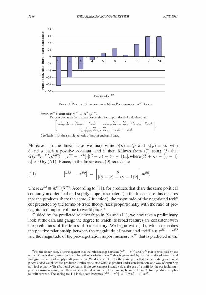
1 2 3 4 5 6 7 8 9 10
Decile of m BR
Figure 1. Percent Deviation from Mean Concession by m BR Decile
notes: mBR is defined as mBR ≡ mBR/pwBR. Percent deviation from mean concession for import decile k calculated as:
[ 1 _ binsize
∑ i∈k ( τ prewto,i − τ wto,i ) − 1 _
10*binsize ∑ k∈10
∑ i∈k
( τ prewto,i − τ wto,i )
_____ | 1 _
10*binsize ∑ k∈10
∑ i∈k
( τ prewto,i − τ wto,i ) |
].
See Table 1 for the sample periods of import and tariff data.
1247BAgWELL And sTAigER: EvidEncE fROm ThE WORLd TRAdE ORgAnizATiOnvOL. 101 nO. 4
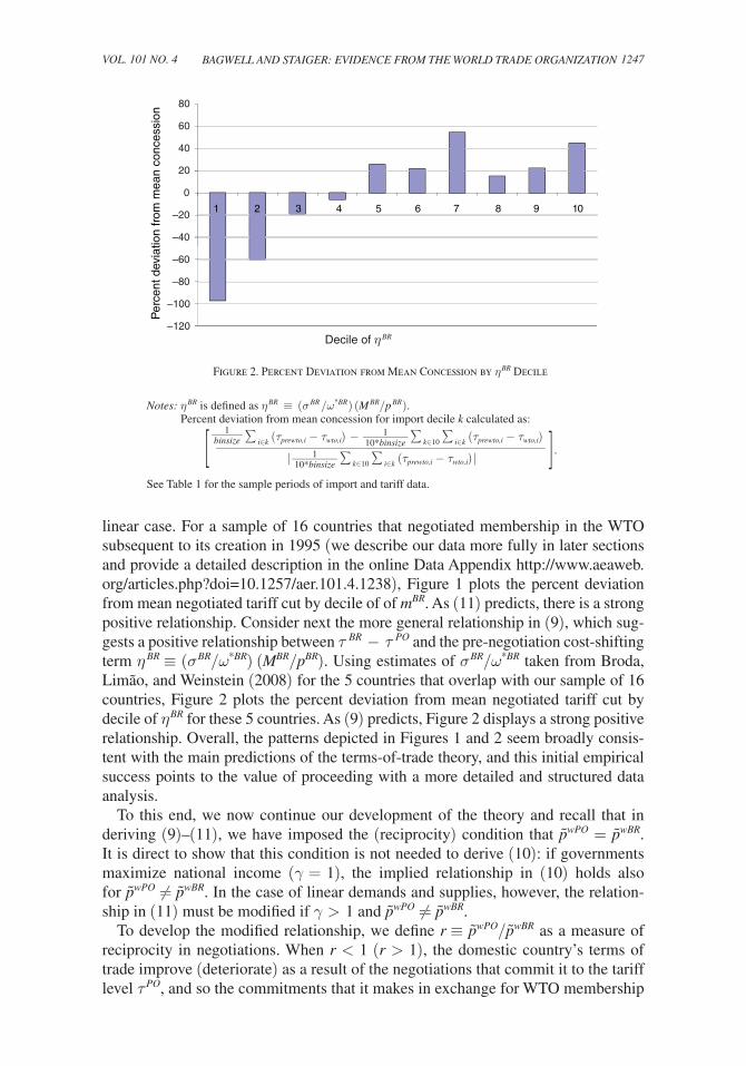
linear case. For a sample of 16 countries that negotiated membership in the WTO subsequent to its creation in 1995 (we describe our data more fully in later sections and provide a detailed description in the online Data Appendix http://www.aeaweb.org/articles.php?doi=10.1257/aer.101.4.1238), Figure 1 plots the percent deviation from mean negotiated tariff cut by decile of of m BR . As (11) predicts, there is a strong positive relationship. Consider next the more general relationship in (9), which sug-gests a positive relationship between τ BR − τ PO and the pre- negotiation cost-shifting term η BR ≡ ( σ BR / ω *BR ) ( m BR / p BR ). Using estimates of σ BR / ω *BR taken from Broda, Limão, and Weinstein (2008) for the 5 countries that overlap with our sample of 16 countries, Figure 2 plots the percent deviation from mean negotiated tariff cut by decile of η BR for these 5 countries. As (9) predicts, Figure 2 displays a strong positive relationship. Overall, the patterns depicted in Figures 1 and 2 seem broadly consis-tent with the main predictions of the terms-of-trade theory, and this initial empirical success points to the value of proceeding with a more detailed and structured data analysis.
To this end, we now continue our development of the theory and recall that in deriving (9)–(11), we have imposed the (reciprocity) condition that p wPO = p wBR . It is direct to show that this condition is not needed to derive (10): if governments maximize national income (γ = 1), the implied relationship in (10) holds also for p wPO ≠ p wBR . In the case of linear demands and supplies, however, the relation-ship in (11) must be modified if γ > 1 and p wPO ≠ p wBR .
To develop the modified relationship, we define r ≡ p wPO / p wBR as a measure of reciprocity in negotiations. When r < 1 (r > 1), the domestic country’s terms of trade improve (deteriorate) as a result of the negotiations that commit it to the tariff level τ PO , and so the commitments that it makes in exchange for WTO membership
–40
–20
0
20
40
60
80
–120
–100
–80
–60
1 2 3 4 5 6 7 8 9 10
Per
cent
dev
iatio
n fr
om m
ean
conc
essi
on
Decile of η BR
Figure 2. Percent Deviation from Mean Concession by ηBR Decile
notes: ηBR is defined as ηBR ≡ (σBR /ω*BR) (mBR/pBR). Percent deviation from mean concession for import decile k calculated as:
[ 1
_ binsize ∑ i∈k ( τ prewto,i − τ wto,i ) − 1 _
10*binsize ∑ k∈10
∑ i∈k
( τ prewto,i − τ wto,i )
_____ | 1 _
10*binsize ∑ k∈10
∑ i∈k
( τ prewto,i − τ wto,i ) |
].
See Table 1 for the sample periods of import and tariff data.

1248 ThE AmERicAn EcOnOmic REviEW JunE 2011
and the rights implied therein are less than (more than) reciprocal in this case. It is now straightforward to show that the generalization of (11) which allows for nonre-ciprocal tariff negotiations (when γ > 1) is given by
τ PO − τ BR = β 0 + ( β 1 − 1) τ BR + β 2 m BR ,
where β 0 = [(γ − 1)κ(r − 1)]/{r[δ + κ − (γ − 1)κ]} with β 0 ⪋ 0 as r ⪋ 1, β 1 = 1/r with β 1 > 0 and β 1 ⪋ 1 as r ⪌ 1, and β 2 = − θ/{r[δ + κ − (γ − 1)κ]} with β 2 < 0, and where we have used [δ + κ − (γ − 1)κ] > 0 under (A1). Finally, rearranging yields
(12) τ PO = β 0 + β 1 τ BR + β 2 m BR .
Hence, under the assumption that demands and supplies are linear, the terms-of-trade theory predicts that estimating a relationship such as (12) on products that share the same political economy and demand and supply slope parameters and the same degree of reciprocity in negotiations would yield an estimated β 1 > 0 and β 2 < 0 (with β 2 → 0 in the limiting case that the country is small in the world market for the products under consideration). That is, as (12) indicates, controlling for the level of the pre-negotiation tariff τ BR , the tariff level τ PO to which a govern-ment commits if negotiations implement the efficient political optimum should be lower the larger is the magnitude of the pre-negotiation import measure m BR .10
More broadly, in the case of general demands and supplies, it is straightfor-ward to show that violations of reciprocity do not upset the basic relationship between τ PO , τ BR , and the pre-negotiation cost-shifting term η BR predicted under reciprocity by (9). Hence, based on the terms-of-trade theory we expect that estimat-ing a relationship of the form
(13) τ PO = ϕ 0 + ϕ 1 τ BR + ϕ 2 η BR
would yield an estimated ϕ 1 > 0 and ϕ 2 < 0; that is, when demands and supplies are nonlinear and controlling for the level of the pre-negotiation tariff τ BR , the tariff level τ PO to which a government commits if negotiations implement the efficient political optimum should be lower the larger is the magnitude of the pre-negotiation cost-shifting term η BR . Equations (12) and (13) form the basis of our empirical anal-ysis in the following sections.
10 In the linear case, we find τ BR = ((γ − 1)[λ + κ p wBR ] + θ m BR )/{[(δ + κ) − (γ − 1)κ] p wBR }. With m BR = [(α − λ) − (δ + κ)(1 + τ BR ) p wBR ], it follows for γ > 1 that changes in the domestic demand and sup-ply shifters α and λ accompanied by changes in foreign demand and supply shifters that fix p wBR and leave τ BR unchanged must change m BR , and (12) then implies that τ PO must change in the opposite direction from the change in m BR . Notice as well from our derivation of (12) that we are not using imports (or import shares, as do Isidro Soloaga, Marcelo Olarreaga, and Winters 1999) to proxy for foreign export supply elasticities, but are rather simply observing that expression (9) takes the form of (12) in the linear (and nonreciprocal) case.
1249BAgWELL And sTAigER: EvidEncE fROm ThE WORLd TRAdE ORgAnizATiOnvOL. 101 nO. 4
II. Empirical Strategy and Data Description
According to the terms-of-trade theory, expressions (12) and (13) predict the out-come of tariff negotiations on the basis of pre-negotiation data. To assess whether these predictions are borne out in the data, our empirical strategy is to estimate equations of the form
(14a) τ gc WTO = β 0 + β 1 τ gc BR + β 2 m gc BR + ϵ gc , and
(14b) τ gc WTO = ϕ 0 + ϕ 1 τ gc BR + ϕ 2 η gc BR + υ gc ,
where g indexes HS six-digit products, c indexes countries, τ gc WTO is the ad valorem tariff level bound by country c on product g in a GATT/WTO negotiation, and ϵ gc and υ gc are error terms.
However, before (14a) and (14b) can be estimated, we must first confront a num-ber of important obstacles. A first obstacle arises because (14a) and (14b) char-acterize a once-for-all movement from unbound (best-response) tariffs to efficient politically optimal tariffs. But GATT/WTO liberalization has occurred very gradu-ally in a series of negotiating rounds that have spanned more than 60 years, with the Uruguay Round (in which the WTO was created) completed at the end of 1994 and marking the eighth and final GATT round.11 This feature precludes a straightforward application of (14a) and (14b) to predict the pattern of GATT/WTO tariff conces-sions across all member countries from data on their pre-GATT tariffs, trade, and elasticity measures. To overcome this, we focus on non-GATT-member countries who joined the WTO in separate accession negotiations occurring after the Uruguay Round was completed. Our maintained hypothesis is that, at the time of these acces-sion negotiations, existing GATT/WTO members had largely completed the pro-cess of negotiating their tariffs to efficient levels, and new members were therefore asked to agree to once-for-all tariff cuts from best-response to politically optimal levels in exchange for the rights of membership.
We acknowledge that this strategy does not come without costs. In particular, we cannot in this paper assess whether the tariff-cutting behavior of the major developed countries, which have historically been the major players in the GATT/WTO sys-tem, conforms with theoretical predictions. Moreover, we are assuming implicitly that the process that led the new-member countries to join the WTO when they did does not introduce important sample selection issues into our subsequent estima-tion. Nevertheless, on balance we believe that the benefits of clear links to the theory outweigh the costs of relatively narrow country coverage, and we leave an empiri-cal evaluation of the tariff-cutting behavior of the broader WTO membership as an important task for future work (on which we comment briefly in the Conclusion).
A second obstacle concerns the measurement of the best-response tariffs. In prin-ciple, τ gc BR can be measured with observations on country c’s tariffs prior to its mem-bership in the WTO. However, when a country joins the WTO it agrees to bring its
11 A first WTO negotiating round, the Doha Round, was initiated in 2001 and is currently ongoing. A number of theories of gradual trade liberalization have been proposed (for a recent example, see Maggi and Rodriguez-Clare 2007), but assessing their empirical implications is beyond the scope of this paper.

1250 ThE AmERicAn EcOnOmic REviEW JunE 2011
“trade regime” into conformity with WTO rules and give up a variety of nontariff forms of trade protection such as quotas and import licensing schemes (see, for example, WTO 2005). The theoretically appropriate measure of τ gc BR would therefore be the ad valorem “tariff equivalent” of a country’s tariff and WTO-inconsistent nontariff measures prior to joining the WTO, but such measures do not exist. We therefore proceed in two steps. For our main results, we utilize a country’s pre-accession ad valorem tariffs as our measure of τ gc BR . But as a robustness check, we also present results supplementing our ad valorem tariff data with the estimates of nontariff barrier (NTB) ad valorem tariff equivalents for 8 of our 16 countries pro-vided by Hiau Looi Kee, Alessandro Nicita, and Olarreaga (2009).12
A third obstacle concerns measures of the trade elasticities σ BR and ω *BR required for the estimation of (14b). In general, such measures are unavailable at a detailed product level. However, Broda, Limão, and Weinstein (2008) have recently pro-vided estimates of these elasticities at the HS four-digit level for 16 countries, 5 of which are also in our dataset.13 In light of the limited availability of these measures, we proceed as follows. For our main results, we focus on the relationship in (14a) where the trade elasticity measures are not required. However, to check the robust-ness of our results, we also present the results from estimating (14b) on a five-country subsample using the Broda, Limão, and Weinstein estimates.
Finally, as (12) indicates, it is important that we carry out our estimation of (14a) in a way that constrains the estimated coefficients to be the same only across prod-ucts that share the same political economy and demand and supply slope param-eters, and the same degree of reciprocity in negotiations; analogous concerns can be expected to apply to our estimation of (14b). For this reason, we present one set of estimates which includes country and industry fixed effects but which con-strains the slope coefficients to be constant across all industries and countries, and we also present a set of estimates for each industrial sector and for each country in the sample so that the slopes may vary across industries or countries, respectively.
Our sample of countries includes 16 of the 21 countries that joined the WTO between its inception on January 1, 1995, and November of 2005.14 Data at the six-digit HS level on each country’s (final) bound ad valorem tariffs, and its pre-WTO-accession (unbound) ad valorem tariffs for an available time period prior to WTO accession, come from the TRAINS dataset. Import data recorded in value terms come from the PC-TAS database (a subset of the COMTRADE database) and are collected at the six-digit HS level and averaged over the years 1995–1999. To convert the PC-TAS import data from value data to quantity data, we utilize unit
12 Kee, Nicita, and Olarreaga (2009) use NTB coverage and frequency data to estimate the import impacts of NTBs in a factor-endowments setting, and construct ad valorem equivalents at the HS six-digit level for 78 countries which include 8 of the 16 countries in our dataset. For our purposes here, these measures are not perfectly defined, as it is not their purpose to discern WTO-inconsistent NTBs from the broader range of NTBs, but they represent the best measures that are available.
13 Broda, Limão, and Weinstein (2008) report elasticity estimates for the United States and for 15 additional countries that were not GATT/WTO members during the time frame used for their analysis. Of these 15 countries, 5 are still nonmembers, while 3 joined GATT prior to the creation of the WTO. Of the remaining 7, two (Saudi Arabia and Taiwan) are excluded from our sample due to issues of data availability (see note 14).
14 The five countries that joined the WTO between January 1, 1995, and November 2005 that are not included in our sample are Bulgaria, Croatia, Taiwan, Mongolia, and Saudi Arabia. These countries were excluded because we could not acquire reliable data on imports and/or unbound tariffs for periods prior to WTO accession.
1251BAgWELL And sTAigER: EvidEncE fROm ThE WORLd TRAdE ORgAnizATiOnvOL. 101 nO. 4
values calculated from the COMTRADE database. A detailed description of all data sources and our data cleaning procedures is contained in the online Data Appendix.
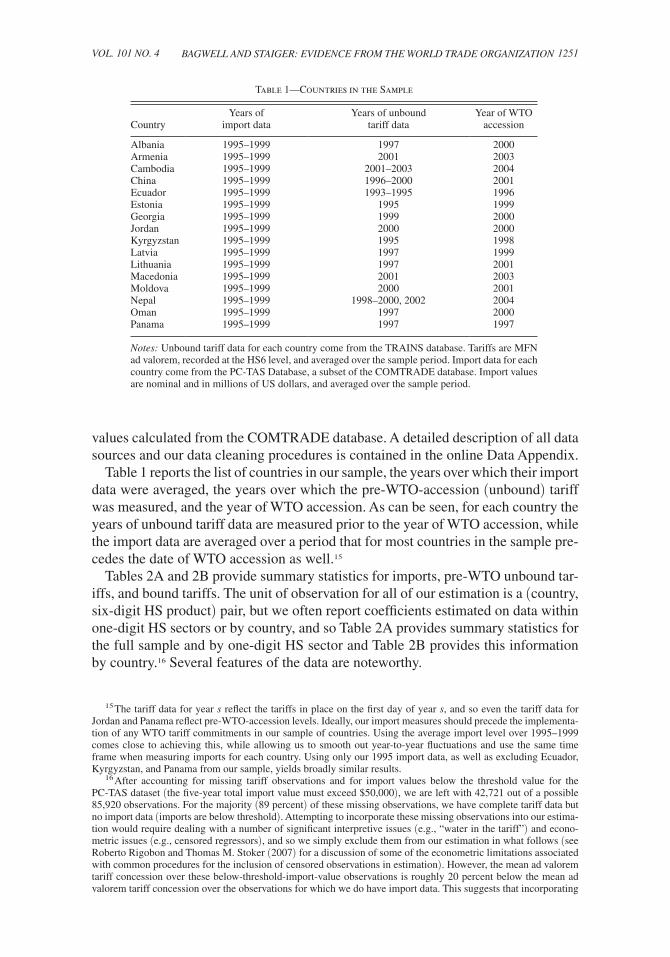
Table 1 reports the list of countries in our sample, the years over which their import data were averaged, the years over which the pre-WTO-accession (unbound) tariff was measured, and the year of WTO accession. As can be seen, for each country the years of unbound tariff data are measured prior to the year of WTO accession, while the import data are averaged over a period that for most countries in the sample pre-cedes the date of WTO accession as well.15
Tables 2A and 2B provide summary statistics for imports, pre-WTO unbound tar-iffs, and bound tariffs. The unit of observation for all of our estimation is a (country, six-digit HS product) pair, but we often report coefficients estimated on data within one-digit HS sectors or by country, and so Table 2A provides summary statistics for the full sample and by one-digit HS sector and Table 2B provides this information by country.16 Several features of the data are noteworthy.
15 The tariff data for year s reflect the tariffs in place on the first day of year s, and so even the tariff data for Jordan and Panama reflect pre-WTO-accession levels. Ideally, our import measures should precede the implementa-tion of any WTO tariff commitments in our sample of countries. Using the average import level over 1995–1999 comes close to achieving this, while allowing us to smooth out year-to-year fluctuations and use the same time frame when measuring imports for each country. Using only our 1995 import data, as well as excluding Ecuador, Kyrgyzstan, and Panama from our sample, yields broadly similar results.
16 After accounting for missing tariff observations and for import values below the threshold value for the PC-TAS dataset (the five-year total import value must exceed $50,000), we are left with 42,721 out of a possible 85,920 observations. For the majority (89 percent) of these missing observations, we have complete tariff data but no import data (imports are below threshold). Attempting to incorporate these missing observations into our estima-tion would require dealing with a number of significant interpretive issues (e.g., “water in the tariff”) and econo-metric issues (e.g., censored regressors), and so we simply exclude them from our estimation in what follows (see Roberto Rigobon and Thomas M. Stoker (2007) for a discussion of some of the econometric limitations associated with common procedures for the inclusion of censored observations in estimation). However, the mean ad valorem tariff concession over these below-threshold-import-value observations is roughly 20 percent below the mean ad valorem tariff concession over the observations for which we do have import data. This suggests that incorporating
Table 1—Countries in the Sample
Years of Years of unbound Year of WTO Country import data tariff data accession
Albania 1995–1999 1997 2000Armenia 1995–1999 2001 2003Cambodia 1995–1999 2001–2003 2004China 1995–1999 1996–2000 2001Ecuador 1995–1999 1993–1995 1996Estonia 1995–1999 1995 1999Georgia 1995–1999 1999 2000Jordan 1995–1999 2000 2000Kyrgyzstan 1995–1999 1995 1998Latvia 1995–1999 1997 1999Lithuania 1995–1999 1997 2001Macedonia 1995–1999 2001 2003Moldova 1995–1999 2000 2001Nepal 1995–1999 1998–2000, 2002 2004Oman 1995–1999 1997 2000Panama 1995–1999 1997 1997
notes: Unbound tariff data for each country come from the TRAINS database. Tariffs are MFN ad valorem, recorded at the HS6 level, and averaged over the sample period. Import data for each country come from the PC-TAS Database, a subset of the COMTRADE database. Import values are nominal and in millions of US dollars, and averaged over the sample period.
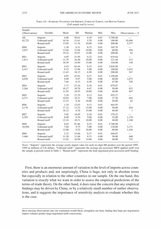
1252 ThE AmERicAn EcOnOmic REviEW JunE 2011
First, there is an enormous amount of variation in the level of imports across coun-tries and products and, not surprisingly, China is huge, not only in absolute terms but especially in relation to the other countries in our sample. On the one hand, this variation is exactly what we want in order to assess the empirical predictions of the terms-of-trade theory. On the other hand, it does raise the concern that any empirical findings may be driven by China, or by a relatively small number of outlier observa-tions, and it suggests the importance of sensitivity analysis to evaluate whether this is the case.
these missing observations into our estimation would likely strengthen our basic finding that large pre-negotiation import volumes predict large negotiated tariff concessions.
Table 2A—Summary Statistics for Imports, Unbound Tariffs, and Bound Tariffs (full sample and by sector)
Sample(Observations) Variable Mean SD Median Min Max Observations = 0
All Imports 4.08 50.61 0.19 0.01 5,788.08 —42,721 Unbound tariff 10.34 11.61 5.70 0.00 180.00 10,496
Bound tariff 13.05 11.34 10.00 0.00 200.00 5,577
HS0 Imports 1.30 6.31 0.15 0.01 165.78 —2,037 Unbound tariff 13.64 12.94 10.00 0.00 60.00 456
Bound tariff 19.32 15.07 15.00 0.00 200.00 83
HS1 Imports 4.05 31.95 0.22 0.01 619.64 —1,811 Unbound tariff 13.79 16.58 10.00 0.00 121.48 413
Bound tariff 18.59 14.89 15.00 0.00 144.00 150
HS2 Imports 4.43 64.44 0.15 0.01 3,826.98 —4,417 Unbound tariff 9.15 13.96 5.00 0.00 180.00 1,033
Bound tariff 11.63 18.15 6.50 0.00 200.00 547
HS3 Imports 4.95 43.91 0.27 0.01 1,190.88 —4,030 Unbound tariff 9.09 9.97 5.00 0.00 60.00 1,073
Bound tariff 7.64 6.33 6.50 0.00 47.00 529
HS4 Imports 3.71 23.34 0.18 0.01 679.07 —3,264 Unbound tariff 10.17 10.70 6.67 0.00 50.00 821
Bound tariff 11.95 10.55 10.00 0.00 40.00 847
HS5 Imports 3.39 27.35 0.12 0.01 955.27 —4,271 Unbound tariff 10.95 10.31 7.00 0.00 37.20 865
Bound tariff 13.33 8.36 10.00 0.00 50.00 82
HS6 Imports 1.24 12.03 0.13 0.01 464.95 —4,176 Unbound tariff 17.12 12.22 15.00 0.00 50.00 654
Bound tariff 18.12 6.76 15.00 0.00 40.00 1
HS7 Imports 3.02 18.05 0.18 0.01 379.22 —4,293 Unbound tariff 8.68 9.70 5.00 0.00 52.00 1,170
Bound tariff 12.16 10.31 10.00 0.00 40.00 1,160
HS8 Imports 6.65 81.86 0.25 0.01 5,788.08 —10,956 Unbound tariff 7.66 9.75 5.00 0.00 130.00 3,171
Bound tariff 12.00 9.22 10.00 0.00 60.00 1,426
HS9 Imports 2.12 15.66 0.17 0.01 440.07 —3,466 Unbound tariff 11.28 11.04 8.33 0.00 50.00 840
Bound tariff 13.62 10.50 14.86 0.00 40.00 752
notes: “Imports’’ represents the average yearly import value for each six-digit HS product over the period 1995–1999 in millions of US dollars. “Unbound tariff’’ represents the average pre-accession MFN applied tariff over the sample at periods noted in Table 1. “Bound tariff’’ represents the final negotiated post-accession tariff binding.

1253BAgWELL And sTAigER: EvidEncE fROm ThE WORLd TRAdE ORgAnizATiOnvOL. 101 nO. 4
Table 2B—Summary Statistics for Imports, Unbound Tariffs, and Bound Tariffs, by Country
Sample(Observations) Variable Mean SD Median Min Max Observations = 0
Albania Imports 0.35 1.45 0.08 0.01 37.24 —2,172 Unbound tariff 16.68 8.74 20.00 0.00 30.00 6
Bound tariff 7.69 6.57 5.00 0.00 20.00 517
Armenia Imports 0.36 2.06 0.06 0.01 42.42 —1,213 Unbound tariff 2.98 4.54 0.00 0.00 10.00 843
Bound tariff 8.66 6.71 10.00 0.00 15.00 402
Cambodia Imports 0.62 4.34 0.08 0.01 153.85 —1,632 Unbound tariff 16.18 12.32 15.00 0.00 96.00 81
Bound tariff 19.33 10.16 15.00 0.00 60.00 13
China Imports 27.96 120.66 3.35 0.01 3,826.98 —4,646 Unbound tariff 18.72 13.03 16.00 0.00 121.48 64
Bound tariff 9.76 6.66 8.50 0.00 65.00 250
Ecuador Imports 1.23 4.63 0.23 0.01 99.48 —3,601 Unbound tariff 11.64 5.71 12.00 0.00 32.33 14
Bound tariff 21.70 7.93 20.00 5.00 85.50 0
Estonia Imports 1.05 4.51 0.25 0.01 171.72 —3,645 Unbound tariff 0.07 0.99 0.00 0.00 16.00 3,625
Bound tariff 8.49 7.59 8.00 0.00 59.00 733
Georgia Imports 0.36 2.40 0.05 0.01 48.29 —1,388 Unbound tariff 9.83 3.24 12.00 5.00 12.00 0
Bound tariff 6.94 5.54 6.50 0.00 30.00 383
Jordan Imports 1.06 5.39 0.19 0.01 204.13 —3,333 Unbound tariff 22.03 14.86 23.33 0.00 180.00 295
Bound tariff 16.05 13.85 15.00 0.00 200.00 206
Kyrgyzstan Imports 0.37 1.73 0.07 0.01 50.09 —1,575 Unbound tariff 0.00 0.00 0.00 0.00 0.00 1,575
Bound tariff 6.99 4.58 10.00 0.00 25.00 365
Latvia Imports 0.83 4.74 0.18 0.01 215.56 —3,253 Unbound tariff 4.78 8.35 0.50 0.00 75.00 131
Bound tariff 12.03 11.83 10.00 0.00 55.00 502
Lithuania Imports 1.30 9.35 0.26 0.01 449.43 —3,515 Unbound tariff 3.62 7.41 0.00 0.00 50.00 2,611
Bound tariff 9.49 7.99 10.00 0.00 100.00 747
Macedonia Imports 0.52 1.94 0.14 0.01 68.21 —2,643 Unbound tariff 14.98 11.42 12.00 0.00 60.00 17
Bound tariff 7.33 7.69 5.75 0.00 60.00 843
Moldova Imports 0.34 3.00 0.07 0.01 118.94 —1,872 Unbound tariff 4.62 5.35 5.00 0.00 16.25 843
Bound tariff 6.94 4.63 7.00 0.00 20.00 383
Nepal Imports 0.41 1.75 0.07 0.01 48.59 —1,517 Unbound tariff 14.89 13.96 15.00 0.00 130.00 40
Bound tariff 25.78 13.99 25.00 0.00 200.00 55
Oman Imports 2.04 11.60 0.19 0.01 290.76 —2,824 Unbound tariff 4.69 1.21 5.00 0.00 5.00 177
Bound tariff 13.23 15.62 15.00 0.00 200.00 85
Panama Imports 3.73 101.05 0.25 0.01 5,788.08 —3,691 Unbound tariff 12.10 11.26 9.00 0.00 60.00 122
Bound tariff 23.36 10.61 30.00 0.00 144.00 75
notes: See Table 2A.

1254 ThE AmERicAn EcOnOmic REviEW JunE 2011
Second, the bound tariffs are generally quite far away from free trade, averaging 13.1 percent across the full sample of products and countries, and ranging across one-digit HS sectors from an average of 7.6 percent to 19.3 percent and across coun-tries from an average of 6.9 percent to 25.8 percent. Indeed, only about 13 percent of the observations on bound tariffs in the full sample of countries and industries correspond to free trade. Hence, predicting the tariff-negotiating outcomes of the WTO does not amount to a trivial exercise of predicting free trade across the board.
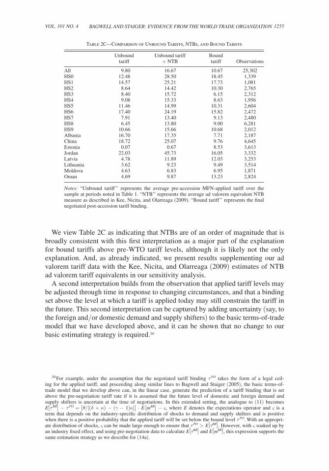
Finally, for many of the countries and industries in the sample, the average bound tariff is higher than the average pre-WTO unbound tariff.17 This may appear to contradict a basic prediction of the terms-of-trade theory, namely, that governments should use international negotiations to lower their tariffs, not raise them, and so it might be tempting to conclude that the theory is refuted by this feature of the data. But this conclusion is not warranted. First, a GATT/WTO binding represents a legal ceiling on the permissible height of a tariff; it does not prevent a government from setting its tariff below the bound level. So this feature of the data does not indicate that governments are using WTO negotiations to raise their tariffs. The real question is whether a WTO binding set above the previously “applied” (unbound) tariff has any effect at all. Certainly governments have traditionally behaved in GATT/WTO negotiations as if they view tariff bindings per se—whether set below, at, or above current applied tariff rates—as having value.18 Here, we offer two interpretations that are consistent with this view, and in each case discuss the implications for the estimation to follow.19
Under a first interpretation, this feature of the data simply reflects the fact that pre-WTO tariffs do not include the protective effects of WTO-inconsistent NTBs which, through the previously described “tariffication” process initiated under WTO acces-sion negotiations, become embodied in the bound rates. To check whether NTBs are large enough to support this interpretation, we utilize the ad valorem equivalent NTB measures generated by Kee, Nicita, and Olarreaga (2009) at the six-digit HS level available for 8 of the 16 countries in our dataset, and incorporate the result-ing tariffication of NTBs into Table 2C. The first column of Table 2C presents the unbound ad valorem tariff, the second column presents the sum of the unbound ad valorem tariff and the ad valorem equivalent NTB measure, and the third column presents the bound ad valorem tariff level. As can be seen, when the ad valorem equivalent NTB measures are added to the ad valorem pre-WTO tariffs, the result-ing tariffied measure of pre-WTO protection is well-above the bound tariff averaged over all countries and industries, and this remains true for the sector-by-sector aver-ages; still, the sum of ad valorem tariff and NTB measures remains below the bound ad valorem tariff for many of the country averages.
17 This is a feature that is shared more generally by many of the developing country members of the WTO, though not by developed country members (see, for example, WTO 2008).
18 See, for example, the discussion in Bernard Hoekman and Michel Kostecki (2001, pp. 130–31) and WTO (2007, p. 192).
19 A number of recent theories provide more complete interpretations, including Bagwell and Staiger (2005), Maggi and Rodriguez-Clare (2007), Bagwell (2009), and Henrik Horn, Maggi, and Staiger (2010). Each of these papers builds from the basic terms-of-trade structure (although Maggi and Rodriguez-Clare introduce commitment issues as well). Rather than develop the specific empirical implications of one of these models, we maintain our general focus and rely on the simple (if less complete) interpretations offered in the text.
1255BAgWELL And sTAigER: EvidEncE fROm ThE WORLd TRAdE ORgAnizATiOnvOL. 101 nO. 4
We view Table 2C as indicating that NTBs are of an order of magnitude that is broadly consistent with this first interpretation as a major part of the explanation for bound tariffs above pre-WTO tariff levels, although it is likely not the only explanation. And, as already indicated, we present results supplementing our ad valorem tariff data with the Kee, Nicita, and Olarreaga (2009) estimates of NTB ad valorem tariff equivalents in our sensitivity analysis.
A second interpretation builds from the observation that applied tariff levels may be adjusted through time in response to changing circumstances, and that a binding set above the level at which a tariff is applied today may still constrain the tariff in the future. This second interpretation can be captured by adding uncertainty (say, to the foreign and/or domestic demand and supply shifters) to the basic terms-of-trade model that we have developed above, and it can be shown that no change to our basic estimating strategy is required.20
20 For example, under the assumption that the negotiated tariff binding τ PO takes the form of a legal ceil-ing for the applied tariff, and proceeding along similar lines to Bagwell and Staiger (2005), the basic terms-of-trade model that we develop above can, in the linear case, generate the prediction of a tariff binding that is set above the pre-negotiation tariff rate if it is assumed that the future level of domestic and foreign demand and supply shifters is uncertain at the time of negotiations. In this extended setting, the analogue to (11) becomes E[ τ BR ] − τ PO = [θ/[(δ + κ) − (γ − 1)κ]] ⋅ E [ m BR ] − ς, where E denotes the expectations operator and ς is a term that depends on the industry-specific distribution of shocks to demand and supply shifters and is positive when there is a positive probability that the applied tariff will be set below the bound level τ PO . With an appropri-ate distribution of shocks, ς can be made large enough to ensure that τ PO > E[ τ BR ]. However, with ς soaked up by an industry fixed effect, and using pre-negotiation data to calculate E[ τ BR ] and E[ m BR ], this expression supports the same estimation strategy as we describe for (14a).
Table 2C—Comparison of Unbound Tariffs, NTBs, and Bound Tariffs
Unboundtariff
Unbound tariff+ NTB
Boundtariff Observations
All 9.80 16.67 10.67 25,302HS0 12.48 28.50 18.45 1,339HS1 14.57 25.21 17.73 1,081HS2 8.64 14.42 10.30 2,765HS3 8.40 15.72 6.15 2,312HS4 9.08 15.33 8.63 1,956HS5 11.46 14.99 10.31 2,604HS6 17.40 24.19 15.82 2,472HS7 7.91 13.40 9.13 2,480HS8 6.45 13.80 9.00 6,281HS9 10.66 15.66 10.68 2,012Albania 16.70 17.35 7.71 2,187China 18.72 25.07 9.76 4,645Estonia 0.07 0.67 8.53 3,613Jordan 22.03 45.73 16.05 3,332Latvia 4.78 11.89 12.03 3,253Lithuania 3.62 9.23 9.49 3,514Moldova 4.63 6.83 6.95 1,871Oman 4.69 9.87 13.23 2,824
notes: “Unbound tariff’’ represents the average pre-accession MFN-applied tariff over the sample at periods noted in Table 1. “NTB’’ represents the average ad valorem equivalent NTB measure as described in Kee, Nicita, and Olarreaga (2009). “Bound tariff’’ represents the final negotiated post-accession tariff binding.
1256 ThE AmERicAn EcOnOmic REviEW JunE 2011
III. Main Results
As developed in the previous sections, the central empirical prediction of the terms-of-trade theory is straightforward: all else equal, the tariff on product g to which country c negotiates should be farther below its noncooperative tariff the larger is the level of country c’s noncooperative import volume (relative to the world price) of product g. Restated in the language of the GATT/WTO, the terms-of-trade theory implies that, all else equal, the magnitude of negotiated tariff concessions should be positively related to pre-negotiation import volumes.
We have already displayed the unconditional relationship between negotiated tariff concessions and pre-negotiation import levels (see Figure 1). As we have noted, the positive relationship displayed by this figure is striking. In fact, this rela-tionship seems so striking that it might be tempting to conclude that a more direct observation can explain it: tariff concessions are big where pre-negotiation import levels are big, because these concessions imply the biggest gains for the foreign exporters whose governments seek the concessions. However, this simple story is too simple, because it ignores the fact that tariff concessions won in a GATT/WTO negotiation do not come “free,” but rather are “purchased” in exchange for recipro-cal concessions. In this light, there is no direct reason why concessions implying big gains for foreign exporters (i.e., where pre-negotiation import levels are big) would be particularly large, since these concessions would carry a reciprocally large negotiating “price” for the governments of the foreign exporters who request them.21 Nevertheless, as we have detailed above, a reason for this relationship is provided by the terms-of-trade theory.22
We next turn to estimation based on (14a). As mentioned, our unit of observation is always a (country, six-digit HS product) pair, but we estimate the following two variants of (14a) on the full sample of countries and products, and on observations grouped by one-digit HS sector and by country:
(15a) τ gc WTO = α g + α c + β 1 τ gc BR + β 2 v gc BR + ϵ gc , and
(15b) τ gc WTO = α g + α c + β 1 τ gc BR + β 2 m gc BR + ϵ gc ,
21 The need to achieve broad reciprocity between rights and obligations is present both in standard market access negotiations in the GATT/WTO and in accession negotiations. For example, the importance of maintaining the balance implied by reciprocity in the context of China’s accession to the WTO was emphasized by the Chinese Delegation: “… a few members have raised some unreasonable requests, either requiring China to undertake obliga-tions exceeding the WTO rules, or insisting that China can not enjoy the rights under the WTO rules. I am deeply concerned with such requests. The balance between rights and obligations is the fundamental principle of China’s WTO accession…” (Long Yongtu 2000). In accession negotiations, which amount to a series of bilateral negotia-tions between each interested member government and the government of the acceding country, each member coun-try typically “pays” for the concessions it wins from the acceding country with its obligation to extend its existing concessions to the new member according to the MFN principle.
22 Of course, it is still possible that the relationship displayed in Figure 1 reflects some simple tariff-cutting rule used by governments rather than the forces indicated by the terms-of-trade theory. It is for this reason that it is important to proceed with a more detailed and structured data analysis on the basis of (14a) and (14b) before draw-ing inferences about the relevance of the terms-of-trade theory for interpreting the data.

1257BAgWELL And sTAigER: EvidEncE fROm ThE WORLd TRAdE ORgAnizATiOnvOL. 101 nO. 4
where α g denotes an industry-fixed effect at the two-digit HS level and α c denotes a country fixed effect.23 The term v gc BR in (15a) denotes import values obtained directly from the PC-TAS database. The term m gc BR in (15b) is constructed by first convert-ing import values v gc BR to import quantities m gc BR using world prices calculated at the two-digit HS level ( m gc BR ≡ v gc BR / p g wBR ), and then dividing m gc BR by p g wBR to arrive at m gc BR ≡ m gc BR / p g wBR . In effect, relative to (14a), (15a) imposes the restriction that world prices do not vary across two-digit HS industries within the relevant sample (so that the world price term can be picked up in the parameter β 2 ), while (15b) employs unit values calculated from the COMTRADE database to relax this restriction.24
The terms-of-trade theory implies that the sign of the estimated parameter β 2 should be negative unless the importing country/countries in the sample are “small” in international markets with respect to the products in the sample, in which case β 2 should be zero. And according to the terms-of-trade theory, β 1 should be positive.
Because our estimation results under (15a) and (15b) are very similar, we present here only our results based on (15a), and include the full set of estimation results in our online Appendix. Table 3A presents our estimates of β 1 and β 2 using OLS and TOBIT.25 The estimates for the full sample are contained in the top row of the table. As can be seen, whether estimated by OLS or TOBIT, the value of β 2 estimated on the full sample is negative and highly significant, providing strong support for the central empirical prediction of the terms-of-trade theory: all else equal, the tariffs to which countries negotiate are further below their noncooperative tariffs the larger are their levels of noncooperative import volumes. This conclusion is further sup-ported with the by-sector results reported in the next ten rows of Table 3A, where for eight out of the ten sectors the OLS estimates of β 2 are negative and significant at the 5 percent level. The TOBIT estimates by sector exhibit higher standard errors, but are still broadly supportive: all point estimates of β 2 are negative, and five of ten are significant at the 5 percent level.26 And as Table 3A indicates, the estimates of β 1 are all highly significant and positive, as the theory would imply.27
23 Using industry fixed effects at the three-, four-, five-, or six-digit HS level makes no material difference to our results. Hence, we present our results here and throughout with two-digit HS level industry fixed effects.
24 We calculate “world” prices as the total value of imports over the 16 sample countries divided by the total quantity of imports over the 16 sample countries, for each two-digit HS industry, averaged over the period 1995–1999. Our results are qualitatively unchanged when world prices are instead calculated at the three-digit HS level, and are somewhat weaker but still broadly supportive of the terms-of-trade theory when world prices are calculated at the four-digit HS level.
25 As mentioned previously, roughly 13 percent of the observations on τ gc WTO in the full sample are zero. This sug-gests that TOBIT estimation may be more appropriate than a linear regression approach, under the assumption that the disturbances in the TOBIT model are normally distributed and homoskedastic. We present both OLS and TOBIT estimates, and emphasize broad findings that are supported by both sets of estimates.
26 Estimates for finer industry-level groupings yield broadly similar results, with no evidence of significantly positive values of β 2 , though some diminishment of the proportion of β 2 estimates that are significantly negative (2/3 when β 2 is estimated separately on observations within each of the 21 HS “sections,” and approximately 1/2 when β 2 is estimated separately on observations within each of the 99 two-digit HS industries). This suggests that the strong within-sector restrictions we impose when reporting our ten by-sector estimates are not driving our results (and when β 2 is estimated separately on observations within two-digit HS industries, a Wald test fails to reject the within-industry restrictions for 95 percent of the industries).
27 Under a strict interpretation of (12), the fact that the estimated β 1 ’s are all less than one could be interpreted as evidence that these countries were asked to make more than reciprocal concessions in exchange for membership in the WTO. However, in our working paper (Bagwell and Staiger 2006) we also develop empirical implications of the commitment theory and show that an estimated β 1 less than one can also be interpreted as evidence of a commitment role of trade agreements. For this reason, we do not emphasize the estimated magnitude of β 1 .

1258 ThE AmERicAn EcOnOmic REviEW JunE 2011
Table 3A—Baseline Results
Equation: τ gc WTO = α g + α c + β 1 τ gc
BR + β 2 [ v gc BR ] + ϵ gc
OLS Tobit
Sample Observations β 1 β 2 R2 β 1 β 2
All 42,721 0.3702*** −0.0044*** 0.804 0.3901*** −0.0065***(0.0174) (0.0008) (0.0051) (0.0010)
HS0 2,037 0.3750*** −0.0733** 0.763 0.3925*** −0.0657(0.0284) (0.0338) (0.0291) (0.0443)
HS1 1,811 0.2226*** −0.0476*** 0.783 0.2376*** −0.0487***(0.0311) (0.0104) (0.0218) (0.0095)
HS2 4,417 0.6502*** −0.0001 0.651 0.6781*** −0.0053(0.0707) (0.0015) (0.0210) (0.0051)
HS3 4,030 0.2679*** −0.0044*** 0.868 0.2805*** −0.0047***(0.0162) (0.0008) (0.0098) (0.0015)
HS4 3,264 0.3285*** −0.0059*** 0.919 0.3711*** −0.0061(0.0142) (0.0017) (0.0147) (0.0048)
HS5 4,271 0.3136*** −0.0055*** 0.955 0.3163*** −0.0055***(0.0104) (0.0015) (0.0083) (0.0020)
HS6 4,176 0.1342*** −0.0134*** 0.974 0.1342*** −0.0134***(0.0144) (0.0044) (0.0089) (0.0041)
HS7 4,293 0.3705*** −0.0111*** 0.906 0.3763*** −0.0088(0.0185) (0.0025) (0.0153) (0.0057)
HS8 10,956 0.4013*** −0.0044*** 0.872 0.4144*** −0.0057***(0.0159) (0.0006) (0.0080) (0.0008)
HS9 3,466 0.3715*** −0.0112* 0.886 0.4123*** −0.0113(0.0176) (0.0063) (0.0179) (0.0082)
Albania 2,172 0.2544*** −0.0085 0.870 0.3194*** −0.0183(0.0208) (0.0512) (0.0256) (0.0690)
Armenia 1,213 0.2693*** 0.0063 0.878 0.3066*** 0.0058(0.0661) (0.0666) (0.0686) (0.0789)
Cambodia 1,632 0.4979*** 0.0453** 0.951 0.4985*** 0.0450(0.0276) (0.0186) (0.0136) (0.0304)
China 4,645 0.2584*** −0.0044*** 0.862 0.2661*** −0.0073***(0.0214) (0.0009) (0.0079) (0.0008)
Ecuador 3,601 0.5703*** −0.0607** 0.972 0.5703*** −0.0607***(0.0224) (0.0244) (0.0182) (0.0146)
Estonia 3,645 0.2124** −0.0900*** 0.870 0.2456* −0.1123***(0.1060) (0.0289) (0.1409) (0.0195)
Georgia 1,388 −0.2285** 0.0457 0.901 −0.4986*** 0.0441(0.0974) (0.0280) (0.1598) (0.0436)
Jordan 3,333 0.6317*** −0.0546** 0.931 0.6504*** −0.0719***(0.0310) (0.0273) (0.0096) (0.0214)
Kyrgyzstan 1,575 — −0.0790 0.904 — −0.0909*— (0.0666) — (0.0506)
Latvia 3,253 0.1246*** −0.0616*** 0.856 0.1286*** −0.1263***(0.0385) (0.0184) (0.0241) (0.0487)
Lithuania 3,515 0.4990*** −0.0051 0.850 0.5179*** −0.0060(0.0445) (0.0115) (0.0223) (0.0110)
Macedonia 2,643 0.4616*** −0.0188 0.859 0.6044*** −0.0183(0.0174) (0.0602) (0.0159) (0.0544)
Moldova 1,872 0.4161*** 0.0009 0.926 0.4755*** 0.0243(0.0329) (0.0031) (0.0252) (0.1509)
Nepal 1,517 0.3516*** −0.3998** 0.941 0.3527*** −0.4073***(0.0391) (0.1810) (0.0183) (0.1150)
Oman 2,824 −0.4555 −0.0248** 0.765 −0.4662** −0.0258(0.5301) (0.0124) (0.2351) (0.0174)
Panama 3,691 0.1277*** −0.0031*** 0.925 0.1300*** −0.0032**(0.0179) (0.0010) (0.0132) (0.0012)
notes: Standard errors are in parentheses (OLS are heteroskedasticity-robust). Industry fixed effects, α g , are at the two-digit HS product level. Country fixed effects, α c , included only for the full-sample and by-sector estimates. Fixed-effect estimates available upon request. See main text for variable definitions.
*** Significant at the 1 percent level. ** Significant at the 5 percent level. * Significant at the 10 percent level.
1259BAgWELL And sTAigER: EvidEncE fROm ThE WORLd TRAdE ORgAnizATiOnvOL. 101 nO. 4
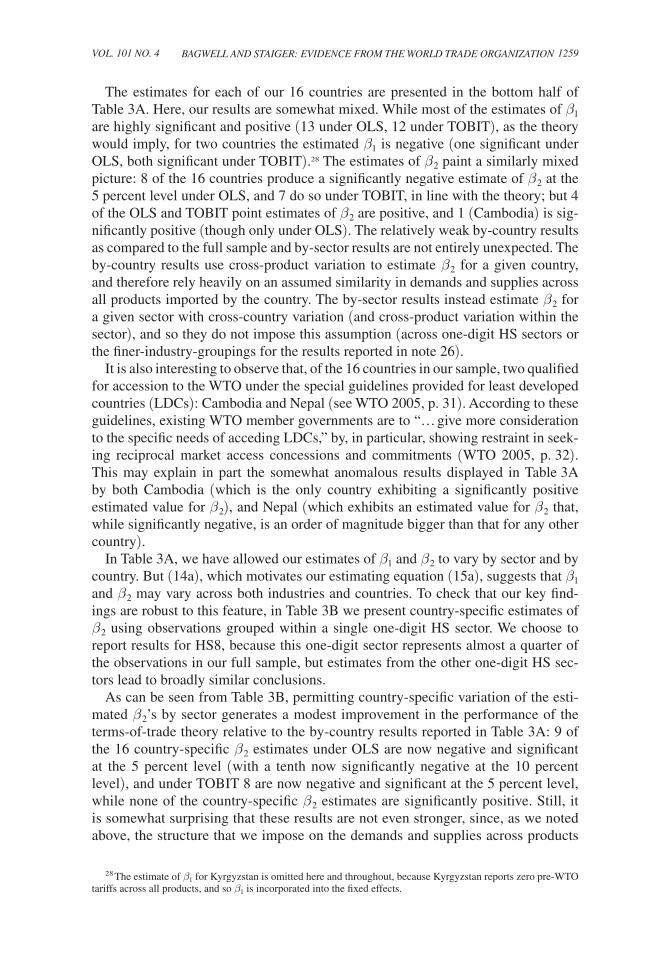
The estimates for each of our 16 countries are presented in the bottom half of Table 3A. Here, our results are somewhat mixed. While most of the estimates of β 1 are highly significant and positive (13 under OLS, 12 under TOBIT), as the theory would imply, for two countries the estimated β 1 is negative (one significant under OLS, both significant under TOBIT).28 The estimates of β 2 paint a similarly mixed picture: 8 of the 16 countries produce a significantly negative estimate of β 2 at the 5 percent level under OLS, and 7 do so under TOBIT, in line with the theory; but 4 of the OLS and TOBIT point estimates of β 2 are positive, and 1 (Cambodia) is sig-nificantly positive (though only under OLS). The relatively weak by-country results as compared to the full sample and by-sector results are not entirely unexpected. The by-country results use cross-product variation to estimate β 2 for a given country, and therefore rely heavily on an assumed similarity in demands and supplies across all products imported by the country. The by-sector results instead estimate β 2 for a given sector with cross-country variation (and cross-product variation within the sector), and so they do not impose this assumption (across one-digit HS sectors or the finer-industry-groupings for the results reported in note 26).
It is also interesting to observe that, of the 16 countries in our sample, two qualified for accession to the WTO under the special guidelines provided for least developed countries (LDCs): Cambodia and Nepal (see WTO 2005, p. 31). According to these guidelines, existing WTO member governments are to “… give more consideration to the specific needs of acceding LDCs,” by, in particular, showing restraint in seek-ing reciprocal market access concessions and commitments (WTO 2005, p. 32). This may explain in part the somewhat anomalous results displayed in Table 3A by both Cambodia (which is the only country exhibiting a significantly positive estimated value for β 2 ), and Nepal (which exhibits an estimated value for β 2 that, while significantly negative, is an order of magnitude bigger than that for any other country).
In Table 3A, we have allowed our estimates of β 1 and β 2 to vary by sector and by country. But (14a), which motivates our estimating equation (15a), suggests that β 1 and β 2 may vary across both industries and countries. To check that our key find-ings are robust to this feature, in Table 3B we present country-specific estimates of β 2 using observations grouped within a single one-digit HS sector. We choose to report results for HS8, because this one-digit sector represents almost a quarter of the observations in our full sample, but estimates from the other one-digit HS sec-tors lead to broadly similar conclusions.
As can be seen from Table 3B, permitting country-specific variation of the esti-mated β 2 ’s by sector generates a modest improvement in the performance of the terms-of-trade theory relative to the by-country results reported in Table 3A: 9 of the 16 country-specific β 2 estimates under OLS are now negative and significant at the 5 percent level (with a tenth now significantly negative at the 10 percent level), and under TOBIT 8 are now negative and significant at the 5 percent level, while none of the country-specific β 2 estimates are significantly positive. Still, it is somewhat surprising that these results are not even stronger, since, as we noted above, the structure that we impose on the demands and supplies across products
28 The estimate of β 1 for Kyrgyzstan is omitted here and throughout, because Kyrgyzstan reports zero pre-WTO tariffs across all products, and so β 1 is incorporated into the fixed effects.
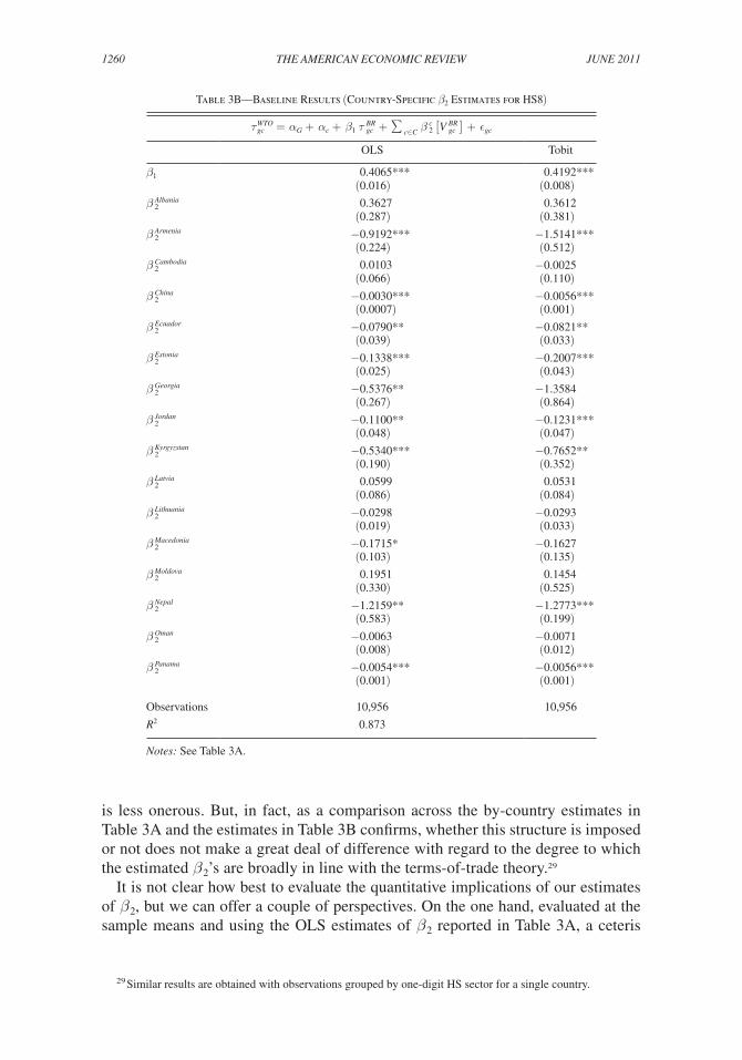
1260 ThE AmERicAn EcOnOmic REviEW JunE 2011
is less onerous. But, in fact, as a comparison across the by-country estimates in Table 3A and the estimates in Table 3B confirms, whether this structure is imposed or not does not make a great deal of difference with regard to the degree to which the estimated β 2 ’s are broadly in line with the terms-of-trade theory.29
It is not clear how best to evaluate the quantitative implications of our estimates of β 2 , but we can offer a couple of perspectives. On the one hand, evaluated at the sample means and using the OLS estimates of β 2 reported in Table 3A, a ceteris
29 Similar results are obtained with observations grouped by one-digit HS sector for a single country.
Table 3B—Baseline Results (Country-Specific β 2 Estimates for HS8)
τ gc WTO = α g + α c + β 1 τ gc
BR + ∑ c∈c β 2
c [ v gc
BR ] + ϵ gc
OLS Tobit
β 1 0.4065*** 0.4192***(0.016) (0.008)
β 2 Albania 0.3627 0.3612
(0.287) (0.381) β 2
Armenia −0.9192*** −1.5141***(0.224) (0.512)
β 2 cambodia 0.0103 −0.0025
(0.066) (0.110) β 2
china −0.0030*** −0.0056***(0.0007) (0.001)
β 2 Ecuador −0.0790** −0.0821**
(0.039) (0.033) β 2
Estonia −0.1338*** −0.2007***(0.025) (0.043)
β 2 georgia −0.5376** −1.3584
(0.267) (0.864) β 2
Jordan −0.1100** −0.1231***(0.048) (0.047)
β 2 Kyrgyzstan −0.5340*** −0.7652**
(0.190) (0.352) β 2
Latvia 0.0599 0.0531(0.086) (0.084)
β 2 Lithuania −0.0298 −0.0293
(0.019) (0.033) β 2
macedonia −0.1715* −0.1627(0.103) (0.135)
β 2 moldova 0.1951 0.1454
(0.330) (0.525) β 2
nepal −1.2159** −1.2773***(0.583) (0.199)
β 2 Oman −0.0063 −0.0071
(0.008) (0.012) β 2
Panama −0.0054*** −0.0056***(0.001) (0.001)
Observations 10,956 10,956
R2 0.873
notes: See Table 3A.

1261BAgWELL And sTAigER: EvidEncE fROm ThE WORLd TRAdE ORgAnizATiOnvOL. 101 nO. 4
paribus increase in noncooperative imports by one standard deviation is predicted to lower bound tariff levels by about 1.7 percent based on the full sample (which at the mean full-sample binding is less than 1/4 of a percentage point), and never as high as 10 percent for any industry or country subsample. This seems rather small. On the other hand, the β 2 estimate for China implies that a ceteris paribus increase in the noncooperative imports for China by one standard deviation is predicted to lower China’s bound tariff levels by about 5.5 percent (which at the mean China binding is a little over 1/2 of a percentage point), and this is an effect that is larger than that implied for any other country in our sample. Analogous conclusions follow from our TOBIT estimates of β 2 . Hence, the quantitative implications of our estimates of β 2 are sometimes sizeable, and they are biggest for countries that are by any metric “large” in world markets.
This conclusion is reinforced from a different perspective. Provided that γ is suf-ficiently close to one, so that governments in our sample behave in a fashion that is not too far from national income maximization, and provided that r is sufficiently similar across countries, so that these countries were asked to make concessions in exchange for WTO membership which implied a similar level of reciprocity, the estimated β 2 ’s can be used to construct an implied ranking over countries of the foreign export supply elasticities ω *BR faced by importers when evaluated at sample means.30 Using again the OLS estimates of β 2 by country reported in Table 3A, the implied ranking of ω *BR across importing countries puts China second from the bottom of the list (and at the bottom of the list if Nepal is excluded as “anoma-lous” according to the logic described above); and under the TOBIT estimates of β 2 reported in Table 3A China faces the lowest value of ω *BR among all importing countries in our sample.
In fact, the rank correlation between the implied 1/ ω *BR faced by a country and that country’s average GDP over the 1995–1999 period is 0.58 when the OLS esti-mates of β 2 are used and Nepal and Cambodia are excluded as “anomalous,” and is 0.50 when the TOBIT estimates of β 2 are used instead. These findings are consistent with the broadly held intuition that international market power is positively related to country size, an intuition that also finds empirical support in the work of Broda, Limão, and Weinstein (2008). Moreover, for the subsample of five countries that are in the Broda, Limão, and Weinstein dataset and also in ours, the correlation between the ranking of our implied country-level 1/ ω *BR and their median estimated 1/ ω *BR by country is 0.9 when the OLS estimates of β 2 are used, and 0.7 when the TOBIT estimates of β 2 are used.
Our estimated β 2 ’s can also be used to construct an implied ranking over indus-tries of the value of ω *BR faced by importers when evaluated at sample means. Using the OLS estimates of β 2 reported in Table 3A, the implied ranking of ω *BR across one-digit HS sectors identifies HS0 and HS1, where animal and vegetable products figure prominently, as the sectors exhibiting the lowest levels of ω *BR . The next low-est levels of ω *BR are found in HS7, HS8, and HS9, which are sectors dominated
30 To see this, note using (12), (15a), and the definition of θ that − β 2 _
v BR = (δ + κ)/{r[(δ + κ) − (γ − 1)κ]}(1/ _ ω *BR ), where
_ v BR and
_ ω *BR denote magnitudes evaluated at sample means. Hence, if (γ − 1) is small
and r is similar across observations, then the ranking of −1/ β 2 v− BR preserves the ranking of
_ ω *BR .

1262 ThE AmERicAn EcOnOmic REviEW JunE 2011
by manufacturing products. And the highest level of ω *BR is found in HS2, which is dominated by mineral products and chemicals.
It is somewhat surprising (and at odds with the results of Broda, Limão, and Weinstein 2008) that the animal and vegetable product sectors HS0 and HS1, rather than the manufacturing sectors HS7-9, exhibit the lowest foreign export supply elasticities. But this broad pattern is preserved when we refine (not shown) our by-sector estimates to the 21 HS sections that are designed to more accurately group together goods produced in the same sector of the economy. And when we generate by-sector estimates for each country and perform the calculations above, a similar pattern emerges. So while our results point to manufacturing goods as exhibiting relatively low foreign export sup-ply elasticities and mineral and chemical products as exhibiting relatively high foreign export supply elasticities, they also strongly indicate that animal and vegetable prod-ucts are among the lowest foreign export supply elasticity sectors.31
Thus far, we have proceeded according to the view that the foreign exporters sell-ing m gc BR of product g into acceding country c’s market are all located in countries that are existing WTO members, so that their governments can internalize through accession negotiations the terms-of-trade externality that country c imposes with its tariff on product g. While this view is approximately borne out in our data, it is not literally true: the fraction of acceding country imports that are supplied by existing WTO members is less than one for about 25 percent of the observations in our full sample. This suggests an opportunity to explore whether the effects we have identi-fied are found only where we would expect to find them. We thus wish to explore the possibility that τ gc WTO is higher when the fraction of country c’s pre-negotiation imports of product g supplied by non-WTO members is higher.
To capture this possibility, we first define O gc BR as the value of country c’s pre-negotiation imports of product g supplied by “outsiders,” i.e., non-WTO members. We then extend our estimating equations and estimate the following variants of (15a) and (15b) on the full sample of countries and products, and on observations grouped by one-digit HS sector and by country:
(16a) τ gc WTO = α g + α c + β 1 τ gc BR + β 2 v gc BR + β 3 O gc BR + ϵ gc , and
(16b) τ gc WTO = α g + α c + β 1 τ gc BR + β 2 m gc BR + β 3 o gc BR + ϵ gc ,
where the term o gc BR in (16b) is constructed by first converting O gc BR to a quantity mea-sure using p g wBR and then dividing this quantity measure by p g wBR . As with (15a) and (15b), relative to (14a), (16a) imposes the restriction that world prices do not vary across two-digit HS industries within the relevant sample (so that the world price
31 A possible interpretation of this finding is that the markets for animal/vegetable products are more regional (reflecting, perhaps, the perishable nature of these products) than the markets for mineral/chemical products. Indeed, our theory implies that, all else equal,
_ ω *BR is smaller when an importing country is served by fewer export-
ing countries and competes with fewer importing countries. As a rough check, we calculate at the six-digit HS product level the trade-weighted average numbers of export-source countries and of competing importer countries, and find that the average number of competing importer countries and export-source countries is 6 percent lower and 48 percent lower, respectively, for animal/vegetable products as compared to mineral/chemical products, in line with this interpretation. We note as well that this interpretation is consistent with the general finding of Broda, Limão, and Weinstein (2008) that more remote countries have greater market power.
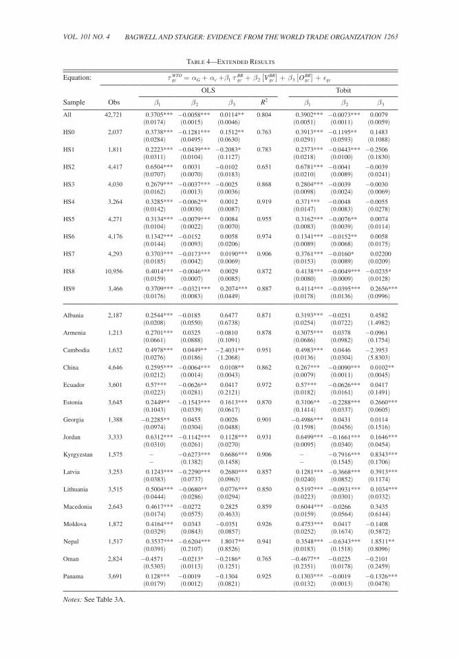
1263BAgWELL And sTAigER: EvidEncE fROm ThE WORLd TRAdE ORgAnizATiOnvOL. 101 nO. 4
Table 4—Extended Results
Equation: τ gc WTO = α g + α c + β 1 τ gc
BR + β 2 [ v gc BR ] + β 3 [ O gc
BR ] + ϵ gc
OLS Tobit
Sample Obs β 1 β 2 β 3 R2 β 1 β 2 β 3
All 42,721 0.3705*** −0.0058*** 0.0114** 0.804 0.3902*** −0.0073*** 0.0079(0.0174) (0.0015) (0.0046) (0.0051) (0.0011) (0.0059)
HS0 2,037 0.3738*** −0.1281*** 0.1512** 0.763 0.3913*** −0.1195** 0.1483(0.0284) (0.0495) (0.0630) (0.0291) (0.0593) (0.1088)
HS1 1,811 0.2223*** −0.0439*** −0.2083* 0.783 0.2373*** −0.0443*** −0.2506(0.0311) (0.0104) (0.1127) (0.0218) (0.0100) (0.1830)
HS2 4,417 0.6504*** 0.0031 −0.0102 0.651 0.6781*** −0.0041 −0.0039(0.0707) (0.0070) (0.0183) (0.0210) (0.0089) (0.0241)
HS3 4,030 0.2679*** −0.0037*** −0.0025 0.868 0.2804*** −0.0039 −0.0030(0.0162) (0.0013) (0.0036) (0.0098) (0.0024) (0.0069)
HS4 3,264 0.3285*** −0.0062** 0.0012 0.919 0.371*** −0.0048 −0.0055(0.0142) (0.0030) (0.0087) (0.0147) (0.0083) (0.0278)
HS5 4,271 0.3134*** −0.0079*** 0.0084 0.955 0.3162*** −0.0076** 0.0074(0.0104) (0.0022) (0.0070) (0.0083) (0.0039) (0.0114)
HS6 4,176 0.1342*** −0.0152 0.0058 0.974 0.1341*** −0.0152** 0.0058(0.0144) (0.0093) (0.0206) (0.0089) (0.0068) (0.0175)
HS7 4,293 0.3703*** −0.0173*** 0.0190*** 0.906 0.3761*** −0.0160* 0.02200(0.0185) (0.0042) (0.0069) (0.0153) (0.0089) (0.0209)
HS8 10,956 0.4014*** −0.0046*** 0.0029 0.872 0.4138*** −0.0049*** −0.0235*(0.0159) (0.0007) (0.0085) (0.0080) (0.0009) (0.0128)
HS9 3,466 0.3709*** −0.0321*** 0.2074*** 0.887 0.4114*** −0.0395*** 0.2656***(0.0176) (0.0083) (0.0449) (0.0178) (0.0136) (0.0996)
Albania 2,187 0.2544*** −0.0185 0.6477 0.871 0.3193*** −0.0251 0.4582(0.0208) (0.0550) (0.6738) (0.0254) (0.0722) (1.4982)
Armenia 1,213 0.2701*** 0.0325 −0.0810 0.878 0.3075*** 0.0378 −0.0961(0.0661) (0.0888) (0.1091) (0.0686) (0.0982) (0.1754)
Cambodia 1,632 0.4978*** 0.0449** −2.4031** 0.951 0.4983*** 0.0446 −2.3953(0.0276) (0.0186) (1.2068) (0.0136) (0.0304) (5.8303)
China 4,646 0.2595*** −0.0064*** 0.0108** 0.862 0.267*** −0.0090*** 0.0102**(0.0212) (0.0014) (0.0043) (0.0079) (0.0011) (0.0045)
Ecuador 3,601 0.57*** −0.0626** 0.0417 0.972 0.57*** −0.0626*** 0.0417(0.0223) (0.0281) (0.2121) (0.0182) (0.0161) (0.1491)
Estonia 3,645 0.2449** −0.1543*** 0.1613*** 0.870 0.3106** −0.2288*** 0.2660***(0.1043) (0.0339) (0.0617) (0.1414) (0.0337) (0.0605)
Georgia 1,388 −0.2285** 0.0455 0.0026 0.901 −0.4986*** 0.0431 0.0114(0.0974) (0.0304) (0.0488) (0.1598) (0.0456) (0.1516)
Jordan 3,333 0.6312*** −0.1142*** 0.1128*** 0.931 0.6499*** −0.1661*** 0.1646***(0.0310) (0.0261) (0.0270) (0.0095) (0.0340) (0.0454)
Kyrgyzstan 1,575 − −0.6273*** 0.6686*** 0.906 − −0.7916*** 0.8343***− (0.1382) (0.1458) − (0.1545) (0.1706)
Latvia 3,253 0.1243*** −0.2290*** 0.2680*** 0.857 0.1281*** −0.3668*** 0.3913***(0.0383) (0.0737) (0.0963) (0.0240) (0.0852) (0.1174)
Lithuania 3,515 0.5004*** −0.0680** 0.0776*** 0.850 0.5197*** −0.0931*** 0.1034***(0.0444) (0.0286) (0.0294) (0.0223) (0.0301) (0.0332)
Macedonia 2,643 0.4617*** −0.0272 0.2825 0.859 0.6044*** −0.0266 0.3435(0.0174) (0.0575) (0.4633) (0.0159) (0.0564) (0.6144)
Moldova 1,872 0.4164*** 0.0343 −0.0351 0.926 0.4753*** 0.0417 −0.1408(0.0329) (0.0843) (0.0857) (0.0252) (0.1674) (0.5872)
Nepal 1,517 0.3537*** −0.6204*** 1.8017** 0.941 0.3548*** −0.6343*** 1.8511**(0.0391) (0.2107) (0.8526) (0.0183) (0.1518) (0.8096)
Oman 2,824 −0.4571 −0.0213* −0.2186* 0.765 −0.4677** −0.0225 −0.2101(0.5303) (0.0113) (0.1251) (0.2351) (0.0178) (0.2459)
Panama 3,691 0.128*** −0.0019 −0.1304 0.925 0.1303*** −0.0019 −0.1326***(0.0179) (0.0012) (0.0821) (0.0132) (0.0013) (0.0478)
notes: See Table 3A.
1264 ThE AmERicAn EcOnOmic REviEW JunE 2011
term can be picked up in the estimated parameters), while (16b) employs unit val-ues calculated from the COMTRADE data base to relax this restriction. We expect the sign of β 2 to be negative and the sign of β 3 to be positive unless the importing country/countries in the sample are “small” in international markets with respect to the industry/industries in the sample (in which case β 2 and β 3 should be zero), and we expect the sign of β 1 to be positive.
Again, because our estimation results under (16a) and (16b) are very similar, we present here only our results based on (16a), and include the full set of estimation results in our online Appendix. Table 4 presents our estimates of β 1 , β 2 , and β 3 using OLS and TOBIT. The first row presents the estimates for the full sample. The OLS estimates perform exactly as the terms-of-trade theory would predict: greater imports from nonmember countries lead to significantly higher bound tariffs (the estimated β 3 is positive and highly significant), and taking account of this increases somewhat the estimated magnitude of β 2 (which is again negative and highly significant). The TOBIT point estimate of β 3 is positive as well, although it is not significant. The next 10 rows of Table 4 present the results by sector. Most of the ten by-sector point estimates of β 3 are positive, and are significantly positive for three sectors under OLS and one sector under TOBIT (one estimated β 3 under both OLS and TOBIT is sig-nificantly negative at the 10 percent level, though none is significantly negative at the 5 percent level). The estimates of β 2 are not much affected, though it is encouraging that now an additional sector under TOBIT yields a significantly negative β 2 estimate at the 5 percent level (with a second additional sector now yielding a significantly negative estimate of β 2 at the 10 percent level). The by-country estimates in Table 4 are also somewhat encouraging. Most of the by-country point estimates of β 3 are positive, and are significantly positive for 7 of the 16 countries under both OLS and TOBIT (under both OLS and TOBIT, 1 estimated β 3 is significantly negative at the 5 percent level, while under OLS an additional estimated β 3 is significantly negative at the 10 percent level). The by-country estimates of β 2 are slightly more support-ive of the terms-of-trade theory when the outsider variable O gc BR is included, with an additional OLS estimate of β 2 now significantly negative at the 10 percent level and an additional TOBIT estimate of β 2 now significantly negative at the 5 percent level.
Overall, the baseline estimation results presented in Tables 3 and 4 confirm what is suggested by Figure 1, and indicate a broad level of support for the central pre-dictions of the terms-of-trade theory. And the effects appear to be most pronounced primarily where we would expect to find them, namely, where the importer is “large” by any measure and where import volume is supplied by current WTO members.
IV. Robustness
In this section we explore the robustness of the main findings reported in the pre-vious section. We first augment our measure of the noncooperative best-response tariff τ gc BR . In particular, supplementing our ad valorem tariff data with the NTB ad valorem–equivalent measures reported in Kee, Nicita, and Olarreaga (2009) for 8 of our 16 countries (see note 12), we reestimate (15a) and (15b) using this subsample of 8 countries with τ gc BR measured by the sum of the pre-WTO ad valorem tariff and the Kee, Nicita, and Olarreaga NTB ad valorem–equivalent measures. Tables 5A and 5B present the results of this reestimation for (15a) using OLS and TOBIT (the

1265BAgWELL And sTAigER: EvidEncE fROm ThE WORLd TRAdE ORgAnizATiOnvOL. 101 nO. 4
results for (15b) are similar and can be found in our online Appendix). Table 5A presents the estimates for the full (sub) sample and by sector and by country; Table 5B presents the estimates by country for the one-digit HS sector 8. Comparing the results reported in Tables 5A–5B with those in Tables 3A–3B, the pattern and strength of our earlier findings are preserved under our augmented measure of pre-WTO-accession protection levels (and, if anything, the support for the terms-of-trade theory is slightly stronger), and it is also reassuring that the magni-tudes of the estimated β 2 ’s do not change significantly.
Table 5A—Sensitivity Analysis: NTB Measures
Equation: τ gc WTO = α g + α c + β 1 ( τ gc
BR + nTB gc ) + β 2 [ v gc BR ] + ϵ gc
OLS Tobit
Sample Obs β 1 β 2 R2 β 1 β 2
All 25,302 0.0459*** −0.0037*** 0.684 0.0474*** −0.0070***(0.0040) (0.0008) (0.0023) (0.0015)
HS0 1,339 0.0091 −0.0858** 0.703 0.0098 −0.0800(0.0143) (0.0378) (0.0113) (0.0493)
HS1 1,081 0.0278** −0.0186*** 0.728 0.0298*** −0.0178*(0.0115) (0.0052) (0.0111) (0.0104)
HS2 2,765 0.0768** −0.0014 0.479 0.0732*** −0.0088(0.0319) (0.0012) (0.0131) (0.0074)
HS3 2,312 0.0059** −0.0049*** 0.859 0.0052** −0.0053***(0.0028) (0.0010) (0.0025) (0.0011)
HS4 1,956 0.03*** −0.0095*** 0.844 0.0276*** −0.0102**(0.0070) (0.0024) (0.0059) (0.0050)
HS5 2,604 0.0461*** −0.0062*** 0.902 0.0461*** −0.0062***(0.0069) (0.0017) (0.0036) (0.0021)
HS6 2,472 0.0051* −0.0105*** 0.971 0.0051** −0.0105***(0.0029) (0.0035) (0.0025) (0.0037)
HS7 2,480 0.0321*** −0.0156*** 0.812 0.0383*** −0.0135**(0.0073) (0.0036) (0.0066) (0.0064)
HS8 6,281 0.0447*** −0.0042*** 0.747 0.0459*** −0.0071***(0.0049) (0.0010) (0.0034) (0.0015)
HS9 2,012 0.0172** −0.0117** 0.788 0.015* −0.0131(0.0083) (0.0054) (0.0079) (0.0093)
Albania 2,187 0.0666*** −0.0152 0.863 0.1222*** −0.022(0.0219) (0.0593) (0.0153) (0.0705)
China 4,645 0.0302*** −0.0042*** 0.831 0.0314*** −0.0068***(0.0041) (0.0008) (0.0028) (0.0009)
Estonia 3,613 −0.0028 −0.0856*** 0.869 −0.0037 −0.1068***(0.0066) (0.0271) (0.0131) (0.0193)
Jordan 3,332 0.0448*** −0.0920*** 0.837 0.0456*** −0.1105***(0.0057) (0.0345) (0.0040) (0.0329)
Latvia 3,253 0.0206** −0.0614*** 0.855 0.0225*** −0.1330***(0.0088) (0.0193) (0.0057) (0.0500)
Lithuania 3,514 0.0298*** −0.0039 0.822 0.0322*** −0.0047(0.0051) (0.0107) (0.0052) (0.0120)
Moldova 1,871 0.0010 −0.0026 0.911 −0.0013 −0.1694(0.0041) (0.0041) (0.0060) (0.1658)
Oman 2,824 −0.0479** −0.0241** 0.766 −0.0497*** −0.0250(0.0191) (0.0123) (0.0113) (0.0173)
notes: See Table 3A.

1266 ThE AmERicAn EcOnOmic REviEW JunE 2011
Next, as noted in Section II, our dataset contains a number of observations with very large import values. To address the possibility that import outliers could be dominating our results, we estimate (15a) in semi-log form according to
τ gc WTO = α g + α c + β 1 τ gc BR + β 2 [ln( v gc BR )] + ϵ gc .
The top half of Table 5C presents the estimation results for the full sample and on observations grouped by one-digit HS sector, while the bottom half of Table 5C presents the results based on observations grouped by country. As can be seen, the semi-log specification, if anything, provides stronger support for the terms-of-trade theory. The full-sample and by-sector OLS and TOBIT estimates of β 2 continue to be strongly supportive of the theory, with TOBIT estimates of β 2 now significantly negative at the 5 percent level for eight of the sectors (and significantly negative for the remaining two sectors at the 10 percent level), in line with the OLS estimates. And now 11 of the 16 by-country estimates of β 2 under both OLS and TOBIT are significantly negative at the 5 percent level, with only two positive OLS point esti-mates and none significantly positive (the estimates of β 1 are little changed).32
32 In our online Appendix, we also report the results of reestimating (15a) with China excluded, and with China included but with Chinese “processing imports” excluded (we thank Robert Feenstra for providing us with the data with which to calculate the breakdown between processing and normal imports for China). The results provide roughly the same level of support for the terms-of-trade theory that our main results indicate. And as a further check on the robustness of our results with regard to import outliers, we also reran our estimation on a sample that excluded observations with import values below various cutoff levels, on the grounds that low reported import values are often thought to be highly unreliable, with essentially no change in the results.
Table 5B—Sensitivity Analysis: NTB Measures (Country−Specific β 2 Estimates for hs8)
τ gc WTO = α g + α c + β 1 ( τ gc
BR + nTB gc ) + ∑ c∈c β 2
c [ v gc
BR ] + ϵ gc
OLS Tobit
β 1 0.0445*** 0.0457***(0.005) (0.003)
β 2 Albania 0.4044 0.4167
(0.372) (0.397) β 2
china −0.0039*** −0.0066***(0.001) (0.001)
β 2 Estonia −0.1326*** −0.2018***
(0.029) (0.044) β 2
Jordan −0.0723 −0.0807*(0.059) (0.049)
β 2 Latvia −0.0440 −0.0590
(0.072) (0.088) β 2
Lithuania −0.0563* −0.0557(0.029) (0.034)
β 2 moldovia 0.0185 −0.0369
(0.389) (0.547) β 2
Oman −0.0144** −0.0155(0.007) (0.012)
Observations 6,281 6,281
R2 0.747
notes: See Table 3A.
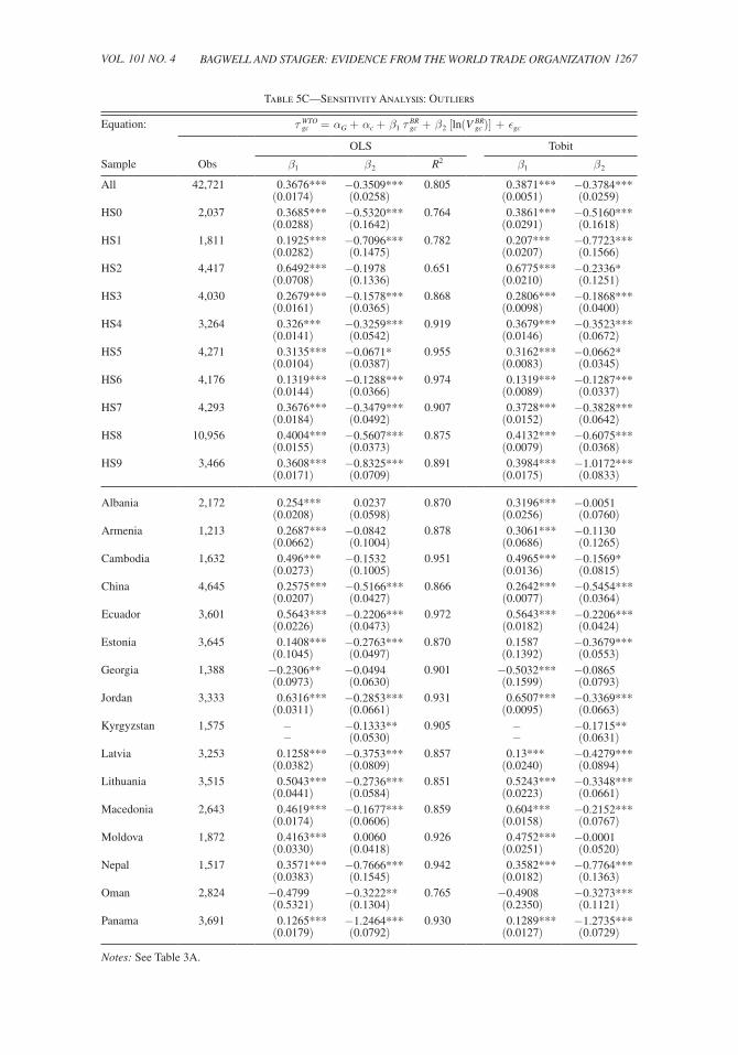
1267BAgWELL And sTAigER: EvidEncE fROm ThE WORLd TRAdE ORgAnizATiOnvOL. 101 nO. 4
Table 5C—Sensitivity Analysis: Outliers
Equation: τ gc WTO = α g + α c + β 1 τ gc
BR + β 2 [ln( v gc BR )] + ϵ gc
OLS Tobit
Sample Obs β 1 β 2 R2 β 1 β 2
All 42,721 0.3676*** −0.3509*** 0.805 0.3871*** −0.3784***(0.0174) (0.0258) (0.0051) (0.0259)
HS0 2,037 0.3685*** −0.5320*** 0.764 0.3861*** −0.5160***(0.0288) (0.1642) (0.0291) (0.1618)
HS1 1,811 0.1925*** −0.7096*** 0.782 0.207*** −0.7723***(0.0282) (0.1475) (0.0207) (0.1566)
HS2 4,417 0.6492*** −0.1978 0.651 0.6775*** −0.2336*(0.0708) (0.1336) (0.0210) (0.1251)
HS3 4,030 0.2679*** −0.1578*** 0.868 0.2806*** −0.1868***(0.0161) (0.0365) (0.0098) (0.0400)
HS4 3,264 0.326*** −0.3259*** 0.919 0.3679*** −0.3523***(0.0141) (0.0542) (0.0146) (0.0672)
HS5 4,271 0.3135*** −0.0671* 0.955 0.3162*** −0.0662*(0.0104) (0.0387) (0.0083) (0.0345)
HS6 4,176 0.1319*** −0.1288*** 0.974 0.1319*** −0.1287***(0.0144) (0.0366) (0.0089) (0.0337)
HS7 4,293 0.3676*** −0.3479*** 0.907 0.3728*** −0.3828***(0.0184) (0.0492) (0.0152) (0.0642)
HS8 10,956 0.4004*** −0.5607*** 0.875 0.4132*** −0.6075***(0.0155) (0.0373) (0.0079) (0.0368)
HS9 3,466 0.3608*** −0.8325*** 0.891 0.3984*** −1.0172***(0.0171) (0.0709) (0.0175) (0.0833)
Albania 2,172 0.254*** 0.0237 0.870 0.3196*** −0.0051(0.0208) (0.0598) (0.0256) (0.0760)
Armenia 1,213 0.2687*** −0.0842 0.878 0.3061*** −0.1130(0.0662) (0.1004) (0.0686) (0.1265)
Cambodia 1,632 0.496*** −0.1532 0.951 0.4965*** −0.1569*(0.0273) (0.1005) (0.0136) (0.0815)
China 4,645 0.2575*** −0.5166*** 0.866 0.2642*** −0.5454***(0.0207) (0.0427) (0.0077) (0.0364)
Ecuador 3,601 0.5643*** −0.2206*** 0.972 0.5643*** −0.2206***(0.0226) (0.0473) (0.0182) (0.0424)
Estonia 3,645 0.1408*** −0.2763*** 0.870 0.1587 −0.3679***(0.1045) (0.0497) (0.1392) (0.0553)
Georgia 1,388 −0.2306** −0.0494 0.901 −0.5032*** −0.0865(0.0973) (0.0630) (0.1599) (0.0793)
Jordan 3,333 0.6316*** −0.2853*** 0.931 0.6507*** −0.3369***(0.0311) (0.0661) (0.0095) (0.0663)
Kyrgyzstan 1,575 − −0.1333** 0.905 − −0.1715**− (0.0530) − (0.0631)
Latvia 3,253 0.1258*** −0.3753*** 0.857 0.13*** −0.4279***(0.0382) (0.0809) (0.0240) (0.0894)
Lithuania 3,515 0.5043*** −0.2736*** 0.851 0.5243*** −0.3348***(0.0441) (0.0584) (0.0223) (0.0661)
Macedonia 2,643 0.4619*** −0.1677*** 0.859 0.604*** −0.2152***(0.0174) (0.0606) (0.0158) (0.0767)
Moldova 1,872 0.4163*** 0.0060 0.926 0.4752*** −0.0001(0.0330) (0.0418) (0.0251) (0.0520)
Nepal 1,517 0.3571*** −0.7666*** 0.942 0.3582*** −0.7764***(0.0383) (0.1545) (0.0182) (0.1363)
Oman 2,824 −0.4799 −0.3222** 0.765 −0.4908 −0.3273***(0.5321) (0.1304) (0.2350) (0.1121)
Panama 3,691 0.1265*** −1.2464*** 0.930 0.1289*** −1.2735***(0.0179) (0.0792) (0.0127) (0.0729)
notes: See Table 3A.

1268 ThE AmERicAn EcOnOmic REviEW JunE 2011
Finally, we present the results of estimating the more general specification in (14b) on a five-country subsample (China, Ecuador, Latvia, Lithuania, and Oman) using the Broda, Limão, and Weinstein (2008) import demand and foreign export supply elasticities. This provides an important opportunity to check within this sub-sample that our main results are not driven by the linearity restrictions that underlie (14a). We also use these elasticities to allow for the possibility of free-riding in WTO negotiations, and report results that explore the robustness of our results to the possibility of free-riding within the context of WTO accession negotiations.
We estimate (14b) in semi-log form (following the approach preferred by Broda, Limão, and Weinstein (2008) to dealing with outliers in the inverse elasticity mea-sure) according to
τ gc WTO = α g + α c + ϕ 1 τ gc BR + ϕ 2 [ln( η gc BR )] + υ gc ,
where recall that η BR ≡ [( σ BR / ω *BR ) ( m BR / p BR )] is the general international cost-shifting term central to the terms-of-trade theory. The measures of σ BR and ω *BR are available at the four-digit HS level for each of the five countries in our sub-sample, and so we assume when constructing the variable η BR that these elasticities are the same for all six-digit HS products within a four-digit HS industry. To address possible measurement error issues associated with σ BR and ω *BR , we follow Broda, Limão, and Weinstein and construct for each country c an instrument for ln( η gc BR ) using the average elasticity measures for all countries but c in their sample, and we present instrumental variables (IV) estimates of ϕ 1 and ϕ 2 .33 According to the terms-of-trade theory, the estimated ϕ 1 should be positive while the estimated ϕ 2 should be negative.
The first column of Table 6 presents the IV estimates for the full (sub) sample, by sector, and by country.34 As can be seen, the broad level of support for the terms-of-trade theory reflected in our earlier results is robust to this generalization. In fact, comparing the estimates in the first column of Table 6 to the estimates in Table 3A which are based on (14a), the pattern of significance across sectors and countries is unchanged. This suggests that our main results are not driven by the linearity restric-tions that underlie (14a). Moreover, it is difficult to think of alternatives to the terms-of-trade theory that would suggest a negative relationship between τ gc WTO and η gc BR , and so the supportive findings based on (14b) make it less likely as well that our main results based on the simpler relationship in (14a) reflect spurious correlations.35
33 A complete description of each instrument used in the paper is contained in the online Data Appendix.34 We note that the first-stage estimates perform well. For example, the first-stage f-statistic for the pooled
sample is 288.9. Also, following Brent R. Moulton (1990), it is increasingly common to provide “cluster-adjusted” standard errors when employing “mixed-level” data that do not all vary at the same level of aggregation (although, see Charles F. Wellford, John Pepper, and Carol V. Petrie (2003) for a detailed discussion of the pros and cons of cluster-adjusted standard errors). All of our regressors vary at the six-digit level along with the dependent variable, but because some of the regressors employed in Table 6 (e.g., ln( η gc BR )) are constructed with the measures of σ BR and/or ω *BR that vary at the four-digit level, it might be argued that cluster-adjusted standard errors are appropri-ate for those results. While we do not report cluster-adjusted standard errors, the broad findings we emphasize in Table 6 hold also when significance is judged by cluster-adjusted standard errors (clustered by HS four-digit indus-tries or by country and HS four-digit industries), although with some loss of significance as would be expected.
35 As a check for endogeneity, we also tried instrumenting τ gc BR and ln( η gc BR ) with the average τ gc BR and ln( η gc BR ) for the remaining countries in our sample. Relative to the results we report in Table 6, the pooled results under this alternative estimation are unchanged, the by-sector results are slightly weaker and the by-country results are slightly stronger, but overall the support for the terms-of-trade theory is comparable.

1269BAgWELL And sTAigER: EvidEncE fROm ThE WORLd TRAdE ORgAnizATiOnvOL. 101 nO. 4
The elasticity measures reported in Broda, Limão, and Weinstein (2008) also allow us to consider for this five-country subsample the possibility of MFN free-riders. When the decision to participate in tariff negotiations is made on a good-by-good basis, Ludema and Mayda (2007) argue that the MFN free-riding problem arises when foreign exporter concentration (as measured by the Herfindahl index) is low and the importing country’s ability to affect world prices with its tariff choices is high; and they report evidence of a negative relationship between bound tariff rates and an interaction term between the Herfindahl index of foreign exporter con-centration and measures of importer market power. In the context of the accession negotiations that are our concern here, the participation decision is in practice made on a bilateral country-by-country basis rather than good by good (see, for example, WTO 2005, pp. 12–30), and so it is not clear that the free-rider logic described by
Table 6—Nonlinear Specifications
τ gc WTO = α g + α c + ϕ 1 τ gc
BR + ϕ 2 [ln( η gc BR )] + υ gc τ gc WTO = α g + α c + ϕ 1 τ gc
BR + ϕ 2 [ln( η gc BR )] + ϕ 3 [ Θ gc BR ] + υ gc
IV-GMM IV-GMM
Sample Obs ϕ 1 ϕ 2 Obs ϕ 1 ϕ 2 ϕ 3
All 15,645 0.1984*** −0.4154*** 15,645 0.1857*** −0.4671*** −2.2979***(0.0205) (0.0515) (0.0216) (0.0662) (0.6519)
HS0 789 0.0153 −1.8375*** 789 −1.1907 −0.9786 −112.8735(0.0832) (0.4212) (5.9855) (4.7322) (520.5452)
HS1 607 0.0671** −1.6040*** 607 0.0758** −1.4991*** 0.7296(0.0296) (0.4771) (0.0362) (0.4315) (2.8101)
HS2 1,734 0.0237 −0.4269* 1,734 0.0266 −0.4144* 0.7462(0.0937) (0.2358) (0.0960) (0.2328) (2.5375)
HS3 1,516 0.3399*** −0.1342*** 1,516 0.3684*** −0.0717 −1.1613*(0.0373) (0.0482) (0.0422) (0.0588) (0.6528)
HS4 1,193 0.3494*** −0.2099** 1,193 0.4345*** −0.0626 −3.1277(0.0298) (0.0935) (0.1172) (0.1846) (4.6537)
HS5 1,534 0.2956*** −0.4381*** 1,534 0.2632*** −0.0680 0.9875**(0.0135) (0.1150) (0.0186) (0.0821) (0.3683)
HS6 1,550 0.1941*** −0.1404*** 1,550 0.1964*** −0.1385** −0.1556(0.0219) (0.0512) (0.0223) (0.0495) (0.2998)
HS7 1,449 0.4929*** −0.2027** 1,449 0.4820*** −0.2789*** 1.7452(0.0353) (0.0812) (0.0364) (0.0841) (1.1590)
HS8 4,108 0.3291*** −0.3387*** 4,108 0.3277*** −0.3382*** −0.1092(0.0293) (0.0511) (0.0297) (0.0509) (0.2329)
HS9 1,165 0.3589*** 0.0674 1,165 0.3898*** 0.3157* 2.7177***(0.0488) (0.1243) (0.0584) (0.1753) (0.6446)
China 4,371 0.2148*** −0.5384*** 4,371 0.2145*** −0.5381*** −0.0284(0.0216) (0.0499) (0.0225) (0.0480) (0.4689)
Ecuador 3,108 0.5236*** −0.3149*** 3,108 0.5416*** −0.4041*** −1.2416*(0.0242) (0.0685) (0.0308) (0.1222) (0.6728)
Latvia 2,983 0.1022** −0.2994** 2,983 0.0907** −0.2349 2.6329(0.0416) (0.1200) (0.0444) (0.1629) (1.8390)
Lithuania 3,088 0.4355*** −0.1625* 3,088 0.4420*** −0.1514* −0.2955(0.0464) (0.0941) (0.0485) (0.0899) (0.5021)
Oman 2,095 −0.7157 −0.4886*** 2,095 −1.2108* −0.5428** −5.5640(0.6267) (0.1728) (0.7000) (0.2476) (3.5050)
notes: See Table 3A.

1270 ThE AmERicAn EcOnOmic REviEW JunE 2011
Ludema and Mayda applies. But it is important to check that our main results are robust to the possibility of an MFN free-rider problem.
To this end, with m gck BR denoting country c’s pre-negotiation quantity of imports
of product g from foreign exporting country k, and letting WTO denote the set of WTO-member countries, we define the Herfindahl index of foreign exporter concentration by gc BR ≡ ∑ k∈WTO
( m gck BR ) 2 / ( ∑ k∈WTO
m gck BR ) 2 .36 We then define Θ gc BR
≡ gc BR ⋅ ln(1/ ω *BR ) (assuming, as before, that ω *BR is the same for all six-digit HS products within a four-digit HS industry) and estimate
τ gc WTO = α g + α c + ϕ 1 τ gc BR + ϕ 2 [ln( η gc BR )] + ϕ 3 [ Θ gc BR ] + υ gc ,
instrumenting for both ln( η gc BR ) and Θ gc BR along the lines described above. According to the terms-of-trade theory, the estimated ϕ 1 should be positive and ϕ 2 negative, while the estimated ϕ 3 should be negative if a significant MFN free-rider problem is present.
The results of the IV estimation on the full (sub) sample, by sector and by country, are contained in the second column of Table 6. As can be seen, the results continue to show broad support for the terms-of-trade theory: the full-sample estimates of ϕ 1 and ϕ 2 are of the expected sign and highly significant, and the by-country estimates show a level of support for the theory that is roughly in line with the results for these countries presented in earlier tables; the by-sector estimates of ϕ 2 lose some of their significance compared to earlier results, but are still broadly supportive of the theory as well. Turning to the estimate of ϕ 3 , which should be negative if a significant MFN free-rider problem is present, our results paint a more qualified picture. The full-sample estimate of ϕ 3 is significantly negative, suggesting that the free-rider issue may be a problem in WTO accession negotiations. On the other hand, none of the by-country estimates of ϕ 3 are significantly different from zero, while none of the by-sector estimates of ϕ 3 are significantly negative (and two are significantly positive). Taken together, the evidence in the second column of Table 6 suggests that some free-rider issues may be present in the context of WTO accession negotiations, but that these issues are not likely to be a major factor in determining the tariff cuts agreed to by acceding countries. As we have observed, this finding seems consistent with the nature of the accession negotiations on which we focus.
V. Conclusion
What do trade negotiators negotiate about? According to the terms-of-trade theory, they negotiate to build an avenue of escape from a terms-of-trade-driven prisoner’s dilemma. In this paper we use the terms-of-trade theory to develop a relationship that predicts negotiated tariff levels on the basis of pre-negotiation data: tariffs, import vol-umes and prices, and trade elasticities. And we show for linear demands and supplies that this relationship takes a particularly simple form: the magnitude of the negotiated tariff cut predicted by the terms-of-trade theory rises proportionately with the ratio of pre-negotiation import volume to world price. We confront these predicted relation-
36 In instances when ∑ k∈WTO m gck BR
= 0, which is the case for roughly 6 percent of the observations in our sample, we define gc BR ≡ 0. Our definition of the Herfindahl index is slightly different from that adopted by Ludema and Mayda (2007, 2009), because they treat non-GATT/WTO members slightly differently than we do.
1271BAgWELL And sTAigER: EvidEncE fROm ThE WORLd TRAdE ORgAnizATiOnvOL. 101 nO. 4
ships with data on the outcomes of tariff negotiations associated with the accession of new WTO members. We find strong and robust support for the central predictions of the terms-of-trade theory in the observed pattern of negotiated tariff cuts.
Our paper provides the first empirical assessment of the central predictions of the terms-of-trade theory of trade agreements. The results are promising for the theory, but they also reflect some important limitations. For one, we have limited our analysis to the consideration of MFN tariff bargaining. But the vast majority of WTO members have also granted discriminatory preferential tariff access to a sub-set of their trading partners through free trade agreements, customs unions, and the generalized system of preferences. For another, we have abstracted from the possi-bility that enforcement difficulties might prevent WTO negotiations from achieving points on the international efficiency frontier, assuming instead that the discrepancy between WTO negotiating outcomes and free trade can be attributed entirely to the underlying political economy forces of each member government. But there are many reasons to expect that limited enforcement ability could place binding con-straints on achievable negotiating outcomes in the WTO. Exploring ways to incor-porate each of these features into the empirical analysis of WTO tariff bargaining could lead to important new insights.
Moreover, we have limited our empirical work to a focus on new members of the WTO that joined after its creation at the end of the Uruguay Round of GATT negotiations, in order to identify a set of countries that arguably traversed from their tariff reaction curves to the efficiency frontier in one negotiating round. But it is important to find ways to extend the empirical analysis of WTO tariff bargaining to the entire set of (currently) 153 member governments. It might be argued that many of the developing country members who were also GATT members and/or who joined the WTO at its inception accepted their first meaningful tariff bindings in the Uruguay Round, and so our approach might be extended to include these countries in a straightforward manner. Given that more than two-thirds of WTO members are developing countries, such an extension could significantly broaden country cover-age. Finding a way to incorporate the industrial country members into the empirical analysis of WTO tariff bargaining is more difficult in light of the many rounds of negotiation in which they have actively participated, but this is perhaps even more important for the theory.
In light of these and other important limitations of our study, we can claim only to have offered a first, albeit promising, glimpse at the central empirical content of the terms-of-trade theory. Providing more conclusive evidence is an important task for future research.
REFERENCES
Anderson, James E., and Eric van Wincoop. 2002. “Borders, Trade, and Welfare.” In Brookings Trade forum 2001, ed. Dani Rodrik and Susan Collins, 207–43. Washington, DC: Brookings Institution Press.
Bagwell, Kyle. 2009. “Self-Enforcing Trade Agreements and Private Information.” National Bureau of Economic Research Working Paper 14812.
Bagwell, Kyle, and Robert W. Staiger. 1999. “An Economic Theory of GATT.” American Economic Review, 89(1): 215–48.
Bagwell, Kyle, and Robert W. Staiger. 2001. “Reciprocity, Non-Discrimination and Preferential Agree-ments in the Multilateral Trading System.” European Journal of Political Economy, 17(2): 281–325.

1272 ThE AmERicAn EcOnOmic REviEW JunE 2011
Bagwell, Kyle, and Robert W. Staiger. 2002. The Economics of the World Trading system. Cambridge,MA: MIT Press.
Bagwell, Kyle, and Robert W. Staiger. 2005. “Enforcement, Private Political Pressure, and the General Agreement on Tariffs and Trade/World Trade Organization Escape Clause.” Journal of Legal stud-ies, 34(2): 471–513.
Bagwell, Kyle, and Robert W. Staiger. 2006. “What Do Trade Negotiators Negotiate About? Empiri-cal Evidence from the World Trade Organization.” National Bureau of Economic Research Work-ing Paper 12727.
Bagwell, Kyle, and Robert W. Staiger. 2011. “What Do Trade Negotiators Negotiate About? Empirical Evidence from the World Trade Organization: Dataset.” American Economic Review. http://www.aeaweb.org/articles.php?doi=10.1257/aer.101.4.1238.
Bown, Chad P. 2002. “The Economics of Trade Disputes, the GATT’s Article XXIII, and the WTO’s Dispute Settlement Understanding.” Economics and Politics, 14(3): 283–323.
Bown, Chad P. 2004a. “Trade Disputes and the Implementation of Protection under the GATT: An Empirical Assessment.” Journal of international Economics, 62(2): 263–94.
Bown, Chad P. 2004b. “On the Economic Success of GATT/WTO Dispute Settlement.” Review of Eco-nomics and statistics, 86(3): 811–23.
Bown, Chad P. 2004c. “Trade Policy under the GATT/WTO: Empirical Evidence of the Equal Treat-ment Rule.” canadian Journal of Economics, 37(3): 678–720.
Bown, Chad P., and Meredith A. Crowley. 2006. “Policy Externalities: How U.S. Antidumping Affects Japanese Exports to the EU.” European Journal of Political Economy, 22(3): 696–714.
Broda, Christian, Nuno Limão, and David E. Weinstein. 2008. “Optimal Tariffs and Market Power: The Evidence.” American Economic Review, 98(5): 2032–65.
Chang, Won, and L. Alan Winters. 2002. “How Regional Blocs Affect Excluded Countries: The Price Effects of Mercosur.” American Economic Review, 92(4): 889–904.
Estevadeordal, Antoni, Caroline Freund, and Emanuel Ornelas. 2008. “Does Regionalism Affect Trade Liberalization toward Nonmembers?” Quarterly Journal of Economics, 123(4): 1531–75.
Evenett, Simon J., Jonathan Gage, and Maxine Kennett. 2004. “WTO Membership and Market Access: Evidence from the Accessions of Bulgaria and Ecuador.” Unpublished.
Hoekman, Bernard, and Michel Kostecki. 2001. The Political Economy of the World Trading system: from gATT to WTO. Oxford: Oxford University Press.
Horn, Henrik, Giovanni Maggi, and Robert W. Staiger. “Trade Agreements as Endogenously Incomplete Contracts.” American Economic Review, 100(1): 394–419.
Johnson, Harry G. 1953. “Optimum Tariffs and Retaliation.” Review of Economic studies, 21(2): 142–53.Karacaovali, Baybars, and Nuno Limão. 2008. “The Clash of Liberalizations: Preferential versus Mul-
tilateral Trade Liberalization in the European Union.” Journal of international Economics, 74(2): 299–327.
Kee, Hiau Looi, Alessandro Nicita, and Marcelo Olarreaga. 2009. “Estimating Trade Restrictiveness Indices.” Economic Journal, 119(534): 172–99.
Kee, Hiau Looi, Alessandro Nicita, and Marcelo Olarreaga. 2009. “Estimating Trade Restrictiveness Indices Dataset.” http://go.worldbank.org/C5VQJIV3H0.
Kreinin, Mordechai. 1961. “Effect of Tariff Changes on the Prices and Volumes of Imports.” American Economic Review, 51(3):310–24.
Krugman, Paul. 1997. “What Should Trade Negotiators Negotiate About?” Journal of Economic Lit-erature, 35(1): 113–20.
Limão, Nuno. 2006. “Preferential Trade Agreements as Stumbling Blocks for Multilateral Trade Liber-alization: Evidence for the United States.” American Economic Review, 96(3): 896–914.
Ludema, Rodney D., and Anna Maria Mayda. 2007. “The Free-riding Effect of the MFN Clause: Evi-dence across Countries.” Unpublished.
Ludema, Rodney D., and Anna Maria Mayda. 2009. “Do Countries Free Ride on MFN?” Journal of international Economics, 77(2): 137–50.
Maggi, Giovanni, and Andres Rodriguez-Clare. 2007. “A Political-Economy Theory of Trade Agree-ments.” American Economic Review, 97(4): 1374–406.
Mayer, Wolfgang. 1981. “Theoretical Considerations on Negotiated Tariff Adjustments.” Oxford Eco-nomic Papers, 33(1): 135–53.
Moulton, Brent R. 1990. “An Illustration of a Pitfall in Estimating the Effects of Aggregate Variables on Micro Unit.” Review of Economics and statistics, 72(2): 334–38.
Rigobon, Roberto, and Thomas M. Stoker. 2007. “Estimation with Censored Regressors: Basic Issues.” international Economic Review, 48(4): 1441–67.
Rose, Andrew K. 2004a. “Do We Really Know That the WTO Increases Trade?” American Economic Review, 94(1): 98–114.
1273BAgWELL And sTAigER: EvidEncE fROm ThE WORLd TRAdE ORgAnizATiOnvOL. 101 nO. 4
Rose, Andrew K. 2004b. “Do WTO Members Have More Liberal Trade Policy?” Journal of interna-tional Economics, 63(2): 209–35.
Rose, Andrew K. 2004c. “Does the WTO Make Trade More Stable?” National Bureau of Economic Research Working Paper 10207.
Soloaga, Isidro, Marcelo Olarreaga, and Alan Winters. 1999. “What’s Behind Mercosur’s Common External Tariff?” The World Bank, Policy Research Working Paper 2231.
Subramanian, Arvind, and Shang-Jin Wei. 2007. “The WTO Promotes Trade, Strongly but Unevenly.” Journal of international Economics, 72(1): 151–75.
Tomz, Michael, Judith L. Goldstein, and Douglas Rivers. 2007. “Do We Really Know That the WTO Increases Trade? Comment.” American Economic Review, 97(5): 2005–18.
Wellford, Charles F., John Pepper, and Carol V. Petrie. 2003. Firearms and Violence: A Critical Review. National Research Council, Committee on Law and Justice and Committee on National Statistics, Division of Behavioral and Social Sciences and Education. Washington, D.C.
Winters, L. Alan, and Won Chang. 2000. “Regional Integration and Import Prices: An Empirical Inves-tigation.” Journal of international Economics, 51(2): 363–77.
WTO. 2005. “Technical Note on the Accession Process—Note by the Secretariat—Revision.” Novem-ber 28, WT/ACC/10/Rev.3, Geneva.
WTO. 2007. “World Trade Report 2007.” The World Trade Organization, Geneva.WTO. 2008. “World Tariff Profiles 2008.” The World Trade Organization, Geneva.Yongtu, Long. 2000. Statement Given at the Tenth Session of the Working Party on China, World Trade
Organization, Geneva, June 23.
This article has been cited by:
1. Kyle Bagwell, , Robert W. Staiger. 2011. What Do Trade Negotiators Negotiate About? EmpiricalEvidence from the World Trade OrganizationWhat Do Trade Negotiators Negotiate About?Empirical Evidence from the World Trade Organization. American Economic Review 101:4,1238-1273. [Abstract] [View PDF article] [PDF with links]