What Are Uncertainty Shocks?∗

Nicholas Kozeniauskas, Anna Orlik and Laura Veldkamp†

June 13, 2018

Abstract

Many modern business cycle models use uncertainty shocks to generate aggregate fluc-tuations. However, uncertainty is measured in a variety of ways. Our analysis shows thatthe measures are not the same, either statistically or conceptually, raising the question ofwhether fluctuations in them are actually generated by the same phenomenon. We propose amechanism that generates realistic micro dispersion (cross-sectional variance of firm-level out-comes), higher-order uncertainty (disagreement) and macro uncertainty (uncertainty aboutmacro outcomes) from changes in macro volatility. If we want to consider “uncertaintyshocks” as a unified phenomenon, these results show what such a shock might actually en-tail.

JEL codes: E32, E37

1 Introduction

One of the primary innovations in modern business cycle research is the idea that uncertainty

shocks drive aggregate fluctuations. A recent literature starting with Bloom (2009) demonstrates

that uncertainty shocks can explain business cycles, financial crises and asset price fluctuations

with great success (e.g., Bloom et al., 2018; Ordonez, 2013; Pastor and Veronesi, 2012). But the

measures of uncertainty are wide-ranging. Changes in the volatility of stock prices (VIX), dis-

agreement among macro forecasters, and the cross-sectional dispersion in firms’ earnings growth,

while all used as measures of uncertainty, are not the same. Comparing VIX and firm earnings

growth dispersion is like comparing business cycle volatility and income growth inequality. One

measures aggregate changes in the time-series and the other differences in a cross-section. Are

∗We are grateful to Ricardo Reis and an anonymous referee for their insightful comments, and to VirgiliuMidrigan, Simon Mongey, and Tom Sargent for useful discussions and suggestions. The feedback from participantsat the SED meetings in Warsaw and the AEA meetings in San Francisco is also greatly appreciated.†Affiliations: Banco de Portugal (Nicholas Kozeniauskas); Board of Governors of the Federal Reserve System

(Anna Orlik); Columbia University, Graduate School of Business, Department of Finance (Laura Veldkamp). Forcorrespondence please email Nicholas Kozeniauskas at nic.j.koz@nyu.edu.

1

these disparate measures really capturing a common underlying shock? If so, what is it? Un-

certainty is not exogenous. People do not spontaneously become uncertain, for no good reason.

One person might. But a whole economy changing its beliefs, unprompted, is collective mania.

Instead, people become uncertain after observing an event that makes them question future out-

comes. That raises the question: What sorts of events can make agents uncertain in a way that

shows up in all these disparate measures? Uncovering the answer to this question opens the door

to understanding what this uncertainty shock is and why the aggregate economy fluctuates.

This paper contributes to answering these questions in the following ways. First it shows that

the various measures of uncertainty are statistically distinct. While most measures of uncertainty

are positively correlated after controlling for the business cycle, even the most correlated measures

have correlations that are far from unity and some measures have correlations close to zero. Thus

it is not obvious that these various measures of uncertainty are measuring the same shock to

the economy. Using a model we show that, depending on the type of shock, different types of

uncertainty can covary positively or negatively. The fact that these distinct measures are conflated

in the literature is troubling because it means that there is not one uncertainty shock that explains

the various aggregate outcomes linked to uncertainty. The discovery of many different shocks that

explain many different outcomes is not the unified theory of fluctuations one would hope for.

To unify uncertainty measures a model is used to identify a type of shock that can generate

comovement in the different types of uncertainty that is consistent with the data. The model

shows that changes in macroeconomic volatility are a quantitatively plausible explanation.

Section 2 starts with a statistical exploration of various uncertainty measures. These mea-

sures are organized into three categories: measures of uncertainty about macroeconomic outcomes

(macro uncertainty); measures of the dispersion of firm outcomes (micro dispersion); and mea-

sures of the uncertainty that people have about what others believe (higher-order uncertainty).

The first result is that some measures are statistically unrelated to others, except for the fact that

all are countercyclical. However, the data offers some hope for resuscitating uncertainty shocks

as a unified phenomenon. Statistically there is a rationale for the practice of assigning a common

name to some of these time-series, cross-sectional, output, price and forecast measures: A set of

measures of these three types of uncertainty and dispersion have some common fluctuations at

their core. This is not just a business cycle effect. These measures comove significantly above and

beyond what the cycle alone can explain.

2

To understand these correlations and attempt to identify what kind of shock could generate

them, a model is used (Section 3). In the model agents observe events, receive some private

information, update beliefs with Bayes’ law, form expectations and choose economic inputs in

production. In this framework the three types of uncertainty and dispersion are formally defined

and solved for. The model has three possible second moment shocks that could generate fluctu-

ations in uncertainty: changes in public signal noise, changes in private signal noise and changes

in macro volatility. An increase in signal noise represents the idea that some information sources,

such as news, ratings, or insights from a person’s contacts might be less reliable or more open to

interpretation.

Section 4 investigates the implications of the three possible shocks to the economy for the

covariance of the three types of uncertainty and dispersion. The analysis shows that it is not given

that the three types of uncertainty and dispersion are positively correlated. Their correlations

can be negative. This shows that the different types of uncertainty are theoretically distinct.

Therefore if we want to think of the various uncertainty shocks as a unified phenomenon, then

there needs to be a common origin for them. The negative correlations can arise when there are

shocks to signal noise. For example, when signals are noisier, they convey less information, leaving

agents with more macro uncertainty. At the same time, noisier signals get less weight in agents’

beliefs. Since differences in signals are the source of agents’ disagreement, weighting them less

reduces disagreement, which results in less dispersed firm decisions (lower micro dispersion) and

less dispersed forecasts (lower higher-order uncertainty).

In contrast, macro volatility fluctuations are a reliable common cause of the disparate collec-

tion of changes referred to as uncertainty shocks. Macro volatility creates macro uncertainty by

making prior macro outcomes less accurate predictors of future outcomes. They create dispersion

because when agents’ prior information is less accurate, they weight that prior information less

and weight signals more. This change in signal weighting generates greater differences in beliefs.

Prior realizations are public information: Everyone saw the same GDP yesterday. But signals are

heterogeneous. While one firm may incorporate their firm’s sales numbers, another will examine

its competitors’ prices, and yet another will purchase a forecast from one of many providers. When

macro uncertainty rises and prior realizations are weighted less, these heterogeneous sources of

information are weighted more, driving beliefs apart.

Divergent beliefs (forecasts) create higher-order uncertainty and micro dispersion. When fore-

3

casts differ, and the difference is based on information others did not observe, another person’s

forecast becomes harder to predict. This is higher-order uncertainty. Firms with divergent fore-

casts also choose different inputs and obtain different outputs. This is more micro dispersion.

All three forms of uncertainty and their covariance can be explained in a unified framework that

brings us one step closer to understanding what causes business cycle fluctuations.

While our model points to plausible sources of uncertainty measure comovement, it misses a

mechanism to make uncertainty countercyclical. Of course one could assume that macro volatility

rises in recessions, as many theories do. But since our goal is to uncover sources of fluctuations,

it makes sense to ask why. To explain why uncertainty is countercyclical, the model needs one

additional ingredient: disaster risk. Disaster risk is incorpoarted by allowing the TFP growth

process to have non-normal innovations. Normal distributions have thin tails, which makes disas-

ters incredibly unlikely, and are symmetric so that disasters and miracles are equally likely. This

is not what the data looks like. GDP growth is negatively skewed and our extension allows the

model to have this feature. Disaster risk is important for understanding uncertainty because dis-

aster probabilities are difficult to assess, so a rise in disaster risk creates both uncertainty about

aggregate outcomes (macro uncertainty) and disagreement; and this is especially so in recessions

when disasters are more likely.

Section 5 explores whether our model is quantitatively plausible. The simple model presented

in Section 3 generates half of the fluctuations and most of the correlations of the various un-

certainty measures. Adding disaster risk makes these uncertainty measures countercyclical. It

also amplifies uncertainty fluctuations. The reason is that disasters are rare and difficult to pre-

dict. When outcomes are difficult to predict, firms disagree (higher-order uncertainty); they make

different input choices and have heterogeneous outcomes (micro dispersion). With the learning

and disaster risk mechanisms operating together, the model is able to generate over two thirds

of the fluctuations in the various uncertainty measures. The uncertainty measures also comove

appropriately with the business cycle and each other.

Related literature In his seminal paper, Bloom (2009) showed that various measures of uncer-

tainty are countercyclical and studied the ability of uncertainty shocks to explain business cycle

fluctuations. Since then, many other papers have further investigated uncertainty shocks as a

4

driving force for business cycles.1 A related strand of literature studies the impact of uncertainty

shocks on asset prices.2 Our paper complements this literature by investigating the nature and

origins of their exogenous uncertainty shocks.

A few recent papers also question the origins of uncertainty shocks. Some propose reasons

for macro uncertainty to fluctuate.3 Others explain why micro dispersion is countercyclical.4

Ludvigson et al. (2018) use statistical projection methods to argue that output fluctuations can

cause uncertainty fluctuations or the other way around, depending on the type of uncertainty.

Our paper differs because it explains not just statistically, but also economically, why dispersion

across firms and forecasters is connected to uncertainty about aggregate outcomes, beyond what

the business cycle can explain.

Finally, the tail risk mechanism that amplifies uncertainty changes in our quantitative exercise

(Section 5) is also used in Orlik and Veldkamp (2015) to explain why macro uncertainty fluctu-

ates and in Kozlowski et al. (2017) to explain business cycle persistence. This paper takes such

macro changes as given and uses tail risk to amplify micro dispersion and higher-order uncertainty

covariance. The models in these other papers do not have heterogeneity in beliefs, and therefore

cannot possibly address the central question of this paper: the distinction and connections between

aggregate outcome uncertainty, micro dispersion and belief heterogeneity.

2 Uncertainty Measures and Uncertainty Facts

This section makes two points. First, different types of uncertainty are statistically distinct—they

have correlations that are far less than one—which raises the question of whether they should be

treated as the same phenomenon. Second, some measures have a significant positive relationship

above and beyond the business cycle, which suggests that there is a force that links them. This

section starts with measurement and definitions. We discuss three types of uncertainty that have

1e.g., Bloom et al. (2018), Basu and Bundick (2017), Bianchi et al. (2018), Arellano et al. (2018), Christianoet al. (2014), Gilchrist et al. (2014), Schaal (2017). Bachmann and Bayer (2013) dispute the effect of uncertaintyon aggregate activity.

2e.g., Bansal and Shaliastovich (2010) and Pastor and Veronesi (2012).3In Nimark (2014), the publication of a signal conveys that the true event is far away from the mean, which

increases macro uncertainty. Benhabib et al. (2016) consider endogenous information acquisition. In Van Nieuwer-burgh and Veldkamp (2006) and Fajgelbaum et al. (2017) less economic activity generates less data, which increasesuncertainty.

4Bachmann and Moscarini (2012) argue that price dispersion rises in recessions because it is less costly for firmsto experiment with their prices then. Decker et al. (2016) argue that firms have more volatile outcomes in recessionsbecause they can access fewer markets and so diversify less.

5

been used in the literature and introduce various measures of them. While it is well known that

these measures are countercyclical, less is know about the relationship between the different types

of uncertainty, which is our focus.

Conceptually there are three types of uncertainty that have been used in existing research.

In some papers an uncertainty shock means that an aggregate variable, such as GDP, becomes

less predictable.5 This will be referred to as macro uncertainty. In other papers an uncertainty

shock describes an increase in the uncertainty that firms have about their own outcomes due to

changes in idiosyncratic variables. This is micro uncertainty.6 Higher-order uncertainty describes

the uncertainty that people have about others’ beliefs, which usually arises when forecasts differ.7

To measure macro uncertainty, it would be ideal to know the variance (or confidence bounds)

of peoples’ beliefs about future macro outcomes. A common proxy for this is the VIX, which is

a measure of the future volatility of the stock market, implied by options prices. To the extent

that macro outcomes are reflected in stock prices and the assumptions underlying options pricing

formulas are correct, this is a measure of the unpredictability of future aggregate outcomes, or

macro uncertainty. Bloom (2009) constructs a series for macro uncertainty based on this and

extends it back in time using the actual volatility of stock prices for earlier periods in which the

VIX is not available. This series will be referred to as VIX. Full details of this measure and all of

the uncertainty measures used in this paper are provided in the online appendix.8 A second proxy

for macro uncertainty is the average absolute error of GDP growth forecasts, labelled forecast

errors from here on. Assuming more uncertainty is associated with more volatile future outcomes,

forecast errors will be higher on average when uncertainty is higher. This measure is constructed

using data on real GDP growth forecasts from the Survey of Professional Forecasters (SPF). The

third measure of macro uncertainty comes from Jurado et al. (2015) and will be called the JLN

uncertainty series in reference to those authors’ names. Their measure of macro uncertainty is an

econometric measure based on the variance of forecasts of macro variables made using a very rich

dataset.

True micro uncertainty is difficult to measure because data on firms’ beliefs is rare. Dispersion

5For macro uncertainty shocks see, for example, Basu and Bundick (2017) and Bianchi et al. (2018) on businesscycles, and Bansal and Shaliastovich (2010) and Pastor and Veronesi (2012) in the asset pricing literature.

6For micro uncertainty shocks see, for example, Arellano et al. (2018), Christiano et al. (2014), Gilchrist et al.(2014) and Schaal (2017).

7Angeletos and La’O (2013), Angeletos et al. (2018) and Benhabib et al. (2015) all use higher-order uncertainty.8The online appendix is included at the end of this document.

6

of firm outcomes often proxies for micro uncertainty. Series of this kind will be referred to as

measures of micro dispersion. Section 4 discusses how closely related micro dispersion and micro

uncertainty are in the context of our model. We use three measures of micro dispersion which

are constructed in Bloom et al. (2018). The first is the interquartile range of firm sales growth

for Compustat firms. The second is the interquartile range of stock returns for public firms.

Third is the interquartile range of manufacturing establishment TFP shocks, which is constructed

using data from the Census of Manufacturers and the Annual Survey of Manufacturers. These

three series will be referred to as sales growth dispersion, stock return dispersion and TFP shocks

dispersion, respectively.

To measure higher-order uncertainty two forecasting datasets are used, the Survey of Profes-

sional Forecasters (SPF) and Blue Chip Economic Indicators. Both datasets provide information

on the forecasts of macro variables made by professional forecasters. Higher-order uncertainty is

computed with each dataset as the cross-sectional standard deviation of GDP growth forecasts

and these series will be referred to as SPF forecasts and Blue Chip forecasts, respectively.

The first question that is investigated with the data is whether these different types of uncer-

tainty are statistically distinct. So far the uncertainty shocks literature has focused on the fact that

all types of uncertainty are countercyclical and therefore treated them as a single phenomenon. If

they really are the same phenomenon then they should comove very closely. This idea is simple

to test by computing the correlations between our uncertainty measures. To do this all series are

detrended using a HP filter and then the correlations between each measure of uncertainty and all

the measures of the other types of uncertainty are computed (e.g., take a measure of macro un-

certainty and correlate it with all the measures of micro dispersion and higher-order uncertainty).

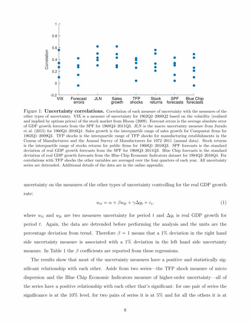
This produces 42 correlations which are plotted in Figure 1. A table of the individual correlations

is provided in the online appendix. The results show that the correlations for all measures of

uncertainty are far from one. The maximum correlation is 0.62, the mean is 0.32 and several

correlations are close to zero. Thus despite all three types of uncertainty being countercyclical,

they each fluctuate in a distinct way.

The variation in the fluctuations of the three types of uncertainty raises the question of whether

these are three independent phenomena that are all countercyclical, or whether they have a tighter

link. This is investigated by assessing whether there is a positive relationship between them that

holds above and beyond the business cycle. Specifically, the approach is to regress each measure of

7

-0.2

0

0.2

0.4

0.6

0.8

1

Co

rrela

tio

n

VIX Forecasterrors

JLN Salesgrowth

TFPshocks

Stockreturns

SPFforecasts

Blue Chipforecasts

Figure 1: Uncertainty correlations. Correlation of each measure of uncertainty with the measures of theother types of uncertainty. VIX is a measure of uncertainty for 1962Q2–2008Q2 based on the volatility (realizedand implied by options prices) of the stock market from Bloom (2009). Forecast errors is the average absolute errorof GDP growth forecasts from the SPF for 1968Q3–2011Q3. JLN is the macro uncertainty measure from Juradoet al. (2015) for 1960Q4–2016Q4. Sales growth is the interquartile range of sales growth for Compustat firms for1962Q1–2009Q3. TFP shocks is the interquartile range of TFP shocks for manufacturing establishments in theCensus of Manufacturers and the Annual Survey of Manufacturers for 1972–2011 (annual data). Stock returnsis the interquartile range of stocks returns for public firms for 1960Q1–2010Q3. SPF forecasts is the standarddeviation of real GDP growth forecasts from the SPF for 1968Q3–2011Q3. Blue Chip forecasts is the standarddeviation of real GDP growth forecasts from the Blue Chip Economic Indicators dataset for 1984Q3–2016Q4. Forcorrelations with TFP shocks the other variables are averaged over the four quarters of each year. All uncertaintyseries are detrended. Additional details of the data are in the online appendix.

uncertainty on the measures of the other types of uncertainty controlling for the real GDP growth

rate:

u1t = α + βu2t + γ∆yt + εt, (1)

where u1t and u2t are two measures uncertainty for period t and ∆yt is real GDP growth for

period t. Again, the data are detrended before performing the analysis and the units are the

percentage deviation from trend. Therefore β = 1 means that a 1% deviation in the right hand

side uncertainty measure is associated with a 1% deviation in the left hand side uncertainty

measure. In Table 1 the β coefficients are reported from these regressions.

The results show that most of the uncertainty measures have a positive and statistically sig-

nificant relationship with each other. Aside from two series—the TFP shock measure of micro

dispersion and the Blue Chip Economic Indicators measure of higher-order uncertainty—all of

the series have a positive relationship with each other that’s significant: for one pair of series the

significance is at the 10% level, for two pairs of series it is at 5% and for all the others it is at

8

1%. This indicates that there is some force in the economy beyond cyclical fluctuations that links

these types of uncertainty.

3 Model

To make sense of the facts about macro uncertainty, higher-order uncertainty, and micro disper-

sion, we need a model with uncertainty about some aggregate production-relevant outcome, a

source of belief differences, and firms that use their beliefs to make potentially heterogeneous pro-

duction decisions. To keep our message as transparent as possible, it is assumed that production

is linear in labor alone. Since TFP is the key state variable, macro uncertainty comes from un-

certainty about how productive current-period production will be (TFP). Belief differences arise

from heterogeneous signals about that TFP. To capture the idea that some, but not all, of peoples’

information comes from common sources, the TFP signals have public and private signal noise.

Finally, the model needs an exogenous shock that might plausibly affect all three uncertainties.

The model allows for three possibilities for this. One is a time-varying variance of TFP innova-

tions. The second and third are time-varying variances of public and private signal noise. This

section formalizes these assumptions and describes the model’s solution.

3.1 Environment

Time is discrete and starts in period 0. There is a unit mass of firms in the economy with each

firm comprised of a representative agent who can decide how much to work. Agent i’s utility in

period t depends on his output Qit and the effort cost of his labor Lit:

Uit = Qit − Lγit (2)

for some γ > 1. Output depends on labor effort and productivity At:

Qit = AtLit. (3)

Aggregate output is Qt ≡∫Qitdi and GDP growth is ∆qt ≡ logQt − logQt−1.

9

(a) Macro uncertainty VIX Forecast errors JLN

Micro dispersionSales growth 0.33∗∗ 0.66∗∗∗ 0.18∗∗∗

(0.15) (0.21) (0.03)TFP shock 0.94 2.27∗∗ 0.17∗

(0.60) (0.87) (0.10)Stock returns 0.77∗∗∗ 1.14∗∗∗ 0.23∗∗∗

(0.10) (0.26) (0.02)Higher-order uncertainty

SPF forecasts 0.14∗∗ 0.23∗ 0.05∗∗∗

(0.06) (0.14) (0.02)Blue Chip forecasts 0.08 −0.20 0.12∗∗∗

(0.10) (0.26) (0.02)

(b) Micro dispersion Sales growth TFP shock Stock returns

Macro uncertaintyVIX 0.08∗∗ 0.07 0.34∗∗∗

(0.04) (0.05) (0.04)Forecast errors 0.09∗∗∗ 0.07∗∗ 0.09∗∗∗

(0.03) (0.03) (0.02)JLN 0.91∗∗∗ 0.46∗ 1.38∗∗∗

(0.15) (0.26) (0.14)Higher-order uncertainty

SPF forecasts 0.13∗∗∗ −0.04 0.14∗∗∗

(0.05) (0.05) (0.04)Blue Chip forecasts 0.23∗∗∗ 0.05 0.14∗∗

(0.07) (0.08) (0.07)

(c) Higher-order uncertainty SPF forecasts Blue Chip forecasts

Macro uncertaintyVIX 0.28∗∗ 0.08

(0.11) (0.10)Forecast errors 0.07∗ −0.03

(0.04) (0.04)JLN 1.14∗∗∗ 2.07∗∗∗

(0.35) (0.35)Micro dispersion

Sales growth 0.37∗∗∗ 0.41∗∗∗

(0.13) (0.13)TFP shock −0.42 0.34

(0.51) (0.52)Stock returns 0.48∗∗∗ 0.30∗∗

(0.14) (0.14)

Table 1: Coefficients for uncertainty regressions controlling for the business cycle. Thistable shows the value of the β coefficient for the regression specified in equation (1). Standard errors are inparentheses. ∗∗∗, ∗∗ and ∗ denote significance with respect to zero at the 1%, 5% and 10% levels respectively. Alluncertainty series are detrended and put in percentage deviations from trend units. See the notes to Figure 1 fordetails of the series.

10

The growth rate of productivity at time t, ∆at ≡ log(At)− log(At−1), is:

∆at = α0 + σtεt. (4)

where εt ∼ N(0, 1) and draws are independent. The key feature of this equation is that the

variance of TFP growth, σ2t , can be time-varying. This will be one of the potential sources of

uncertainty shocks discussed in the next section.

Agent i makes his labor choice Lit at the end of period t − 1. His objective is to maximize

expected period t utility.9 The agent makes this decision at the end of period t − 1. At this

point it is assumed that the agent knows σt but εt has not yet been realized so he does not know

productivity At. This assumption holds if σ2t follows a GARCH process, for example, as it will

later in the paper.

At the end of period t − 1 each agent observes an unbiased signal about TFP growth which

has both public (common) noise and private noise:

zi,t−1 = ∆at + ηt−1 + ψi,t−1, (5)

where ηt−1 ∼ N(0, σ2ηt−1

) and ψi,t−1 ∼ N(0, σ2ψ,t−1).

10 All draws of the public and private noise

shocks, the ηt−1’s and ψi,t−1’s, are independent of each other.11 The variances of public and

private signal noises are allowed to vary over time, so they are potential sources of uncertainty

shocks. The information set of firm i at the end of period t − 1 is Ii,t−1 = {At−1, zi,t−1}, where

At−1 ≡ {A0, A1, . . . , At−1}. Agents know the history of their private signals as well, but since

signals are about Xt which is revealed after production at the end of each period,12 past signals

contain no additional relevant information.

9Decisions at time t have no effect on future utility so the agent is also maximizing expected discounted utility.10These correlated signals also allow us to investigate the extreme cases of purely public and purely private

signals. Pure public signals act just like a reduction in prior uncertainty. They can be created by setting privatesignal noise to zero σ2

ψ,t−1 = 0. Pure private signals are a special case where public signal noise (ση) is zero.11As in Lucas (1972), there is no labor market, which means that there is not a wage which agents can use to

learn about Xt or ∆at. While a perfectly competitive labor market which everyone participates in could perfectlyreveal ∆at, there are many other labor market structures with frictions in which wages would provide no signal,or a noisy signal, about ∆at (e.g., a search market in which workers and firms Nash bargain over wages). Anadditional noisy public signal would not provide much additional insight since the model already allows for publicnoise in the signals that agents receive. It would however add complexity to the model, so we close this learningchannel down. Also note that if agents traded their output, prices would not provide a useful signal about TFPgrowth because once production has occurred, agents know TFP exactly.

12An agent that knows Qit can back out Xt using the production function (3) and the productivity growthequation (4).

11

3.2 Solution to the Firm’s Problem

The first-order condition for agent i’s choice of period t labor is:

Lit =

(E[At|Ii,t−1]

γ

)1/(γ−1)

. (6)

In order to make his choice of labor the agent must forecast productivity. He forms a prior belief

about TFP growth and then updates using his idiosyncratic signal. To form his prior belief he

uses his knowledge of the mean of TFP growth in equation (4): E[∆at|At−1] = α0. The agent’s

prior belief is that ∆at is normally distributed with mean α0 and variance V [∆at|At−1] = σ2t .

At the end of period t − 1, the agent receives a signal with precision (σ2η,t−1 + σ2

ψ,t−1)−1 and

updates his beliefs according to Bayes’ law. The updated posterior forecast of TFP growth is a

weighted sum of the prior belief and the signal:

E[∆at|Ii,t−1] = (1− ωt−1)α0 + ωt−1zi,t−1, (7)

where

ωt−1 ≡ [(σ2η,t−1 + σ2

ψ,t−1)(σ−2t + (σ2

η,t−1 + σ2ψ,t−1)

−1)]−1. (8)

The Bayesian weight on new information ω is also called the Kalman gain.

The posterior uncertainty, or conditional variance is common across agents because all agents

receive signals with the same precision:

Vt−1[∆at] ≡ [σ−2t + (σ2η,t−1 + σ2

ψ,t−1)−1]−1. (9)

An agent’s expected value of the level of TFP uses the fact that At = At−1 exp(∆at):

E[At|Ii,t−1] = At−1 exp(E[∆at|Ii,t−1] +

1

2Vt−1[∆at]

). (10)

Given this TFP forecast, the agent makes his labor choice according to equation (6). The labor

choice dictates the period t growth rate of firm i, ∆qit ≡ logQit− logQi,t−1, which is ∆qit = ∆at+

1γ−1(log(E[At|Ii,t−1]) − log(E[At−1|Ii,t−2])). Integrating over all firms’ output delivers aggregate

12

output:

Qt = At

∫ (E[At|Ii,t−1]

γ

)1/(γ−1)

di. (11)

3.3 Uncertainty Measures in the Model

This subsection derives macro, micro and higher-order uncertainty in the model, highlights the

similarities and differences between them, and examines what forces make each one move.

Macro uncertainty For the model, macro uncertainty is defined to be the conditional variance

of GDP growth forecasts, which is common for all agents:

Ut ≡ V [∆qt|Ii,t−1] =(γ − 1 + ωt−1)

2σ2t σ2ψ,t−1 + (γ − 1)2σ2t σ

2η,t−1 + ω2

t−1σ2η,t−1σ

2ψ,t−1

(γ − 1)2(σ2t + σ2ψ,t−1 + σ2η,t−1). (12)

If there is a prior belief about TFP with variance σ2t and a signal with variance σ2

ψ,t−1+σ2η,t−1, then

the variance of the posterior TFP belief is σ2t (σ

2ψ,t−1 + σ2

η,t−1)/(σ2t + σ2

ψ,t−1 + σ2η,t−1). You can see

this form showing up in the first two terms of the numerator and the denominator. The difference

between Ut and the Bayesian posterior that was just discussed is that Ut is the conditional variance

of output, not of TFP. How TFP maps into output also depends on what other firms believe. Thus,

the last term of the numerator ω2t−1σ

2η,t−1σ

2ψ,t−1 represents uncertainty about how much other firms

will produce.

Higher-order uncertainty Higher-order uncertainty is measured with the cross-sectional vari-

ance of GDP growth forecasts:13

Ht ≡ V{E[∆qt|Ii,t−1]

}= σ2

ψ,t−1ω2t−1

(1 +

1

(γ − 1)[σ2ψ,t−1(σ

2t + σ2

η,t−1)−1 + 1]

)2

. (13)

Higher-order uncertainty arises because there is private signal noise (σ2ψ,t−1 > 0). The larger

private signal noise is, the more agents’ signals differ. What also matters is how much they weight

these signals in their beliefs (ω2t−1). If private signal noise is so large that the signal has almost

no information, then ω2t−1 becomes small, and beliefs converge again. The last term in the large

parentheses is the rate of transformation of belief differences in TFP to belief differences in output.

Note that higher-order uncertainty is constructed to be two-sided and symmetric. Agent i’s

uncertainty about agent j is equal to j’s uncertainty about i. In general, this need not be the

13See Section A of the online appendix for the derivation of the GDP growth forecast of an agent.

13

case. For example, in sticky information (Mankiw and Reis, 2002) or inattentiveness (Reis, 2006)

theories, information sets are nested. The agent who updated more recently knows exactly what

the other believes. But the agent who updated in the past is uncertain about what the better-

informed agent knows. If we average across all pairs of agents, then the average uncertainty about

others’ expectations would be the relevant measure of higher-order uncertainty. In such a model,

belief dispersion and higher-order uncertainty are not identical, but move in lock-step. The only

way agents can have heterogeneous beliefs, but not have any uncertainty about what others know,

is if they agree to disagree. That doesn’t happen in a Bayesian setting like this.

Micro dispersion The measure of micro dispersion for the model is the cross-sectional variance

of firm growth rates:

Dt ≡∫

(∆qit −∆qt)2di =

( 1

γ − 1

)2(ω2

t−1σ2ψ,t−1 + ω2

t−2σ2ψ,t−2), (14)

where ∆qt ≡∫

∆qitdi.14 This expression shows that micro dispersion in period t depends on the

variance of private signals (σ2ψ,t−1 and σ2

ψ,t−2), the weights that agents place on their signals in

periods t− 1 and t− 2, and the Frisch elasticity of labor supply 1/(γ − 1). Holding these weights

fixed, when private signal noise increases, firms receive more heterogeneous signals. Beliefs about

TFP growth, labor choices and output therefore become more dispersed as well. When agents

place more weight on their signals, it also generates more of this dispersion. More weight on the

t−1 signal increases dispersion in Qit while more weight on the t−2 signal increases dispersion in

Qi,t−1. Both matter for earnings growth: ∆qit = log(Qit)− log(Qi,t−1). Micro dispersion depends

on γ, the inverse elasticity of labor supply, because less elastic labor makes labor and output less

sensitive to differences in signals.

Does dispersion measure firms’ uncertainty? Micro dispersion is commonly interpreted as

a measure of the uncertainty that firms have about their own economic outcomes. The uncertainty

that firms have about their period t growth rates prior to receiving their signals in period t− 1 is

V [∆qit|At−1] = σ2t +

( 1

γ − 1

)2ω2t−1(σ

2η,t−1 + σ2

ψ,t−1). (15)

14The standard deviation is used rather than the IQR measure that is commonly used for the data since thestandard deviation is more analytically tractable.

14

This expression tells us that firms have uncertainty about their growth rates that comes from three

sources. First there is uncertainty about TFP that shows up as σ2t . A firm also has uncertainty

because it doesn’t know what signal it will receive. This generates two additional sources of

uncertainty: public signal noise (σ2η,t−1) and private signal noise (σ2

φ,t−1). The relevance of these

depends on the weight that firms place on their signals (ωt−1) and how sensitive a firm’s labor

choice is to changes in its beliefs, 1/(1− γ).

Comparing the uncertainty that a firm has about its growth (15) with the dispersion of firm

growth (14) highlights two differences. First, dispersion only captures uncertainty due to private

differences in information. Both the volatility of TFP σt and noise in signals that are pub-

licly observed ση,t−1, make firms uncertain about their growth. But neither generates dispersion.

Micro dispersion only captures uncertainty caused by idiosyncratic differences in information:

( 1γ−1)2ω2

t−1σ2ψ,t−1. Second, micro dispersion systematically overestimates this component of a firm’s

uncertainty: Dt ≥ ( 1γ−1)2ω2

t−1σ2ψ,t−1. The reason is that differences in levels of output yesterday

and differences today both contribute to dispersion in firm growth rates. But firms are not uncer-

tain about what they produced yesterday. It is only differences today that matter for uncertainty.

This shows up mathematically as ωt−2σψ,t−2 being in the expression for dispersion, but not in

the expression for uncertainty. If ωt−1σψ,t−1 and ωt−2σψ,t−2 are closely correlated then changes

in micro dispersion will be a good proxy for the part of uncertainty due to private information

shocks. But it is possible to have dispersion, without there being any uncertainty.15 Despite these

issues, this paper focuses on micro dispersion, as it allows us to speak to the existing literature.

4 What is an Uncertainty Shock?

There are various, distinct measures of uncertainty. If we want to think of uncertainty as a unified

concept that can explain many business cycle and financial facts, there needs to be a single shock

that moves all these various measures. This section explores three plausible candidates and shows

that one of them can explain the comovement of uncertainty measures in the data. In so doing,

it provides a source of unification for theories based on uncertainty shocks. The three potential

sources of changes in uncertainty in the model are: changes in the amount of public signal noise

15If there is dispersion in firm output in period t− 1 but agents have perfect information in period t (which willbe the case if σ2

t = 0 so that ωt−1 = 0) so that they all choose the same output then there will be positive microdispersion in period t yet firms will have no uncertainty about their growth rates: V [∆qit|At−1] = 0.

15

(ση,t−1), changes in private signal noise (σψ,t−1), and changes in the volatility of TFP shocks (σt).

Public signal noise shocks First consider what happens to uncertainty measures when public

signal noise rises. Public signal noise is sometimes referred to as “sender noise” because noise that

originates with the sender affects receivers’ signals all in the same way. The proofs of this and all

subsequent results are in the online appendix.

Result 1. Shocks to public signal noise can generate positive or negative covariances

between any pair of the three types of uncertainty and dispersion: Fix σt and σψ,t−1

so that they do not vary over time.16

(a) If (A.7) holds then cov(Dt,Ht) > 0 and otherwise cov(Dt,Ht) ≤ 0;

(b) If (A.9) holds then cov(Dt,Ut) < 0 and otherwise cov(Dt,Ut) ≥ 0;

(c) If σψ,t−1 is sufficiently small then cov(Ht,Ut) < 0 and if only one of conditions (A.7) and

(A.9) hold then cov(Ht,Ut) > 0.

Public signal noise lowers micro dispersion. When public signal noise increases the signals that

agents receive are less informative so they place less weight on them. This causes them to have less

dispersed beliefs about TFP growth, which results in less dispersion in their labor input choices

and less dispersion in their growth rates.

For higher-order uncertainty, public signal noise has two opposing effects. The direct effect

comes from the same channel described above. A decrease in the dispersion of beliefs about TFP

growth makes GDP growth forecasts less dispersed, which reduces higher-order uncertainty. The

indirect effect arises because when agents are forecasting GDP growth, they need to forecast the

labor input decisions of other agents, who produce that GDP. When public signal noise increases,

the average signals of others (∆at + ηt−1) are more volatile. Because one’s own signal is useful

to predict others’ signals, and those signals become more important to predict, agents weight

their own signals more. Greater weight on one’s own signals causes GDP growth forecasts to

be more dispersed and higher-order uncertainty to rise. If macro volatility is sufficiently high

relative to signal noise, then the direct effect dominates because agents are mostly concerned

about forecasting TFP growth, not others’ signals. If macro volatility is low, others’ signals

16Conditions (A.7) and (A.9) are stipulated in the online appendix

16

are important to forecast, which makes the indirect effect stronger. Thus, public signal noise

shocks can generate a positive or negative covariance between higher-order uncertainty and micro

dispersion (Result 1a).

When public signal noise increases, there are also two effects on macro uncertainty. The direct

effect is that less precise signals carry less information about TFP growth. This raises uncertainty

about GDP growth. The indirect effect comes from agents needing to forecast the actions of others,

in order to forecast their output (GDP). When public signal noise increases, agents weight their

signals less in their production decisions. Since others’ signals are unknown, less weight makes it

easier for agents to forecast each others’ decisions. This reduces uncertainty about GDP growth.

Of the two opposing effects on macro uncertainty, either can dominate: If public signal noise is

sufficiently high, then forecasting the actions of others will be very important. So the indirect

effect will dominate and macro uncertainty will decrease. If private signal noise is sufficiently low,

then all agents receive similar information, will be able to forecast each others’ actions well and

the direct effect will dominate. In this case macro uncertainty will increase. Thus micro dispersion

and macro uncertainty can be positively or negatively correlated due to shocks to public signal

noise (Result 1b).

The final part of Result 1 is about the covariance between higher-order uncertainty and macro

uncertainty. These two types of uncertainty can have either a positive or negative covariance.

There is a wedge between them because it is possible for uncertainty about TFP growth to

increase and at the same time the dispersion of beliefs to decrease. This happens when private

signal noise is low. In this case, an increase in public signal noise increases macro uncertainty

because agents have more uncertainty about TFP growth. It decreases higher-order uncertainty

because agents weight their signals less and have less dispersed beliefs about TFP growth.

Private signal noise shocks A change in private signal noise can also generate positive or

negative covariances.

Result 2. Shocks to private signal noise can generate positive or negative covariances

between any pair of the three types of uncertainty and dispersion: Fix σt and ση,t−1 so

that they do not vary over time.17

(a) If σψ,t−1 is sufficiently small then cov(Ut,Ht) > 0, cov(Ut,Dt) > 0 and cov(Ht,Dt) > 0;

17Conditions (A.10) to (A.12) are stipulated in the online appendix

17

(b) If only one of (A.11) and (A.12) holds then cov(Ut,Ht) ≤ 0;

(c) If only one of (A.10) and (A.11) holds then cov(Ut,Dt) ≤ 0;

(d) If only one of (A.10) and (A.12) holds then cov(Ht,Dt) ≤ 0.

As with public noise, private signal has two competing effects on micro dispersion. There is

more dispersion in the signals agents receive so if they hold the weight on their signals fixed they

will have more dispersed beliefs about TFP growth, which will result in higher micro dispersion.

But, because the signals are less informative agents weight them less and weight their prior beliefs

more. Since agents have common prior beliefs, this decreases the dispersion in beliefs resulting in

lower micro dispersion. Which of these forces is stronger depends on parameter values.

For higher-order uncertainty, these same two opposing forces are also at work. Recall from the

discussion of public information shocks that when agents are forecasting GDP growth they need

to forecast TFP growth as well as the actions of others. The discussion of micro dispersion tells

us how an increase in private signal noise affects the dispersion of forecasts of TFP growth. For

forecasts of other agents’ actions the two forces also work in opposite directions. The fact that

agents get signals that differ more from each other will mean that there will be greater differences

in the forecasts that agents make of each others’ actions. But since these signals are noisier agents

will weight them less, which will bring their forecasts closer.

Private signal noise affects uncertainty about TFP growth and about the actions of others,

both of which matter for macro uncertainty. The fact that agents have less precise information

increases their uncertainty about TFP growth. In terms of forecasting the actions of others, agents

will be more uncertain due to the fact that signals differ more across agents, but this is offset by

the fact that agents are weighting their signals less.

When private signal noise is sufficiently small it is the increase in the dispersion of signals

that is the dominant effect and the effects of changing signals weights are secondary. In this

case all three types of uncertainty increase when private signal noise increases, so private signal

noise shocks generate positive correlations between all three types of uncertainty and dispersion.

This is part (a) of Result 2. This is not necessarily the case though. There are conditions under

which the uncertainty and dispersion measures are negatively correlated, as provided by parts

(b)–(d) of the result. There is a wedge between macro uncertainty and micro dispersion because

an increase in private signal noise increases uncertainty about TFP growth but can increase or

18

decrease the dispersion in TFP growth forecasts. This is also the cause of the wedge between

macro uncertainty and higher-order uncertainty. There is a wedge between micro dispersion and

higher-order uncertainty because agents weight their signals differently when forecasting TFP

growth and when forecasting the actions of others. These wedges are why the different measures

of uncertainty can react in opposite ways to changes in private signal noise.

Macro volatility shocks The third possible source of uncertainty shocks is changes in the

volatility of TFP growth. Unlike the other potential sources of uncertainty shocks, this source

generates positively correlated fluctuations in macro uncertainty, higher-order uncertainty and

micro dispersion without additional conditions.

Result 3. Shocks to macro volatility generate positive covariances between all pairs

of the three types of uncertainty and dispersion: Fix ση,t−1 and σψ,t−1 so that they do not

vary over time. Then cov(Ut,Ht) > 0, cov(Ut,Dt) > 0 and cov(Ht,Dt) > 0.

When macro volatility increases agents have less precise prior information about TFP growth

and they therefore weight their signals more. Since those signals are heterogeneous this causes

their beliefs about TFP growth to be more dispersed, which results in more dispersed production

decisions and higher micro dispersion. In terms of macro uncertainty, the less precise information

about TFP growth increases macro uncertainty. Agents weighting their signals more also makes

it harder for agents to forecast the actions of others’, which further increases macro uncertainty.

Higher-order uncertainty also increases for two reasons. First the increase in dispersion of beliefs

about TFP growth that results from agents weighting their signals more increases the differences

between GDP growth forecasts. These differences also increase because agents weight their signals

more when forecasting the actions of others, so there is more divergence in these forecasts.

There are two points to take from this section. The first is that the different types of uncertainty

and dispersion are theoretically distinct. They are not mechanically linked and nor do they

naturally fluctuate together. Only one of the possible sources of uncertainty shocks necessarily

generates the positive correlation between all three types of uncertainty and dispersion that is

in the data. Therefore it is erroneous to treat these types of uncertainty and dispersion as a

single unified phenomenon, as the existing uncertainty shocks literature has tended to. If we

want to unify these various shocks then a theory that ties them together is needed. That’s the

second point: If we’re after a common origin for the various uncertainty and dispersion shocks,

19

then changes in macro volatility is a possible source. The next section evaluates whether macro

volatility is quantitatively relevant for understanding uncertainty shocks.

5 Do Macro Volatility Shocks Generate Enough Uncer-

tainty Comovement?

To develop a quantitatively viable theory, this section enriches the model from Section 3 and

calibrates it to the data. The augmented, calibrated model produces uncertainty shocks that are,

in many respects, quantitatively similar to the data.

5.1 Quantitative Model

Since the focus of this section is on assessing the quantitative potential of changes in TFP growth

volatility to explain uncertainty shocks, time variation in signal noise is turned off: σψ,t−1 = σψ

and ση,t−1 = ση for all t. To estimate TFP growth volatility, some stochastic structure is needed.

Since GARCH is common and simple to estimate, it is assumed that σ2t follows a GARCH process:

σ2t = α1 + ρσ2

t−1 + φσ2t−1ε

2t−1. (16)

where εt ∼ N(0, 1), with draws being independent.

The final modification to the model is that TFP growth is given a negatively skewed distribu-

tion. This captures the idea of disaster risk. Disaster risk is a useful ingredient because it amplifies

the uncertainty shocks and is gets their cyclicality correct. Disaster risk can amplify uncertainty

during economic downturns because disasters are more likely during these periods and they are

extreme events whose exact nature is difficult to predict. This creates a lot of scope for uncertainty

and disagreement.

To introduce non-normality into the model it is assumed that the economy has an underlying

state Xt which is subject to a non-linear transformation to generate TFP growth. Specifically,

instead of ∆at being determined by equation (4),

∆at = c+ b exp(−Xt), (17)

Xt = α0 + σtεt, (18)

20

and σ2t follows equation (16). This is the TFP growth process from the baseline model, with an

exponential transformation and a linear translation. This change of variable procedure allows our

forecasters to consider a family of non-normal distributions of TFP growth and convert each one

into a linear-normal filtering problem.18 The structural form of the mapping in (17) is dictated

by a couple of observations. First, it is a simple, computationally feasible formulation that allows

us to focus our attention on conditionally skewed distributions. Note that skewness in this model

is most sensitive to b because that parameter governs the curvature of the transformation (17) of

the normal variable. Any function with similar curvature, such as a polynomial or sine function,

would deliver a similar mechanism. Second, the historical distribution of GDP growth is negatively

skewed which can be achieved by setting b < 0. Third, Orlik and Veldkamp (2015) show how a

similar formulation reproduces important properties of the GDP growth forecasts in the Survey

of Professional Forecasters.

The signal structure for this version of the model is:

zi,t−1 = Xt + ηt−1 + ψi,t−1,

where ηt−1 ∼ N(0, σ2η) and ψi,t−1 ∼ N(0, σ2

ψ). The mechanics of learning are the same as in the

baseline model, with two exceptions: (1) agents are now learning about Xt instead of ∆at, and (2)

once they form beliefs about Xt they transform these into beliefs about ∆at with equation (17).

When discussing the quantitative results, the model presented in this section will be called the

disaster risk model and the model presented in Section 3 will be called the normal model. The

difference between these models will demonstrate the role of the skewed TFP growth distribution.

There will also be results for a version of the Section 3 model in which agents have perfect

information (ση = σψ = 0) about TFP growth, which will be called the perfect information model.

The difference between this model and the normal model will demonstrate the role of imperfect

information and learning in the results.

18It is also possible to allow the parameters of the model to be unknown, in which case agents need to estimatethem each period. This version of the model with results is in the online appendix. Adding parameter learning tothe model modestly amplifies fluctuations in uncertainty.

21

5.2 Why Disaster Risk Makes Uncertainty Countercyclical

Disasters are more likely in bad times. The heightened risk of disasters makes bad states more

uncertain times. Furthermore, disasters are hard to predict. They leave lots of scope for disagree-

ment, dispersion of beliefs and dispersion of actions. These forces make all three uncertainty and

dispersion measures countercyclical.

To formalize this argument, start with the change of variable function in equation (17), which

introduced disaster risk. When this is calibrated the coefficient b is negative, meaning that the

transformation is concave. This is driven by the fact that GDP growth is negatively skewed in the

data. A concave change of variable makes extreme, low realizations of TFP growth more likely

and makes very high realizations less likely. In other words, a concave transformation creates a

negatively skewed variable. The concavity, and thus degree of negative skewness determines the

probability of negative outlier events or, in other words, the level of disaster risk.

Disaster risk and macro uncertainty Figure 2 illustrates the effect of the concave change

of variable on uncertainty about TFP growth. It plots a mapping from X into TFP growth, ∆a.

The slope of this curve is a Radon-Nikodym derivative. For illustrative purposes, suppose for a

moment that an agent has beliefs about X that are uniformly distributed. We can represent these

beliefs by a band on the horizontal axis in Figure 2. If that band is projected onto TFP growth

(the ∆a-space), the implied uncertainty about (width of the band for) ∆a depends on the state

X. When X is high the mapping is flat and the resulting band projected on the ∆a-axis is narrow.

This means that uncertainty about TFP growth and therefore GDP growth is small, so macro

uncertainty is small. When X is low the opposite it true: the band projected on the ∆a axis is

wider and uncertainty is higher.

Recall that posterior beliefs about X are actually assumed to be normally distributed. Ac-

cording to the formula for the variance of a log-normal distribution, the variance of beliefs about

TFP growth is

V [∆at|Ii,t−1] = b2(

exp(Vt−1[Xt])− 1)

exp(Vt−1[Xt]− 2E[Xt|Ii,t−1]

).

Importantly, the source of countercyclical uncertainty appears: The agent’s uncertainty about ∆at

(conditional variance) is decreasing in his expected value of Xt.

22

State (X)0

∆a

X uncertainty

∆a uncertainty

Figure 2: Change of variable function and countercyclical uncertainty. A given amount ofuncertainty about X creates more uncertainty about TFP growth when X is low than it does when X is high.

Countercyclical uncertainty arises because, in a skewed distribution, conditional variances are

not independent of means. With normally distributed prior beliefs and signals, the variance of an

agent’s posterior beliefs would be independent of the value of his signal. Furthermore, the cross-

sectional variance of the mean posterior beliefs of agents would be independent of the state Xt.

This is no longer true when there is skewness. With negative skewness, the variance of posterior

beliefs is higher when the state is lower and there is a greater risk of a disaster.

Disaster risk, higher-order uncertainty and micro dispersion To understand the role of

disaster risk in generating micro and higher-order uncertainty shocks return to Figure 2. Because

of idiosyncratic signals there will be a distribution of beliefs about the state of the economy

each period. For getting intuition assume that this distribution is uniform and represent it with

the bands on the horizontal axis in the figure. Due to the changing slope of the change of

measure function a fixed dispersion in beliefs about the state will generate greater dispersion in

beliefs about TFP growth when the economy is performing worse (lower X). This means that

when the economy is doing poorly small differences in information and beliefs about the state

generate far more disagreement about TFP growth than when the economy is doing well. Greater

disagreement about TFP growth generates more dispersion in labor choices and firm growth

rates (micro dispersion), and more dispersion in GDP growth forecasts (higher-order uncertainty).

Again, the intuition here is that when the economy is doing badly it is more sensitive to shocks

so agents respond more to differences in information. Thus disaster risk generates fluctuations in

23

Parameter Normal Disaster riskmodel model

Disutility of labor γ 2 2Non-normality b n/a −0.0767TFP growth level (disaster risk) c n/a 0.0804TFP growth level (normal) α0 0.0034 0Mean volatility α1 2.03e-5 4.36e-4Volatility persistence ρ 0.2951 0.7419Volatility innovation variance φ 0.1789 0.1937Private signal noise σψ 0.0090 0.1106Public signal noise ση 0 0

Table 2: Parameter values for the disaster risk and normal models

micro dispersion and higher-order uncertainty beyond those coming from the learning mechanism

and these fluctuations are countercyclical.

5.3 Calibration and Simulation

The normal and disaster risk models are calibrated separately, but with the same procedure, at

a quarterly frequency with data for 1968Q4–2011Q4. The disutility of labor, γ, is calibrated

externally using existing estimates. For the disaster risk model, α0 can be normalized. The

remaining parameters for the two models are determined using simulated method of moments.

The TFP growth process is calibrated using moments of GDP growth data and the signal noises

are calibrated using moments of GDP growth forecasts (from the SPF dataset). The parameter

values are reported in Table 2 and the calibration moments are in Table 3. For the perfect

information model the same parameter values as for the normal model are used, except signal

noises are set to zero: σψ = ση = 0.

To evaluate the ability of the model to generate plausible uncertainty shocks, one empirical

measure of each type of uncertainty from Section 2 is used for comparison. For macro uncertainty

the VIX is used, for micro dispersion it is sales growth dispersion and for higher-order uncertainty it

is SPF forecasts. The model offers a direct analog to micro dispersion and higher-order uncertainty

measures. But without a financial sector the VIX cannot be computed in the model, so we compute

macro uncertainty in equation (12) and compare it with the VIX. All data are detrended in order

to abstract from changes at frequencies that this paper is not attempting to explain.19 The units

19Detrending is done using a HP filter exactly as it is done in Section 2.

24

Models Data

Normal Disaster risk(1) (2) (3)

GDP growthMean∗† 2.72 2.71 2.71Standard deviation∗† 3.68 3.76 3.42Skewness† 0.00 −0.33 −0.32Kurtosis† 3.61 4.68 5.08std(|∆qt −∆q|)∗† 2.30 2.48 2.41ac(|∆qt −∆q|)∗ 0.23 0.30 0.23

Higher-order uncertaintyMean∗† 1.50 1.45 1.54

GDP growth forecastsAverage absolute error∗† 2.14 2.01 2.23

Table 3: Calibration targets. Calibration targets for the normal model are marked with ∗’s. Calibrationtargets for the disaster risk model are marked with †’s. GDP growth forecasts are from the Survey of ProfessionalForecasters. The measure of higher order uncertainty is the standard deviation of GDP growth forecasts fromthe Survey of Professional Forecasters. The period for the GDP growth data and GDP growth forecasts data is1968Q4–2011Q4. The period for the higher-order uncertainty data is 1968Q3–2011Q3. The model samples aresimulated to be the same length as the data, as described in the online appendix.

for both the real data and the output of the model are the percentage deviation from trend. To

compute model output, moments and regression coefficients are estimated in each of the 2000

simulations, using the same number of observations for each series as in the data. The results

report the mean (and/or standard deviation) of each moment or coefficient. Further calibration

and simulation details are in the online appendix.

5.4 Quantitative Results

The model can generate shocks to uncertainty and dispersion that are quantitatively similar to

the data in terms of (i) their magnitude, (ii) their correlations with each other and (iii) their

correlations with the business cycle. For each model, Table 4 reports the standard deviation of

each uncertainty and dispersion measure, which is a measure of the size of uncertainty shocks,

and the correlation of each measure with the other measures and GDP growth.20

20The means of macro uncertainty and micro dispersion are omitted. The mean of macro uncertainty is 2.50 inthe disaster risk model and the mean of the empirical proxy is 19.12. But a comparison between these numbershas no economic meaning because the data measure, the VIX, has units that are not comparable to the model.For the mean of micro dispersion, the problem is that size, age, industry and geography, all affect firm growth.Because the model’s only source of firm heterogeneity is information, the model generates significantly less microdispersion: 0.51 in the disaster risk model, compared to 18.59 in the data, on average. The online appendix extendsthe model to match average dispersion. Because this additional complexity is not essential to our main point about

25

Models Data

Perfect info. Normal Disaster risk(1) (2) (3) (4)

(a) Macro uncertaintyStandard deviation 0 10.74 13.77 20.87Corr. with GDP growth 0 0.00 −0.19 −0.26Period 1962Q2–2008Q2

(b) Higher-order uncertaintyStandard deviation 0 18.49 22.69 31.13Corr. with GDP growth 0 0.00 −0.12 −0.28Corr. with micro uncertainty 0 0.42 0.75 0.43Corr. with macro uncertainty 0 0.99 0.98 0.24Period 1968Q3–2011Q3

(c) Micro dispersionStandard deviation 0 10.29 13.83 11.58Corr. with GDP growth 0 0.00 −0.06 −0.52Corr. with macro uncertainty 0 0.43 0.76 0.32Period 1962Q1–2009Q3

Table 4: Simulation results and data counterparts. The three models are described in Sections3 and 5. The measures of macro uncertainty, micro dispersion and higher-order uncertainty for the data are theVIX, sales growth and SPF measures described in Section 2. All results are computed using the detrended seriesjust as for the empirical analysis in Section 2. The periods are the periods for the data. The model samples aresimulated to be the same length, as described in the online appendix.

As a benchmark, column (1) reports moments for the perfect information model. Because

signals inform agents perfectly about the aggregate state Xt, they can forecast GDP growth

perfectly and there is no macro uncertainty. Since all agents have the same beliefs, there is no

higher-order uncertainty and no micro dispersion.

When learning and disaster risk are added to the model (column 3), the model generates

plausible shocks to uncertainty and dispersion. Macro uncertainty shocks are about 65% as large

as in the data, higher-order uncertainty shocks are 70% as large and micro dispersion shocks

are slightly larger than in the data. All uncertainty series are also countercyclical and positively

correlated with each other, with the magnitude of most of these correlations similar to their

empirical counterparts.

Comparing the results in columns (2) and (3) shows the separate roles that learning and

uncertainty covariance, it is suppressed in the main text. To compare other moments, all series are detrended,as described in Section 5. The mean of higher-order uncertainty is reported in Table 3 because it is a calibrationtarget.

26

Macro Higher-order Microuncertainty uncertainty dispersion

Macro uncertainty 1.64∗∗∗ 0.98∗∗∗

(0.05) (0.07)Higher-order uncertainty 0.59∗∗∗ 0.58∗∗∗

(0.02) (0.045)Micro dispersion 0.59∗∗∗ 0.97∗∗∗

(0.06) (0.11)

Table 5: Uncertainty shocks are correlated in the model, even after controlling for thebusiness cycle. These results are summary statistics for β from equation (1). The model is simulated 2000times and the regressions run for each simulation. The reported coefficients are the averages across the simulations.The numbers in parentheses are the standard deviations of the coefficients across the simulations. Significancelevels are computed using the fraction of simulations for which each coefficient is above zero. ∗∗∗, ∗∗ and ∗ denotesignificance at the 1%, 5% and 10% levels respectively (two-tail tests). Each series uses a simulation period that isanalogous to the periods that the corresponding data series covers as described in detail in the online appendix.

disaster risk play. Column (2) shows that learning alone generates 70–80% of the fluctuations in

uncertainty and dispersion of the full model and also generates most of the positive correlations

between the uncertainty and dispersion series. Adding disaster risk to the model (going from

column (2) to column (3)) amplifies the uncertainty shocks and makes them countercyclical.

How much of the relationship between uncertainty and dispersion measures can the model

explain, after controlling for the business cycle? To answer this question we perform the same

regression analysis (equation (1)) on the model output as was performed on the data in Section

2. Table 5 compares regression coefficients estimated from the model to those from the data. The

columns determine the left hand side variable and the rows are the right hand side variable. For

example, the first number in the macro uncertainty column says that when higher-order uncer-

tainty deviates from trend by 1 percentage point, macro uncertainty deviates by 0.59 percentage

points. Taken together, the results show that the model generates a positive and significant re-

lationship between all three types of uncertainty and dispersion, above and beyond the business

cycle; just as for the data.

It appears that our mechanisms—learning and disaster risk—are more than strong enough

to explain the empirical comovement of uncertainty measures. In fact weakening the relation-

ship between higher-order and micro dispersion, by adding more unpredictable variation in micro

dispersion, might offer an even better fit to the data.

27

6 Conclusions

Fluctuations in micro uncertainty, macro uncertainty and higher-order uncertainty have been used

to explain recessions, asset price drops and financial crises. While all are dubbed “uncertainty

shocks,” this paper has shown that they are distinct phenomena, both empirically and theoretically.

In order to unify them a theory is needed that explains how they are linked.

This paper has explored various possible theories and found that volatile macro outcomes create

macro uncertainty, higher-order uncertainty and micro dispersion shocks that are correlated in a

way that’s consistent with the data. The key to the mechanism is that when macro volatility

is high, public information—past outcomes—becomes a less informative predictor of the future,

relative to private information. This makes agents put less weight on public information, more

weight on private information, and leads them to disagree more. Furthermore, when weak macro

outcomes make highly uncertain disaster outcomes more likely, uncertainty of all types move in

a correlated, volatile and countercyclical way. By offering a unified explanation for the origin of

uncertainty shocks, our results provide insight into the nature of the shocks that drive business

cycles.

28

References

Angeletos, G., Collard, F., Dellas, H., 2018. Quantifying confidence. Econometrica forthcoming.

Angeletos, G., La’O, J., 2013. Sentiments. Econometrica 81 (2), 739–779.

Arellano, C., Bai, Y., Kehoe, P., 2018. Financial frictions and fluctuations in volatility. Journal of

Political Economy forthcoming.

Bachmann, R., Bayer, C., 2013. ‘Wait-and-see’ business cycles? Journal of Monetary Economics

60 (6), 704–719.

Bachmann, R., Moscarini, G., 2012. Business cycles and endogenous uncertainty, working paper,

Yale University.

Bansal, R., Shaliastovich, I., 2010. Confidence risk and asset prices. American Economic Review

100 (2), 537–541.

Basu, S., Bundick, B., 2017. Uncertainty shocks in a model of effective demand. Econometrica

85 (3), 937–958.

Benhabib, J., Liu, X., Wang, P., 2016. Endogenous information acquisition and countercyclical

uncertainty. Journal of Economic Theory 165, 601–642.

Benhabib, J., Wang, P., Wen, Y., 2015. Sentiments and aggregate demand fluctuations. Econo-

metrica 83(2), 549–585.

Bianchi, F., Ilut, C., Schneider, M., 2018. Uncertainty shocks, asset supply and pricing over the

business cycle. Review of Economic Studies 85 (2), 810–854.

Bloom, N., 2009. The impact of uncertainty shocks. Econometrica 77 (3), 623–685.

Bloom, N., Floetotto, M., Jaimovich, N., Sapora-Eksten, I., Terry, S., 2018. Really uncertain

business cycles. Econometrica 86 (3), 1031–1065.

Christiano, L., Motto, R., Rostagno, M., 2014. Risk shocks. American Economic Review 104 (1),

27–65.

29

Decker, R., D’Erasmo, P. N., Moscoso Boedo, H., 2016. Market exposure and endogenous firm

volatility over the business cycle. American Economic Journal: Macroeconomics 8 (1), 148–198.

Fajgelbaum, P., Schaal, E., Taschereau-Dumouchel, M., 2017. Uncertainty traps. Quarterly Jour-

nal of Economics 132 (4), 1641–1692.

Gilchrist, S., Sim, J., Zakrajsek, E., 2014. Uncertainty, financial frictions, and investment dynam-

ics. NBER Working Paper 20038.

Jurado, K., Ludvigson, S., Ng, S., 2015. Measuring uncertainty. American Economic Review

105 (3), 1177–1216.

Kozlowski, J., Veldkamp, L., Venkateswaran, V., 2017. The tail that wags the economy: Beliefs

and persistent stagnation. NBER Working Paper 21719.

Lucas, R., 1972. Expectations and the neutrality of money. Journal of Economic Theory 4 (2),

103–124.

Ludvigson, S., Ma, S., Ng, S., 2018. Uncertainty and business cycles: Exogenous impulse or

endogenous response?

Mankiw, N. G., Reis, R., 2002. Sticky information versus sticky prices: A proposal to replace the

New Keynesian Phillips curve. Quarterly Journal of Economics 117 (4), 1295–1328.

Nimark, K., 2014. Man-bites-dog business cycles. American Economic Review 104 (8), 2320–2367.

Ordonez, G., 2013. The asymmetric effects of financial frictions. Journal of Political Economy

121 (5), 844–895.

Orlik, A., Veldkamp, L., 2015. Understanding uncertainty shocks and the role of the black swan.

NBER Working Paper 20445.

Pastor, L., Veronesi, P., 2012. Uncertainty about government policy and stock prices. Journal of

Finance 67 (4), 1219–1264.

Reis, R., 2006. Inattentive producers. Review of Economic Studies 73 (3), 793–821.

Schaal, E., 2017. Uncertainty and unemployment. Econometrica 85 (6), 1675–1721.

30

Van Nieuwerburgh, S., Veldkamp, L., 2006. Learning asymmetries in real business cycles. Journal

of Monetary Economics 53(4), 753–772.

31

What Are Uncertainty Shocks?

Online Appendix

Contents

A Theoretical Appendix 1A.1 GDP Forecasts . . . . . . . . . . . . . . . . . . . . . . . . . . . . . . . . . . . . . . . . . . . . . . 1A.2 Proofs of Results . . . . . . . . . . . . . . . . . . . . . . . . . . . . . . . . . . . . . . . . . . . . . 2

B Additional Empirical Details 4

C Calibration and Simulation Details 5

D Extension with Parameter Learning 7

E Extension with Additional Firm Heterogeneity 9

A Theoretical Appendix

A.1 GDP Forecasts

This section derives GDP and GDP growth forecasts, which are used in Section 4 and for computing thequantitative results.

Using equation (10) and the fact that TFP growth forecasts are normally distributed in the cross section, itfollows from equation (11) that:

Qt = Atγ1/(1−γ) exp

[1

γ − 1

(logAt−1 + (1− ωt−1)E[∆at|At−1] + ωt−1(∆at + ηt−1)

+ω2t−1σ

2ψ

2(γ − 1)+

1

2Vt−1[∆at]

)]. (A.1)

Note that ω2t−1σ

2ψ is the cross-sectional variance of firms forecasts of TFP growth in period t. Separating the

terms in equation (A.1) that are known at the end of period t− 1 from those that are unknown,

Qt = Γt−1 exp[f(∆at, ηt−1)], (A.2)

where f(∆at, ηt−1) ≡ ∆at + (ωt−1

γ−1 )(∆at + ηt−1) and

Γt−1 ≡ γ1/(1−γ)At−1 exp

[1

γ − 1

(logAt−1 + (1− ωt−1)E[∆at|At−1] +

ω2t−1σ

2ψ

2(γ − 1)+Vt−1[∆at]

2

)].

Now consider agent i’s forecast of GDP. Under agent i’s beliefs at the end of period t − 1, ∆at + ηt−1 isnormally distributed. Therefore f(∆at, ηt−1) is normally distributed under these beliefs so agent i’s forecast ofperiod t GDP can be expressed as

E[Qt|Ii,t−1] = Γt−1 exp(E[f(∆at, ηt−1)|Ii,t−1] +

1

2V [f(∆at, ηt−1)|Ii,t−1]

). (A.3)

1

Evaluating E[f(∆at, ηt−1)|Ii,t−1] requires the mean of agent i’s posterior belief about ∆at + ηt−1. This can becomputed by Bayes’ law:

E[∆at + ηt−1|Ii,t−1] =(σ2t + σ2

η)−1E[∆at|At−1] + σ−2ψ zi,t−1

(σ2t + σ2

η)−1 + σ−2ψ.

Therefore

E[f(∆at, ηt−1)|Ii,t−1] = (1− ωt−1)E[∆at|At−1] + ωt−1zi,t−1

+( ωt−1γ − 1

)( (σ2t + σ2

η)−1E[∆at|At−1] + σ−2ψ zi,t−1

(σ2t + σ2

η)−1 + σ−2ψ

). (A.4)

Let Λt ≡ [∆at − E[∆at|At−1], ηt−1]′. Then the variance term in equation (A.3) is

V [f(∆at, ηt−1)|Ii,t−1] =[(

1 + ωt−1

γ−1

)ωt−1

γ−1

]V [Λt|Ii,t−1]

[(1 + ωt−1

γ−1

)ωt−1

γ−1

]′(A.5)

where

V [Λt|Ii,t−1] =

[σ2t 0

0 σ2η

]−[σ2t

σ2η

](σ2t + σ2

ψ + σ2η)−1

[σ2t σ2

η

]. (A.6)

Together equations (A.3), (A.4), (A.5) and (A.6) define agent i’s forecast of period t GDP.The GDP growth forecast of agent i is

E[∆qt|Ii,t−1] = E[f(∆at, ηt−1)|Ii,t−1] + log Γt−1 + logQt−1.

The expectation can be computed using equation (A.4).

A.2 Proofs of Results

Proof of Result 1 To prove this result we use the derivatives of Ut, Ht and Dt with respect to σ2η,t−1 since

these derivatives have the same sign as the derivative with respect to ση,t−1 and it simplifies the math. Toshow that ∂Dt/∂ση,t−1 < 0 partial differentiate equation (14) with respect to σ2

η,t−1 and use the fact that∂ωt−1/∂σ

2η,t−1 < 0 from equation (8).

For the effect of public signal noise on higher-order uncertainty start by taking the partial derivative∂Ht/∂σ2

η,t−1 and dropping terms that are not needed to sign the derivative. To simplify notation from nowon drop the time subscripts from ωt−1, ση,t−1 and σψ,t−1. Then

sgn

{∂Ht∂σ2

η

}= sgn

∂ω

∂σ2η

(1 +

1

(γ − 1)[σ2ψ(σ2

t + σ2η)−1 + 1]

)+ω(γ − 1)σ2

ψ

(σ2t + σ2

η)2

(1

(γ − 1)[σ2ψ(σ2

t + σ2η)−1 + 1]

)2

where sgn{·} is the signum function that extracts the sign of a real number. Computing ∂ω/∂σ2η, substituting

in the expressions for this and ω and dropping more terms that are not needed to sign the derivative gives

sgn

{∂Ht∂σ2

η

}= sgn

{− σ4

t

σ2t + σ2

η + σ2ψ

(1 +

1

(γ − 1)[σ2ψ(σ2

t + σ2η)−1 + 1]

)

+σ2ψ

(σ2t + σ2

η)2

(1

(γ − 1)[σ2ψ(σ2

t + σ2η)−1 + 1]2

)}

= sgn

{−σ4t

((γ − 1)[σ2

ψ(σ2t + σ2

η)−1 + 1] + 1)

σ2t + σ2

η + σ2ψ

+σ2ψ

(σ2t + σ2

η)[σ2ψ + σ2

t + σ2η]

}

= sgn

{−σ4

t

((γ − 1)[σ2

ψ(σ2t + σ2

η)−1 + 1] + 1)

+σ2ψ

σ2t + σ2

η

}.

2

Therefore ∂Ht/∂σ2η < 0 if

σ4t

((γ − 1)[σ2

ψ(σ2t + σ2

η)−1 + 1] + 1)>

σ2ψ

σ2t + σ2

η

. (A.7)

Part (a) of Result 1 follows from this condition. Since γ > 1 a sufficient condition for this to hold is

σ4t >

σ2ψ

σ2t + σ2

η

. (A.8)

For macro uncertainty, taking the partial derivative with respect to σ2η and dropping terms that are not

needed to sign this derivative gives

sgn

{∂Ut∂σ2

η

}= sgn

{(γ − 1)2σ4

t + ω2σ4ψ − 2ωσ2

t σ2ψ[(γ − 1 + ω)σ2

t (σ2t + σ2

ψ + σ2η) + (γ − 1)]

}.

Therefore ∂Ut/∂σ2η > 0 if

(γ − 1)2σ4t + ω2σ4

ψ > 2ωσ2t σ

2ψ[(γ − 1 + ω)σ2

t (σ2t + σ2

ψ + σ2η) + (γ − 1)]. (A.9)

Part (b) of Result 1 follows from this condition. A sufficient condition for this to hold is that σ2ψ is sufficiently

small:

limσ2ψ→0

sgn

{∂Ut∂σ2

η

}= sgn

{(γ − 1)2σ4

t

}.

Observe that in the limit as σ2ψ → 0 the condition in equation (A.8) is also satisfied. Therefore in this case

cov(Ut,Ht) < 0, which proves the first part of Result 1(c). The second part of result 1(c) follows directly fromconditions (A.7) and (A.9).

Proof of Result 2 To prove this result we use the derivatives of Ut, Ht and Dt with respect to σ2ψ,t−1 since

these derivatives have the same sign as the derivative with respect to σψ,t−1 and it simplifies the math. As forthe proof of Result 1 drop the t− 1 subscripts on ω, σψ and ση.

Taking the partial derivative of Dt with respect to σ2ψ,t−1 and dropping terms that are not need to sign the

derivative gives

sgn

{∂Dt∂σ2

ψ

}= sgn

{1−

2σ2ψ

σ2η + σ2

ψ + σ2t

}.

Therefore ∂Dt/∂σ2ψ > 0 if

1 >2σ2

ψ

σ2η + σ2

ψ + σ2t

. (A.10)

For macro uncertainty, taking the partial derivative and dropping terms that are not needed to sign thederivative gives

sgn

{∂Ut∂σ2

ψ

}= sgn

{2(γ − 1 + ω)

∂ω

∂σ2ψ

σ2t σ

2ψ(σ2

t + σ2ψ + σ2

η) + (γ − 1)2σ4t

+ 2(γ − 1)ωσ2t (σ2

t + σ2η) + ω2(σ2

t + σ2η)2}.

Using the fact that ∂ω/∂σ2ψ = −σ−2t ω2 this simplifies to

sgn

{∂Ut∂σ2

ψ

}= sgn

{(γ − 1)2σ4

t + 2(γ − 1)ωσ2t (σ2

t + σ2η) + ω2(σ2

t + σ2η)2 − 2(γ − 1 + ω)ωσ2

ψ(σ2t + σ2

ψ + σ2η)}.

Therefore ∂Ut/∂σ2ψ > 0 if

(γ − 1)2σ4t + 2(γ − 1)ωσ2

t (σ2t + σ2

η) + ω2(σ2t + σ2

η)2 > 2(γ − 1 + ω)ωσ2ψ(σ2

t + σ2ψ + σ2

η). (A.11)

3

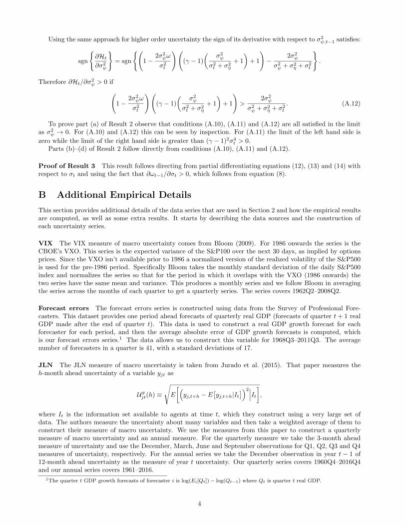
Using the same approach for higher order uncertainty the sign of its derivative with respect to σ2ψ,t−1 satisfies:

sgn

{∂Ht∂σ2

ψ

}= sgn

{(1−

2σ2ψω

σ2t

)((γ − 1)

(σ2ψ

σ2t + σ2

η

+ 1

)+ 1

)−

2σ2ψ

σ2ψ + σ2

η + σ2t

}.

Therefore ∂Ht/∂σ2ψ > 0 if(

1−2σ2

ψω

σ2t

)((γ − 1)

(σ2ψ

σ2t + σ2

η

+ 1

)+ 1

)>

2σ2ψ

σ2ψ + σ2

η + σ2t

. (A.12)

To prove part (a) of Result 2 observe that conditions (A.10), (A.11) and (A.12) are all satisfied in the limitas σ2

ψ → 0. For (A.10) and (A.12) this can be seen by inspection. For (A.11) the limit of the left hand side is

zero while the limit of the right hand side is greater than (γ − 1)2σ4t > 0.

Parts (b)–(d) of Result 2 follow directly from conditions (A.10), (A.11) and (A.12).

Proof of Result 3 This result follows directing from partial differentiating equations (12), (13) and (14) withrespect to σt and using the fact that ∂ωt−1/∂σt > 0, which follows from equation (8).

B Additional Empirical Details

This section provides additional details of the data series that are used in Section 2 and how the empirical resultsare computed, as well as some extra results. It starts by describing the data sources and the construction ofeach uncertainty series.

VIX The VIX measure of macro uncertainty comes from Bloom (2009). For 1986 onwards the series is theCBOE’s VXO. This series is the expected variance of the S&P100 over the next 30 days, as implied by optionsprices. Since the VXO isn’t available prior to 1986 a normalized version of the realized volatility of the S&P500is used for the pre-1986 period. Specifically Bloom takes the monthly standard deviation of the daily S&P500index and normalizes the series so that for the period in which it overlaps with the VXO (1986 onwards) thetwo series have the same mean and variance. This produces a monthly series and we follow Bloom in averagingthe series across the months of each quarter to get a quarterly series. The series covers 1962Q2–2008Q2.

Forecast errors The forecast errors series is constructed using data from the Survey of Professional Fore-casters. This dataset provides one period ahead forecasts of quarterly real GDP (forecasts of quarter t+ 1 realGDP made after the end of quarter t). This data is used to construct a real GDP growth forecast for eachforecaster for each period, and then the average absolute error of GDP growth forecasts is computed, whichis our forecast errors series.1 The data allows us to construct this variable for 1968Q3–2011Q3. The averagenumber of forecasters in a quarter is 41, with a standard deviations of 17.

JLN The JLN measure of macro uncertainty is taken from Jurado et al. (2015). That paper measures theh-month ahead uncertainty of a variable yjt as

Uyjt(h) ≡

√E

[(yj,t+h − E

[yj,t+h|It

])2∣∣∣It],where It is the information set available to agents at time t, which they construct using a very large set ofdata. The authors measure the uncertainty about many variables and then take a weighted average of them toconstruct their measure of macro uncertainty. We use the measures from this paper to construct a quarterlymeasure of macro uncertainty and an annual measure. For the quarterly measure we take the 3-month aheadmeasure of uncertainty and use the December, March, June and September observations for Q1, Q2, Q3 and Q4measures of uncertainty, respectively. For the annual series we take the December observation in year t − 1 of12-month ahead uncertainty as the measure of year t uncertainty. Our quarterly series covers 1960Q4–2016Q4and our annual series covers 1961–2016.

1The quarter t GDP growth forecasts of forecaster i is log(Ei[Qt]) − log(Qt−1) where Qt is quarter t real GDP.

4

Micro dispersion measures The three measures of micro dispersion—the sales growth, stock return andTFP shocks series—are all taken from Bloom et al. (2018). Full details of these series are provided in that paper,so a brief summary is sufficient here. The sales growth series is the interquartile range of firm sales growthcomputed using data on all public firms with at least 100 quarters of data in Compustat between 1962 and 2010.The sample contains 2,465 firms. The growth rate of firm i in quarter t is measured as

Qi,t+4 −Qit12 (Qi,t+4 +Qit)

, (B.1)

where Qit is the sales of firm i in quarter t. This series is quarterly and covers 1962Q1–2009Q3. The stock returnsseries is the interquartile range of monthly stock returns for all public firms with at least 25 years of data inCRSP between 1960 and 2010. We make the series quarterly by averaging it across the three months within eachquarter. The series covers 1960Q1–2010Q3. The TFP shocks series is constructed using data on establishmentswith at least 25 years of observations in the Census of Manufacturers or Annual Survey of Manufacturers fromthe U.S. Census Bureau. There are 15,673 establishments in the sample and the data is annual covering 1972–2011. TFP of establishment j (zj,t) is measured using the method from Foster et al. (2001) and TFP shocks aremeasured as the residuals from:

log(zj,t) = ρ log(zj,t−1) + µj + λt + ej,t,

where µj and λt are establishment and time fixed effects, respectively. The TFP shocks uncertainty series isthe interquartile range of these TFP shocks. Census of Manufacturers year fixed effects are removed from theseries by regressing it on a constant and a dummy variable for each year in which these Censuses occur, andsubtracting the Census year effect from the observation for the relevant year.

SPF forecasts The SPF forecasts series is constructed using the same data from the Survey of ProfessionalForecasters as the forecast errors series. This series is constructed by computing the standard deviation of realGDP growth forecasts for each quarter. The forecast for quarter t GDP growth is made at the end of quartert− 1. The series covers 1968Q3–2011Q3.

Blue Chip forecasts The Blue Chip forecasts series is constructed using data from the Blue Chip EconomicIndicators dataset. Like the Survey of Professional Forecasters this dataset provides real GDP growth forecastsmade by professional forecasters. This data is used to compute the standard deviation of forecasts of real GDPgrowth for each quarter, with the forecasts made at the start of the quarter. The series covers 1984Q3 to 2016Q4.

Additional details for empirical analysis The main body of the paper presents results on the correlationsbetween the uncertainty series and regressions of the series on each other controlling for GDP growth. The full setof correlation results are provided in Table 1. For both the correlation and regression analysis it is necessary toensure that the various series are measuring uncertainty over the same horizon. For correlations and regressionsthat use pairs from the following uncertainty series no adjustments are required as they all measure uncertaintyover a one quarter horizon: VIX, forecasts erros, JLN uncertainty, stock returns, SPF forecasts and Blue Chipforecasts. For correlations and regressions using one of these six series and the sales growth dispersion measurean adjustment is needed because sales growth dispersion is computed using sales growth over four quarters. Theother series are adjusted to match up with the horizon of sales growth by averaging them over the same fourquarters that sales growth is measured over.

The TFP shocks series measures micro dispersion over an annual horizon. The make the horizon of the sixquarterly series match up with this they are averaged over the 4 quarters of each year. To match the horizon ofthe sales growth series with this the observation for the last quarter of year t − 1 (which uses growth over thesubsequent four quarters) is used to measure dispersion for year t.

As noted in the text, for all of the regressions and correlations the series are detrended using a HP filter. Foranalysis at quarterly and annual frequencies the smoothing parameter is equal to 1600 and 100, respectively.

C Calibration and Simulation Details

Disaster risk model calibration The disaster risk model has nine parameters: a parameter controlling thedisutility of labor (γ), a parameter for the level of TFP growth (c), a parameter controlling the curvature of thechange of measure function (b), four parameters for the Xt process (α0, α1, ρ and φ), and public and private

5

(a) Macro uncertainty VIX Forecast errors JLN

Micro dispersionSales growth 0.27 0.30 0.62TFP shock 0.34 0.42 0.39Stock return 0.56 0.27 0.50

Higher-order uncertaintySPF forecasts 0.34 0.14 0.30Blue Chip forecasts 0.10 −0.04 0.43

(b) Micro dispersion Sales growth TFP shocks Stock returns

Macro uncertaintyVIX 0.27 0.34 0.56Forecast errors 0.30 0.42 0.27JLN 0.62 0.39 0.50

Higher-order uncertaintySPF forecasts 0.43 0.04 0.33Blue Chip forecasts 0.49 0.26 0.21

(c) Higher-order uncertainty SPF forecasts Blue Chip forecasts

Macro uncertaintyVIX 0.34 0.10Forecast errors 0.14 −0.04JLN 0.30 0.43

Micro dispersionSales growth 0.43 0.49TFP shock 0.04 0.26Stock return 0.33 0.21

Table 1: Uncertainty correlations. Correlations of each measure of uncertainty with the measures of the other types ofuncertainty. Each series is described in detail in Section B of this appendix. All uncertainty series are detrended.

signal noise (ση and σψ respectively). γ is set to 2, which corresponds to a Frisch labor supply elasticity of one.This is within the range of Frisch elasticities that Keane and Rogerson (2015) argue are reasonable at the macrolevel. α0 can be normalized and is set to 0. The remaining parameters are calibrated to target seven momentsof the data for 1968Q4–2011Q4: the mean, standard deviation, skewness and kurtosis of GDP growth (all realGDP); the standard deviation of the absolute difference between GDP growth and its mean, std(|∆qt − ∆q|)where ∆q is average GDP growth for the sample; the average cross-sectional standard deviation of GDP growthforecasts; and the average (over forecasters and over time) absolute error of GDP growth forecasts, which is

1

T

T∑t=1

1

Nt

∑i∈It

|E[∆qt|Ii,t−1]−∆qt|, (C.1)

where T is the number of periods in the data. The forecast data for the calibration is taken from the Survey ofProfessional Forecasters.

The calibration targets moments of GDP growth rather than moments of TFP growth because the forecastdata is for GDP growth, so we want the GDP growth process in the model to match the data, even if the produc-tion economy is simple. Matching forecast dispersion ensures that the mean level of higher-order uncertainty iscorrect, but leaves fluctuations in higher-order uncertainty as a free moment. Likewise, the average absolute fore-cast error is related to the average amount of macro uncertainty, but does not discipline the uncertainty shocks.Thus the calibration strategy allows the time variation in all three types of uncertainty, their correlations withthe business cycle and their correlations with each other to be endogenously determined.

The calibration procedure is simulated method of moments. The objective is to minimize the sum of squaredpercentage deviations of the model moments from their data counterparts. To attain this objective functionthe moment conditions are divided by the value of the relevant moment of the data and the weighting matrixis the identity matrix. The moments of the model are calculated by simulating it 2000 times, calculating themoments of the model for each simulation and then averaging each moment across the simulations. For eachsimulation the moments are computed using the the same number of periods of observations as the data that isbeing matched has (173 periods for 1968Q4–2011Q4) so that model and data are comparable. Each simulationconsists of: simulating Xt for an initial burn in period; simulating the Xt process for 173 periods that will be

6

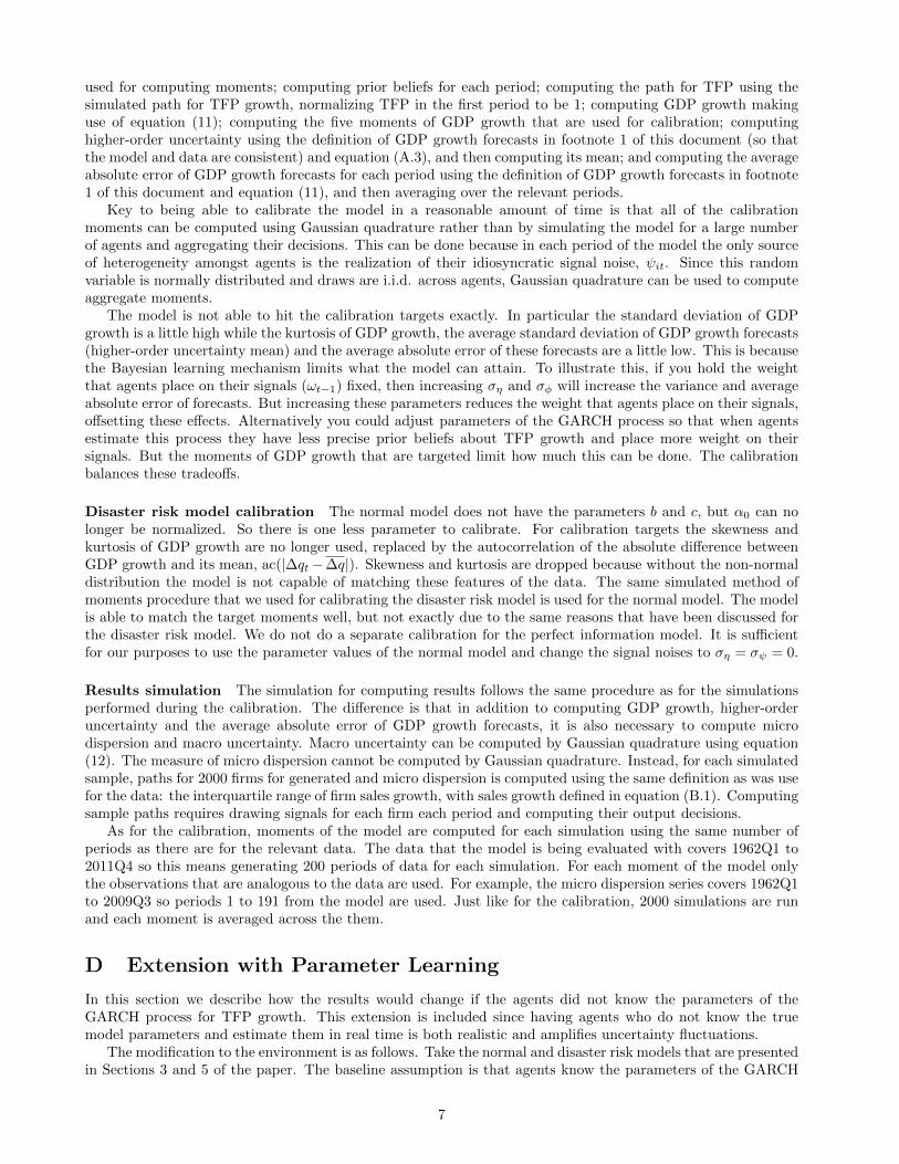
used for computing moments; computing prior beliefs for each period; computing the path for TFP using thesimulated path for TFP growth, normalizing TFP in the first period to be 1; computing GDP growth makinguse of equation (11); computing the five moments of GDP growth that are used for calibration; computinghigher-order uncertainty using the definition of GDP growth forecasts in footnote 1 of this document (so thatthe model and data are consistent) and equation (A.3), and then computing its mean; and computing the averageabsolute error of GDP growth forecasts for each period using the definition of GDP growth forecasts in footnote1 of this document and equation (11), and then averaging over the relevant periods.

Key to being able to calibrate the model in a reasonable amount of time is that all of the calibrationmoments can be computed using Gaussian quadrature rather than by simulating the model for a large numberof agents and aggregating their decisions. This can be done because in each period of the model the only sourceof heterogeneity amongst agents is the realization of their idiosyncratic signal noise, ψit. Since this randomvariable is normally distributed and draws are i.i.d. across agents, Gaussian quadrature can be used to computeaggregate moments.

The model is not able to hit the calibration targets exactly. In particular the standard deviation of GDPgrowth is a little high while the kurtosis of GDP growth, the average standard deviation of GDP growth forecasts(higher-order uncertainty mean) and the average absolute error of these forecasts are a little low. This is becausethe Bayesian learning mechanism limits what the model can attain. To illustrate this, if you hold the weightthat agents place on their signals (ωt−1) fixed, then increasing ση and σφ will increase the variance and averageabsolute error of forecasts. But increasing these parameters reduces the weight that agents place on their signals,offsetting these effects. Alternatively you could adjust parameters of the GARCH process so that when agentsestimate this process they have less precise prior beliefs about TFP growth and place more weight on theirsignals. But the moments of GDP growth that are targeted limit how much this can be done. The calibrationbalances these tradeoffs.

Disaster risk model calibration The normal model does not have the parameters b and c, but α0 can nolonger be normalized. So there is one less parameter to calibrate. For calibration targets the skewness andkurtosis of GDP growth are no longer used, replaced by the autocorrelation of the absolute difference betweenGDP growth and its mean, ac(|∆qt−∆q|). Skewness and kurtosis are dropped because without the non-normaldistribution the model is not capable of matching these features of the data. The same simulated method ofmoments procedure that we used for calibrating the disaster risk model is used for the normal model. The modelis able to match the target moments well, but not exactly due to the same reasons that have been discussed forthe disaster risk model. We do not do a separate calibration for the perfect information model. It is sufficientfor our purposes to use the parameter values of the normal model and change the signal noises to ση = σψ = 0.

Results simulation The simulation for computing results follows the same procedure as for the simulationsperformed during the calibration. The difference is that in addition to computing GDP growth, higher-orderuncertainty and the average absolute error of GDP growth forecasts, it is also necessary to compute microdispersion and macro uncertainty. Macro uncertainty can be computed by Gaussian quadrature using equation(12). The measure of micro dispersion cannot be computed by Gaussian quadrature. Instead, for each simulatedsample, paths for 2000 firms for generated and micro dispersion is computed using the same definition as was usefor the data: the interquartile range of firm sales growth, with sales growth defined in equation (B.1). Computingsample paths requires drawing signals for each firm each period and computing their output decisions.

As for the calibration, moments of the model are computed for each simulation using the same number ofperiods as there are for the relevant data. The data that the model is being evaluated with covers 1962Q1 to2011Q4 so this means generating 200 periods of data for each simulation. For each moment of the model onlythe observations that are analogous to the data are used. For example, the micro dispersion series covers 1962Q1to 2009Q3 so periods 1 to 191 from the model are used. Just like for the calibration, 2000 simulations are runand each moment is averaged across the them.

D Extension with Parameter Learning

In this section we describe how the results would change if the agents did not know the parameters of theGARCH process for TFP growth. This extension is included since having agents who do not know the truemodel parameters and estimate them in real time is both realistic and amplifies uncertainty fluctuations.

The modification to the environment is as follows. Take the normal and disaster risk models that are presentedin Sections 3 and 5 of the paper. The baseline assumption is that agents know the parameters of the GARCH

7

process for the variance of Xt: α0, α1, ρ and φ in equation (16). This assumption is now dropped.2 Agentstherefore need to estimate these parameters in order to form beliefs about TFP growth. Specifically the processfor forming beliefs at the end of period t − 1 is as follows. Using the observed history of TFP, At−1, agentsestimate the process for ∆at (Xt for the disaster risk model) by maximum likelihood and based on the parameterestimates from this they form their prior beliefs about ∆at (Xt). These beliefs are normally distributed withmean E[∆at|At−1] (E[Xt|At−1]) and variance vt−1 = V [∆at|At−1] (vt−1 = V [Xt|At−1]). Given these priors theagents then update their beliefs using their signals in the same way as in the model presented in the paper, thatis according to equations (7) and (9).

Dropping the assumption that the parameters of the GARCH process are known adds additional scope forprior beliefs to fluctuate over time. Shocks to ∆at (Xt) will now not only affect its future variance through theGARCH process, but will cause agents to re-estimate the parameters of the process. As the estimated parameterschange agents beliefs about future values of ∆at (Xt) will change, which is an additional source of uncertaintyshocks. Note that conditional on the sequence of prior beliefs, the model with parameter learning is identicalto the model used in the quantitative exercise in the paper. Thus uncertainty shocks due to changes in beliefsabout parameters have the same qualitative effects as uncertainty shocks due to changes in σt in the model inwhich parameters are known. The question is how much parameter learning changes the magnitude of shocksto the economy.

To assess the quantitative contribution of parameter learning to the results the quantitative exercise fromthe body of the paper is repeated for this extension of the model. Before presenting the results there are a fewcomments to make on how the quantitative exercise with parameter learning is performed. When this model issolved numerically two simplifying assumptions are made. First, when agents estimate the TFP process and usethe estimate to construct prior beliefs about TFP growth, they would optimally consider the whole distributionof possible parameter values, conditional on the data set. For this they would require Bayesian Monte Carlomethods to estimate the parameters. For the number of parameters that have to be estimated each period thisprocedure is quite slow. Therefore the solution is approximated by replacing the distribution of each parameterwith its mean—the maximum likelihood estimate. This understates uncertainty slightly. However, experimentswith lower-parameter versions of the model show that uncertainty fluctuations are quite similar in the true andapproximate models. Second, zero weight is put on heterogeneous signals when estimating parameters. This isdone because if estimated distributions differ across agents then keeping track of the distribution of distributionsis too memory-intensive. The quantitative effect is tiny because the data history is a long string of public signalsand the private signal is only one noisy piece of information. The weights agents place on the heterogeneoussignals would typically be less than one percent and thus create very small differences in beliefs. Experimentswith fewer agents and periods confirm that this heterogeneous parameter effect is negligible.

For the calibration of the models with parameter learning the same parameters are used as for the modelsin the body of the paper. This approach is taken since the calibration moments of the models change negligiblywhen parameter learning is added to the model. For simulating the model to compute results it is importantthat the model is simulated for the same length of time as the data so that agents have access to the sameamount of information for estimating parameters. Agents are assumed to have access to post-war data so eachsimulation of the model is for 259 periods, corresponding to 1947Q2 to 2011Q4. The moments of the data thatare used for assessing the model cover 1962Q1–2011Q4. This means that for the first period in which results arecomputed agents are given the previous 59 periods of data (corresponding to 1947Q2–1961Q4) to estimate theGARCH process with, and each period after that they get one additional period of data.

The results for these models are presented in Table 2, along with the results for the models without parameterlearning for comparison. First look at the results for the normal model, in columns (1) and (2) of the table. Incolumn (1) parameter learning is off and in column (2) it is turned on. Comparing the results in these columnsshows that the main function of parameter learning is to generate additional uncertainty shocks. The standarddeviations of micro dispersion, higher-order uncertainty and macro uncertainty increase by 14%, 8% and 11%,respectively, when parameter updating is turned on. The results for the two versions of the disaster risk model,presented in columns (3) and (4) of Table 2, tell the same story. Turning parameter learning on increases thestandard deviations of micro dispersion, higher-order uncertainty and macro uncertainty by 9%, 9% and 10%,respectively.

2It is still assumed that agents know the values of parameters b and c so that the model is computationally feasible. Calibratingthe model requires simulating it each time the parameters are adjusted and this requires estimating the process for Xt 400,000times. When b and c are known, this can be done efficiently using maximum likelihood techniques. Assuming agents do not know band c so that their beliefs about them change over time creates an additional source of time-variation in disaster risk that amplifiesuncertainty shocks. Results are available on request.

8

Model Normal Disaster risk

Parameter updating Off On Off On(1) (2) (3) (4)

(a) Macro uncertaintyStandard deviation 10.74 11.93 13.77 15.15Corr. with GDP growth 0.00 0.00 −0.19 −0.18Period 1962Q2–2008Q2

(b) Higher-order uncertaintyStandard deviation 18.49 19.99 22.69 24.68Corr. with GDP growth 0.00 0.00 −0.12 −0.12Corr. with Micro Unc. 0.42 0.43 0.75 0.68Corr. with Macro Unc. 0.99 0.99 0.98 0.98Period 1968Q3–2011Q3

(a) Micro dispersionStandard deviation 10.29 11.68 13.83 15.08Corr. with GDP growth 0.00 0.00 −0.06 −0.06Corr. with Macro Unc. 0.43 0.44 0.76 0.68Period 1962Q1–2009Q3

Table 2: Separating the roles of state uncertainty and parameter updating. The three models are describedin Sections 3 and 5. All results are computed using the detrended series just as for the empirical analysis in Section 2. Parameterupdating off means that agents know the values of α0, α1, ρ and φ. When it is off agents don’t know these parameters and estimatethem each period. The periods are the periods for the data. The model samples are simulated to be the same length, as describedin the appendix.

E Extension with Additional Firm Heterogeneity

This section addresses the inability of the models presented in the main text to match the mean level of microdispersion that is observed in the data. An extension of the normal model is developed for this purpose. We usethe normal model rather than the disaster risk model to reduce the burden of the calibration. While this meansthat the model will not match all of the uncertainty moments of interest it will be sufficient to demonstrate themain point of this section: that our model can be extended to match the mean level of micro dispersion.

The change to the model is to modify the TFP growth process to allow for additional heterogeneity amongstfirms. Specifically, TFP is assumed to be idiosyncratic and to follow the process:

∆ait = αit + θiσtεt, (E.1)

where αit ∼ N(α0, σ2α) and is i.i.d. across agents and over time, θi ∼ N(1, σ2

θ) and is i.i.d. across agents andσt follows the same process as in equation (16). This TFP growth process contains two changes relative to thenormal model in the main text. θi captures the idea that firms differ in their sensitivity to aggregate shocks.This sensitivity is firm specific and fixed over time. The fact that αit is now a random variable rather than aconstant captures the idea that firms experience transitory idiosyncratic shocks in addition to being affected byaggregate shocks. To maintain the learning structure of the model signals are now

zi,t−1 = σtεt + ηt−1 + ψi,t−1,

and the remainder of the model is exactly the same as in Section 3.This model has two more parameters to calibrate than the normal model. These are the variance of transitory

idiosyncratic shocks, σ2α, and the variance of firm sensitivity to aggregate shocks, σ2

θ . The targets that are usedfor these parameters are the mean and standard deviation of micro dispersion. The rest of the calibration targetsare the same as for the normal model. The calibration procedure is identical to that for the normal model withtwo exceptions: micro dispersion must be computed and this is done in the same way as described earlier in thisappendix; and since this model is much more computationally intensive than the standard model 20 simulatedsamples are generated instead of 2000. Tests show that increasing the number of samples does not significantlyaffect the results.

The parameter values are presented in Table 3 and the results in Table 4. The results show that themodel is capable of matching the mean and standard deviation of micro dispersion and simultaneously generates

9

Parameter Value

TFP growth level α0 0.0048Std. transient idiosyncratic shocks σα 0.1459Std. sensitivity to aggregate shocks σθ 4.9414Mean volatility α1 5.59e-7Volatility persistence ρ 0.1179Volatility innovation variance φ 0.0086Private signal noise σψ 0.0020Public signal noise ση 0.0061

Table 3: Parameter values for the extended model

Extended DataModel

Micro dispersionMean 14.21 18.59Standard deviation 11.11 11.58Corr. with GDP growth 0.02 −0.52Corr. with Higher-order Unc. 0.02 0.43Period 1962Q1–2009Q3

Table 4: Simulation results for extended model and data counterparts. Micro dispersion is measured withthe sales growth series that is described in Section B of this appendix. The mean of micro dispersion is computed using the rawdata. The rest of the results are computed using the detrended series. The periods are the periods for the data. The model samplesare simulated to be the same length, as described in Appendix C.

a standard deviation of higher-order uncertainty that’s very similar to the value for the data. Simulationexperiments indicate that the correlations between the different types of uncertainty and their cyclicality can bebrought closer to the data by adding the disaster risk mechanism to this model.

References

Bloom, N., 2009. The impact of uncertainty shocks. Econometrica 77 (3), 623–685.

Bloom, N., Floetotto, M., Jaimovich, N., Sapora-Eksten, I., Terry, S., 2018. Really uncertain business cycles.Econometrica 86 (3), 1031–1065.

Foster, L., Haltiwanger, J., Krizan, C. J., 2001. Aggregate productivity growth: Lessons from microeconomicevidence. In: Hulten, C., Dean, E., Harper, M. (Eds.), New Developments in Productivity Analysis. Universityof Chicago Press, pp. 303–372.

Jurado, K., Ludvigson, S., Ng, S., 2015. Measuring uncertainty. American Economic Review 105 (3), 1177–1216.

Keane, M., Rogerson, R., 2015. Reconciling micro and macro labor supply elasticities: A structural perspective.Annual Review of Economics 7, 89–117.

10