weather research and forecasting model
TRANSCRIPT

ATMO 595ENovember 18, 2004
Weather Research and Forecasting Model
Melissa Goering Glen Sampson

Outline• What does WRF model do?• WRF Standard Initialization• WRF Dynamics
– Conservation Equations– Grid staggering– Time integration– Boundary conditions
• WRF Physics Options– Turbulence/Diffusion– Radiation– Surface– PBL– Cumulus parameterization– Microphysics
• Testing, Verification, and Computational Efficiency
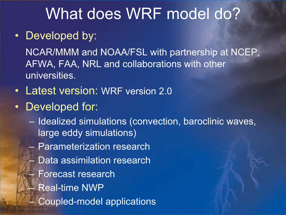
What does WRF model do?• Developed by:
NCAR/MMM and NOAA/FSL with partnership at NCEP, AFWA, FAA, NRL and collaborations with other universities.
• Latest version: WRF version 2.0
• Developed for:– Idealized simulations (convection, baroclinic waves,
large eddy simulations)– Parameterization research– Data assimilation research– Forecast research– Real-time NWP– Coupled-model applications


WRF Standard Initialization• Provides all required initial and time-varying
boundary conditions• De-grib GRIB files for meteorological data• Provides method to define and localize WRF
domain, nests, and subnests• Produces terrain, landuse, etc on domain:
– USGS 30 sec (~1km) topography– USGS 24 category landuse– WMO/FAO 16 category 2-layer soil types– Annual mean deep soil temperatures– Monthly greenness fraction– Albedo– Terrain slope index– Max Snow Albedo


WRF Dynamics
• Terrain Representation• Vertical Coordinate• Grid Staggering• Time integration scheme• Conservation Equations• Advection Scheme• Boundary conditions

Terrain Representation• Lower boundary
condition for geopotentialspecifies the terrain elevation
Vertical Coordinate
• Hydrostatic pressure• Vertical resolution set by user in WRFSI
(default: 31 levels)• Can choose option for vertical interpolation
(log, linear, square root)

Grid Staggering
Time-split Leap Frog and Runge-Kutta scheme
• 3rd order RK generally stable using timestep twice as large in leapfrog model
• Courant number limited to Cr = U∆t/ ∆x < 1.73
• C grid spacing

• RK3 method excellent scheme for integrating the compressible equations and is ideal candidate for NWP
• RK3 best combination of accuracy and simplicity
Wicker and Skamarock, 2002 MWR

Phase and Amplitude errors for LF and RK3

Phase and Amplitude errors for LF and RK3

Conservation Equations Mass Coordinate (Flux)
Momentum
Heat
Continuity
DiagnosticRelations
Ideal Gas LawHydrostatic pressure

Conservation Equation Height Coordinates (Flux)
Momentum
Heat
Continuity
ConservativeVariables
Pressure terms related to Θ
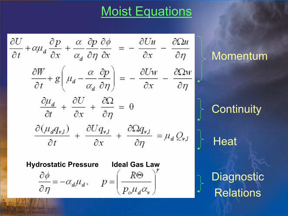
Moist Equations
Momentum
Continuity
Heat
DiagnosticRelations
Hydrostatic Pressure Ideal Gas Law

Advection • 2nd, 3rd, 4th,
5th,and 6th
order centered and upwind biased schemes
For constant U

Boundary ConditionsTop
1. Constant pressure2. Absorbing upper layer (increased horizontal diffusion)
Bottom1. Free Slip 2. Variety BL implementations on surface drag and fluxes
Lateral1. Specified 2. Open (perturbations can pass into/out of model domain)3. Symmetric4. Periodic (values of dependent variables are assumed
identically equal to values of another boundary)5. Nested
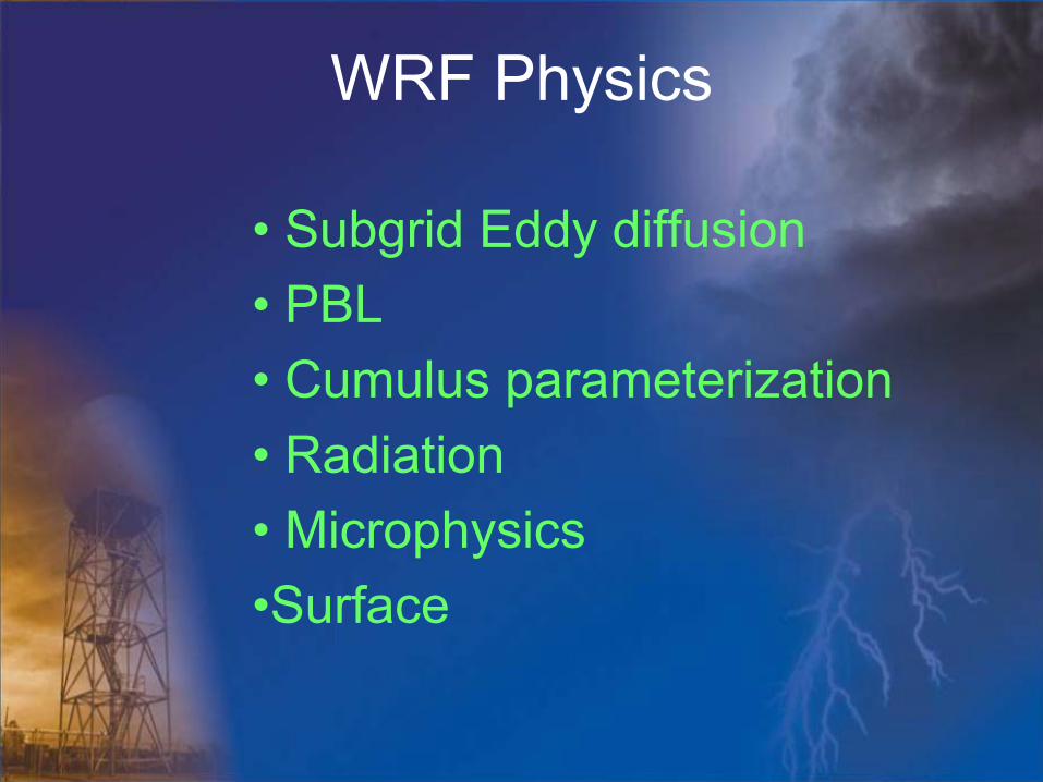
WRF Physics
• Subgrid Eddy diffusion• PBL• Cumulus parameterization• Radiation• Microphysics•Surface

Parameterizations Interactions

• It appears that the physic options are done within each RK loop EXCEPT the microphysics
• Microphysics:– Heat/moisture
tendencies– Microphysics
rates– Surface
rainfall
Parameterizations Interactions
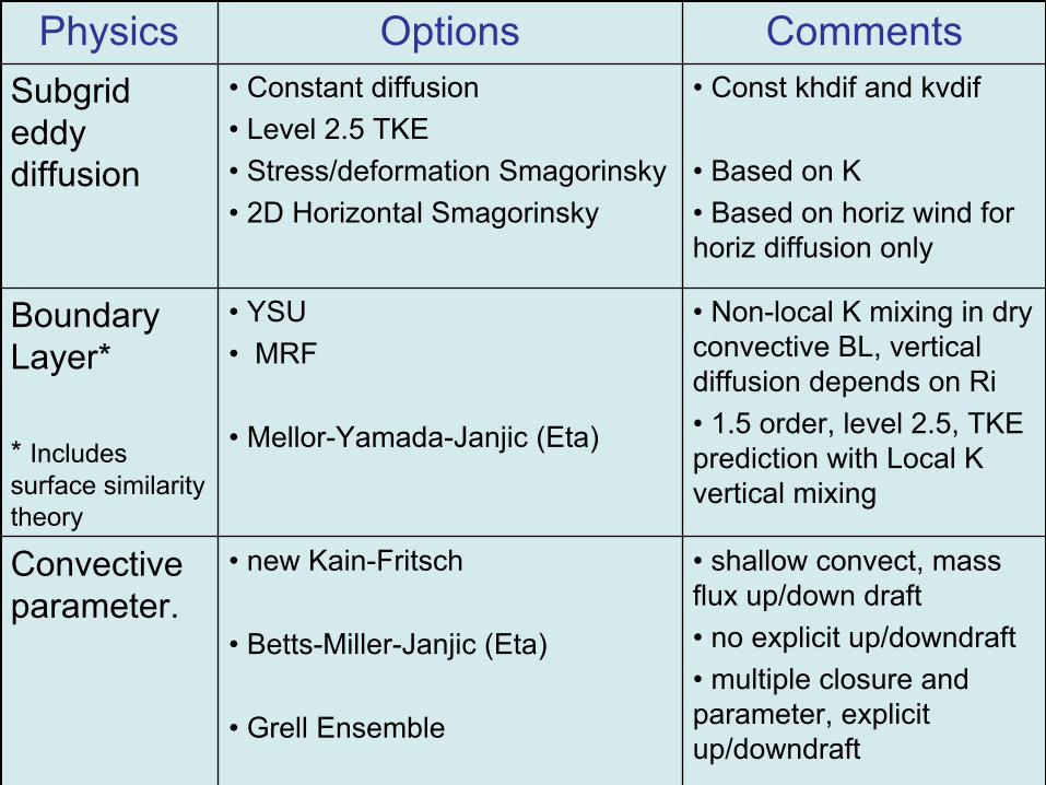
• shallow convect, mass flux up/down draft• no explicit up/downdraft• multiple closure and parameter, explicit up/downdraft
• new Kain-Fritsch
• Betts-Miller-Janjic (Eta)
• Grell Ensemble
Convective parameter.
• Non-local K mixing in dry convective BL, vertical diffusion depends on Ri• 1.5 order, level 2.5, TKE prediction with Local K vertical mixing
• YSU• MRF
• Mellor-Yamada-Janjic (Eta)
Boundary Layer*
* Includes surface similarity theory
• Const khdif and kvdif
• Based on K• Based on horiz wind for horiz diffusion only
• Constant diffusion• Level 2.5 TKE• Stress/deformation Smagorinsky• 2D Horizontal Smagorinsky
Subgrideddy diffusion
CommentsOptionsPhysics

• layers 1,2,4,8,and 16 cm thick• soil temp and moisture 4 layers• soil temp and moisture 6 layers
• 5 layer thermal diffusion • NOAH Land Surface• RUC Land Surface
Land-Surface
• warm rain, no ice, idealized • 5 class including graupel• 3 class with ice, ice processes• 5 class with ice, supercooled H20• one prognostic total condensate• 6 class with graupel
• Kessler• Lin et al.• WSM3• WSM5• Eta (Ferrier)• WSM6
Micro-physics
• Simple downward calculation, clear scattering•Spectral method• Used in Eta, ozone effects and interacts with clouds
• Dudhia (MM5)
• Goddard
• Eta (GFDL)
ShortwaveRadiation
• Spectral scheme with K distribution and a look up table• Spectral scheme from global model used in Eta
• RRTM (MM5)
• Eta (GFDL)
LongwaveRadiation
CommentsOptionsPhysics

Testing and Verification• Simulations
run to target specific facets of research or forecasting.
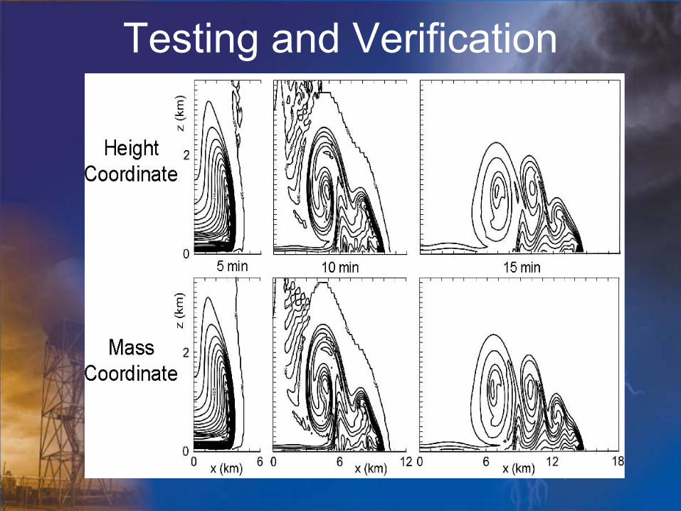
Testing and Verification

Testing and Verification

VerificationWeisman et al.– Although the 4 km
is typically minimum grid resolution, there was significant improvement in representing the system scale structure for larger convective systems
– Isolated convective outbreaks were not as well represented
– During International H20 project (IHOP)

VerificationBaldwind and
Wandishin– Found that WRF
reproduced the observed spectra much better than higher resolution Eta
– 10 km WRF model forecast maintains the variance in precip field down to at least 4 times grid spacing (40km)
– Variance of Eta drops off sooner and at greater than 10 times grid spacing
3 hr accumulated precipitation valid at 18Z from 12Z 4 June 2002 model run.

Computational EfficiencyMichalakes et al.– WRF is more costly in
terms of time-per-time step
– BUT the RK3 allows for considerably longer time step (200sec WRF vs. 81sec MM5)
– Time-to-solution performance for WRF slightly better than MM5
– Authors feel this will improve with tuning and optimization 36km resolution on a 136 x112 x 33 grid

Summary of WRF
• Fully compressible, non-hydrostatic (with hydrostatic option)
• Eulerian mass/height based terrain following coordinate• Arakawa C staggering• Runge-Kutta time integration scheme• Higher order advections• Scalar-conserving• Complete Coriolis and curvature• Two-way and one-way nesting• Lateral boundary conditions for ideal or real data• Full physics options

Questions?
ATMO 595ENovember 18, 2004
Melissa Goering Glen Sampson

ReferencesMichalakes et al.: Development of a Next-Generation Regional Weather
Research and Forecast Modelhttp://www.mmm.ucar.edu/mm5/mpp/ecmwf01.htm
Shamarock et al., 2001: Prototypes for the WRF Modelhttp://www.mmm.ucar.edu/individual/skamarock/meso2001pp_wcs.pdf
Weisman et al. 2002, : Preliminary Results from 4km Explicit Convective Forecasts Using the WRF Model. (Preprint) AMS 19th Conf. on Weather Analysis and Forecasting and 15th Conf. on Numerical Weather Prediction. Aug. 12th.
Wicker L.J. and W. Shamarock, 2002: Time-Splitting Methods for Elastic Models Using Forward Time Schemes. Mon. Wea. Rev., Vol. 130, pg. 2088-2097.
WRF model Users Web site: http://www.wrf-model.org