wavelets on irregular point sets - caltech multi-res …multires.caltech.edu/pubs/royal.pdf · ·...

Wavelets on Irregular Point Sets

B Y INGRID DAUBECHIES† , IGOR GUSKOV† ,PETER SCHRODER‡ , AND WIM SWELDENS∗

†Program for Applied and Computational Mathematics, Princeton University.‡Department of Computer Science, California Institute of Technology.

∗Lucent Technologies, Bell Laboratories.

[email protected], [email protected],[email protected], [email protected]

In this article we review techniques for building and analyzing wavelets on irregularpoint sets in one and two dimensions. We discuss current results both on the practicaland theoretical side. In particular we focus on subdivision schemes and commutationrules. Several examples are included.

1. Introduction

Wavelets are a versatile tool for representing general functions and data sets, and theyenjoy widespread use in areas as diverse as signal processing, image compression, finiteelement methods, and statistical analysis (among many others). In essence we may thinkof wavelets asbuilding blockswith which to represent data and functions. The particularappeal of wavelets derives from their representational and computationalefficiency: mostdata sets exhibit correlation both in time (space) and frequency, as well as other typesof structure. These can be modeled with high accurary through sparse combinations ofwavelets. Wavelet representations can also be computedfast, because they can be builtusing multiresolution analysis and subdivision.

Traditionally, wavelet functionsψj,m are defined as translates and dilates of one par-ticular function, themotherwaveletψ. We refer to these asfirst generationwavelets.This paper is concerned with a more general setting in which wavelets need not—andin fact, cannot—be translates and dilates of one or a few templates. Generalizations ofthis type were calledsecond generationwavelets in [39]; they make it possible to reapthe benefit of wavelet algorithms in settings with irregularly spaced samples, or on 2-manifolds which cannot be globally parameterized to the plane. In generalizing waveletanalysis to these more general settings one would like to preserve many of the proper-ties enjoyed by first generation wavelets. In particular, they should still be associatedwith fast algorithms and have appropriate smoothness and localization properties. In ad-dition, they should be able to characterize various functional spaces of interest. In thispaper we shall be mostly concerned with fast algorithms, localization, and smoothness;we will not address function space characterizations. Note though that the smoothnessof the wavelets is related to their ability to form unconditional bases for certain functionspaces [8][17].

Phil. Trans. R. Soc. Lond. A (1999) (Submitted) 1999 Royal Society Typescript

Printed in Great Britain 1 TEX Paper

2 I. Daubechies, I. Guskov, P. Schroder, W. Sweldens

The key to generalizing wavelet constructions to these non-traditional settings is theuse of generalizedsubdivision schemes. The first generation setting is already connectedwith subdivision schemes, but they become even more important in the constructionof second generation wavelets. Subdivision schemes provide fast algorithms, create anatural multiresolution structure, and yield the underlying scaling functions and waveletswe seek.

Subdivision is a technique originally intended for building smooth functions startingfrom a coarse description. In this setting there is no need for irregular grids, as one isfree to choose the finer grid to be regular. However, we intend to use subdivision as partof an entire multiresolution analysis which starts from a finest, irregular grid. This finestgrid is gradually “coarsified”; subdivision then gives an approximation of the originaldata by extrapolating the reduced data on the coarser grid back to the original finest grid.In such a setting the geometry of the grids is fixed by the finest irregular grid and thecoarsification procedure; thus subdivision on irregular grids is called for.Note: Another approach would be to resample the original finest level data on a regulargrid and use first generation wavelets. Resampling however can be costly, introduceartefacts, and is generally impossible in the surface setting. Therefore we choose to workon the original grid.

(a ) 1D SubdivisionThe main idea behind subdivision is the iteration of upsampling and local averaging to

build functions and intricate geometrical shapes. Originally such schemes were studiedin computer aided geometric design in the context of corner cutting [14][7] and the con-struction of piecewise polynomial curves, e.g., the de Casteljau algorithm for Bernstein-Bezier curves [13], and algorithms for the iterative generation of splines [31][1]. Latersubdivision was studied independently of spline functions [21][19][15][4][5][6] and theconnection to wavelets was made [33][9].

For example, Figure 1 demonstrates the application of the four point scheme. Newpoints are defined as local averages of two old points to the left and two old points to theright with weights(−1, 9, 9,−1)/16.

Figure 1. Subdivision is used to generate a smooth curve starting from a coarse description.

In the case of spline functions, smoothness follows from simple algebraic conditionson the polynomial segments at the knots. However, in the general setting convergenceand smoothness of the limit function are harder to prove. Various approaches have beenexplored to find the H¨older exponent of the limit function, or to determine its Sobolevclass. Early references in this context are [19][21][15][34][12][23][4] [36][41][24]. Thesestudies and their results all rely on regular, i.e., equi-spaced grids. The analysis uses toolssuch as the Fourier transform, spectral analysis, and the commutation formula.

In this paper we focus on irregular point sets. To describe the settings we are interestedin, we distinguish three types of refinement grids: regular, semi-regular, and irregular; seeFigure 2. Aregular grid has equidistant points on each level and each time a new pointis inserted exactly between two old points. For example, the curve shown in Figure 1 is

Phil. Trans. R. Soc. Lond. A (1999)

Wavelets on Irregular Point Sets 3

parameterized over a regular grid. Asemi-regulargrid (middle in Figure 2) starts withan irregular coarse grid and adds new points at parameter locations midway betweensuccessive old points. Thus the finer grids are locally regular except around the originalcoarsest level points. Inirregular grids (right) parameter locations of new points neednot be midway between successive old points. Note that regular grids are translation anddilation invariant, semi-regular grids are locally dilation invariant around coarsest levelvertices, and irregular grids generally possess no invariance property.

Similarly the weights used in subdivision schemes come in three categories: uniform,semi-uniform, and non-uniform.Uniformschemes like the four point scheme of Figure 1correspond to first generation wavelets; and use the same subdivision weights within alevel and across all levels; they are typically used on regular grids or grids which can besmoothly remapped to a regular grid.Semi-uniformschemes are used on semi-regulargrids; they vary the weights within each level (special weights are used in the neigh-borhood of the coarsest level points), but the same weights are used across levels. Suchschemes are sometimes referred to asstationary. Wavelets and subdivision schemes onan interval also fall in this category.Non-uniformschemes use varying weights withinandacross levels and correspond to the second generation setting.

Figure 2. Regular, semi-regular, and irregular grid hierarchies in 1D.

Almost all work on smoothness for non regular grids concerns the semi-regular gridswith semi-uniform subdivision schemes. Because translation-invariance is lost, Fouriertransform based arguments can no longer be used. However, since the same weightsare used on successive levels, one has dilation invariance around coarsest level pointsand can reduce the smoothness analysis to the study of spectral properties of certainfixed matrices. In [42][43] Warren shows that the semi-uniform version of the four pointscheme on a semi-regular grid yields aC1 limit function.

In the irregular case the subdivision scheme must become non-uniform to accountfor the irregularity of the associated parameter locations. This is illustrated in Figure 3which shows the limit functions of the uniform four point rule (left) and non-uniformfour point rule [40] (right); both use the same irregular grid.

Figure 3. An example why non-uniform subdivision is needed. Left the limit function with uniformsubdivision, right non-uniform. The same irregular grid is used in both figures.

The study of irregular subdivision is not only theoretically interesting, but also of greatimportance in practical applications. For example, in the semi-regular setting, one canuse adapted weights to better control the shape of a curve [30] or surface [45]. Moreimportantly, in many practical setups we start with samples associated to a very fine, butirregular grid. Now the main task for subdivision is not further refinement but rather aidin a multiresolution analysis oncoarsergrids. The wavelet and scaling functions fromthe coarsest level are generated with a subdivision scheme with new points which are no



longer parametric midpoints, but are dictated by the finest level grid on which the datawas originally sampled. Even though the actual number of levels is always finite for anyconcrete application of these methods, the asymptotic behavior of irregular subdivisionis still relevant as the finest and coarsest level could be arbitrarily far apart.

In these settings smoothness results become much harder to obtain. Because the sub-division weights vary within a level, the Fourier transform can no longer be used, andbecause they vary across levels even spectral analysis cannot help. In this paper we dis-cuss some tools that can be used to analyze smoothness; in particular we demonstratethat the commutation formula still holds and becomes a critical tool for smoothnessanalysis.

Figure 4. 2D Loop Subdivision is used to generate a smooth surfaces from a coarse description.

(b ) 2D SubdivisionThe 2D setting appears in the context of generating smooth surfaces, see Figure 4.

Here regular grids are too restrictive. For example, tensor product settings are only ap-plicable for surfaces homeomorphic to a plane, cylinder, or torus due to the Euler char-acteristic. Historically this challenge was addressed by generalizing traditional splinepatch methods to the semi-regular setting [18] (bi-quadratic) [3] (bi-cubic) [32] (quarticbox-spline). Similar to the 1D setting researchers also developed interpolating construc-tions [22][45][28]. All these settings (and others since; for an overview see [37]) proceedby applying quadrisection to an initial mesh consisting of either quadrilaterals or trian-gles and thus belong to the semi-regular setting. The weights used in the subdivisionscheme are semi-uniform since they take into account the local neighborhood structureof a vertex, i.e., how many edge neighbors a given vertex has. As in the 1D semi-regularsetting spectral analysis is the key to understanding the smoothness of these construc-tions. We refer to [35][42][44][38] for more details.

The irregular setting appears in 2D just as in the 1D case when some finest irregularlevel is presented on input and the main task is to build a multiresolution analysis oncoarserlevels. In this case however, we can no longer define downsampling as simplyretaining every other sample. This brings us to the realm of mesh simplification; wepostpone the discussion of mesh simplification and the construction of appropriate non-uniform subdivision operators to Section 3.

Figure 5. Sections of regular, semi-regular, and irregular triangle grids in 2D.



(c ) Overview

This paper summarizes results obtained in [11][10][25][26]. We start with the onedi-mensional results of [11][10]. We show that even simple subdivision rules, such as cubicLagrange interpolation, can lead to very intricate subdivision operators. To control theseoperators, we use commutation: because the subdivision scheme maps the space of cu-bic polynomial sequences to itself, we can define derived subdivision schemes for thedivided difference sequences. These simpler schemes can then be used to prove growthbounds on divided differences of some order, corresponding to smoothness results forthe limit function of the original scheme. The commutation formula enables us to controlsmoothness and is the key to the construction of wavelets associated with the subdivisionscheme.

In [25] inspiration from the 1D analysis is used to tackle the much more complex 2Dcase. Again, differences and divided differences are introduced, which can be computedfrom level to level with their own derived subdivision scheme. Control on the growth ofthese divided differences then leads to smoothness results. In practice, finding the rightAnsatz for irregular subdivision in the 2D setting is much harder than in the alreadydifficult 1D case. Finally, we show how irregular subdivision schemes can be used inmultiresolution pyramids for 2D meshes embedded inR3 and review several applica-tions from [26]. The “wavelets” associated with these schemes are overcomplete and arerelated to frames rather than bases.

2. The one dimensional case

(a ) Multilevel grids

Consider gridsXj , which are strictly increasing sequences of points{xj,k ∈ R | k ∈Z}, and which are consecutive binary refinements of the initial gridX0, i.e.,Xj ⊂ Xj+1

andxj+1,2k = xj,k for all j andk. Thus in every refinement step we insert one oddindexed pointxj+1,2k+1 between each adjacent pair of “even” pointsxj,k = xj+1,2k andxj,k+1 = xj+1,2k+2, as in Figure 2. We definedj,k := xj,k+1 − xj,k. We shall also usethe termgrid sizeon levelj, for the quantitydj := supk dj,k. As j → ∞ we want thegrids to become dense, “with no holes left”; this translates to the requirement that thedj

be summable.Notes:

(i) The above multilevel grids are calledtwo-nested. One can also consider moregeneral irregular grids such asq-nested grids where we insertq−1 new points in betweenold points or even non-nested but “threadable” grids. See [10] for more details on this.

(ii) In case the ratio between the lengths of any two neighboring intervals is globallybounded, we call the gridhomogeneous. An example of an irregular two-nested grid thatis not homogeneous is built byxj+1,2k+1 = βxj,k + (1 − β)xj,k+1 whereβ is a fixedparameter satisfying0 < β < 1. This is an example of adyadicallybalanced grid: theratio between the lengths of two “sibling” intervalsdj,2l anddj,2l+1 is bounded. Howeverthe ratio betweendj,−1 = βj anddj,0 = (1 − β)j is unbounded.

(b ) Subdivision schemes

Subdivision starts with a set of initial function valuesf0 = {f0,k} which live onthe coarsest gridX0. The subdivision schemeS is a sequence of linear operatorsSj ,j > 0, which iteratively compute valuesfj = {fj,k} on the finer grids via the formula



fj+1 = Sj fj, or

fj+1,l =∑

k

Sj,l,k fj,k.

We consider onlylocal schemes in the sense that the above summation has a globally

��

��

��

��

��

��

��

��

��

��

��

��

��

��

��

��

��

��

��

��

��

��

��

��

��

��

��

��

��

��

��

��

��

��

��

��

��

��

��

��

��

��

��

��

��

��

��

Figure 6. On the left an interpolating scheme is applied to function values; the new function values areshown as open circles. On the right arrows show the dependencies in the computation of those values; thevertical dashed arrows indicate that function values that were already assigned are kept unchanged in thesubdivision, because this is an interpolating scheme.

bounded number of terms centered aroundk = 2l. Subdivision gives us values definedon the grid pointsxj,k. By connecting these points we can define a piecewise linearfunction fj(x), see Figure 6. Our ambition is to synthesize a continuous limit functionϕ(x) as the pointwise limit forj → ∞ of fj(x). We are interested in the existence andsmoothness ofϕ(x).

The subdivision coefficientsSj,k,l will depend on the application one has in mind. Wepointed out in the introduction that one cannot simply stick with the coefficients fromthe regular case; typically the coefficients need to be spatially varying, and will be linkedto the spatial variation of the grid.

One such subdivision scheme which allows for a spatial interpretation is Lagrangianinterpolating subdivision [19][21][15][16]. Here the valuefj+1,2k+1 at a new point isfound by defining a polynomial which interpolates the points(xj,l, fj,l) for l in the neig-borhood ofk, and evaluating this polynomial atxj+1,2k+1; see Figure 7. In the reg-

P (x)

xj,k+1 xj,k+2

xj+1,2k+1

xj,kxj,k−1

fj+1,2k+1

Figure 7. Cubic Lagrangian interpolation: The valuefj+1,2k+1 at the odd gridpointxj+1,2k+1 is ob-tained by evaluating a cubic polynomialP (x) interpolating values at 4 neighboring even gridpointsxj+1,2k−2 = xj,k−1, . . . , xj+1,2k+4 = xj,k+2.

ular cubic case, this corresponds to the standard four point scheme, withSj,2k+1,k =



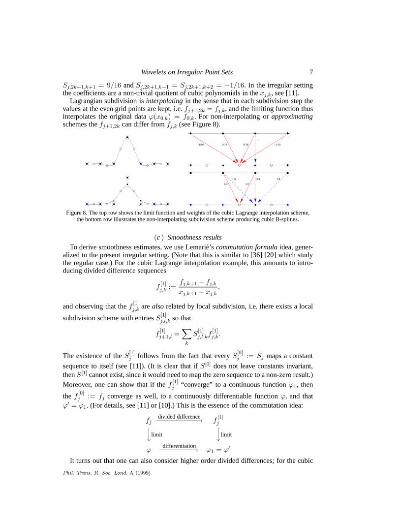
Sj,2k+1,k+1 = 9/16 andSj,2k+1,k−1 = Sj,2k+1,k+2 = −1/16. In the irregular settingthe coefficients are a non-trivial quotient of cubic polynomials in thexj,k, see [11].

Lagrangian subdivision isinterpolating in the sense that in each subdivision step thevalues at the even grid points are kept, i.e.fj+1,2k = fj,k, and the limiting function thusinterpolates the original dataϕ(x0,k) = f0,k. For non-interpolating orapproximatingschemes thefj+1,2k can differ fromfj,k (see Figure 8).

1

-1/169/169/16-1/16

��

��

��

��

��

��

��

��

��

��

��

��

��

��

��

��

��

��

��

��

1/83/4

1/2

1/8

1/2

��

��

��

��

Figure 8. The top row shows the limit function and weights of the cubic Lagrange interpolation scheme,the bottom row illustrates the non-interpolating subdivision scheme producing cubic B-splines.

(c ) Smoothness resultsTo derive smoothness estimates, we use Lemari´e’s commutation formulaidea, gener-

alized to the present irregular setting. (Note that this is similar to [36] [20] which studythe regular case.) For the cubic Lagrange interpolation example, this amounts to intro-ducing divided difference sequences

f[1]j,k :=

fj,k+1 − fj,k

xj,k+1 − xj,k,

and observing that thef [1]j,k arealso related by local subdivision, i.e. there exists a local

subdivision scheme with entriesS[1]j,l,k so that

f[1]j+1,l =

∑

k

S[1]j,l,kf

[1]j,k.

The existence of theS[1]j follows from the fact that everyS[0]

j := Sj maps a constant

sequence to itself (see [11]). (It is clear that ifS[0] does not leave constants invariant,thenS[1] cannot exist, since it would need to map the zero sequence to a non-zero result.)Moreover, one can show that if thef [1]

j “converge” to a continuous functionϕ1, then

the f [0]j := fj converge as well, to a continuously differentiable functionϕ, and that

ϕ′ = ϕ1. (For details, see [11] or [10].) This is the essence of the commutation idea:

fjdivided difference−−−−−−−−−−→ f

[1]jylimit

ylimit

ϕdifferentiation−−−−−−−−→ ϕ1 = ϕ′

It turns out that one can also consider higher order divided differences; for the cubic



Lagrange interpolation case, one can go up to fourth order differences becauseS[0]j maps

cubic polynomials sampled atxj,k to cubic polynomials sampled atxj+1,k. Thesef [4]j,k

no longer converge, but we can control their growth, and this helps us prove thatϕ1

is continuous, andϕ continuously differentiable. In fact, detailed (and rather technical)estimates in [11] show that, for homogeneous grids,

∣∣∣f [4]j,k

∣∣∣ 6 Cλj

d3j,k

,

whereλ < 1 is determined by the bound on the ratio between neighboring intervallengths. Once such a bound is known, a general theorem (see Theorem 4 in [11]) can beused to prove thatϕ ∈ C2−ε. This result is optimal in the sense that even in the regularcase, better smoothness cannot be obtained.Notes:

(i) This result for cubic Lagrange interpolation on homogeneous grids can be ex-tended to grids that are dyadically balanced only. The analysis becomes much moredelicate.

(ii) A similar approach can be used for non-interpolating subdivision. In that case itturns out that one has to use appropriately defined divided differences, which are differ-ent from the “standard” definition. See [10] for a complete discussion of this situation.

(d ) Wavelets

Wavelets at levelj are typically used, in the regular case, as the building blocks to rep-resent any function in the multiresolution analysis that “lives” in the(j + 1)-st approx-imation spaceVj+1, but not in the coarser resolution approximation spaceVj ⊂ Vj+1.One can introduce similar wavelets in the present irregular setting. The scaling func-tionsϕj,k are the limit functions obtained from starting the subdivision scheme at levelj, from the “initial” datafj,l = δl,k, and refining from there on. Under appropriate as-sumptions on the subdivision operatorsSj , theϕj,k are independent;Vj is the functionspace spanned by them. Clearly,Vj ⊂ Vj+1. As in the regular case, there are manydifferent reasonable choices for complement spacesWj (which will be spanned by thewavelets at levelj) that satisfyVj+1 = Vj ⊕Wj.

When the scaling functions are interpolating as in the Lagrangian case, i.e.,ϕj,k(xj,k′) =δk,k′ , then a simple choice for a wavelet is given byψj,m = ϕj+1,2m+1, i.e., the waveletis simply a finer scale scaling function at an odd location. This is sometime called aninterpolatingwavelet. This is in general not a very good wavelet as it does not have anyvanishing moments. It can be turned into a wavelet with vanishing moments using thelifting scheme [40].

Another way to select a complement spaceWj, is to use commutation between twobiorthogonal multiresolution hierarchies,Vj andVj. If both are associated to local sub-division schemes, then the biorthogonality of theϕj,k andϕj,l imposes consistency re-quirements on theSj andSj. Commutation can be used, as in the regular case, to passfrom one dual pair of multiresolution analyses to another, by operations related to differ-entiating and integrating, respectively. For instance, the above choice of an interpolatingwavelet corresponds formally to letting the dual scaling function be a Dirac. Applyingthe commutation rule each time reduces the order of the scaling functions, but increasesthe order of the dual scaling function. In particular the Dirac will become a box and lateron a general B-spline. It turns out that there is a natural definition of waveletsψj,k and



ψj,k corresponding to the dual multiresolution structures. It is shown in [10] that as inthe regular case the new wavelet after commutation is the derivative of the old waveletand the new dual wavelet is the integral of the old dual wavelet. By repeatedly applyingcommutation starting from the Lagrangian setting one can thus build the entire family ofbiorthogonal, compactly supported, irregular B-spline wavelets and their duals [10].

3. The two dimensional case

We mentioned in the introduction that the importance of the irregular setting arisesfrom the practical need to coarsify in settings in which the initial input is given as afunction over a fine triangulation of the plane (functional setting) or as a triangulation ofa 2-manifold (surface setting). In the 1D setting the downsampling operation to createa coarser level is straightforward as we can simply “skip” every other sample. In theirregular 2D setting downsampling is much less straightforward. Before delving intothe details of irregular 2D subdivision we first discuss a number of approaches whichcan be employed to define irregular downsampling in the surface setting. This problemhas received a lot of attention in computer graphics where it is generally referred to aspolygonal simplification.

(a ) Polygonal Simplification

In polygonal mesh simplification the goal is to simplify a given (triangulated) meshML = (PL,KL) into successively coarser, homeomorphic meshes(P l,Kl) with 0 6l < L, where(P0,K0) is the coarsest or base mesh. HereP l is a set ofl point positions,while Kl encodes the topological structure of the mesh and consists of triples{i, j, k}(triangles), pairs{i, j} (edges), and singletons{i} (vertices). The goal now is to allowcertain topological operations onKl which preserve the manifold property and genus ofthe mesh. These changes go hand in hand with geometric changes which are typicallysubject to an approximation quality criterion.

Several approaches for such mesh simplification have been proposed (the interestedreader is referred to the excellent survey [27] for more details). The most popular meth-ods are so called “progressive meshes” (PM). In a PM contruction a sequence of edgecollapses is prioritized based on the error it introduces. An edge collapse brings the end-points of the chosen edge into coincidence, in the process removing two triangles, threeedges, and one vertex (in the case of interior edges). The point location of the mergedvertex can be chosen so as to minimize some error criterion with respect to the originalmesh. The error can be measured in various norms such asL∞ (symmetric Haussdorffdistance),L2, and Sobolev norms.

For our purposes we are using a PM construction based on half edge collapses, i.e.,the point position for the collapsed edge is one of its end points. This results in a meshhierarchy which is interpolating in the sense that the point position setsP l are nested.There are several possible ways to define levels of a hierarchy. The most flexible onetreats a single half edge collapse operation as defining a level. In contrast to the usualwavelet setting this results in a linear, rather than logarithmic, number of levels.

Before going to the surface case we first consider the functional setting and then treatthe surface setting as three instances of a functional setting.



Figure 9. If an irregular, finely detailed mesh is given, the first task in building a multiresolution analysis iscoarsification.

(b ) Functional Setting: Multivariate commutation formula

Just as in the one dimensional case, irregular multivariate subdivision schemes act onsequences whose elements are associated with irregular parameter locations. We intro-duce levels numbered0, 1, . . . with level 0 corresponding to the coarsest scale. Withineach leveln the collection of all parameter locations constitute an irregular gridXn.

We can now introduce a subdivision schemeS as a sequence of linear operatorsSn,n > 0 which iteratively compute sequencesfn defined onXn, starting from some coars-est level dataf0, via

fn+1 = Snfn.

In the one-dimensional setting we analyzed the regularity of the functions produced bysubdivision through the behaviour of properly defined divided differences. We proceedsimilarly for the irregular two-dimensional setting. LetD[p]

n denote the operator whichmaps the data sequencefn into the corresponding sequencef [p]

n of divided differencesof orderp , that is,f [p]

n = D[p]n fn. We say that there exists a derived subdivision scheme

S[p] satisfying the commutation formula if the sequencesf[p]n are related via the relation

f[p]n+1 = S

[p]n f

[p]n where theS[p]

n constitute a local, bounded subdivision scheme. Thus we

can writeD[p]n+1Sn = S

[p]n D[p]

n . We then prove that the bounds on the growth of sequences

f[p]n can be translated into the smoothness estimates for the functions produced by the

original subdivision schemeS.In order to extend this construction to the multivariate case we need to define the mul-

tivariate divided differences in such a way that the algebra of the commutation formulaworks. This is done in [25] for a class of polynomial reproducing subdivision schemes.It is also shown there, that for multilevel grids satisfying some natural conditions, thebounds on the growth of these divided differences can be used to analyze the regularityof functions produced by subdivision.

(c ) Constructing a subdivision scheme

In this section we provide a particular example of a subdivision scheme which inthe functional setting produces visually smooth functions on irregular triangulations.Our subdivision algorithm relies on minimizing divided differences. Consider a triangle{i, j, k} in the parameter plane with corners(xi, yi), (xj , yj), and(xk, yk) and functionvaluesfi, fj, andfk. These three function values define a plane. The gradient to this



in 3D

difference of normals lies in parameter plane

2

k

j

1

function

values

plane is orthogonal

to 3D segment

angleright

l

l

and their difference;

triangle normals

common segment

parameter plane

plane contains both normals

Figure 10. Second differences are associated with an edge. Since they are the difference of two adjacenttriangle normals (first dividided differences) one can see that the second differences are orthogonal to thecommon edge in the parameter plane.

plane can be seen as a first order divided difference corresponding to this triangle. Thegradient is zero only if the plane is horizontal (fi = fj = fk).

Next we define the second order differences. They are computed as the differencebetween two normals on neighboring triangles and can be thought of as associated withthe common edge (see Figure 10, left). It is easy to see that the difference betweengradients of two adjacent triangles is orthogonal to their common edge (see Figure 10,right). Thus the componentD2

ef normal to the edgee can be used for the second orderdifference. It depends linearly on the four function values of these two triangles. Thecoefficients can be found in [25] or [26]. The second order difference operator is zeroonly if the two triangles lie in the same plane, and one can see that its behavior is closelyrelated to the dihedral angle.

The central ingredient in the design of our subdivision scheme is the use of a non-uniform relaxation operator which inserts new values in such a manner that second orderdifferences are minimized. Define a quadratic energy, which is an instance of a discretefairing functional [29]

Rfi = arg minE(fi) =∑

e∈K(D2

ef)2.

Setting∂E/∂fi = 0 yields

Rfi =∑

j∈V2(i)

wi,jfj with V2(i) = (3.1)

Note that iff is a linear function, i.e., all triangles lie in one plane, the fairing functionalE is zero. Consequently linear functions are invariant underR. In particularR preservesconstants from which we deduce that thewi,j sum to one.

Subdivision is computed one level at a time starting from leveln0 in the PM. Revers-ing the PM construction back to the finest level adds one vertex(xn, yn, fn) per level;the non-uniform subdivision is computed one vertex at a time. The position of each newvertexn is computed according to (3.1) using areas and lengths of the original finestlevel mesh. Next the immediate neighbors ofn are relaxed using (3.1) as well. The am-bition of our strategy of minimizingD2

ef is to obtainC1 smoothness. However, thereis currently no Ansatz on the bounds of the divided differences to prove regularity of



the limit function. Figure 11 shows an irregular grid of 20493 triangles (left), simplifieddown to 86 triangles (middle). Now associate the valuef = 1 with the center vertex and0 with all others. The figure on the right is the result of running the subdivision schemeback to the finest level. Even though the grid is irregular the resulting function appearssmooth.

Figure 11. From left to right: a portion of the fine mesh; the coarse mesh; function produced by thenon-interpolating scheme.

(d ) Functions on surfacesIn order to build a multiresolution structure on meshes we first need to introduce

the relaxation operator acting on functions defined over triangulated surfaces in 3D.We shall follow the strategy of the planar case and introduce second differences forsuch functions. For this we need to specify some locally consistent parameterizationover the support of the difference operator. Consider a triangular meshP in R3, andlet f : P → R. We would like to define the second difference operatorD2

ef for anedgee from the triangulationP. For this we only need a consistent parametrization (i.e.flattening) for two neighboring triangles at a time. Let the edgee = {i, j} be adjacentto two triangles{i, j, k} and{j, i, l}. We use the “hinge map” to build a pair of adjacenttriangles in the plane. These two triangles in the parameter plane have the same anglesand edge lengths as the two triangles inR3. We then defineD2

ef as described in theprevious section. Using these second differences, it is easy to extend the definition of therelaxation operator and the corresponding subdivision scheme to work with functionsdefined over triangulated surfaces.

(e) Burt-Adelson PyramidFor meshes we found it more useful to generalize an oversampled Burt-Adelson type

pyramid [2] than a critically sampled wavelet pyramid. Let(Pn) be some fixed PMhierarchy of triangulated surfaces. We start from the functionfN : P = PN → Rdefined on the finest level and compute a sequence of functions(fn) (n0 6 n 6 N ) as

well as oversampled differencesd(n)i between levels.

s(n-1)

(n)

Presmooth

d(n)s

Subdivision

Figure 12. Burt-Adelson style pyramid scheme.

Like subdivision, the Burt-Adelson pyramid is computed vertex by vertex. Thus thefour critical components of a BA pyramid: presmoothing, downsampling, subdivision,



and detail computation are done for one vertexn at a time (see Figure 12). The pres-moothing comes down to applying the relaxation operator to the neighbors ofn. Down-sampling simply removes the vertexn through a half edge collapse. We perform subdi-vision as described above and compute detailsd(n) for all neighbors ofn.

To see the potential of a mesh pyramid in applications it is important to understandthat the detailsd(n) can be seen as an approximate frequency spectrum of the mesh.The detailsd(n) with largen come from edge collapses on the finer levels and thuscorrespond to small scales and high frequencies, while the detailsd(n) with small ncome from edge collapses on the coarser levels and thus correspond to large scales andlow frequencies. Hence the sequence ofd(n) for runningn can be seen as an approximatefrequency spectrum. Moreover, while the superscriptn of an individual detail vectord(n)

icorresponds to its level/frequency, the subscripti corresponds to its location. Thus weactually have a space-frequency decomposition.

It is theoretically possible to build a critically sampled wavelet based on the Liftingscheme [39]. The idea is to use an interpolating subdivision scheme which only affectsthe new vertex and omits the relaxation of the even vertices. Consequently only one de-tail per vertex is computed and the sampling is always critical. However, at this pointit is not clear how to design updates that make the transform numerically stable. Addi-tionally, interpolating subdivision schemes do not yield very smooth meshes and haveunwanted undulations. Therefore critically sampled wavelet transforms have had limiteduse in graphics applications.

4. Applications

In the surface settingwe deal with a triangulated meshP of arbitrary topology andconnectivity embedded in 3D with verticespi = (xi, yi, zi). It is important to separatethe two capacities the meshP fulfills in our analysis. First, the original mesh and its PMrepresentation serve as the source of local parameterization and connectivity informationwhich determines the coefficients of our adaptive relaxation operator.

Second, if our purpose is to process the geometry of the mesh, it is crucial to treat allthree coordinatesx, y, andz asdependentvariables. In fact, we consider the coordinatesof the mesh to be real functions on the current PM vertex set. Initially, before any changesin geometry take place, these functions can be viewed as identities. When the wantedprocessing operations such as filtering or editing are applied to the data these functionsbecome more meaningful.

As an example of possible application of our scheme we present various manipula-tions of the scanned Venus’ head model. The original mesh has 50,000 vertices. Afterbuilding a PM hierarchy, we use our BA pyramid scheme to build a multiresolutionrepresentation. We can use different manipulations of the detail coefficients in order toachieve various signal processing tasks. Specifically, if all the detail coefficients finerthan some level are put to zero, we achieve a smoothing effect (in Figure 13(b) all thedetails on the levels above 1000 were set to zero). The stopband filter effect is achievedby setting to zero some range of coefficients (in Figure 13(c) all the details between thelevels 1000 and 15000 were set to zero). One can also enhance certain frequencies (inFigure 13(d) all the details between the levels 1000 and 15000 were multiplied by two).



Figure 13. Smoothing and filtering of the venus head. From left to right: (a) original; (b) low pass filter; (c)stopband filter; (d) enhancement filter.

5. Conclusion

One of the current frontiers in wavelet research and applications is the generalizationof multiresolution methods from the regular to the semi-regular and, more recently, ir-regular setting. We have given a brief review of these developments, starting with theone dimensional setting and moving on to the two dimensional functional and manifoldsettings. While there exists an extensive set of tools for the analysis of wavelet con-structions in the regular setting, such tools have only recently begun to emerge for theirregular setting. One such tool is the generalization of commutation from the regular tothe irregular setting. We have applied these ideas by proposing new irregular subdivisionschemes in the manifold setting which are explicitly designed to minimize certain dif-ferences. Little is as yet known about the analytic smoothness properties of the resultingconstructions, but numerical evidence suggests that they are quite useful for practicalapplications.

Acknowledgements

The work reviewed in this paper was supported in part by grants from NSF (ACI-9624957, ACI-9721349, DMS-9874082, DMS-9872890), DOE (W-7405-ENG-48), ONR(N00014-96-1-0367 P00004) and AFOSR (F49620-98-1-0044). Igor Guskov was par-tially supported by a Harold W. Dodds Fellowship and a Summer Internship at BellLaboratories, Lucent Technologies.

References[1] C. De Boor. A practical guide to splines. Number 27 in Applied Mathematical Sciences.

Springer, New York, 1978.

[2] P. J. Burt and E. H. Adelson. Laplacian pyramid as a compact image code. IEEE Trans.Commun., 31(4):532–540, 1983.

[3] E. Catmull and J. Clark. Recursively generated B-spline surfaces on arbitrary topologicalmeshes. Computer Aided Design, 10(6):350–355, 1978.

[4] A. S. Cavaretta, W. Dahmen, and C. A. Micchelli. Stationary subdivision. Memoirs Amer.Math. Soc., 93(453), 1991.



[5] A. S. Cavaretta and C. A. Micchelli. Computing surfaces invariant under subdivision. ComputerAided Geometric Design, 4(4):321–328, 1987.

[6] A. S. Cavaretta and C. A. Micchelli. The desing of curves and surfaces by subdivision algo-rithms. In T. Lyche and L. L. Schumaker, editors, Mathematical Aspects of Computer AidedGeometric Design. Academic Press, Tampa, 1989.

[7] G. Chaikin. An algorithm for high speed curve generation. Comp. Graphics Image Process.,3:346–349, 1974.

[8] W. Dahmen. Stability of multiscale transformations. J. Fourier Anal. Appl., 2(4):341–361,1996.

[9] I. Daubechies. Orthonormal bases of compactly supported wavelets. Comm. Pure Appl. Math.,41:909–996, 1988.

[10] I. Daubechies, I. Guskov, and W. Sweldens. Commutation for irregular subdivision. TechnicalReport, Bell Laboratories, Lucent Technologies, 1998.

[11] I. Daubechies, I. Guskov, and W. Sweldens. Regularity of irregular subdivision. Constr.Approx., 15:381-426, 1999.

[12] I. Daubechies and J. C. Lagarias. Two-scale difference equations I. Existence and globalregularity of solutions. SIAM J. Math. Anal., 22(5):1388–1410, 1991.

[13] F. de Casteljau. Outillages methodes calcul. Andre Citroen Automobiles SA, Paris, 1959.

[14] G. de Rham. Sur une courbe plane. J. Math. Pures Appl., 39:25–42, 1956.

[15] G. Deslauriers and S. Dubuc. Interpolation dyadique. In Fractals, dimensions non entieres etapplications, pages 44–55. Masson, Paris, 1987.

[16] G. Deslauriers and S. Dubuc. Symmetric iterative interpolation processes. Constr. Approx.,5(1):49–68, 1989.

[17] D. L. Donoho. Interpolating wavelet transforms. Preprint, Department of Statistics, StanfordUniversity, 1992.

[18] D. Doo and M. Sabin. Analysis of the behaviour of recursive division surfaces near extraordinarypoints. Computer Aided Design, 10(6):356–360, 1978.

[19] S. Dubuc. Interpolation through an iterative scheme. J. Math. Anal. Appl., 114:185–204, 1986.

[20] N. Dyn, J. Gregory, and D. Levin. Analysis of uniform binary subdivision schemes for curvedesign. Constr. Approx., 7:127–147, 1991.

[21] N. Dyn, D. Levin, and J. Gregory. A 4-point interpolatory subdivision scheme for curve design.Comput. Aided Geom. Des., 4:257–268, 1987.

[22] N. Dyn, D. Levin, and J. A. Gregory. A butterfly subdivision scheme for surface interpolationwith tension control. ACM Trans. on Graphics, 9(2):160–169, April 1990.

[23] N. Dyn, D. Levin, and C. A. Micchelli. Using parameters to increase smoothness of curves andsurfaces generated by subdivision. Comput. Aided Geom. Des., 7:129–140, 1990.

[24] T. Eirola. Sobolev characterization of solutions of dilation equations. SIAM J. Math. Anal.,23(4):1015–1030, 1992.

[25] I. Guskov. Multivariate subdivision schemes and divided differences. Technical report, De-partment of Mathematics, Princeton University, 1998.

[26] I. Guskov, W. Sweldens, and P. Schroder. Multiresolution signal processing for meshes. InComputer Graphics Proceedings (SIGGRAPH ’99), pages 325-334, 1999.

[27] P. S. Heckbert and M. Garland. Survey of polygonal surface simplification algorithms. Technicalreport, Carnegie Mellon University, 1997.

[28] L. Kobbelt. Interpolatory subdivision on open quadrilateral nets with arbitrary topology. InProceedings of Eurographics 96, Computer Graphics Forum, pages 409–420, 1996.

[29] L. Kobbelt. Discrete fairing. In Proceedings of the Seventh IMA Conference on the Mathematicsof Surfaces, pages 101–131, 1997.

[30] L. Kobbelt and P. Schroder. Constructing variationally optimal curves through subdivion.Technical Report CS-TR-97-05, Department of Computer Science, California Institute of Tech-nology, 1997.

[31] J. M. Lane and R. F. Riesenfeld. A theoretical development for the computer generation ofpiecewise polynomial surfaces. IEEE Trans. Patt. Anal. Mach. Intell., 3(1):35–46, 1980.



[32] C. Loop. Smooth subdivision surfaces based on triangles. Master’s thesis, University of Utah,Department of Mathematics, 1987.

[33] S. G. Mallat. Multiresolution approximations and wavelet orthonormal bases of L2(R). Trans.Amer. Math. Soc., 315(1):69–87, 1989.

[34] C. A. Micchelli and H. Prautzsch. Computing surfaces invariant under subdivision. ComputerAided Geometric Design, 4(4):321–328, 1987.

[35] U. Reif. A unified approach to subdivision algorithms near extraordinary vertices. ComputerAided Geometric Design, 12:153–174, 1995.

[36] O. Rioul. Simple regularity criteria for subdivision schemes. SIAM J. Math. Anal., 23(6):1544–1576, 1992.

[37] P. Schroder and D. Zorin, editors. Course Notes: Subdivision for Modeling and Animation.ACM SIGGRAPH, 1998.

[38] J. E. Schweitzer. Analysis and Application of Subdivision Surfaces. PhD thesis, University ofWashington, 1996.

[39] W. Sweldens. The lifting scheme: A construction of second generation wavelets. SIAM J.Math. Anal., 29(2):511–546, 1997.

[40] W. Sweldens and P. Schroder. Building your own wavelets at home. In Wavelets in ComputerGraphics, pages 15–87. ACM SIGGRAPH Course notes, 1996.

[41] L. F. Villemoes. Wavelet analysis of refinement equations. SIAM J. Math. Anal., 25(5):1433–1460, 1994.

[42] J. Warren. Subdivision methods for geometric design. Unpublished manuscript, Rice Universityhttp://www.cs.rice.edu/ ∼jwarren .

[43] J. Warren. Binary subdivision schemes for functions over irregular knot sequences. InM. Daehlen, T. Lyche, and L. Schumaker, editors, Mathematical Methods in CAGD III.Academic Press, 1995.

[44] D. Zorin. Ck continuity of subdivision surfaces. Technical report, California Institute ofTechnology, 1996.

[45] D. Zorin, P.Schroder, and W. Sweldens. Interpolating subdivision for meshes with arbitrarytopology. In Computer Graphics Proceedings (SIGGRAPH ’96), pages 189–192, 1996.


wavelets on irregular point sets - caltech multi-res …multires.caltech.edu/pubs/royal.pdf · ·...

Documents